Sin3DM: Learning a Diffusion Model from a Single 3D Textured Shape

Abstract.

Synthesizing novel 3D models that resemble the input example has long been pursued by researchers and artists in computer graphics. In this paper, we present Sin3DM, a diffusion model that learns the internal patch distribution from a single 3D textured shape and generates high-quality variations with fine geometry and texture details. Training a diffusion model directly in 3D would induce large memory and computational cost. Therefore, we first compress the input into a lower-dimensional latent space and then train a diffusion model on it. Specifically, we encode the input 3D textured shape into triplane feature maps that represent the signed distance and texture fields of the input. The denoising network of our diffusion model has a limited receptive field to avoid overfitting, and uses triplane-aware 2D convolution blocks to improve the result quality. Aside from randomly generating new samples, our model also facilitates applications such as retargeting, outpainting and local editing. Through extensive qualitative and quantitative evaluation, we show that our model can generate 3D shapes of various types with better quality than prior methods.

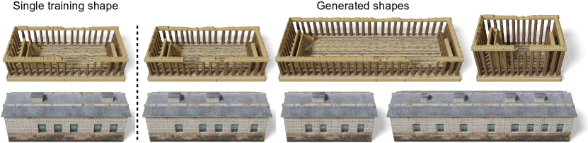
Figure 1. Trained on a single 3D textured shape (left), Sin3DM is able to produce a diverse new samples, possibly of different sizes and aspect ratios. The generated shapes depict rich local variations with fine geometry and texture details, while retaining the global structure of the training example. Top: acropolis (choly kurd, 2021); bottom: industry house (Lukas carnota, 2015).

1. Introduction

Creating novel 3D digital assets is challenging. It requires both technical skills and artistic sensibilities, often time-consuming and tedious. This motivates researchers to develop computer algorithms capable of generating new, diverse, and high-quality 3D models automatically. Over the past few years, deep generative models have demonstrated great promise for automatic 3D content creation (Achlioptas et al., 2018; Nash et al., 2020; Gao et al., 2022). More recently, diffusion models have proved particularly efficient for image generation and further pushed the frontier of 3D generation (Gupta et al., 2023; Wang et al., 2022c).

These generative models are typically trained on large datasets. However, collecting a large and diverse set of high-quality 3D data, with fine geometry and texture, is significantly more challenging than collecting 2D images. Today, publicly accessible 3D datasets (Chang et al., 2015; Deitke et al., 2022) remain orders of magnitude smaller than popular image datasets (Schuhmann et al., 2022), insufficient to train production-quality 3D generative models. In addition, many artistically designed 3D models possess unique structures and textures, which often have no more than one instance to learn from. In such cases, conventional data-driven techniques may fall short.

In this work, we present Sin3DM, a diffusion model that only trains on a single 3D textured shape. Once trained, our model is able to synthesize new, diverse and high-quality samples that locally resemble the training example. Our generated samples come with 3D meshes and UV-mapped textures (or even textures that describe physics-based rendering materials), which can be used directly in modern graphics engine such as Blender (Community, 2018) and Unreal Engine (Epic Games, 2019). We show example results in Fig. 1 and include more in Sec. 4. Our model also facilitates applications such as retargeting, outpainting and local editing.

We aim to train a diffusion model on a single 3D textured shape with locally similar patterns. Two key technical considerations must be taken into account. First, we need an expressive and memory-efficient 3D representation. Training a diffusion model simply on 3D grids would induce large memory and computational cost. Second, the receptive field of the diffusion model needs to be small, analogously to the use of patch discriminators in GAN-based approaches (Shaham et al., 2019). A small receptive field forces the model to capture local patch features.

The training process of our Sin3DM consists of two stages. We first train an autoencoder to compress the input 3D textured shape into triplane feature maps (Peng et al., 2020), which are three axis-aligned 2D feature maps. Together with the decoder, they implicitly represent the signed distance and texture fields of the input. Then we train a diffusion model on the triplane feature maps to learn the distribution of the latent features. Our denoising network is a 2D U-Net with only one-level of depth, whose receptive field is approximately $40\%$ of the feature map size. Furthermore, we enhance the generation quality by incorporating triplane-aware 2D convolution blocks, which consider the relation between triplane feature maps. At inference time, we generate new 3D textured shapes by sampling triplane feature maps using the diffusion model and subsequently decoding them with the triplane decoder.

To our best knowledge, Sin3DM is the first diffusion model trained on a single 3D textured shape. We demonstrate generation results on various 3D models of different types. We also compare to prior methods and baselines through quantitative evaluations, and show that our proposed approach achieves better quality.

2. Related Work

3D shape generation

Since the pioneering work by (Funkhouser et al., 2004), data-driven methods for 3D shape generation has attracted immense research interest. Early works in this direction follow a synthesis-by-analysis approach (Merrell, 2007; Bokeloh et al., 2010; Kalogerakis et al., 2012; Xu et al., 2012). After the introduction of deep generative networks such as GAN (Goodfellow et al., 2014), researchers start to develop deep generative models for 3D shapes. Most of the existing works primarily focus on generating 3D geometry of various representations, including voxels (Wu et al., 2016; Chen et al., 2021), point clouds (Achlioptas et al., 2018; Yang et al., 2019; Cai et al., 2020; Li et al., 2021), meshes (Nash et al., 2020; Pavllo et al., 2021), implicit fields (Chen and Zhang, 2019; Park et al., 2019; Mescheder et al., 2019), structural primitives (Li et al., 2017; Mo et al., 2019; Jones et al., 2020), and parametric models (Chen et al., 2020; Wu et al., 2021; Jayaraman et al., 2022). Some recent works take a step forward to generate 3D textured shapes (Gupta et al., 2023; Gao et al., 2022; Nichol et al., 2022; Jun and Nichol, 2023). All these methods rely on a large 3D dataset for training. Yet, collecting a high-quality 3D dataset is much more expensive than images, and many artistically designed shapes have unique structures that are hard to learn from a limited collection. Without the need of a large dataset, from merely a single 3D textured shape, our method is able to learn and generate its high-quality variations.

Another line of recent works (Poole et al., 2022; Lin et al., 2023; Wang et al., 2022b; Metzer et al., 2022; Liu et al., 2023) use gradient-based optimization to produce individual 3D models by leveraging differentiable rendering techniques (Mildenhall et al., 2020; Laine et al., 2020) and pretrained text-to-image generation models (Rombach et al., 2022). However, these methods have a long inference time due to the required per-sample optimization, and the results often show high saturation artifact. They are unable to generate fine variations of an input 3D example.

Single instance generative models

The goal of single instance generative models is to learn the internal patch statistics from a single input instance and generate diverse new samples with similar local content. The seminal work SinGAN (Shaham et al., 2019) explores this problem by training a hierarchy of patch GANs (Goodfellow et al., 2014) on an image pyramid. Many follow-up works improve upon it from various perspectives (Hinz et al., 2021; Shocher et al., 2019; Granot et al., 2021; Zhang et al., 2021). Some recent works use a diffusion model for single image generation by limiting the receptive field of the denoising network (Nikankin et al., 2022; Wang et al., 2022a) or constructing a multi-scale diffusion process (Kulikov et al., 2022). Our method is inspired by the above generative models trained on single image.

The idea of single image generation has been extended to other data domains, such as videos (Haim et al., 2021; Nikankin et al., 2022), audio (Greshler et al., 2021), character motions (Li et al., 2022; Raab et al., 2023), 3D shapes (Hertz et al., 2020; Wu and Zheng, 2022) and radiance fields (Karnewar et al., 2022; Son et al., 2022; Li et al., 2023). In particular, SSG (Wu and Zheng, 2022) is the most relevant prior work. It uses a multi-scale GAN architecture and trains a voxel pyramid of the input 3D shape. However, it only generates un-textured meshes (i.e., the geometry only) and the geometry quality is limited by the highest training resolution of the voxel grids. By encoding the input 3D textured shape into a neural implicit representation, our method is able to generate textured meshes with high resolutions for both geometry and texture.

A concurrent work (Li et al., 2023) uses a patch matching approach to synthesize 3D scenes from a single example. It specifically focuses on 3D natural scenes represented as grid-based radiance fields called Plenoxels (Fridovich-Keil et al., 2022). Therefore, its generated results cannot be easily re-lighted or imported into the existing graphics pipeline (such as the Unreal Engine (Epic Games, 2019)). In comparison, our method generates 3D shapes with UV-mapped textures, which can be directly used in modern graphics engines. Furthermore, we also support physics-based rendering (PBR) materials that are now commonly used for 3D assets.

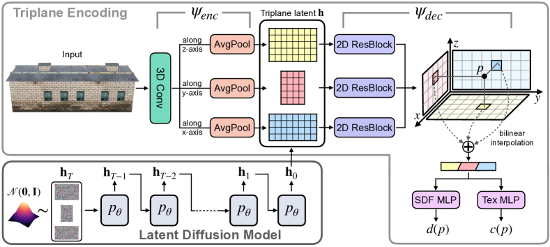
Figure 2. Method overview. Given an input 3D textured shape, we first train a triplane auto-encoder to compress it into an implicit triplane latent representation $\mathbf{h}$. Then we train a latent diffusion model on it to learn the distribution of triplane features. See Fig. 3 for the structure of our denoising network $p_{\theta}$. At inference time, we sample a new triplane latent using the diffusion model and then decode it to a new 3D textured shape using the triplane decoder $\psi_{\text{dec}}$.

Diffusion models

Diffusion models (Sohl-Dickstein et al., 2015; Ho et al., 2020; Song et al., 2020) are a class of generative models that use a stochastic diffusion process to generate samples matching the real data distribution. Recent works with diffusion models achieved state-of-the-art performance for image generation (Rombach et al., 2022; Dhariwal and Nichol, 2021; Saharia et al., 2022; Ramesh et al., 2022). Following the remarkable success in image domain, researchers start to extend diffusion models to 3D (Zeng et al., 2022; Nichol et al., 2022; Cheng et al., 2022; Shue et al., 2022; Gupta et al., 2023) and obtain better performance than prior GAN-based methods. These works typically train diffusion models on a large scale 3D shape dataset such as ShapeNet (Chang et al., 2015) and Objaverse (Deitke et al., 2022). In contrast, we explore the diffusion model trained on a single 3D textured shape to capture the patch-level variations.

3. Method

Overview

Sin3DM learns the internal patch distribution from a single textured 3D shape and generates high-quality variations. The core of our method is a denoising diffusion probabilistic model (DDPM) (Ho et al., 2020). The receptive field of the denoising network is designed to be small, analogously to the use of patch discriminators in GAN-based approaches (Shaham et al., 2019). With that, the trained diffusion model is able to produce patch-level variations while preserving the global structure (Wang et al., 2022a; Nikankin et al., 2022).

Directly training a diffusion model on a high resolution 3D volume is computationally demanding. To address this issue, we first compress the input textured 3D mesh into a compact latent space, and then apply diffusion model in this lower-dimensional space (see Fig. 2). Specifically, we encode the geometry and texture of the input mesh into an implicit triplane latent representation (Peng et al., 2020; Chan et al., 2021). Given the encoded triplane latent, we train a diffusion model on it with a denoising network composed of triplane-aware convolution blocks. After training, we can generate a new 3D textured mesh by decoding the triplane latent sampled from the diffusion model.

3.1. Triplane Latent Representation

To train a diffusion model on a high resolution textured 3D mesh, we need a 3D representation that is expressive, compact and memory efficient. With such consideration, we adopt the triplane representation (Peng et al., 2020; Chan et al., 2021) to model the geometry and texture of the input 3D mesh. Specifically, we train an auto-encoder to compress the input into a triplane representation.

Given a textured 3D mesh $\mathcal{M}$, we first construct a 3D grid of size $H\times W\times D$ to serve as the input to the encoder. At each grid point $p$, we compute its signed distance $d(p)$ to the mesh surface and truncate the value by a threshold $\epsilon_{d}$. For points whose absolute signed distance falls within this threshold, we set their texture color $c(p)\in\mathbb{R}^{3}$ to be the same as the color of the nearest point on the mesh surface. For points outside the distance threshold, we assign their color values to be zero. After such process, we get a 3D grid $G_{\mathcal{M}}\in\mathbb{R}^{H\times W\times D\times 4}$ of truncated signed distance and texture values. In our experiments, we set $\max(H,W,D)=256$.

Next, we use an encoder $\psi_{\text{enc}}$ to encode the 3D grid into a triplane latent representation $\mathbf{h}=\psi_{\text{enc}}(G_{\mathcal{M}})$, which consists of three axis-aligned 2D feature maps

(1) $$\mathbf{h}=(\mathbf{h}_{xy},\mathbf{h}_{xz},\mathbf{h}_{yz}),$$

where $\mathbf{h}_{xy}\in\mathbb{R}^{C\times H^{\prime}\times W^{\prime}}$, $\mathbf{h}_{xz}\in\mathbb{R}^{C\times H^{\prime}\times D^{\prime}}$ and $\mathbf{h}_{yz}\in\mathbb{R}^{C\times W^{\prime}\times D^{\prime}}$, with $C$ being the number of channels. $H^{\prime},W^{\prime},D^{\prime}$ are the spatial dimensions of the feature maps. The encoder $\psi_{\text{enc}}$ is composed of one 3D convolution layer and three average pooling layers for the three axes, as illustrated in Fig. 2.

The decoder $\psi_{\text{dec}}$ consists of three 2D ResNet blocks ($\psi_{\text{dec}}^{\text{xy}}$, $\psi_{\text{dec}}^{\text{xz}}$, $\psi_{\text{dec}}^{\text{yz}}$), and two separate MLP heads ($\psi_{\text{dec}}^{\text{geo}}$, $\psi_{\text{dec}}^{\text{tex}}$), for decoding the signed distances and texture colors, respectively. Consider a 3D position $p\in\mathbb{R}^{3}$. The decoder first refine the triplane latent $\mathbf{h}$ using 2D ResNet blocks and then gather the triplane features at three projected locations of $p$,

(2) $$\begin{split}f_{xy}&=\text{interp}(\psi_{\text{dec}}^{\text{xy}}(\mathbf{h}_{xy}),\;p_{xy}),\\ f_{xz}&=\text{interp}(\psi_{\text{dec}}^{\text{xz}}(\mathbf{h}_{xz}),\;p_{xz}),\\ f_{yz}&=\text{interp}(\psi_{\text{dec}}^{\text{yz}}(\mathbf{h}_{yz}),\;p_{yz}),\end{split}$$

where $\text{interp}(\cdot,q)$ performs bilinear interpolation of a 2D feature map at position $q$. The interpolated features are summed and fed into the MLP heads to predict the signed distance $\hat{d}$ and color $\hat{c}$,

(3) $$\begin{split}\hat{d}(p)&=\psi_{\text{dec}}^{\text{geo}}(f_{xy}+f_{xz}+f_{yz}),\\ \hat{c}(p)&=\psi_{\text{dec}}^{\text{tex}}(f_{xy}+f_{xz}+f_{yz}).\\ \end{split}$$

We train the auto-encoder using a reconstruction loss

(4) $$\mathcal{L}(\psi)={\mathbb{E}}_{p\in\mathcal{P}}[|\hat{d}(p)-d(p)|+|\hat{c}(p)-c(p)|],$$

where $\mathcal{P}$ is a point set that contains all the grid points and $5$ million points sampled near the mesh surface. $d(p)$ and $c(p)$ are the ground truth signed distance and color at position $p$, respectively.

We note that a seemingly simpler option is to follow an auto-decoder approach (Park et al., 2019), i.e., optimize the triplane latent $\mathbf{h}$ directly without an encoder. However, we found the resulting triplane latent $\mathbf{h}$ to be noisy and less structured, making the subsequent diffusion model hard to train. An encoder naturally regularizes the latent space. See Sec. 4.3 for an ablation study on this choice.

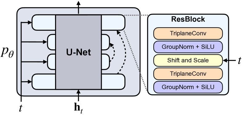
Figure 3. Denoising network structure. Our denoising network is a fully convolution U-Net composed of four ResBlocks and its bottleneck downsamples the input by $2$. Inside each ResBlock, we use the triplane-aware convolution layer (”TriplaneConv”), which is illustrated in Fig. 4.

3.2. Triplane Latent Diffusion Model

After compressing the input into a compact triplane latent representation, we train a denoising diffusion probabilistic model (DDPM) (Ho et al., 2020) to learn the distribution of these latent features.

At a high level, a diffusion model is trained to reverse a Markovian forward process. Given a triplane latent $\mathbf{h}_{0}=(\mathbf{h}_{xy},\mathbf{h}_{xz},\mathbf{h}_{yz})$, the forward process $q$ gradually adds Gaussian noise to the triplane features, according to a variance schedule $\{\beta_{t}\}_{t=0}^{T}$,

(5) $$q(\mathbf{h}_{t}\ |\mathbf{h}_{t-1})=\mathcal{N}(\mathbf{h}_{t}|\sqrt{1-\beta_{t}}\mathbf{h}_{t-1},\beta_{t}\mathbf{I}).$$

The noised data at step $t$ can be directly sampled in a closed form solution $\mathbf{h}_{t}=\sqrt{\bar{\alpha}_{t}}\mathbf{h}+\sqrt{1-\bar{\alpha_{t}}}\boldsymbol{\epsilon}$, where $\boldsymbol{\epsilon}$ is random noise drawn from $\mathcal{N}(\mathbf{0},\mathbf{I})$ and $\bar{\alpha}_{t}:=\prod_{s=1}^{t}\alpha_{s}=\prod_{s=1}^{t}(1-\beta_{s})$. With a large enough $T$, $\mathbf{h}_{T}$ is approximately random noise drawn from $\mathcal{N}(\mathbf{0},\mathbf{I})$.

A denoising network $p_{\theta}$ is trained to reverse the forward process. Due to the simplicity of the data distribution of a single example, instead of predicting the added noise $\boldsymbol{\epsilon}$, we choose to predict the clean input and thus train with the loss function

(6) $$\mathcal{L}(\theta)={\mathbb{E}}_{t\sim[1,T]}||\mathbf{h}_{0}-p_{\theta}(\mathbf{h}_{t},t)||_{2}^{2}.$$

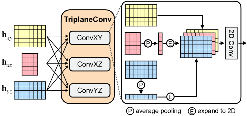
Figure 4. Triplane-aware convolution block. A TriplaneConv block considers the relation between triplane feature maps. Inside ConvXY, we apply axis-wise average pooling to $\mathbf{h}_{xz}$ and $\mathbf{h}_{yz}$, yielding two feature vectors, which are then expanded to the original 2D dimension by replicating along axis. The two expanded 2D feature maps are concatenated with $\mathbf{h}_{xy}$ and fed into a regular 2D convolution layer. ConvXZ and ConvYZ behaves similarly.

Denoising network structure.

A straight-forward option for the denoising network is to use the original U-Net structure from  (Ho et al., 2020), treating the triplane latent as images. However, this leads to ”overfitting”, namely the model can only generate the same triplane latent as the input $\mathbf{h}_{0}$, without any variations. In addition, it does not consider the relations between the three axis-aligned feature maps. Therefore, we design our denoising network to have a limited receptive field to avoid ”overfitting”, and use triplane-aware 2D convolution to enhance coherent triplane generation.

Figure 3 illustrates the architecture of our denoising network. It’s a fully-convolutional U-Net with only one-level of depth, whose receptive field covers roughly $40\%$ region of a triplane feature map of spatial size $128$. On the examples used in our experiments, we found that these parameter choices produce consistently plausible results and reasonable variations while keeping the input shape’s global structure. In each ResBlock in our U-Net, we use a triplane-aware convolution block (see  Fig. 4), similar to the one introduced in  (Wang et al., 2022c). It introduces cross-plane feature interaction by aggregating features via axis-aligned average pooling. As we will show in Sec. 4.3, it effectively improves the final generation quality.

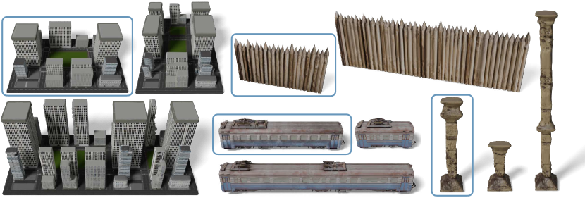
Figure 5. Retargeting results. By changing the spatial dimensions of the sampled Gaussian noise $\mathbf{h}_{T}$, we can resize the input to different sizes and aspect ratios. The training examples are labeled by blue boxes. From left to right, small town (Pedram Ashoori, 2020), wooden fence (REÂRCH Studio, 2018), train wagon (3ddominator, 2019) and antique pillar (oguzhnkr, 2017).

3.3. Generation

At inference time, we generate new 3D textured shape by first sampling new triplane latent using the diffusion model, and then decoding it using the triplane decoder $\psi_{\text{dec}}$. Starting from random Gaussian noise $\mathbf{h}_{T}\sim\mathcal{N}(\mathbf{0},\mathbf{I})$, we follow the iterative denoising process (Sohl-Dickstein et al., 2015; Ho et al., 2020),

(7) $$\mathbf{h}_{t-1}=\frac{\sqrt{\bar{\alpha}_{t-1}}\beta_{t}}{1-\bar{\alpha}_{t}}p_{\theta}(\mathbf{h}_{t},t)+\frac{\sqrt{\alpha_{t}}(1-\bar{\alpha}_{t-1})}{1-\bar{\alpha}_{t}}\mathbf{h}_{t}+\sigma_{t}\boldsymbol{\epsilon}$$

until $t=1$. Here, $\boldsymbol{\epsilon}\sim\mathcal{N}(\mathbf{0},\mathbf{I})$ for all but the last step ($\boldsymbol{\epsilon}=0$ when $t=1$) and $\sigma_{t}^{2}=\beta_{t}$. After obtaining the sampled triplane latent $\mathbf{h}_{0}$, we first decode a signed distance grid at resolution $256$, from which we extract the mesh using Marching Cubes (Lorensen and Cline, 1987). To get the 2D texture map, we use xatlas (Young, 2023) to warp the extracted 3D mesh onto a 2D plane and get the 2D texture coordinates for each mesh vertex. The 2D plane is then discritized into a $2024\times 2048$ image. For each pixel that is covered by a warped mesh triangle, we can obtain its corresponding 3D location via barycentric interpolation, and then query the decoder $\psi_{\text{dec}}^{\text{tex}}$ to obtain the RGB color at that pixel.

3.4. Implementation Details

For all examples tested in the paper, we use the same set of hyperparameters. The input 3D grid has a resolution $256$, i.e., $\max(H,W,D)=256$, and the signed distance threshold $\epsilon_{d}$ is set to $3/256$. The encoded triplane latent has a spatial resolution $128$, i.e., $\max(H^{\prime},W^{\prime},D^{\prime})=128$, and the number of channels $C=12$.

We train the triplane auto-encoder for $25000$ iterations using the AdamW optimizer (Loshchilov and Hutter, 2017) with an initial learning rate $5\mathrm{e}{-3}$ and a batch size of $2^{16}$. The triplane latent diffusion model has a max time step $T=1000$. We train it for $25000$ iterations using the AdamW optimizer with an initial learning rate $5\mathrm{e}{-3}$ and a batch size of $32$. With the above settings, the training usually takes $2\sim 3$ hours on an NVIDIA RTX A6000. Please see the supplementary document for detailed network configurations.

4. Experiments

4.1. Qualitative Results

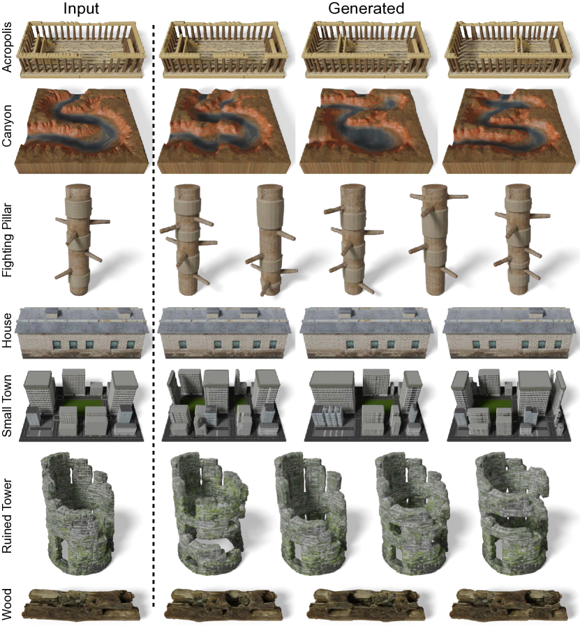
Figure 9. Results gallery. We show the input 3D textured shapes on the left, and several randomly generated samples on the right. From top to bottom, acropolis (choly kurd, 2021), canyon (Šimon Ustal, 2020), fighting pillar (ImpJive, 2021), house (Lukas carnota, 2015), small town (Pedram Ashoori, 2020), ruined tower (JB3D, 2019) and wood (All-about-Blender-3D, 2020). See Fig. 10 and the supplementary document for more examples.

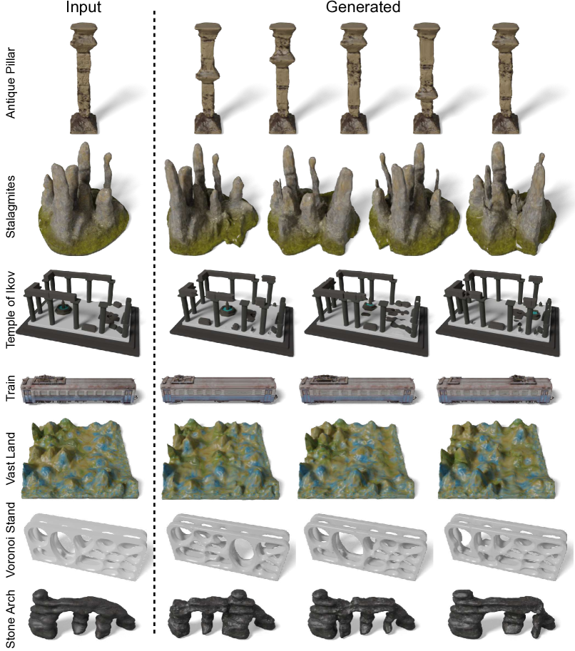
Figure 10. Results gallery. From top to bottom, antique pillar (oguzhnkr, 2017), stalagimites (Werniech van der Heever, 2019), temple of ikov (Laetitia Irata, 2019), train wagon (3ddominator, 2019), vast land (Shahriar Shahrabi, 2021), wooden fence (REÂRCH Studio, 2018), stone arch (Werniech, 2022).

We show a gallery of generated results in Fig. 9 and Fig. 10. By simply changing the spatial dimensions of the sampled Gaussian noise $\mathbf{h}_{T}$, we can resize the input to different sizes and aspect ratios while keeping the local content. We show those retargeting examples in Fig. 1 and Fig. 5. As can be seen, the generated shapes are able to preserve the global structure of the input example, while presenting reasonable local variations in terms of both geometry and texture. In the supplementary materials, we provide more visual results and also a webpage for interactive view of the generated 3D models.

Table 1. Quantitative comparison. $\downarrow$: lower is better; $\uparrow$: higher is better. We compare our method to SSG (Wu and Zheng, 2022) in terms of geometry quality (G-Qual.), geometry diversity (G-Div.), texture quality (T-Qual.) and texture diversity (T-Div.). The numbers for T-Qual. are multiplied by $1\times 10^{6}$. The last column is the average score over the 10 testing examples. Please refer to the supplementary document for the details regarding each evaluation metric.

Metrics	Methods	Examples
		Acropolis	Canyon	Cliff Stone	Fight Pillar	House	Stairs	Small Town	Tree	Wall	Wood	Avg.
G-Qual. $\downarrow$	Ours	0.059	0.075	0.075	0.181	0.069	0.283	0.600	0.064	0.113	0.043	0.156
	SSG	0.055	0.077	0.150	0.247	0.017	0.376	0.928	0.179	0.244	0.111	0.238
G-Div. $\uparrow$	Ours	0.139	0.166	0.285	0.169	0.010	0.204	0.528	0.518	0.078	0.140	0.224
	SSG	0.091	0.218	0.342	0.175	0.008	0.040	0.463	0.514	0.101	0.134	0.209
T-Qual. $\downarrow$	Ours	1.365	1.237	0.191	0.374	1.033	3.492	3.615	0.605	1.348	0.294	1.355
	SSG	2.933	3.234	0.770	3.265	1.913	5.316	19.362	13.239	2.869	0.287	5.319
T-Div. $\uparrow$	Ours	0.066	0.218	0.132	0.151	0.053	0.234	0.255	0.116	0.048	0.056	0.133
	SSG	0.066	0.267	0.187	0.194	0.079	0.181	0.250	0.132	0.080	0.063	0.150

4.2. Comparison

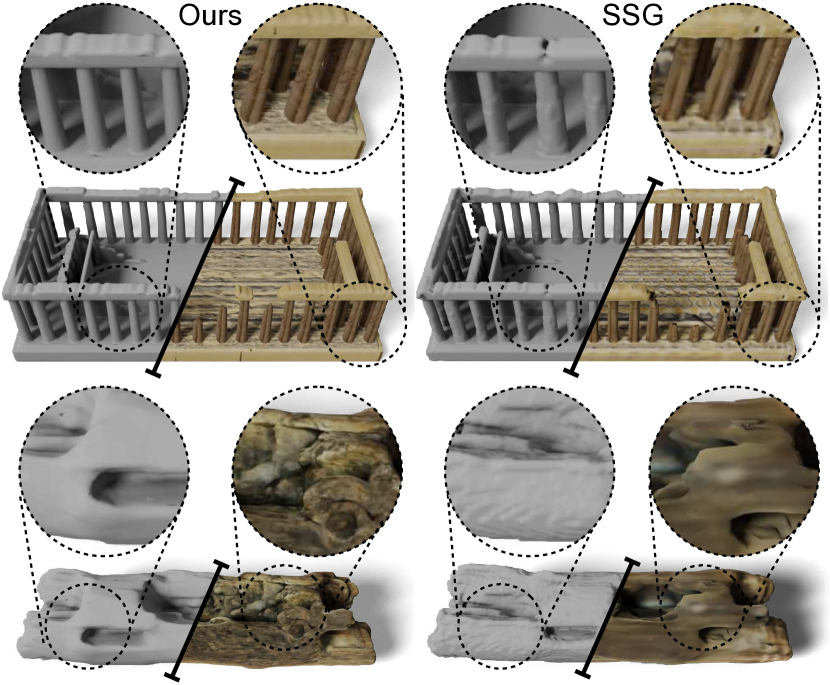
Figure 6. Visual comparison. We compare the generated results from our method (left) and SSG (right) (Wu and Zheng, 2022). The inputs of these two examples are shown in Fig. 9. Note that our mesh surfaces are much cleaner (see the zoomed-in columns), and our textures have much more details (see the zoomed-in wood surfaces).

We compare our method against SSG (Wu and Zheng, 2022), a GAN-based single 3D shape generative model. Since SSG only generates geometry, we extend it to support texture generation by adding 3 extra dimensions for RGB color at its generator’s output layer. For a fair comparison, we train it on the same sampled 3D grid (resolution $256$) that we used as our encoder input. In the supplementary document, we also include a comparison to the original SSG on geometry generation only, by removing the texture component (e.g., $\psi_{\text{dec}}^{\text{tex}}$) in our model.

Evaluation Metrics

To quantitatively evaluate the quality and diversity for both the geometry and texture of the generated 3D shapes, we adopt the following metrics. For geometry evaluation, we first voxelize the input shape and the generated shapes at resolution $128$. Geometry Quality (G-Qual.) is measured against the input 3D shape using SSFID (single shape Fréchet Inception Distance) (Wu and Zheng, 2022). Geometry Diversity (G-Div.) is measured by calculating the pair-wise IoU distance ($1-\text{IoU}$) among generated shapes.

For texture evaluation, we first render the input 3D model from $8$ views at resolution $512$. Each generated 3D model is then rendered from the same set of views. For the rendered images under each view, we compute the SIFID (Single Image Fréchet Inception Distance) (Shaham et al., 2019) against the image from the input model, and also compute the LPIPS metric (Zhang et al., 2018) between those images. Texture Quality (T-Qual.) is defined as the SIFID averaged over different views. Similarly, Texture Diversity (T-Div.) is defined as the LPIPS metric averaged over different views.

We select $10$ shapes in different categories as our testing examples. For each input example, we generate $50$ outputs to calculate the above metrics. More formal definition of the above evaluation metrics are included in the supplementary document.

Table 2. Ablation study. Metric values here are averages over the 10 testing examples used in Table 1. The numbers for T-Qual. are multiplied by $1\times 10^{6}$.

	G-Qual. $\downarrow$	G-Div. $\uparrow$	T-Qual. $\downarrow$	T-Div. $\uparrow$
Ours	0.156	0.224	1.355	0.133
w/o triplaneConv	0.347	0.310	3.453	0.171
w/o encoder	0.608	0.355	4.942	0.179
$\boldsymbol{\epsilon}$-prediction	0.925	0.402	4.401	0.187

Results

We report the quantitative evaluation results in Table 1, and highlight the visual difference in Fig. 6. Compared to SSG, our method obtains better scores for geometry and texture quality, while having similar scores for diversity. In particular, the mesh surfaces of our generated results are cleaner and smoother, and the textures contain much more details (see Fig. 6). This is largely due to the fact that SSG trains on voxelized representations. Therefore, the result quality is limited by the highest voxel resolution. In contrast, our method makes use of implicit signed distance and texture fields, which are able to represent much finer details.

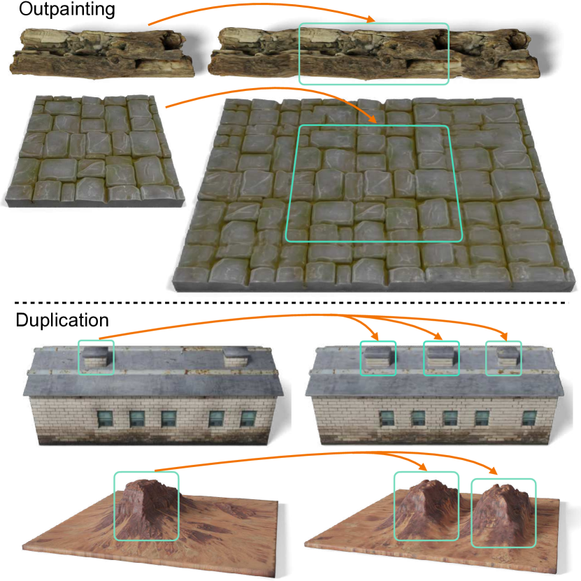
Figure 7. Controlled Generation. Top: outpainting, which seamlessly extend the input 3D shape beyond its boundaries. Bottom: patch duplication, which copies a patch of the input to specified locations of the generated outputs. Wood (All-about-Blender-3D, 2020), stone tiles (skinny hands, 2021), house (Lukas carnota, 2015) and sandstone mountain (Marti David Rial, 2021).

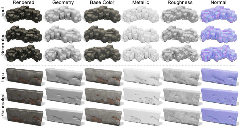
Figure 8. Results on 3D models with PBR material. Here we show two examples with PBR materials. For each example, we show the input model on top and two generated models below. Cliff stone (DJMaesen, 2021), damaged brick wall (Max Ramirez, 2016).

4.3. Ablation Study

We conduct ablation studies to validate several design choices of our method. Specifically, we compare our proposed method with the following variants:

Ours (w/o triplaneConv), in which we do not use the triplane-aware convolution (Fig. 4) in the denoising network. Instead, we simply use three separate 2D convolution layers for each plane, without considering the relation between triplane features.

Ours (w/o encoder), in which we remove the triplane encoder $\psi_{\text{enc}}$ and fit the triplane latent in an auto-decoder fashion (Park et al., 2019). The resulting triplane latent is less structured, making the subsequent diffusion model hard to train.

Ours ($\boldsymbol{\epsilon}$-prediction), in which the diffusion model predicts the added noise $\boldsymbol{\epsilon}$ instead of the clean input $\mathbf{h}_{0}$ (see Eqn. 6). In single example case, $\mathbf{h}_{0}$ is fixed and therefore easier to predict. Predicting the noise $\boldsymbol{\epsilon}$ adds extra burden to the diffusion model.

As shown in Table 2, all these variants lead to lower scores for geometry and texture quality. The diversity scores increase at the cost of much lower result quality. Please refer to the supplementary document for visual comparison.

4.4. Controlled Generation

Aside from randomly generating novel variations of the input 3D textured shape, we can also control the generation results by specifying a region of interest. Let $m$ denote a spatial binary mask indicating the region of interest. Our goal is to generate new samples such that the masked region $m$ stays as close as possible to our specified content $\mathbf{y}_{0}$ while the complementary region $(1-m)$ are synthesized from random noise. Specifically, when applying the iterative denoising process (Eqn. 7), we replace the masked region with $\mathbf{y}_{0}$. That is, $\mathbf{h}_{t-1}\odot m\leftarrow\mathbf{y}_{0}\odot m$, where $\odot$ is element-wise multiplication. To allow smooth transition around the boundaries, we adjust $m$ such that the borders between $0$ and $1$ are linearly interpolated. Note that no re-training is needed and all changes are made at inference time.

We demonstrate two use cases in Fig. 7. 1) Outpainting, which seamlessly extends the input 3D textured shape beyond its boundaries. This is achieved by setting $\mathbf{y}_{0}$ to be the padded triplane latent $\mathbf{h}_{0}$ of the input (padded by zeros). The mask $m$ corresponds to the region that is occupied by the input. 2) Patch duplication, which copies the a patch of the input to the certain locations of the generated outputs where other parts are synthesized coherently. In the case, we take $\mathbf{h}_{0}$ and copy the corresponding features to get $\mathbf{y}_{0}$. The mask $m$ corresponds to the regions where the copied patches reside.

4.5. Supporting PBR Material

PBR (Physics-Based Rendering) materials are commonly used in modern graphics engines, as they provide more realistic rendering results. Our method can be easily extended to support input 3D shape with PBR material. In particular, we consider the material in terms of base color ($\mathbb{R}^{3}$), metallic ($\mathbb{R}$), roughness ($\mathbb{R}$) and normal ($\mathbb{R}^{3}$). Then, the input 3D grid has $9$ channels in total (i.e., $G_{\mathcal{M}}\in\mathbb{R}^{H\times W\times D\times 9}$). We add two additional MLP heads in the decoder — one for predicting metallic and roughness; the other for predicting normal. We demonstrate some examples in Fig. 8, and provide more in the supplementary document.

5. Limitations and Future Work

In this work, we present Sin3DM, a diffusion model that is trained on a single 3D textured shape. To reduce the memory and computational cost, we compress the input into triplane feature maps and then train a diffusion model to learn the distribution of latent features. With a small receptive field and triplane-aware convolutions, our trained model is able to synthesize faithful variations with intricate geometry and texture details.

Our approach also has some limitations. Built upon diffusion models, our method inherits their limitation of relatively long inference time, due to the iterative nature of the sampling process. While the use of triplane representation significantly reduces the memory and computational cost, it introduces an implicit bias to our generative model. We empirically observed that the generated variations primarily occur along three axis directions. It’s an important future direction to develop a 3D representation that is expressive, efficient and also suitable for generative modeling.

Generative models that learn from a single instance well retain the local content of the training instance, but lack the ability to leverage prior knowledge from external datasets. Combing large pretrained generative models with single instance learning, possibly through fine-tuning (Ruiz et al., 2022; Zhang et al., 2022), is another interesting direction for synthesizing more diverse variations.

Appendix A Network Architectures

Table 3. Network architectures. IN: instance normalization layer. GN: group normalization layer. Downsampling: average pooling. Upsampling: bilinear interpolation with scaling factor 2. For the decoder MLP, we add a skip connection to the middle layer (Park et al., 2019).

Module	Layers	Out channels	Kernel size	Stride
$\psi_{\text{enc}}$ -conv	Conv3D+IN+tanh	12	4	2
$\psi_{\text{dec}}$ -ResBlock	Conv2D+IN+SiLU	64	5	1
	Conv2D	64	5	1
	Conv2D (shortcut)	64	1	1
$\psi_{\text{dec}}$ -MLP	5 [Linear+ReLU]	256	-	-
	Linear	1 or 3	-	-
$p_{\theta}$	TriplaneConv	64	1	1
	TriplaneResBlock	64	3	1
	Downsampling	-	2	2
	TriplaneResBlock	128	3	1
	TriplaneResBlock	128	3	1
	Upsampling	-	-	-
	TriplaneResBlock	64	3	1
	GN+SiLU+TriplaneConv	12	1	1

Appendix B Evaluation Metrics

For G-Qual. and G-Div., we refer readers to (Wu and Zheng, 2022) for the calculation of SSFID and diversity score based on IoU.

T-Qual. and T-Div. are computed as follows. We uniformly select 8 upper views (elevation angle $45^{\circ}$) and render the textured meshes in Blender. Let $I_{i}(M)$ and $I_{i}(G_{j})$ denote the rendered images at the $i-$th view, of the reference mesh $M$ and the generated mesh $G_{j}$, respectively. T-Qual. and T-Div. are then defined as

(8) $$\begin{split}\text{T-Qual.}&=\frac{1}{8}\sum_{i=1}^{8}[\frac{1}{n}\sum_{j=1}^{n}\text{SIFID}(I_{i}(M),I_{i}(G_{j}))],\\ \text{T-Div.}&=\frac{1}{8}\sum_{i=1}^{8}[\frac{1}{k(k-1)}\sum_{j=1}^{n}\sum_{\begin{subarray}{c}k=1\\ k\neq j\end{subarray}}^{n}\text{LPIPS}(I_{i}(G_{j}),I_{i}(G_{k}))],\end{split}$$

where we set $n=50$. SIFID(Shaham et al., 2019) and LPIPS (Zhang et al., 2018) are distance measures.

Appendix C More Results

Visual comparison for the ablation study is shown in Fig. 11 and Fig. 12. More generation results are shown in Fig. 13 and Fig. 14. We also compare to SSG (Wu and Zheng, 2022) on geometry generation only, by removing the texture component (e.g., $\psi_{\text{dec}}^{\text{tex}}$) in our model. In Table 4 and Fig. 15, we show the quantitative and qualitative evaluation results on their 10 testing examples.

Table 4. Quantitative comparison on geometry generation. $\downarrow$: lower is better; $\uparrow$: higher is better. Please refer to (Wu and Zheng, 2022) for metrics definition. Numbers are average values over 10 testing examples.

	LP-IoU $\uparrow$	LP-F-score $\uparrow$	SSFID $\downarrow$
Ours	0.572	0.699	0.068
SSG	0.477	0.594	0.074

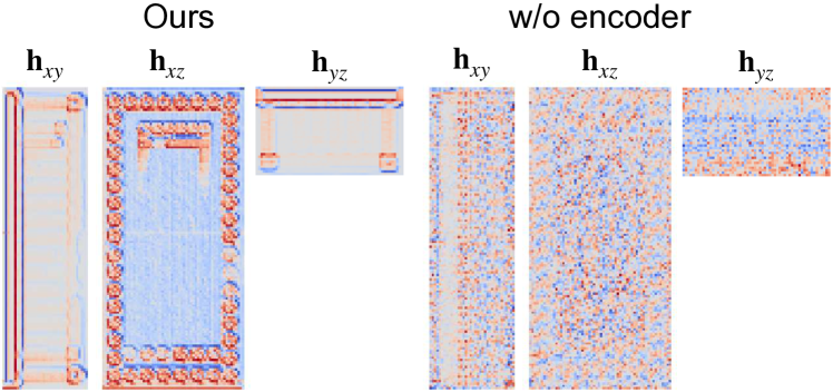
Figure 11. Ablation over triplane feature maps. Without an encoder, the learned triplane feature maps are noisy and less structured, which would pose a difficult task for the subsequent diffusion model.

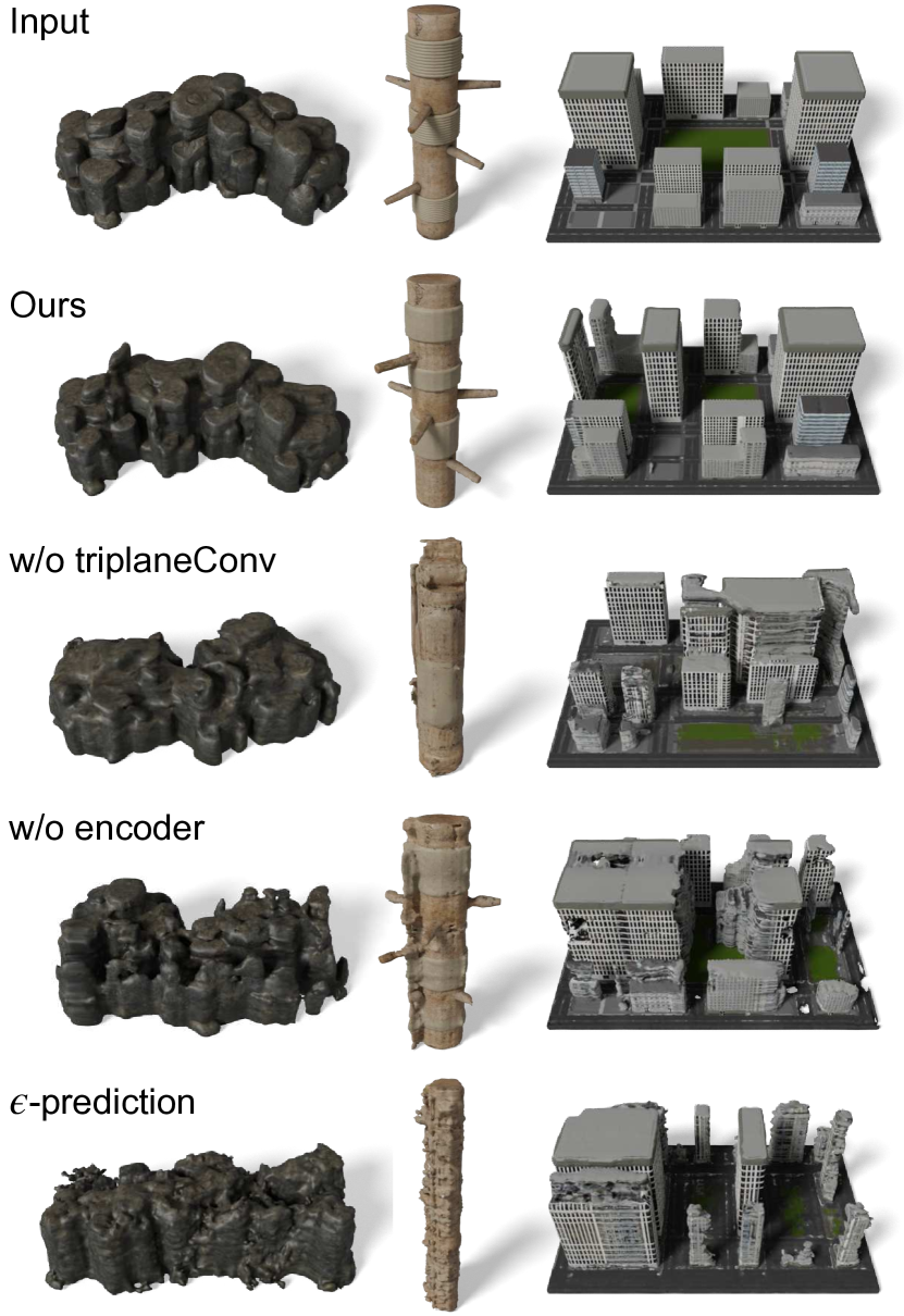
Figure 12. Ablation study. Here we show visual results from our proposed method and compared variants.

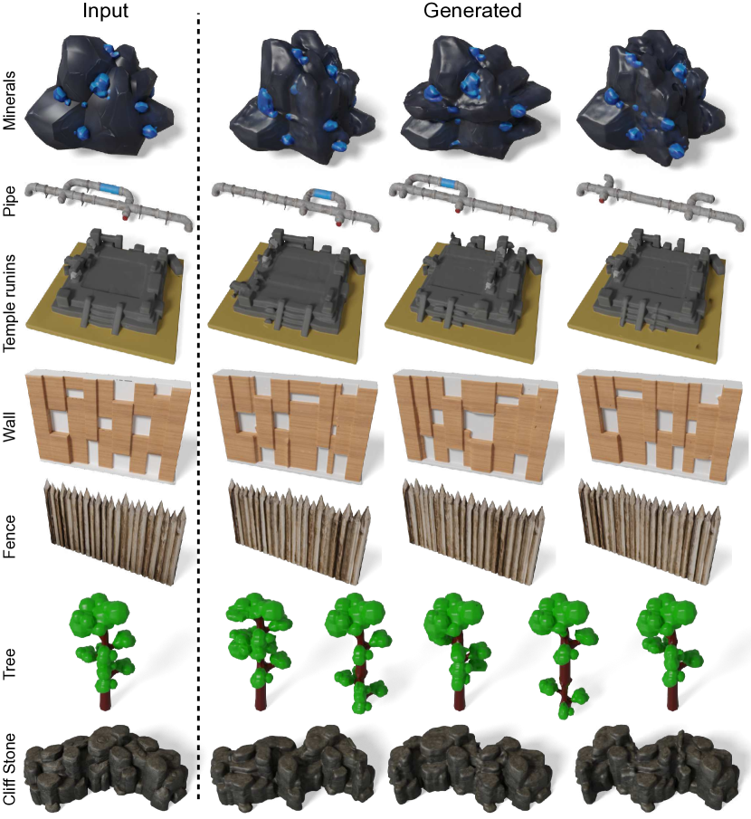
Figure 13. Results gallery. From top to bottom, minerals (Frybrix, 2018), pipe (SLASH / RENDAR, 2020), temple ruins (Deyama, 2018), wall (stray, 2015), voronoi (Ahmad Riazi, 2013), tree (nikola, 2020) and cliff stone (DJMaesen, 2021).

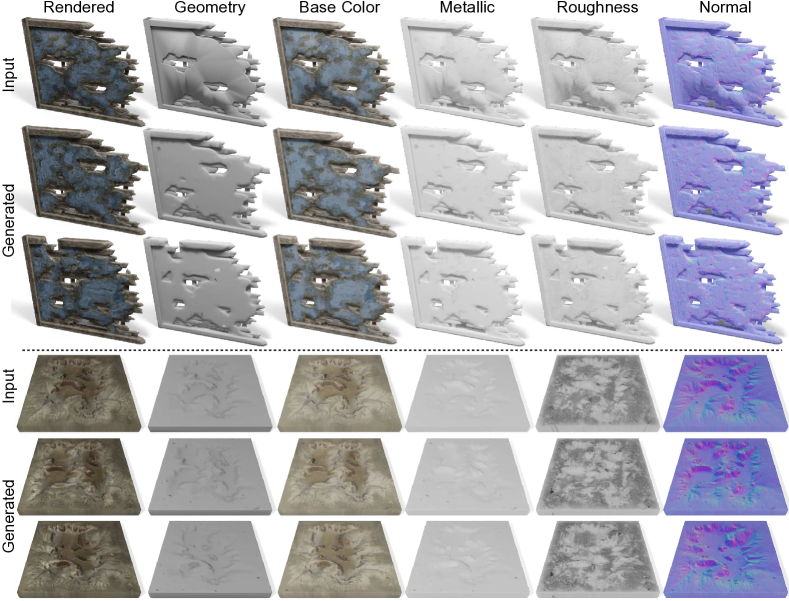
Figure 14. More results on 3D models with PBR material. Damaged wall (Max Ramirez, 2016), terrain (DJMaesen, 2018).

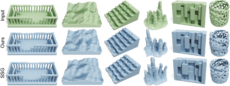
Figure 15. Visual comparison to SSG (Wu et al., 2016) on geometry generation. For most cases, our generated geometry are cleaner and sharper. But for examples with thin structures, our results are more likely to be broken (e.g., the vase).

References

- (1)
- 3ddominator (2019) 3ddominator. 2019. Train Wagon. https://sketchfab.com/3d-models/train-wagon-42875c098c33456b84bcfcdc4c7f1c58. License: CC Attribution.
- Achlioptas et al. (2018) Panos Achlioptas, Olga Diamanti, Ioannis Mitliagkas, and Leonidas Guibas. 2018. Learning representations and generative models for 3d point clouds. In International conference on machine learning. PMLR, 40–49.
- Ahmad Riazi (2013) Ahmad Riazi. 2013. Voronoi Card Stand. https://sketchfab.com/3d-models/voronoi-card-stand-9df4c3437f4c4db7bfaeda35cfc33c5f. License: CC Attribution.
- All-about-Blender-3D (2020) All-about-Blender-3D. 2020. Photo-realistic floating wood. https://www.cgtrader.com/free-3d-models/plant/other/photo-realistic-floating-wood. License: Royalty Free.
- Bokeloh et al. (2010) Martin Bokeloh, Michael Wand, and Hans-Peter Seidel. 2010. A connection between partial symmetry and inverse procedural modeling. In ACM SIGGRAPH 2010 papers. 1–10.
- Cai et al. (2020) Ruojin Cai, Guandao Yang, Hadar Averbuch-Elor, Zekun Hao, Serge Belongie, Noah Snavely, and Bharath Hariharan. 2020. Learning gradient fields for shape generation. In European Conference on Computer Vision. Springer, 364–381.
- Chan et al. (2021) Eric R Chan, Connor Z Lin, Matthew A Chan, Koki Nagano, Boxiao Pan, Shalini De Mello, Orazio Gallo, Leonidas Guibas, Jonathan Tremblay, Sameh Khamis, et al. 2021. Efficient geometry-aware 3D generative adversarial networks. arXiv preprint arXiv:2112.07945 (2021).
- Chang et al. (2015) Angel X. Chang, Thomas Funkhouser, Leonidas Guibas, Pat Hanrahan, Qixing Huang, Zimo Li, Silvio Savarese, Manolis Savva, Shuran Song, Hao Su, Jianxiong Xiao, Li Yi, and Fisher Yu. 2015. ShapeNet: An Information-Rich 3D Model Repository. Technical Report arXiv:1512.03012 [cs.GR]. Stanford University — Princeton University — Toyota Technological Institute at Chicago.
- Chen et al. (2021) Zhiqin Chen, Vladimir G Kim, Matthew Fisher, Noam Aigerman, Hao Zhang, and Siddhartha Chaudhuri. 2021. Decor-gan: 3d shape detailization by conditional refinement. In Proceedings of the IEEE/CVF Conference on Computer Vision and Pattern Recognition. 15740–15749.
- Chen et al. (2020) Zhiqin Chen, Andrea Tagliasacchi, and Hao Zhang. 2020. Bsp-net: Generating compact meshes via binary space partitioning. In Proceedings of the IEEE/CVF Conference on Computer Vision and Pattern Recognition. 45–54.
- Chen and Zhang (2019) Zhiqin Chen and Hao Zhang. 2019. Learning implicit fields for generative shape modeling. In Proceedings of the IEEE/CVF Conference on Computer Vision and Pattern Recognition. 5939–5948.
- Cheng et al. (2022) Yen-Chi Cheng, Hsin-Ying Lee, Sergey Tulyakov, Alexander Schwing, and Liangyan Gui. 2022. SDFusion: Multimodal 3D Shape Completion, Reconstruction, and Generation. arXiv preprint arXiv:2212.04493 (2022).
- choly kurd (2021) choly kurd. 2021. akropolis. https://www.turbosquid.com/3d-models/acropolis-3ds-free/610885. License: Educational Uses.
- Community (2018) Blender Online Community. 2018. Blender - a 3D modelling and rendering package. Blender Foundation, Stichting Blender Foundation, Amsterdam. http://www.blender.org
- Deitke et al. (2022) Matt Deitke, Dustin Schwenk, Jordi Salvador, Luca Weihs, Oscar Michel, Eli VanderBilt, Ludwig Schmidt, Kiana Ehsani, Aniruddha Kembhavi, and Ali Farhadi. 2022. Objaverse: A Universe of Annotated 3D Objects. arXiv preprint arXiv:2212.08051 (2022).
- Deyama (2018) Deyama. 2018. Temple ruins. https://sketchfab.com/3d-models/temple-ruins-6b3eb4e27e03485a886ce5304e95f897. License: CC Attribution.
- Dhariwal and Nichol (2021) Prafulla Dhariwal and Alexander Nichol. 2021. Diffusion models beat gans on image synthesis. Advances in Neural Information Processing Systems 34 (2021), 8780–8794.
- DJMaesen (2018) DJMaesen. 2018. Terrain 2. https://sketchfab.com/3d-models/terrain-2-29b795a7fe5c41e4b3ab7c91dc062cd7. License: CC Attribution.
- DJMaesen (2021) DJMaesen. 2021. Cliff. https://sketchfab.com/3d-models/cliff-082da1166a814c6e9c9e6c1b38159e4e. License: CC Attribution.
- Epic Games (2019) Epic Games. 2019. Unreal Engine. https://www.unrealengine.com
- Fridovich-Keil et al. (2022) Sara Fridovich-Keil, Alex Yu, Matthew Tancik, Qinhong Chen, Benjamin Recht, and Angjoo Kanazawa. 2022. Plenoxels: Radiance fields without neural networks. In Proceedings of the IEEE/CVF Conference on Computer Vision and Pattern Recognition. 5501–5510.
- Frybrix (2018) Frybrix. 2018. Minerals. https://sketchfab.com/3d-models/minerals-cab9d55faf0948b9a264d5550ee0f335. License: CC Attribution.
- Funkhouser et al. (2004) Thomas Funkhouser, Michael Kazhdan, Philip Shilane, Patrick Min, William Kiefer, Ayellet Tal, Szymon Rusinkiewicz, and David Dobkin. 2004. Modeling by example. ACM transactions on graphics (TOG) 23, 3 (2004), 652–663.
- Gao et al. (2022) Jun Gao, Tianchang Shen, Zian Wang, Wenzheng Chen, Kangxue Yin, Daiqing Li, Or Litany, Zan Gojcic, and Sanja Fidler. 2022. Get3d: A generative model of high quality 3d textured shapes learned from images. Advances In Neural Information Processing Systems 35 (2022), 31841–31854.
- Goodfellow et al. (2014) Ian Goodfellow, Jean Pouget-Abadie, Mehdi Mirza, Bing Xu, David Warde-Farley, Sherjil Ozair, Aaron Courville, and Yoshua Bengio. 2014. Generative Adversarial Nets. In Advances in Neural Information Processing Systems, Z. Ghahramani, M. Welling, C. Cortes, N. Lawrence, and K.Q. Weinberger (Eds.), Vol. 27. Curran Associates, Inc. https://proceedings.neurips.cc/paper/2014/file/5ca3e9b122f61f8f06494c97b1afccf3-Paper.pdf
- Granot et al. (2021) Niv Granot, Ben Feinstein, Assaf Shocher, Shai Bagon, and Michal Irani. 2021. Drop the gan: In defense of patches nearest neighbors as single image generative models. arXiv preprint arXiv:2103.15545 (2021).
- Greshler et al. (2021) Gal Greshler, Tamar Shaham, and Tomer Michaeli. 2021. Catch-A-Waveform: Learning to Generate Audio from a Single Short Example. In Advances in Neural Information Processing Systems, M. Ranzato, A. Beygelzimer, Y. Dauphin, P.S. Liang, and J. Wortman Vaughan (Eds.), Vol. 34. Curran Associates, Inc., 20916–20928.
- Gupta et al. (2023) Anchit Gupta, Wenhan Xiong, Yixin Nie, Ian Jones, and Barlas Oğuz. 2023. 3DGen: Triplane Latent Diffusion for Textured Mesh Generation. arXiv preprint arXiv:2303.05371 (2023).
- Haim et al. (2021) Niv Haim, Ben Feinstein, Niv Granot, Assaf Shocher, Shai Bagon, Tali Dekel, and Michal Irani. 2021. Diverse Generation from a Single Video Made Possible. arXiv preprint arXiv:2109.08591 (2021).
- Hertz et al. (2020) Amir Hertz, Rana Hanocka, Raja Giryes, and Daniel Cohen-Or. 2020. Deep Geometric Texture Synthesis. ACM Trans. Graph. 39, 4, Article 108 (2020). https://doi.org/10.1145/3386569.3392471
- Hinz et al. (2021) Tobias Hinz, Matthew Fisher, Oliver Wang, and Stefan Wermter. 2021. Improved techniques for training single-image gans. In Proceedings of the IEEE/CVF Winter Conference on Applications of Computer Vision. 1300–1309.
- Ho et al. (2020) Jonathan Ho, Ajay Jain, and Pieter Abbeel. 2020. Denoising diffusion probabilistic models. Advances in Neural Information Processing Systems 33 (2020), 6840–6851.
- ImpJive (2021) ImpJive. 2021. Fighting Pillar. https://sketchfab.com/3d-models/fighting-pillar-14e73d2d9e8a4981b49d0e6c56d30af5. License: CC Attribution-ShareAlike.
- Jayaraman et al. (2022) Pradeep Kumar Jayaraman, Joseph G Lambourne, Nishkrit Desai, Karl DD Willis, Aditya Sanghi, and Nigel JW Morris. 2022. SolidGen: An Autoregressive Model for Direct B-rep Synthesis. arXiv preprint arXiv:2203.13944 (2022).
- JB3D (2019) JB3D. 2019. Old towers in ruins. https://sketchfab.com/3d-models/pack-of-old-towers-in-ruins-f213359c6cbb4c29bf8880764faa0fb8. License: CC Attribution.
- Jones et al. (2020) R. Kenny Jones, Theresa Barton, Xianghao Xu, Kai Wang, Ellen Jiang, Paul Guerrero, Niloy J. Mitra, and Daniel Ritchie. 2020. ShapeAssembly: Learning to Generate Programs for 3D Shape Structure Synthesis. ACM Transactions on Graphics (TOG), Siggraph Asia 2020 39, 6 (2020), Article 234.
- Jun and Nichol (2023) Heewoo Jun and Alex Nichol. 2023. Shap-E: Generating Conditional 3D Implicit Functions. arXiv preprint arXiv:2305.02463 (2023).
- Kalogerakis et al. (2012) Evangelos Kalogerakis, Siddhartha Chaudhuri, Daphne Koller, and Vladlen Koltun. 2012. A probabilistic model for component-based shape synthesis. Acm Transactions on Graphics (TOG) 31, 4 (2012), 1–11.
- Karnewar et al. (2022) Animesh Karnewar, Oliver Wang, Tobias Ritschel, and Niloy J Mitra. 2022. 3inGAN: Learning a 3D generative model from images of a self-similar scene. In 2022 International Conference on 3D Vision (3DV). IEEE, 342–352.
- Kulikov et al. (2022) Vladimir Kulikov, Shahar Yadin, Matan Kleiner, and Tomer Michaeli. 2022. SinDDM: A Single Image Denoising Diffusion Model. arXiv preprint arXiv:2211.16582 (2022).
- Laetitia Irata (2019) Laetitia Irata. 2019. Temple of Ikov Reimagined. https://sketchfab.com/3d-models/temple-of-ikov-reimagined-b54f26e7807a4edeb2a84455c52b0cf6. License: CC Attribution.
- Laine et al. (2020) Samuli Laine, Janne Hellsten, Tero Karras, Yeongho Seol, Jaakko Lehtinen, and Timo Aila. 2020. Modular Primitives for High-Performance Differentiable Rendering. ACM Transactions on Graphics 39, 6 (2020).
- Li et al. (2017) Jun Li, Kai Xu, Siddhartha Chaudhuri, Ersin Yumer, Hao Zhang, and Leonidas Guibas. 2017. Grass: Generative recursive autoencoders for shape structures. ACM Transactions on Graphics (TOG) 36, 4 (2017), 1–14.
- Li et al. (2022) Peizhuo Li, Kfir Aberman, Zihan Zhang, Rana Hanocka, and Olga Sorkine-Hornung. 2022. GANimator: Neural Motion Synthesis from a Single Sequence. ACM Transactions on Graphics (TOG) 41, 4 (2022), 138.
- Li et al. (2021) Ruihui Li, Xianzhi Li, Ka-Hei Hui, and Chi-Wing Fu. 2021. SP-GAN: Sphere-guided 3D shape generation and manipulation. ACM Transactions on Graphics (TOG) 40, 4 (2021), 1–12.
- Li et al. (2023) Weiyu Li, Xuelin Chen, Jue Wang, and Baoquan Chen. 2023. Patch-based 3D Natural Scene Generation from a Single Example. (2023).
- Lin et al. (2023) Chen-Hsuan Lin, Jun Gao, Luming Tang, Towaki Takikawa, Xiaohui Zeng, Xun Huang, Karsten Kreis, Sanja Fidler, Ming-Yu Liu, and Tsung-Yi Lin. 2023. Magic3D: High-Resolution Text-to-3D Content Creation. In IEEE Conference on Computer Vision and Pattern Recognition (CVPR).
- Liu et al. (2023) Ruoshi Liu, Rundi Wu, Basile Van Hoorick, Pavel Tokmakov, Sergey Zakharov, and Carl Vondrick. 2023. Zero-1-to-3: Zero-shot One Image to 3D Object. arXiv preprint arXiv:2303.11328 (2023).
- Lorensen and Cline (1987) William E. Lorensen and Harvey E. Cline. 1987. Marching Cubes: A High Resolution 3D Surface Construction Algorithm (SIGGRAPH ’87). Association for Computing Machinery, New York, NY, USA, 163–169. https://doi.org/10.1145/37401.37422
- Loshchilov and Hutter (2017) Ilya Loshchilov and Frank Hutter. 2017. Decoupled weight decay regularization. arXiv preprint arXiv:1711.05101 (2017).
- Lukas carnota (2015) Lukas carnota. 2015. Industrial Building. https://www.cgtrader.com/free-3d-models/exterior/office/indusrtial-building. License: Royalty Free.
- Marti David Rial (2021) Marti David Rial. 2021. High detail sandstone mountain. https://www.cgtrader.com/items/2951688/download-page. License: Royalty Free.
- Max Ramirez (2016) Max Ramirez. 2016. Damaged Wall (PBR). https://sketchfab.com/3d-models/damaged-wall-pbr-009fc4bbc1184fca8fb6d6f15359d835. License: CC Attribution.
- Merrell (2007) Paul Merrell. 2007. Example-based model synthesis. In Proceedings of the 2007 symposium on Interactive 3D graphics and games. 105–112.
- Mescheder et al. (2019) Lars Mescheder, Michael Oechsle, Michael Niemeyer, Sebastian Nowozin, and Andreas Geiger. 2019. Occupancy Networks: Learning 3D Reconstruction in Function Space. In Proceedings of the IEEE/CVF Conference on Computer Vision and Pattern Recognition (CVPR).
- Metzer et al. (2022) Gal Metzer, Elad Richardson, Or Patashnik, Raja Giryes, and Daniel Cohen-Or. 2022. Latent-NeRF for Shape-Guided Generation of 3D Shapes and Textures. arXiv preprint arXiv:2211.07600 (2022).
- Mildenhall et al. (2020) Ben Mildenhall, Pratul P. Srinivasan, Matthew Tancik, Jonathan T. Barron, Ravi Ramamoorthi, and Ren Ng. 2020. NeRF: Representing Scenes as Neural Radiance Fields for View Synthesis. In ECCV.
- Mo et al. (2019) Kaichun Mo, Paul Guerrero, Li Yi, Hao Su, Peter Wonka, Niloy Mitra, and Leonidas J Guibas. 2019. Structurenet: Hierarchical graph networks for 3d shape generation. arXiv preprint arXiv:1908.00575 (2019).
- Nash et al. (2020) Charlie Nash, Yaroslav Ganin, SM Ali Eslami, and Peter Battaglia. 2020. Polygen: An autoregressive generative model of 3d meshes. In International Conference on Machine Learning. PMLR, 7220–7229.
- Nichol et al. (2022) Alex Nichol, Heewoo Jun, Prafulla Dhariwal, Pamela Mishkin, and Mark Chen. 2022. Point-E: A System for Generating 3D Point Clouds from Complex Prompts. arXiv preprint arXiv:2212.08751 (2022).
- Nikankin et al. (2022) Yaniv Nikankin, Niv Haim, and Michal Irani. 2022. SinFusion: Training Diffusion Models on a Single Image or Video. arXiv preprint arXiv:2211.11743 (2022).
- nikola (2020) nikola. 2020. Low poly trees. https://sketchfab.com/3d-models/low-poly-trees-a00c46d6a1a149e2b1f4b6dbf4767a4d. License: CC Attribution.
- oguzhnkr (2017) oguzhnkr. 2017. Antique Pillar. https://sketchfab.com/3d-models/antique-pillar-ab3730246f1e4598b4704fae747d7d56. License: CC Attribution.
- Park et al. (2019) Jeong Joon Park, Peter Florence, Julian Straub, Richard Newcombe, and Steven Lovegrove. 2019. Deepsdf: Learning continuous signed distance functions for shape representation. In Proceedings of the IEEE/CVF Conference on Computer Vision and Pattern Recognition. 165–174.
- Pavllo et al. (2021) Dario Pavllo, Jonas Kohler, Thomas Hofmann, and Aurelien Lucchi. 2021. Learning Generative Models of Textured 3D Meshes from Real-World Images. In Proceedings of the IEEE/CVF International Conference on Computer Vision. 13879–13889.
- Pedram Ashoori (2020) Pedram Ashoori. 2020. Small Town. https://www.cgtrader.com/free-3d-models/exterior/cityscape/small-town-87b127c8-c991-4063-aa69-e58800686299. License: Royalty Free.
- Peng et al. (2020) Songyou Peng, Michael Niemeyer, Lars Mescheder, Marc Pollefeys, and Andreas Geiger. 2020. Convolutional occupancy networks. In European Conference on Computer Vision. Springer, 523–540.
- Poole et al. (2022) Ben Poole, Ajay Jain, Jonathan T. Barron, and Ben Mildenhall. 2022. DreamFusion: Text-to-3D using 2D Diffusion. arXiv (2022).
- Raab et al. (2023) Sigal Raab, Inbal Leibovitch, Guy Tevet, Moab Arar, Amit H Bermano, and Daniel Cohen-Or. 2023. Single Motion Diffusion. arXiv preprint arXiv:2302.05905 (2023).
- Ramesh et al. (2022) Aditya Ramesh, Prafulla Dhariwal, Alex Nichol, Casey Chu, and Mark Chen. 2022. Hierarchical text-conditional image generation with clip latents. arXiv preprint arXiv:2204.06125 (2022).
- REÂRCH Studio (2018) REÂRCH Studio. 2018. Palisade Wall. https://sketchfab.com/3d-models/palisade-wall-low-poly-1bb195ca9fd4468da3ea4fbedcc4b77f. License: CC Attribution.
- Rombach et al. (2022) Robin Rombach, Andreas Blattmann, Dominik Lorenz, Patrick Esser, and Björn Ommer. 2022. High-resolution image synthesis with latent diffusion models. In Proceedings of the IEEE/CVF Conference on Computer Vision and Pattern Recognition. 10684–10695.
- Ruiz et al. (2022) Nataniel Ruiz, Yuanzhen Li, Varun Jampani, Yael Pritch, Michael Rubinstein, and Kfir Aberman. 2022. Dreambooth: Fine tuning text-to-image diffusion models for subject-driven generation. arXiv preprint arXiv:2208.12242 (2022).
- Saharia et al. (2022) Chitwan Saharia, William Chan, Saurabh Saxena, Lala Li, Jay Whang, Emily L Denton, Kamyar Ghasemipour, Raphael Gontijo Lopes, Burcu Karagol Ayan, Tim Salimans, et al. 2022. Photorealistic text-to-image diffusion models with deep language understanding. Advances in Neural Information Processing Systems 35 (2022), 36479–36494.
- Schuhmann et al. (2022) Christoph Schuhmann, Romain Beaumont, Richard Vencu, Cade Gordon, Ross Wightman, Mehdi Cherti, Theo Coombes, Aarush Katta, Clayton Mullis, Mitchell Wortsman, et al. 2022. Laion-5b: An open large-scale dataset for training next generation image-text models. arXiv preprint arXiv:2210.08402 (2022).
- Shaham et al. (2019) Tamar Rott Shaham, Tali Dekel, and Tomer Michaeli. 2019. Singan: Learning a generative model from a single natural image. In Proceedings of the IEEE/CVF International Conference on Computer Vision. 4570–4580.
- Shahriar Shahrabi (2021) Shahriar Shahrabi. 2021. The Vast Land. https://sketchfab.com/3d-models/the-vast-land-733b802f5a4743ef99ad574279d49920. License: CC Attribution.
- Shocher et al. (2019) Assaf Shocher, Shai Bagon, Phillip Isola, and Michal Irani. 2019. Ingan: Capturing and retargeting the” dna” of a natural image. In Proceedings of the IEEE/CVF International Conference on Computer Vision. 4492–4501.
- Shue et al. (2022) J Ryan Shue, Eric Ryan Chan, Ryan Po, Zachary Ankner, Jiajun Wu, and Gordon Wetzstein. 2022. 3D Neural Field Generation using Triplane Diffusion. arXiv preprint arXiv:2211.16677 (2022).
- skinny hands (2021) skinny hands. 2021. Stylized Stone Tiles. https://sketchfab.com/3d-models/stylized-stone-tiles-ce62cfea8caa49eb8b579944bd99b311. License: CC Attribution.
- SLASH / RENDAR (2020) SLASH / RENDAR. 2020. Industrial Pipe. https://sketchfab.com/3d-models/old-industrial-pipe-pack-pbr-a10a6011334e4d11a7023d67705ac1d4. License: CC Attribution.
- Sohl-Dickstein et al. (2015) Jascha Sohl-Dickstein, Eric Weiss, Niru Maheswaranathan, and Surya Ganguli. 2015. Deep unsupervised learning using nonequilibrium thermodynamics. In International Conference on Machine Learning. PMLR, 2256–2265.
- Son et al. (2022) Minjung Son, Jeong Joon Park, Leonidas Guibas, and Gordon Wetzstein. 2022. SinGRAF: Learning a 3D Generative Radiance Field for a Single Scene. arXiv preprint arXiv:2211.17260 (2022).
- Song et al. (2020) Jiaming Song, Chenlin Meng, and Stefano Ermon. 2020. Denoising diffusion implicit models. arXiv preprint arXiv:2010.02502 (2020).
- stray (2015) stray. 2015. Wooden irregular wall. https://www.cgtrader.com/free-3d-models/architectural/engineering/wooden-irregular-wall. License: Royalty Free.
- Wang et al. (2022b) Haochen Wang, Xiaodan Du, Jiahao Li, Raymond A Yeh, and Greg Shakhnarovich. 2022b. Score Jacobian Chaining: Lifting Pretrained 2D Diffusion Models for 3D Generation. arXiv preprint arXiv:2212.00774 (2022).
- Wang et al. (2022c) Tengfei Wang, Bo Zhang, Ting Zhang, Shuyang Gu, Jianmin Bao, Tadas Baltrusaitis, Jingjing Shen, Dong Chen, Fang Wen, Qifeng Chen, et al. 2022c. Rodin: A Generative Model for Sculpting 3D Digital Avatars Using Diffusion. arXiv preprint arXiv:2212.06135 (2022).
- Wang et al. (2022a) Weilun Wang, Jianmin Bao, Wengang Zhou, Dongdong Chen, Dong Chen, Lu Yuan, and Houqiang Li. 2022a. SinDiffusion: Learning a Diffusion Model from a Single Natural Image. arXiv preprint arXiv:2211.12445 (2022).
- Werniech (2022) Werniech. 2022. Large Stone Arch. https://www.turbosquid.com/3d-models/large-stone-arch-3d-1908101. License: TurboSquid Standard License.
- Werniech van der Heever (2019) Werniech van der Heever. 2019. Stalagmites. https://www.cgtrader.com/free-3d-models/various/various-models/stalagmites-2c2dd36e-76bc-449e-85ba-c38376e646a3. License: Royalty Free.
- Wu et al. (2016) Jiajun Wu, Chengkai Zhang, Tianfan Xue, Bill Freeman, and Josh Tenenbaum. 2016. Learning a probabilistic latent space of object shapes via 3d generative-adversarial modeling. Advances in neural information processing systems 29 (2016).
- Wu et al. (2021) Rundi Wu, Chang Xiao, and Changxi Zheng. 2021. Deepcad: A deep generative network for computer-aided design models. In Proceedings of the IEEE/CVF International Conference on Computer Vision. 6772–6782.
- Wu and Zheng (2022) Rundi Wu and Changxi Zheng. 2022. Learning to Generate 3D Shapes from a Single Example. ACM Transactions on Graphics (TOG) 41, 6 (2022), 1–19.
- Xu et al. (2012) Kai Xu, Hao Zhang, Daniel Cohen-Or, and Baoquan Chen. 2012. Fit and diverse: Set evolution for inspiring 3d shape galleries. ACM Transactions on Graphics (TOG) 31, 4 (2012), 1–10.
- Yang et al. (2019) Guandao Yang, Xun Huang, Zekun Hao, Ming-Yu Liu, Serge Belongie, and Bharath Hariharan. 2019. Pointflow: 3d point cloud generation with continuous normalizing flows. In Proceedings of the IEEE/CVF International Conference on Computer Vision. 4541–4550.
- Young (2023) Jonathan Young. 2023. xatlas. https://github.com/jpcy/xatlas.
- Zeng et al. (2022) Xiaohui Zeng, Arash Vahdat, Francis Williams, Zan Gojcic, Or Litany, Sanja Fidler, and Karsten Kreis. 2022. LION: Latent Point Diffusion Models for 3D Shape Generation. In Advances in Neural Information Processing Systems, Vol. 35. Curran Associates, Inc., 10021–10039.
- Zhang et al. (2018) Richard Zhang, Phillip Isola, Alexei A Efros, Eli Shechtman, and Oliver Wang. 2018. The Unreasonable Effectiveness of Deep Features as a Perceptual Metric. In CVPR.
- Zhang et al. (2021) ZiCheng Zhang, CongYing Han, and TianDe Guo. 2021. ExSinGAN: Learning an explainable generative model from a single image. arXiv preprint arXiv:2105.07350 (2021).
- Zhang et al. (2022) Zhixing Zhang, Ligong Han, Arnab Ghosh, Dimitris Metaxas, and Jian Ren. 2022. SINE: SINgle Image Editing with Text-to-Image Diffusion Models. arXiv preprint arXiv:2212.04489 (2022).
- Šimon Ustal (2020) Šimon Ustal. 2020. Canyon Landscape. https://sketchfab.com/3d-models/canyon-landscape-c395e9eb54ba4f40820ccfb98d3c2832. License: CC Attribution.