Differentially-Private Decision Trees and Provable Robustness to Data Poisoning

Abstract

Decision trees are interpretable models that are well-suited to non-linear learning problems. Much work has been done on extending decision tree learning algorithms with differential privacy, a system that guarantees the privacy of samples within the training data. However, current state-of-the-art algorithms for this purpose sacrifice much utility for a small privacy benefit. These solutions create random decision nodes that reduce decision tree accuracy or spend an excessive share of the privacy budget on labeling leaves. Moreover, many works do not support continuous features or leak information about them. We propose a new method called PrivaTree based on private histograms that chooses good splits while consuming a small privacy budget. The resulting trees provide a significantly better privacy-utility trade-off and accept mixed numerical and categorical data without leaking information about numerical features. Finally, while it is notoriously hard to give robustness guarantees against data poisoning attacks, we demonstrate bounds for the expected accuracy and success rates of backdoor attacks against differentially-private learners. By leveraging the better privacy-utility trade-off of PrivaTree we are able to train decision trees with significantly better robustness against backdoor attacks compared to regular decision trees and with meaningful theoretical guarantees.

I Introduction

Machine learning has achieved widespread success with neural networks and ensemble methods, but it is almost impossible for humans to understand the decisions such models make [1]. Fortunately, much work has been done on training machine learning models that are directly interpretable by humans [2]. Especially size-limited decision trees [3, 4] are successful methods for their interpretability combined with their ability to predict non-linear data.

While decision trees can offer interpretability, they reveal information about the data they were trained on. This is a detrimental property when models are trained on private data that contains sensitive information, such as in fraud detection and medical applications. Differentially-private [5] machine learning models solve this problem by introducing carefully crafted randomness into the way the models are trained [6]. For differentially-private decision trees, the entire model consisting of decision node splits and leaf labels can be made public, and by extension, predictions made by the model. This is not only useful for training interpretable private models, but decision trees are also vital primitives for building ensembles [7, 8, 9, 10] for tabular data. The key problem in training differentially-private models is efficiently spending the privacy budget $\epsilon$ to achieve high utility. In this work, we propose an algorithm for training decision trees with an improved privacy-utility trade-off.

Many previous works have already proposed ways to generate differentially-private decision trees, but they also have shortcomings. There are two main categories of algorithms here. The first category [11, 12, 13, 14] chooses splits completely at random and allocates the entire privacy budget for labeling the leaves. The second category [15, 16, 17, 18] extends the greedy splitting procedure of regular decision trees, where splits are selected by optimizing a splitting criterion. These works guarantee differential privacy by incorporating noise into the splitting criterion while consuming a part of the user-defined privacy budget. However, naive approaches require computing many scores resulting in consuming privacy budget frequently and using up much budget to select good decision nodes. The remaining budget is spent on labeling leaves.

In this work, we propose a method called PrivaTree to train differentially-private decision trees. PrivaTree uses the privacy budget much more efficiently than previous work when choosing splits by leveraging private histograms. We also propose a strategy for distributing the privacy budget that offers good performance for both very small and large datasets. The result is a practical method for training private trees with a significantly better utility. PrivaTree also prevents leakage from the location of splits on numerical features, a property that some previous methods do not have. Moreover, we demonstrate how the ability to train accurate differentially-private decision trees with small privacy budgets allows for performance guarantees against data poisoning attacks in which an adversary manipulates the training data. Our experiments on various tabular benchmark datasets demonstrate an improved privacy-utility trade-off compared to other private trees. We also experimentally demonstrate that PrivaTree offers stronger poisoning robustness guarantees than private logistic regression [19], another interpretable method. Our experiments on the MNIST 0 vs 1 dataset show that indeed PrivaTrees with small privacy budgets resist a trigger-based backdoor attack.

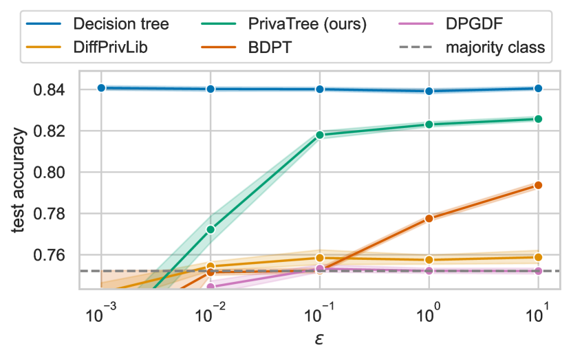
(a) adult dataset (45222 samples, 14 features)

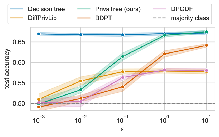
(b) compas-two-years (4966 samples, 11 features)

Figure 1: Mean accuracy scores of depth 4 trees when varying privacy budget $\epsilon$ from private to less private with 50 repetitions. For extremely small privacy budgets DiffPrivLib performs best but for higher budgets, PrivaTree achieves a significantly higher accuracy.

II Preliminaries

II-A Decision tree learning

Decision trees are simple models that consist of nodes that apply logical rules to a sample, and leaves that hold a prediction. By simply following a path through the rules one ends up in a leaf of which the value is predicted. Decision trees have become a popular choice of model due to their straight-forward interpretation when limiting the size of the tree [1] and their success in more complex ensembles [7, 8, 9, 10, 20]. While it is debatable what exact tree size maintains interpretability, we choose to train trees up to a depth of 4 resulting in at most 16 leaves.

The most popular algorithms for learning decision trees are based on CART [3] and ID3 [4]. For classification tasks, these algorithms recursively create decision nodes that minimize Gini impurity or maximize information gain and create leaves labeled with the majority of labels that reach them. While these methods are greedy heuristics and thus offer few guarantees [21], they perform well in practice. Due to the success of decision trees in gradient boosting, much effort has gone into implementing efficient algorithms using histograms [9, 10]. We base PrivaTree on such histogram-based learners, but where the choice of histograms in boosting was motivated by runtime efficiency we leverage them to achieve a better trade-off between privacy and accuracy.

II-B Differential privacy

Differential privacy [5, 22, 23] provides strong privacy guarantees for algorithms over aggregate datasets, which implies that the existence of any record in the dataset does not influence the output probability with factors $\epsilon$ and $\delta$. This property prevents membership attacks, attacks aimed at determining whether specific samples were included in the train set of a model, with a high probability if $\epsilon$ is chosen small enough.

Definition 1 (Differential privacy).

A randomized algorithm $\mathcal{M}$ satisfies $(\epsilon,\delta)$-differential privacy if for all neighboring datasets $\mathcal{D},\mathcal{D}^{\prime}\in\mathbb{N}^{|\mathcal{X}|}$ differing in one element, and any $\mathcal{S}\subseteq\mathrm{Range}(\mathcal{M})$,

$$\Pr[\mathcal{M}(\mathcal{D})\in\mathcal{S}]\leq e^{\epsilon}\Pr[\mathcal{M}(\mathcal{D}^{\prime})\in\mathcal{S}]+\delta$$ (1)

where $\mathbb{N}$ is the set of non-negative integers and $\mathcal{X}$ is the universe for all datasets. If $\delta$ is $0$, $\mathcal{M}$ satisfies $\epsilon$-differential privacy.

Among differentially private mechanisms, the Laplace mechanism adds noise to a numerical output, and the exponential mechanism returns a precise output among a group according to the utility scores for each element. Both mechanisms are widely used and are defined as follows.

Definition 2 (Laplace mechanism [22]).

A randomized algorithm $\mathcal{M}$ satisfies $\epsilon$-differential privacy over a real value query $f:\mathbb{N}^{|\mathcal{X}|}\rightarrow\mathbb{R}^{k}$ if

$$\mathcal{M}(\mathcal{D},\ f,\ \epsilon)=f(\mathcal{D})+(y_{1}\ \dots\ y_{k})\ ,\ \ \ \ \ y_{i}\sim\mathrm{Lap}\left(\frac{\Delta f}{\epsilon}\right)$$ (2)

where $\mathrm{Lap}(b)$ is the Laplace distribution with scale $b$ that $\mathrm{Lap}(x\ |\ b)=\frac{1}{2b}\exp(-\frac{|x|}{b})$, and $\Delta f$ is the ${l}_{1}$-sensitivity that

$$\Delta f=\max\limits_{X,X^{\prime}\in\mathbb{N}^{|\mathcal{X}|},||X-X^{\prime}||_{1}\leq 1}||f(X)-f(X^{\prime})||_{1}$$ (3)

With the Laplace mechanism, the Laplace noise is added to the accurate output of the query $f$ so that the output of $\mathcal{M}$ satisfies $\epsilon$-differential privacy over the query. Other mechanisms, such as the Gaussian mechanism and geometric mechanism [24], achieve differential privacy in a similar way. The geometric mechanism is similar to the Laplace mechanism but works with integer values. An algorithm $\mathcal{M}(\mathcal{D},\ f,\ \epsilon)$ is $\epsilon$-differentially private when the noise follows the two-sided geometric distribution:

$$\Pr[y_{i}=\delta]=\frac{1-\epsilon}{1+\epsilon}\epsilon^{|\delta|}$$ (4)

with a query $f$, the parameter $\epsilon\in(0,1)$ and every integer $\delta$.

Definition 3 (Exponential mechanism [25]).

A randomized algorithm $\mathcal{M}$ satisfies $\epsilon$-differential privacy over a utility function $u:\mathbb{N}^{|\mathcal{X}|}\times\mathcal{R}\rightarrow\mathbb{R}$ if $\mathcal{M}$ selects an element $t\in\mathcal{R}$ with the probability that

$$\Pr[\mathcal{M} (\mathcal{D},u,\epsilon,\mathcal{R})=t\in\mathcal{R}]=$$ (5)

$$\frac{\exp{(\epsilon u(\mathcal{D},t)/(2\Delta u)})\cdot\mu(t)}{\sum_{r\in\mathcal{R}}\exp{((\epsilon u(\mathcal{D},r)/(2\Delta u))}\cdot\mu(r)}$$

where $\Delta u$ is the sensitivity that

$$\Delta u=\max\limits_{r\in\mathcal{R}}\max\limits_{X,X^{\prime}\in\mathbb{N}^{|\mathcal{X}|},||X-X^{\prime}||_{1}\leq 1}|u(X,r)-u(X^{\prime},r)|$$ (6)

where $\mathcal{R}$ is the range for output, and $\mu$ is a measure over $\mathcal{R}$.

In contrast to the Laplace mechanism, the exponential mechanism assigns a probability to each possible output in the group according to the utility score. By doing that, the mechanism can output a precise element using the probabilities, and perturbation is added for the selection procedure. Similarly, permute-and-flip [26] randomly chooses a value from a set of options, weighed by a utility score and the privacy parameter $\epsilon$. For each possible output, the mechanism simulates flipping a biased coin, and the item is returned if the head is up with a probability according to an exponential function. Otherwise, it flips the coin for the next item with new probabilities assigned. Compared to the exponential mechanism, the probability of outputting an item is updated for each round, and the authors of [26] also show that the permute-and-flip mechanism never performs worse than the exponential mechanism in expectation and better in other situations.

Meanwhile, differential privacy holds sequential and parallel composition properties [27] as shown in Theorems 1 and 2. For a series of mechanisms $\mathcal{M}_{[k]}=(\mathcal{M}_{1},\dots,\mathcal{M}_{k})$, each $\mathcal{M}_{i}$ is $\epsilon_{i}$-differentially private for $i\in[k]$. The sequential composition indicates that $(\sum_{i}\epsilon_{i})$-differential privacy is guaranteed if the series of mechanisms are applied sequentially to the input, and the parallel composition implies that $(\max_{i}\epsilon_{i})$-differential privacy is achieved if the series of mechanisms are applied to different disjoint subsets of the input.

Theorem 1 (Sequential composition).

If mechanism $\mathcal{M}_{i}$ is $\epsilon_{i}$-differentially private, the sequence of $\mathcal{M}_{[k]}(X)$ provides $(\sum_{i}\epsilon_{i})$-differential privacy.

Theorem 2 (Parallel composition).

If mechanism $\mathcal{M}_{i}$ is $\epsilon_{i}$-differentially private, and $\mathcal{D}_{i}$ are disjoint subsets of the input domain $\mathcal{D}$, the sequence of $\mathcal{M}_{[k]}(X\cap\mathcal{D}_{i})$ provides $(\max_{i}\epsilon_{i})$-differential privacy.

The privacy parameter $\epsilon$ is often referred to as the privacy budget as it can be intuitively interpreted this way. Following the intuition a private algorithm has a total budget of $\epsilon$ that it can spend on composed operations. Operations that get little budget will return noisier results than operations with much budget so by composing operations in parallel when possible and by carefully distributing the budget over the operations one can achieve a good trade-off between privacy and utility.

II-C Poisoning robustness

Data poisoning attacks are attacks in which a malicious actor adds, removes, or modifies the data that a machine learning model is trained on. By making specific changes to the dataset, attackers can for example reduce the model’s performance or plant a backdoor that allows the attacker to inject a specific ’trigger pattern’ into an input of the model at test time to control its prediction. While much work has gone into defending against poisoning attacks [28, 29, 30] and into provable robustness against other attacks such as evasion [31, 32] it is notoriously difficult to provide provable guarantees on poisoning defenses. In this work, we demonstrate the provable poisoning robustness of differentially-private decision trees. We discuss existing methods for certified poisoning robustness in section III-B.

TABLE I: Overview of methods for training differentially private decision trees, algorithms marked with * use smooth sensitivity. Most methods use the exponential mechanism $\mathcal{M}_{EM}$ for splitting and $\mathcal{M}_{\text{Laplace}}$ for labeling leaves. Methods without splitting a mechanism use random trees.

Method			Features		Mechanism
Name	Year	Ref	Cat.	Num.	Splitting	Labeling
SuLQ ID3	2005	[15]	●	○	$\mathcal{M}_{\text{Gaussian}}$	$\mathcal{M}_{\text{Gaussian}}$
Private-RDT	2009	[14]	●	●	-	$\mathcal{M}_{\text{Laplace}}$
SuLQ-based ID3	2010	[18]	●	●	$\mathcal{M}_{\text{Laplace}}$	$\mathcal{M}_{\text{Laplace}}$
DiffPID3	2010	[18]	●	●	$\mathcal{M}_{EM}$	$\mathcal{M}_{\text{Laplace}}$
DiffGen	2011	[33]	●	●	$\mathcal{M}_{EM}$	$\mathcal{M}_{\text{Laplace}}$
DT-Diff	2013	[34]	●	●	$\mathcal{M}_{EM}$	$\mathcal{M}_{\text{Laplace}}$
dpRFMV/dpRFTA	2014	[11]	●	●	-	$\mathcal{M}_{\text{Laplace}}$
DPDF	2015	[17]	●	○	$\mathcal{M}_{EM}$	$\mathcal{M}_{\text{Laplace}}$
Rana et al.	2015	[35]	●	●	$\mathcal{M}_{\text{Laplace}}$	$\mathcal{M}_{\text{Laplace}}$
Smooth Random	2017	[12]	●	●	-	$\mathcal{M}_{EM}$*
ADiffP	2018	[16]	●	○	$\mathcal{M}_{EM}$	$\mathcal{M}_{\text{Laplace}}$
DPGDF	2019	[36]	●	○	$\mathcal{M}_{EM}$	$\mathcal{M}_{EM}$*
BDPT	2020	[37]	●	●	$\mathcal{M}_{EM}$*	$\mathcal{M}_{\text{Laplace}}$
TrainSingleTree	2020	[38]	○	●	$\mathcal{M}_{EM}$	$\mathcal{M}_{\text{Laplace}}$
DiffPrivLib	2021	[13]	○	●	-	$\mathcal{M}_{PF}$
PrivaTree	This work		●	●	$\mathcal{M}_{\text{Geometric}}$	$\mathcal{M}_{PF}$

III Related work

III-A Differentially-private decision tree learning

Many previous works already propose algorithms for training differentially-private decision trees. These algorithms address the privacy leakage in regular trees by replacing the node splitting and leaf labeling operations with differentially-private alternatives. This paper only considers algorithms for single decision trees. Fletcher and Islam [39] wrote a survey on this topic which also examines ensembles such as in private boosting [40].

Table I provides a summary of existing algorithms for training private decision trees. In the ‘features’ column, we indicate whether the algorithm considers categorical and numerical features. We remark that algorithms for numerical splits can also support categories using one-hot encoding, and algorithms for categories can heuristically support numerical features by applying binning. Note that unless computed using differential privacy, the resulting bins reveal information about the training data. In that case, the model only guarantees differential privacy for the leaves, which is equivalent to labelDP [41]. The mechanism columns of the table indicate the private mechanisms used for node splitting and leaf labeling. Besides the specific choice of mechanism, the way these mechanisms are sequentially applied and the way the privacy budget is distributed have a significant effect on the algorithm’s performance.

There are two main categories of algorithms for training differentially-private trees. The first category trains random decision trees, that replace split searching by splitting uniformly at random from the domain of possible feature values. A benefit of doing so is that splitting does not depend on the data and does not consume any privacy budget so labeling can be performed with the comeplete budget. However, random splits do not necessarily produce good leaves as having worse splits leads to leaves that contain a mix of samples from all classes. As a result, accurate labels will still cause misclassifications. For certain datasets, the poor quality of random splits strongly affects the performance of the resulting tree. For this reason, random decision trees are almost exclusively used in ensembles. Examples of such algorithms are Private-RDT [14], dpRFMV/dpRFTA [11], Smooth Random Trees [12] and the implementation of DiffPrivLib trees [13].

The second category consists of algorithms that train a greedy tree by probabilistically choosing a split weighed by a scoring function such as the information gain or the Gini impurity. SuLQ ID3 [15] and SuLQ-based ID3 [18] do so by adding Gaussian or Laplace noise to the scores themselves, while works like DiffPID3 [18], DiffGen [33], DT-Diff [34] and TrainSingleTree [38] do so not by perturbing the scores, but using the exponential mechanism so the privacy budget does not have to be divided over so many queries. DPDF [17] further increases the utility of the queries by bounding the sensitivity of the Gini impurity, while ADiffP [16] dynamically allocates the privacy budget.

We compare against three of the latest algorithms for training private trees. BDPT [37] is a greedy tree algorithm that uses the exponential mechanism for splitting but with smooth sensitivity, allowing for a higher utility per query as compared to previous works. DPGDF [36] is a similar algorithm that uses smooth sensitivity for creating the leaves rather than the splits. This algorithm only support categorical features. Finally, DiffPrivLib [13] offers a recent implementation of random trees. For the leaves it uses the permute-and-flip mechanism, which performs better in practice than the exponential mechanism [26]. This algorithm only supports numerical features.

III-B Provable poisoning robustness

While it is difficult to provide strong guarantees for poisoning robustness, several works have done so in the past. Steinhardt et al. [42] remove outliers based on metrics such as distance from the centroid of a class and can formally guarantee the accuracy of convex learners under specific poisoning attacks. Rosenfeld et al. [43] consider label-flipping attacks in which only the labels can be changed by the attacker. They certify robust prediction of specific test samples for linear models by giving a bound on the minimum number of training labels that have to be flipped to change the test sample’s prediction. Deep Partition Aggregation (DPA) [44] trains an ensemble on disjoint subsets of the training dataset such that each sample is seen by only one member of the ensemble. Then, for a specific test sample, one can compute a bound on the number of train samples that should be perturbed to flip the prediction. These previous methods do not apply to single decision tree models.

Several works have guaranteed robustness using differential privacy. Ma et al. [45] prove general bounds on the attack cost for varying numbers of poisoned samples and apply this analysis to logistic regression. Also, several works have used differentially-private neural networks to be more robust against poisoning attacks [46, 47, 48], sometimes even demonstrating robustness in configurations in which the theoretical guarantees do not apply. Compared to DPA, differential privacy guarantees robustness of a global metric such as accuracy while methods like DPA guarantee robust predictions for each test sample individually.

While multiple works have considered the poisoning robustness of differentially-private learners, to the best of our knowledge there is no demonstration of strong robustness guarantees for single decision trees. Drews et al. [49] do analyze the robustness of regular non-private decision tree learners but show that for trees of depth 4 only 4 samples are often enough to reduce the accuracy guarantees to 0. As we will demonstrate, private decision trees with a good privacy-utility trade-off can guarantee poisoning robustness and outperform logistic regression in this regard. For the sake of completeness, we also compare against DPA [44] which uses decision trees inside its ensemble to offer strong guarantees, but sacrifices interpretability and privacy.

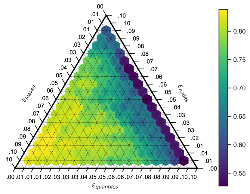
(a) vote dataset (435 samples, 16 features)

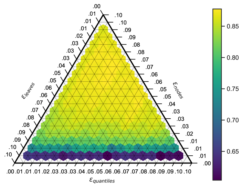
(b) pol dataset (10082 samples, 26 features)

Figure 2: Training accuracy scores when varying the distribution of the privacy budget $\epsilon=0.1$ over different parts of the PrivaTree algorithm with depth 3. Scores were averaged over 50 executions. On small datasets such as vote, the best trees allocate more budget to the leaves, while large datasets such as pol benefit from more budget for splitting.

IV Improving differentially private decision trees: PrivaTree

In this section, we present PrivaTree, which is an algorithm for training differentially-private decision trees with high utility. PrivaTree incorporates three techniques to improve performance:

• Private histograms to find good splits using the Gini impurity with reduced spending of privacy budget.

• A better distribution of privacy budget based on a bound for labeling leaves accurately.

• The permute-and-flip mechanism instead of the exponential mechanism for leaf labeling and the Geometric instead of the Laplace mechanism for node splitting.

Additionally, PrivaTree uses a pre-processing technique based on private quantiles which enables it to train on both numerical and categorical features. PrivaTree assumes that the range of numerical features, the set of categorical values, the set of class labels, and the dataset size are publicly known. We provide pseudocode in Algorithm 1, which we describe in more detail in the rest of this section.

IV-A Scoring splits using private histograms

Classification tree learning algorithms such as CART create decision nodes by recursively choosing a split among all feature values that minimizes the weighted Gini impurity. Previous differentially-private decision trees used similar approaches but often leak information about numerical feature values. Friedman and Schuster [18] show how to privately split on numerical features using the continuous exponential mechanism but this requires more privacy budget because each feature needs to be considered separately. Another work, BDPT, permits some leakage, providing a weaker form of privacy by averaging every 5 numerical feature values, and then splitting using the exponential mechanism.

Numerical features

To find high-quality splits while protecting feature value information and efficiently using the privacy budget, we use private histograms. Splitting according to histograms has been a successful progression in decision tree learning for gradient boosting ensembles [9, 10] where it is used for its runtime efficiency. Instead, we rely on them because they only require noise to be added once per bin (parallel composition), allowing us to only add noise once for each node. Specifically, we add noise with the Geometric mechanism over the Laplace mechanism since histogram counts are integers and we use privacy budget $\epsilon_{\text{node,num}}$ which we define later. In the rest of this paper, we fix the number of bins for numerical features to 10. To find a split, the PrivaTree algorithm computes a private histogram for each class and for each feature, computes the Gini impurity of the split between every bin, and selects the split that minimizes impurity. This results in decision node rules of the kind ‘feature value $\leq$ threshold’.

Categorical features

Previous decision tree learning algorithms support categorical features by only splitting one category at a time. While this method is sound, it often requires deep trees to make enough splits for categorical features to be useful, and this harms interpretability. In the PrivaTree algorithm, we find a locally optimal partition of the categories instead. Such rules are of the kind ‘categories $L$ go left, categories $R$ go right’. As a result of Coppersmith et al. [50], this partition is efficiently identified for binary classification by first sorting the categories by their ratio of class 0 versus class 1 members followed by the typical splitting procedure. To guarantee differential privacy we perform the sort operation based on the private histogram with privacy budget $\epsilon_{\text{node,cat}}$. For the multiclass case, we simply keep the order of categories as supplied by the user.

IV-B Pre-processing by private quantiles

Before the splitting procedure, PrivaTree needs to select the boundaries of the 10 bins of the private histograms for each numerical feature. A natural choice is to create equal-width bins of numerical features based on the public knowledge of each feature’s range, but there is a problem with this approach: features with long tails would cause data to be concentrated in a few bins and would result in a large loss of information. Instead, we bin numerical features using quantiles so that they evenly divide the samples over each bin. Since regular quantiles leak information about the dataset, we resort to differentially-private quantiles. We use the jointexp algorithm [51] for this, which improves performance over optimal statistical estimation techniques [52] when computing multiple quantiles on the same data. This algorithm runs with privacy budget $\epsilon_{\text{quantile}}$ which we define later. Categorical variables require no pre-processing. Instead, we encode them as integers and the split-finding operation handles these values natively.

IV-C Leaf labeling according to majority votes

Once the PrivaTree algorithm has produced a series of decision nodes by recursively splitting and reaches the stopping criterion, the algorithm creates a leaf containing a prediction. In the non-private setting, the prediction is usually chosen to be the majority of the class labels of samples that reach that leaf to maximize accuracy. However, this leaks private information. Previous works have used the Laplace or (smooth) exponential mechanisms but like modern implementations such as DiffPrivLib [13] we opt for the permute-and-flip mechanism [26]. Permute-and-flip is proven to have an expected error that is at least as good or better than that of the exponential mechanism and practically outperforms it. To label a leaf we therefore count the number of samples of each class and apply permute-and-flip with privacy budget $\epsilon_{\text{leaf}}$ which we define later.

Algorithm 1 Train PrivaTree with $\epsilon$ differential privacy

Input: dataset $X$ ($n\times m$), labels $y$, privacy budget $\epsilon$, maximum leaf error $\mathcal{E}_{max}$, maximum depth $d$

1:$\epsilon_{\text{leaf}}=\min(\frac{\epsilon}{2},\epsilon^{\prime}_{\text{leaf}})$, where $\epsilon^{\prime}_{\text{leaf}}$ is computed with Equation 7

2:$\epsilon_{\text{node,num}}=\epsilon_{\text{quantiles}}=(\epsilon-\epsilon_{\text{leaf}})\cdot\frac{1}{1+d}$,  $\epsilon_{\text{node,cat}}=(\epsilon-\epsilon_{\text{leaf}})\cdot\frac{1}{d}$

3:for numerical features $j_{\text{num}}$ do

4:     bin values $X_{i,j_{\text{num}}}$ into bins $B_{j_{\text{num}}}$ determined by quantiles with jointexp [51]$\triangleright$ with budget $\epsilon_{\text{quantiles}}$

5:end for

6:procedure FitTree($X^{\prime},y^{\prime},d^{\prime}$)

7:     if $d^{\prime}$ = $0$ or $|X^{\prime}_{i,j}|\leq 1$ or $y^{\prime}$ contains a single class then

8:         compute class counts $N_{0},N_{1},...,N_{K}$ for all $K$ classes

9:         return $\text{Leaf}(\mathcal{M}_{PF}(\langle N_{0},N_{1},...,N_{K}\rangle))$ $\triangleright$ with budget $\epsilon_{\text{leaf}}$

10:     else

11:         Create histograms $\forall j,k,b{\in}B_{j}:H_{j,b,k}\leftarrow\mathcal{M}_{\text{Geometric}}(\sum_{i}[X^{\prime}_{i,j}{=}b\land y^{\prime}_{i}{=}k])$ $\triangleright$ with budget $\epsilon_{\text{node,num}}$ or $\epsilon_{\text{node,cat}}$

12:         find split $(j^{*},b^{*})$ that minimizes Gini impurity w.r.t. histograms $H_{j,b,k}$

13:         partition $X^{\prime}$ into $(X^{\text{left}},X^{\text{right}})$, and $y^{\prime}$ into $(y^{\text{left}},y^{\text{right}})$ according to $(j^{*},b^{*})$

14:         $\mathcal{T}_{\text{left}}\leftarrow$ FitTree($X^{\text{left}},y^{\text{left}},d^{\prime}{-}1$),  $\mathcal{T}_{\text{right}}\leftarrow$ FitTree($X^{\text{right}},y^{\text{right}},d^{\prime}{-}1$)

15:         return Node$(j^{*},b^{*},\mathcal{T}_{\text{left}},\mathcal{T}_{\text{right}})$

16:     end if

17:end procedure

18:return FitTree($X,y,d$)

IV-D Distributing the privacy budget

The composability property of differential privacy allows modular algorithm design by breaking up the algorithm into differentially-private primitives. However, it is generally not obvious how to distribute the privacy budget $\epsilon$ over the primitives to maximize the expected utility of the outcomes. Previous works have tried various heuristics such as distributing $\epsilon$ equally over each private operation or distributing epsilon 50-50 between node and leaf operations. To understand the role of budget distribution in private tree learning we visualized the average training accuracy over 50 runs when varying budget spent on each part of the algorithm (quantile finding, node splitting and leaf labeling) in Figure 2. We find that when $\epsilon$ is large compared to the dataset size this results in excess budget being spent on leaf labeling where it could have improved node selection. By noticing that we can bound the expected error incurred by labeling leaves for a given privacy budget, we propose a budget distribution scheme that scales well for varying values of $\epsilon$. When the privacy budget is low compared to the dataset size, set $\epsilon_{\text{leaf}}=\frac{\epsilon}{2}$, i.e. half of the budget. When the budget is relatively high, set $\epsilon_{\text{leaf}}$ such that the maximum expected error incurred by labeling $\mathbb{E}[\mathcal{E}(\mathcal{M},\vec{N})]$ is at most equal to the user-specified labeling error limit $\mathcal{E}_{max}$. Distribute the remaining budget $\epsilon-\epsilon_{\text{leaf}}$ uniformly over quantile and node operations to improve algorithm utility for higher values of $\epsilon$. For all our results we used $\mathcal{E}_{max}=0.01$, i.e. if possible only allow an extra accuracy loss of 1% due to leaf labeling.

Corollary 1.

For $K$ classes, $n$ samples and depth $d$ trees, the amount of privacy budget $\epsilon^{\prime}_{\text{leaf}}$ needed for labeling leaves with the permute-and-flip mechanism with expected error $\mathbb{E}[\mathcal{E}(\mathcal{M}_{PF},\vec{N})]$ of at most $\mathcal{E}_{max}$ is:

$$\epsilon^{\prime}_{\mathrm{leaf}}\leq\frac{2^{d}\max_{p}2\log(\frac{1}{p})\left(1-\frac{1-(1-p)^{K}}{Kp}\right)}{n\;\mathcal{E}_{max}}\;,$$ (7)

Proof.

This result naturally follows from applying the worst-case error bound proved for $\mathcal{M}_{PF}$ in the permute-and-flip paper [26]. A complete proof is given in the appendix. ∎

Following the definition of $\epsilon^{\prime}_{\mathrm{leaf}}$ this results in the privacy budget being distributed as

$$\epsilon_{\text{leaf}} =\min\left(\frac{\epsilon}{2},\epsilon^{\prime}_{\text{leaf}}\right),$$ (8)

$$\epsilon_{\text{node,num}}=\epsilon_{\text{quantiles}} =\frac{\epsilon-\epsilon_{\text{leaf}}}{1+d},$$ (9)

$$\epsilon_{\text{node,cat}} =\frac{\epsilon-\epsilon_{\text{leaf}}}{d}.$$ (10)

Next, we show that this budget distribution scheme actually provides differential privacy by showing that the composition of mechanisms spends privacy budget equal to $\epsilon$.

Theorem 3.

PrivaTree, as described in Algorithm 1, provides $\epsilon$-differential privacy.

Proof.

For numerical attributes in the training set $X$, PrivaTree first computes the quantiles with $\epsilon_{\text{quantiles}}$. This can be done with parallel composition for each feature. After that, the algorithm recursively splits the root node and since each split creates two distinct partitions of the data, each data point is only used in $d$ nodes where $d$ is the maximum depth of the tree. The amount of budget spent on numerical node splitting is then $d\cdot\epsilon_{\text{node,num}}$ through sequential composition. Finally, leaf labeling consumes $\epsilon_{\text{leaf}}$ of the privacy budget and since each data point is only used in a single leaf this follows parallel composition (spending $\epsilon_{\text{leaf}}$ once). Combining all the operations we find that the amount of privacy budget spent for numerical features is:

$$\epsilon_{\text{num}} =\epsilon_{\text{quantiles}}+d\cdot\epsilon_{\text{node,num}}+\epsilon_{\text{leaf}}$$

$$=\frac{\epsilon-\epsilon_{\text{leaf}}}{1+d}+d\cdot\frac{\epsilon-\epsilon_{\text{leaf}}}{1+d}+\epsilon_{\text{leaf}}$$

$$=\frac{(1+d)(\epsilon-\epsilon_{\text{leaf}})}{1+d}+\epsilon_{\text{leaf}}$$

$$=\epsilon-\epsilon_{\text{leaf}}+\epsilon_{\text{leaf}}$$

$$=\epsilon.$$

For categorical attributes in $X$, there is no need to calculate the quantiles. Therefore categorical feature node splitting takes privacy budget $d\cdot\epsilon_{\text{node,cat}}$, and leaf labeling takes budget $\epsilon_{\text{leaf}}$. The overall privacy parameter for categorical attributes follows similarly to that of numerical attributes:

$$\epsilon_{\text{cat}} =d\cdot\epsilon_{\text{node,cat}}+\epsilon_{\text{leaf}}$$

$$=d\cdot\frac{\epsilon-\epsilon_{\text{leaf}}}{d}+\epsilon_{\text{leaf}}$$

$$=\epsilon-\epsilon_{\text{leaf}}+\epsilon_{\text{leaf}}$$

$$=\epsilon.$$

Since numerical and categorical attributes are disjoint subsets of the input dataset $X$ they follow parallel composition and therefore Algorithm 1 provides $\max(\epsilon_{\text{num}},\epsilon_{\text{cat}})=\max(\epsilon,\epsilon)=\epsilon$-differential privacy. ∎

V Poisoning Robustness

When using machine learning trained on crowd-sourced data, such as in federated learning scenarios, or on potentially manipulated data one has to consider malicious user behavior. One such threat is data poisoning, in which users insert $x$ data points into the training dataset to confuse the classifier or introduce a backdoor. Many defenses have been proposed such as using learning behavior to ignore backdoor data [53] or post-processing based on adversarial robustness to remove backdoors [54] but such methods work heuristically and offer no guarantees. We use the fact that $\epsilon$-differentially-private machine learning algorithms are limited in sensitivity to dataset changes to provide guarantees against poisoning attacks. Ma et al. [45] introduce the attack cost $J(D)=\mathbb{E}[C(\mathcal{M}(D))]$, i.e. the expected value of a cost function $C$ that an attacker gets from models produced by $\mathcal{M}$ on dataset $D$. They prove the following about the cost of attacks against differentially-private learners:

Theorem 4.

[45] Let $\mathcal{M}$ be an $\epsilon$-differentially-private learner. Let $J(\tilde{D})$ be the attack cost, where $\tilde{D}\ominus D\leq x$ (i.e. a dataset with $x$ poisoned samples compared to clean dataset $D$), then

$$J(\tilde{D}) \geq e^{-x\epsilon}J(D),\quad(C\geq 0)$$ (11)

$$J(\tilde{D}) \geq e^{x\epsilon}J(D).\quad(C\leq 0)$$ (12)

We will consider two scenarios with different attacker objectives and their associated cost functions:

• An attacker adds or removes up to $x$ samples from a dataset in an attempt to maximally reduce the accuracy of a model learned from the dataset. The associated cost function is the accuracy of the model, i.e. $J_{\text{Acc}}(\tilde{D})=\mathbb{E}[\text{Accuracy}(\mathcal{M}(\tilde{D}))]$.

• An attacker adds $x$ copies of data points with a trigger pattern inserted into them and the associated label is changed to a target label in an effort to create a backdoor. The associated cost function is the Attack Success Rate (ASR), i.e. the percentage of data points for which the predicted label can be flipped to the target label. Since Theorem 4 assumes (without loss of generality) that the attacker minimizes $J$, we use the complement of the ASR as the cost, as the attacker wants to maximize ASR: $J_{\text{ASR}}(\tilde{D})=\mathbb{E}[1-\text{ASR}(\mathcal{M}(\tilde{D}))]$.

These two settings lead to the following robustness guarantees that we empirically evaluate in Section VI for various private learners and datasets.

Corollary 2.

Let $\mathcal{M}$ be an $\epsilon$-differentially-private learner. Let $J_{\text{Acc}}(\tilde{D})=\mathbb{E}[\text{Accuracy}(\mathcal{M}(\tilde{D}))]$ be the model’s expected accuracy on the poisoned dataset $\tilde{D}$, where $\tilde{D}\in B(D,x)$ (i.e. a dataset with $x$ poisoned samples), then

$$\mathbb{E}[\text{Accuracy}(\mathcal{M}(\tilde{D}))]\geq e^{-x\epsilon}\;\mathbb{E}[\text{Accuracy}(\mathcal{M}(D))]$$

Proof.

Since the accuracy score function is non-negative this follows directly from Equation 11:

$$J(\tilde{D}) \geq e^{-x\epsilon}J(D)$$

$$\mathbb{E}[\text{Accuracy}(\mathcal{M}(\tilde{D}))] \geq e^{-x\epsilon}\;\mathbb{E}[\text{Accuracy}(\mathcal{M}(D))]\;.\qed$$

Corollary 3.

Let $\mathcal{M}$ be an $\epsilon$-differentially-private learner. Let $J_{\text{ASR}}(\tilde{D})=\mathbb{E}[1-\text{ASR}(\mathcal{M}(\tilde{D}))]$ be the expected backdoor attack success rate on the poisoned dataset $\tilde{D}$, where $\tilde{D}\in B(D,x)$ (i.e. a dataset with $x$ poisoned samples), then

$$\mathbb{E}[\text{ASR}(\mathcal{M}(\tilde{D}))]\leq 1-e^{-x\epsilon}\;\mathbb{E}[1-\text{ASR}(\mathcal{M}(D))]$$

Proof.

Since $J_{\text{ASR}}$ is non-negative we derive the guarantee from Equation 11:

$$J(\tilde{D}) \geq e^{-x\epsilon}J(D)$$

$$\mathbb{E}[1-\text{ASR}(\mathcal{M}(\tilde{D}))] \geq e^{-x\epsilon}\;\mathbb{E}[1-\text{ASR}(\mathcal{M}(D))]$$

$$\mathbb{E}[\text{ASR}(\mathcal{M}(\tilde{D}))]-\mathbb{E}[1] \leq-e^{-x\epsilon}\;\mathbb{E}[1-\text{ASR}(\mathcal{M}(D))]$$

$$\mathbb{E}[\text{ASR}(\mathcal{M}(\tilde{D}))] \leq 1-e^{-x\epsilon}\;\mathbb{E}[1-\text{ASR}(\mathcal{M}(D))]\;.\qed$$

TABLE II: 5-fold cross-validated mean test accuracy and standard errors at $\epsilon{=}0.1$ for trees of depth 4. PrivaTree* ran without private quantile computation, DPGDF only ran on categorical features. PrivaTree outperforms existing methods on most datasets.

OpenML dataset	decision tree	BDPT	PrivaTree*	DPGDF	DiffPrivLib	PrivaTree
	no privacy	leaking numerical splits		differential privacy
Numerical data
Bioresponse	.701 $\pm$ .009	.502 $\pm$ .001	.574 $\pm$ .015	-	.519 $\pm$ .013	.564 $\pm$ .017
Diabetes130US	.606 $\pm$ .002	.511 $\pm$ .005	.601 $\pm$ .001	-	.507 $\pm$ .003	.600 $\pm$ .001
Higgs	.657 $\pm$ .001	timeout	.658 $\pm$ .001	-	.513 $\pm$ .010	.659 $\pm$ .001
MagicTelescope	.783 $\pm$ .008	.500 $\pm$ .000	.756 $\pm$ .003	-	.553 $\pm$ .022	.740 $\pm$ .005
MiniBooNE	.872 $\pm$ .001	.500 $\pm$ .000	.859 $\pm$ .002	-	.509 $\pm$ .006	.858 $\pm$ .002
bank-marketing	.768 $\pm$ .004	.501 $\pm$ .001	.735 $\pm$ .008	-	.538 $\pm$ .013	.747 $\pm$ .008
california	.783 $\pm$ .002	.500 $\pm$ .000	.754 $\pm$ .009	-	.512 $\pm$ .005	.756 $\pm$ .006
covertype	.741 $\pm$ .001	.502 $\pm$ .001	.745 $\pm$ .002	-	.569 $\pm$ .035	.748 $\pm$ .001
credit	.748 $\pm$ .001	.500 $\pm$ .000	.739 $\pm$ .003	-	.516 $\pm$ .009	.720 $\pm$ .014
default-of-credit-card-clients	.700 $\pm$ .006	.500 $\pm$ .000	.679 $\pm$ .008	-	.549 $\pm$ .019	.684 $\pm$ .003
electricity	.731 $\pm$ .001	.500 $\pm$ .000	.738 $\pm$ .003	-	.555 $\pm$ .030	.736 $\pm$ .006
eye_movements	.571 $\pm$ .010	.500 $\pm$ .000	.532 $\pm$ .007	-	.518 $\pm$ .007	.514 $\pm$ .009
heloc	.702 $\pm$ .004	.518 $\pm$ .009	.696 $\pm$ .002	-	.532 $\pm$ .015	.677 $\pm$ .011
house_16H	.819 $\pm$ .003	.500 $\pm$ .000	.765 $\pm$ .010	-	.555 $\pm$ .009	.769 $\pm$ .007
jannis	.718 $\pm$ .001	.500 $\pm$ .000	.707 $\pm$ .003	-	.564 $\pm$ .032	.702 $\pm$ .003
pol	.930 $\pm$ .001	.509 $\pm$ .014	.871 $\pm$ .011	-	.580 $\pm$ .016	.836 $\pm$ .015
Numerical & categorical data
albert	.641 $\pm$ .002	.501 $\pm$ .001	.632 $\pm$ .002	.511 $\pm$ .008	.546 $\pm$ .017	.631 $\pm$ .003
compas-two-years	.664 $\pm$ .005	.562 $\pm$ .013	.639 $\pm$ .007	.571 $\pm$ .004	.569 $\pm$ .005	.595 $\pm$ .013
covertype	.756 $\pm$ .001	.614 $\pm$ .001	.755 $\pm$ .001	.537 $\pm$ .011	.539 $\pm$ .018	.755 $\pm$ .001
default-of-credit.	.704 $\pm$ .005	.500 $\pm$ .001	.691 $\pm$ .005	.528 $\pm$ .004	.535 $\pm$ .015	.689 $\pm$ .006
electricity	.732 $\pm$ .002	.500 $\pm$ .000	.740 $\pm$ .004	.518 $\pm$ .004	.527 $\pm$ .014	.734 $\pm$ .004
eye_movements	.570 $\pm$ .003	.500 $\pm$ .001	.514 $\pm$ .007	.523 $\pm$ .004	.524 $\pm$ .009	.533 $\pm$ .005
road-safety	.728 $\pm$ .001	.685 $\pm$ .002	.710 $\pm$ .003	.685 $\pm$ .002	.555 $\pm$ .033	.721 $\pm$ .001
UCI datasets (numerical & categorical)
adult	.840 $\pm$ .001	.752 $\pm$ .000	.815 $\pm$ .001	.753 $\pm$ .002	.757 $\pm$ .003	.820 $\pm$ .003
breast-w	.950 $\pm$ .007	.614 $\pm$ .025	.909 $\pm$ .025	-	.842 $\pm$ .037	.886 $\pm$ .019
diabetes	.723 $\pm$ .012	.624 $\pm$ .017	.659 $\pm$ .011	-	.667 $\pm$ .010	.673 $\pm$ .019
mushroom	.977 $\pm$ .005	.880 $\pm$ .013	.973 $\pm$ .011	.761 $\pm$ .042	.749 $\pm$ .048	.985 $\pm$ .002
nursery	1.000 $\pm$ .000	1.000 $\pm$ .000	1.000 $\pm$ .000	.707 $\pm$ .027	.767 $\pm$ .061	1.000 $\pm$ .000
vote	.944 $\pm$ .014	.608 $\pm$ .062	.771 $\pm$ .081	.561 $\pm$ .081	.827 $\pm$ .036	.737 $\pm$ .061

TABLE III: 5-fold cross-validated mean test accuracy and poisoning accuracy guarantee against a percentage of poisoned samples on numerical datasets. Stronger privacy provides stronger poisoning robustness but comes at the cost of clean dataset accuracy. PrivaTree outperforms private logistic regression on this benchmark.

				poison guarantee
dataset	method	$\epsilon$	acc.	0.1%	0.5%	1%
Bioresponse	PrivaTree	.01	.522	.511	.458	.398
		.1	.545	.446	.149	.037
	diffprivlib LR	.01	.539	.528	.473	.411
		.1	.539	.442	.147	.036
Diabetes130US	PrivaTree	.01	.568	.324	.033	.002
		.1	.600	.002	.000	.000
	diffprivlib LR	.01	.516	.295	.030	.002
		.1	.528	.002	.000	.000
Higgs	PrivaTree	.01	.646	.000	.000	.000
		.1	.659	.000	.000	.000
	diffprivlib LR	.01	.496	.000	.000	.000
		.1	.592	.000	.000	.000
MagicTelescope	PrivaTree	.01	.652	.590	.384	.224
		.1	.738	.271	.004	.000
	diffprivlib LR	.01	.598	.541	.352	.205
		.1	.662	.243	.003	.000
MiniBooNE	PrivaTree	.01	.764	.428	.042	.002
		.1	.852	.003	.000	.000
	diffprivlib LR	.01	.418	.234	.023	.001
		.1	.491	.001	.000	.000
bank-marketing	PrivaTree	.01	.564	.521	.371	.243
		.1	.733	.329	.011	.000
	diffprivlib LR	.01	.480	.443	.315	.207
		.1	.578	.260	.009	.000
california	PrivaTree	.01	.699	.595	.308	.134
		.1	.762	.154	.000	.000
	diffprivlib LR	.01	.509	.434	.224	.098
		.1	.564	.114	.000	.000
covertype	PrivaTree	.01	.729	.008	.000	.000
		.1	.747	.000	.000	.000
	diffprivlib LR	.01	.574	.006	.000	.000
		.1	.615	.000	.000	.000

				poison guarantee
dataset	method	$\epsilon$	acc.	0.1%	0.5%	1%
credit	PrivaTree	.01	.536	.471	.277	.142
		.1	.725	.198	.001	.000
	diffprivlib LR	.01	.464	.408	.240	.123
		.1	.526	.143	.001	.000
default-of-credit.	PrivaTree	.01	.552	.499	.325	.191
		.1	.676	.249	.003	.000
	diffprivlib LR	.01	.506	.458	.298	.175
		.1	.560	.206	.003	.000
electricity	PrivaTree	.01	.670	.496	.145	.031
		.1	.732	.036	.000	.000
	diffprivlib LR	.01	.484	.358	.105	.022
		.1	.505	.025	.000	.000
eye_movements	PrivaTree	.01	.507	.477	.375	.278
		.1	.515	.283	.026	.001
	diffprivlib LR	.01	.511	.481	.378	.280
		.1	.503	.276	.025	.001
heloc	PrivaTree	.01	.593	.547	.397	.266
		.1	.681	.306	.012	.000
	diffprivlib LR	.01	.534	.493	.358	.240
		.1	.524	.236	.010	.000
house_16H	PrivaTree	.01	.615	.556	.362	.211
		.1	.751	.276	.004	.000
	diffprivlib LR	.01	.489	.442	.288	.168
		.1	.499	.184	.002	.000
jannis	PrivaTree	.01	.634	.400	.064	.006
		.1	.705	.007	.000	.000
	diffprivlib LR	.01	.482	.304	.048	.005
		.1	.569	.006	.000	.000
pol	PrivaTree	.01	.580	.535	.389	.261
		.1	.859	.386	.016	.000
	diffprivlib LR	.01	.477	.440	.320	.214
		.1	.635	.285	.012	.000

VI Results

We compare the performance of PrivaTree with regular decision trees from Scikit-learn [55] and 3 previous methods for training private decision trees: DiffPrivLib [13], BDPT [37] and DPGDF [36]. DiffPrivLib is a widely used Python library for differential privacy and implements several private machine learning models. Their decision tree implementation creates random decision nodes and uses all privacy budget to label leaves using the permute-and-flip mechanism. Since DiffPrivLib and Scikit-learn do not natively support categorical features we encode these into integers. BDPT and DPGDF did not share their implementations so we implemented these using primitives from DiffPrivLib. Since DPGDF only supports categorical variables we run experiments as in the work of Borhan [16] and remove numerical features. BDPT only heuristically protects numerical feature values so we compare it against PrivaTree* a variant of PrivaTree where we compute quantiles non-privately, and set $\epsilon_{\text{quantile}}=0$ and $\epsilon_{\text{node,num}}=(\epsilon-\epsilon_{\text{leaf}})\cdot\frac{1}{d}$.

We also compare the performance of PrivaTree on poisoning robustness with differentially-private logistic regression and Deep Partition Aggregation (DPA). Previous works on poisoning robustness with differential privacy have used private logistic regression [19] as a robust interpretable model. We use the implementation by DiffPrivLib [13] which perturbs the optimal model parameters. Before training, we center the data and normalize it to unit variance as this improves optimization. DPA trades interpretability and privacy for strong poisoning robustness guarantees by ensembling many models trained on distinct data subsets. We implement DPA with 1000 decision trees as tree-based models generally work better than neural networks for tabular data [20].

All experiments ran on a computer with 16GB of RAM and a 2 GHz Intel i5 processor with 4 cores. See our code for more details.

VI-A Predictive performance

To compare PrivaTree to existing works we evaluated performance on two well-known benchmarks. First, we experimented on 6 datasets from the UCI repository [56] that previous works tested on. However, these datasets are often small (diabetes), too easy to predict (nursery), or imbalanced (adult), which skews performance numbers. To complement this, we therefore also run experiments on the tabular data benchmark [20]. These datasets were chosen to be real-world, balanced, not too small, and not too simple. We removed rows with missing values and computed the public feature ranges based on the datasets, the categorical values are supplied by OpenML [57].

In Table II we present the accuracy scores on both benchmarks for trees of depth 4 computed with 5-fold stratified cross-validation at a privacy budget of $\epsilon=0.1$. Results for other budgets are given in the appendix. Since all private algorithms are based on the greedy algorithm for decision trees, the goal is to score similarly to the non-private trees. On almost all datasets PrivaTree outperforms BDPT, DPGDF, and DiffPrivLib or performs similarly. On breast-w and vote however, DiffPrivLib sometimes performs better. This is because, on such small datasets, it is better to avoid spending the privacy budget on good decision nodes and instead spend all budget on labeling leaves correctly. On most datasets, there is only a difference in score of a few percentage points between PrivaTree and PrivaTree*. BDPT has previously only been tested on numerical features with few unique values and fails to train accurate trees on the numerical tabular benchmark. In Figure 1 we visualize the average accuracy over 50 runs when varying the total privacy budget $\epsilon$ for depth 4 trees on the adult and compas-two-years datasets. Again, on very small $\epsilon$ values DiffPrivLib outperforms the other methods. However, as soon as there is enough privacy budget to see value from choosing better decision nodes (around $\epsilon{=}0.005$ and $\epsilon{=}0.05$ in the figure respectively) PrivaTree dominates the rest of the methods.

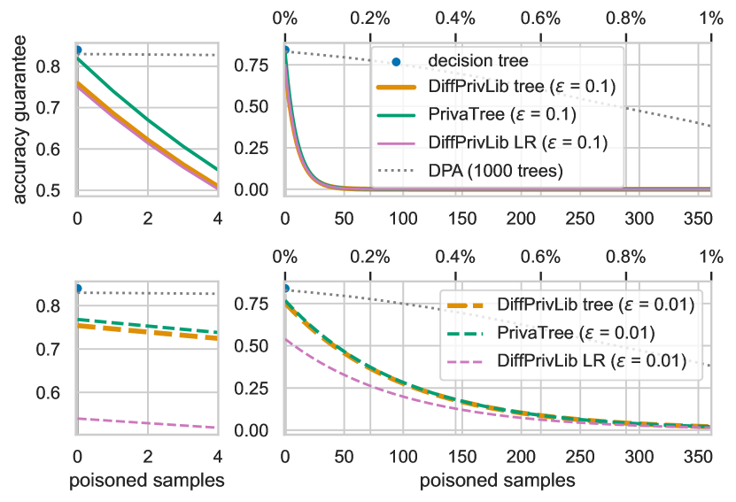
(a) adult dataset (45222 samples, 14 features)

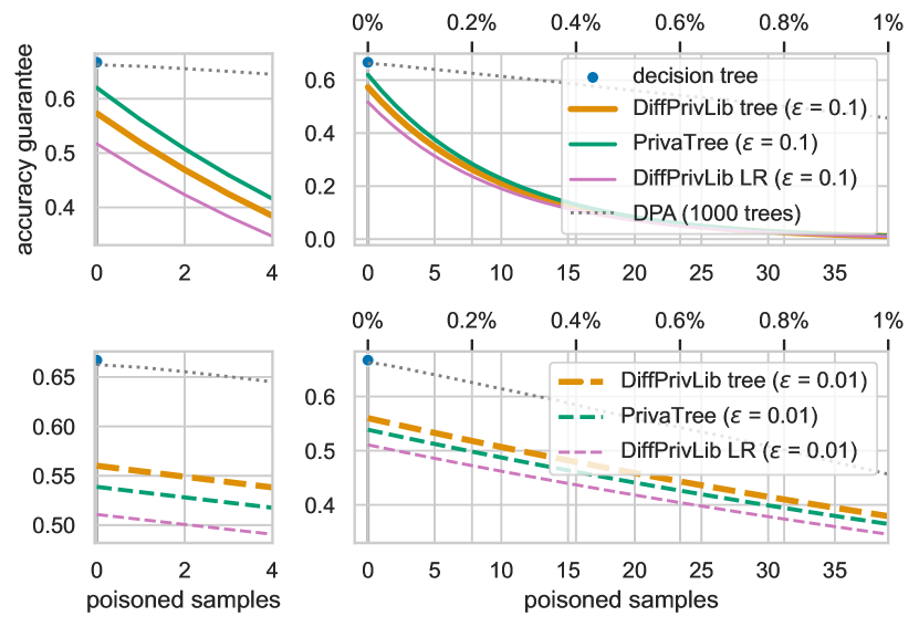
(b) compas-two-years (4966 samples, 11 features)

Figure 3: Guaranteed accuracy when varying the number of poisoned samples to up to 1% of the dataset size for trees of depth 4. A DPA ensemble of 1000 trees offers strong guarantees but is not interpretable nor does it maintain privacy. For differentially-private learners, there is a trade-off between clean accuracy and the quality of the robustness guarantee.

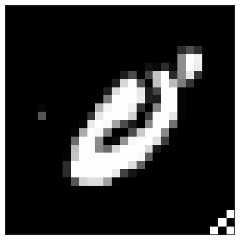
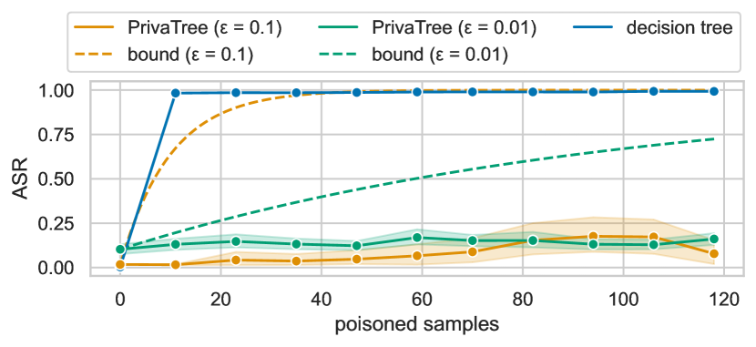
Figure 4: An adversary injects zeros with a trigger pattern to create a backdoor for class 1. (left) Poisoned sample of a 0 labeled as 1 with a trigger in the bottom-right. (right) The attack success rate when varying the number of poisoned samples in MNIST 0 vs 1 out of 11,200 train samples. $\epsilon{=}0.01$ offers a tighter bound than $\epsilon{=}0.1$ but in practice, both values defend well against the backdoor attack on this dataset.

VI-B Poisoning robustness guarantees for tabular data

Recall from Section V that differentially-private learners offer guarantees on the loss of accuracy incurred by attackers who poison the training dataset. In Figure 3, we visualized the guaranteed accuracy when varying the number of poisoned sampled in the dataset from 0% to 1% of the original train set size. These guarantees were determined by estimating the expected test accuracy with 50 random train-test splits and then computing the guarantees with Corollary 2. For comparison, we visualize the guarantee for DPA with an ensemble of 1000 depth 4 trees, but this method does not protect privacy and is not interpretable. The strength of the poisoning robustness guarantee for private learners is determined largely by the choice of $\epsilon$ and to a lesser extent the accuracy on the clean dataset. Therefore, there is an important trade-off between clean data accuracy and robustness guarantee.

Since previous works have considered the poisoning robustness guarantees of private logistic regression as an interpretable model, we compare against this method in more detail. In Table III, we display the accuracy and guarantees at various poison levels for private logistic regression and PrivaTree. We evaluated the models on numerical datasets as this will prevent differences in performance due to the way categorical features are encoded for logistic regression and PrivaTree. Results on data with categorical features can be found in the appendix. It is clear that there is a trade-off between accuracy and poison guarantee for both methods as guarantees at levels of 0.1% data poisoning are already always better when $\epsilon=0.01$, whereas test accuracy is always better when $\epsilon=0.1$. PrivaTrees outperform private logistic regression at equal privacy levels as these complex datasets likely contain non-linear patterns that are better captured by decision trees. Therefore, in the future, one should consider private decision trees as an alternative to private logistic regression when learning interpretable models with poisoning robustness guarantees.

VI-C Backdoor robustness on MNIST

To demonstrate the effectiveness of differentially private decision tree learners at mitigating data poisoning attacks, we evaluated backdoor attacks on the MNIST 0 vs 1 dataset. Specifically, we repeat the experiment from Badnets [58] in which the adversary adds a fixed trigger pattern to the bottom right corner of the image in an attempt to force zeros to be classified as ones. To achieve this, the adversary copies $x$ zeros, adds the trigger pattern to these images, and adds the copies to the training set with label 1. An example of a zero with a trigger pattern is shown in Figure 4. To measure the robustness of models against the backdoor, we compute the Attack Success Rate (ASR), which is the percentage of test samples with label 0 that are predicted as 1 when the trigger pattern is added. In Figure 4, we plot the ASR of a regular decision tree and PrivaTrees with privacy budgets 0.1 and 0.01 and their bounds computed with Corollary 3 against a varying number of poisoned samples ranging between 0% to 1% of the dataset. All trees were trained on 50 train-test splits and had a depth of 4. With only 0.01% of the train set poisoned, regular decision trees already suffer from an ASR of almost 100% whereas PrivaTrees on average stay at an ASR of under 20% for the entire range. While the bound for $\epsilon=0.01$ is much tighter than the bound for $\epsilon=0.1$, PrivaTrees perform well in practice for both settings.

Strong privacy and robustness guarantees come at the cost of utility, i.e. clean dataset accuracy. The test accuracy scores without poisoned samples for the models in Figure 4 were 99.5% for the regular decision tree, 98.7% for PrivaTree with $\epsilon{=}0.1$, and 97.4% for PrivaTree with $\epsilon{=}0.01$.

VII Discussion

Some limitations can arise when applying PrivaTree to real-world scenarios. In our experiments, we compared the performance of various differentially-private decision tree learners on UCI data and the tabular data benchmark. While some UCI datasets are too easy, the tabular benchmark [20] was specifically curated so that decision trees alone do not easily score perfectly. For real use cases, data could be easier to classify. Also, while our code supports multiclass classification these benchmarks contain only binary classification tasks and so we have not evaluated models in this setting. It is worth noting that in the multiclass case methods such as logistic regression need to train a separate model for each class which hinders interpretability while decision trees still learn one tree.

As is typical, we assume that the range of numerical features, the set of possible categorical values, and the set of class labels are public knowledge. Additionally, we use the number of samples in the training set to select an efficient value for $\epsilon_{\text{leaf}}$ which assumes that we can publish information on the dataset size while some other works protect this value. One mitigation is to use rough estimates of the dataset size, e.g. only the order of magnitude.

Privacy and robustness in machine learning are important topics as models trained on user data are continuously deployed in the world. Differential privacy is a promising technique for this and we improve the performance of decision trees at high differential privacy levels. However, we want to warn against over-optimism as differential privacy is not a silver bullet for AI security. Engineers must take into account in which context models are deployed to decide what constitutes an acceptable privacy risk and must take into account what attributes are not protected by our method. Regarding poisoning robustness, it is also vital to understand the threat model that is being defended against to verify that the robustness guarantees for differentially-private learners apply. We hope that improvements in the privacy-utility trade-off for interpretable learners, such as the ones we propose, will increase the adoption of interpretable and private methods to improve the trustworthiness of machine learning systems.

VIII Conclusion

In this paper, we proposed a new algorithm for training differentially private decision trees called PrivaTree. PrivaTree uses private histograms for node selection, the permute-and-flip mechanism for leaf labeling, and a more efficient privacy budget distribution method to improve the privacy-accuracy trade-off. Our experiments on two benchmarks demonstrate that PrivaTree scores similarly or better than existing works on accuracy at a fixed privacy budget. Moreover, we investigated the poisoning robustness guarantees for differentially-private learners and also applied this to the setting of backdoor attacks. On the MNIST 0 vs 1 task, differentially-private decision trees provide a fivefold reduction in attack success rate compared to decision trees trained without privacy. While our work makes progress in privacy budget allocation to improve the privacy-utility trade-off, follow-up work may further improve this trade-off in the very high privacy regime.

Appendix A Appendix

A-A Expected worst-case leaf labeling error

In the main text, we used the fact that we could bound the amount of privacy budget $\epsilon^{\prime}_{\mathrm{leaf}}$ needed to label leaves with expected worst-case incurred error at most $\mathcal{E}_{max}$. By limiting the amount of privacy budget for leaf labeling this way we make sure to leave more privacy budget for node selection when possible. We give a short proof of the theorem below.

Corollary 4.

For $K$ classes, $n$ samples and depth $d$ trees, the amount of privacy budget $\epsilon^{\prime}_{\text{leaf}}$ needed for labeling leaves with the permute-and-flip mechanism with expected error $\mathbb{E}[\mathcal{E}(\mathcal{M}_{PF},\vec{N})]$ of at most $\mathcal{E}_{max}$ is:

$$\epsilon^{\prime}_{\mathrm{leaf}}\leq\frac{2^{d}\max_{p}2\log(\frac{1}{p})\left(1-\frac{1-(1-p)^{K}}{Kp}\right)}{n\;\mathcal{E}_{max}}\;,$$

Proof.

Recall Proposition 4 from the permute-and-flip paper [26] that for a vector of candidates with errors $\vec{q}\in\mathbb{R}^{K}$ the expected worst case error $\mathbb{E}[\mathcal{E}(\mathcal{M}_{PF},\vec{q})]$ occurs when all but one candidates share the same error $c$ (and thus share probability of being selected $p=\exp(\frac{\epsilon}{2\Delta}c)$). The expected errors for such vectors of this form are:

$$\mathbb{E}[\mathcal{E}(\mathcal{M}_{PF},\vec{q})]=\frac{2\Delta}{\epsilon}\log\left(\frac{1}{p}\right)\left(1-\frac{1-(1-p)^{K}}{Kp}\right)\;.$$

The worst-case expected error can be found by maximizing over $p\in[0,1]$, i.e. after substituting sensitivity $\Delta{=}1$ and $\epsilon{=}\epsilon^{\prime}_{\text{leaf}}$:

$$\max_{p}\frac{2}{\epsilon^{\prime}_{\text{leaf}}}\log\left(\frac{1}{p}\right)\left(1-\frac{1-(1-p)^{K}}{Kp}\right)\;.$$

Now we do not want to bound the total error but the percentage error so we divide by $n$ samples, and since we can incur error for every leaf we multiply by $2^{d}$. After bounding by the user-specified value $\mathcal{E}_{max}$ we find a sufficient value for $\epsilon^{\prime}_{\text{leaf}}$:

$$\frac{2^{d}\max_{p}\frac{2}{\epsilon^{\prime}_{\text{leaf}}}\log(\frac{1}{p})\left(1-\frac{1-(1-p)^{K}}{Kp}\right)}{n} \leq\mathcal{E}_{max}\;,$$

$$\frac{2^{d}\max_{p}2\log(\frac{1}{p})\left(1-\frac{1-(1-p)^{K}}{Kp}\right)}{n\;\mathcal{E}_{max}} \leq\epsilon^{\prime}_{\text{leaf}}\;.\qed$$

In our implementation, we solve the maximization term numerically using Scipy.

A-B Dataset properties

We summarize the properties of the datasets that we included in our benchmark in Table IV, dataset sizes are displayed after removing rows with missing values. Since UCI datasets are imbalanced, private models often perform worse than guessing the majority class for low privacy budgets.

TABLE IV: Properties of the datasets used in this work. Rows with missing values were removed. UCI datasets are often imbalanced.

Dataset	Samples	Features	Categorical	Majority
			features	class share
Numerical data
Bioresponse	3,434	419	0	0.500
Diabetes130US	71,090	7	0	0.500
Higgs	940,160	24	0	0.500
MagicTelescope	13,376	10	0	0.500
MiniBooNE	72,998	50	0	0.500
bank-marketing	10,578	7	0	0.500
california	20,634	8	0	0.500
covertype	566,602	10	0	0.500
credit	16,714	10	0	0.500
default-of-credit-card-clients	13,272	20	0	0.500
electricity	38,474	7	0	0.500
eye_movements	7,608	20	0	0.500
heloc	10,000	22	0	0.500
house_16H	13,488	16	0	0.500
jannis	57,580	54	0	0.500
pol	10,082	26	0	0.500
Numerical & categorical data
albert	58,252	31	10	0.500
compas-two-years	4,966	11	8	0.500
covertype	423,680	54	44	0.500
default-of-credit-card-clients	13,272	21	1	0.500
electricity	38,474	8	1	0.500
eye_movements	7,608	23	3	0.500
road-safety	111,762	32	3	0.500
UCI datasets (numerical & categorical)
adult	45,222	14	8	0.752
breast-w	683	9	0	0.650
diabetes	768	8	0	0.651
mushroom	5,644	22	22	0.618
nursery	12,960	8	8	0.667
vote	232	16	16	0.534

A-C Runtime comparison

We measured the runtime of all methods when performing 5-fold cross validations and display the results in Table V. Regular decision trees run in milliseconds benefitting from the fast implementation by Scikit-learn [55]. DiffPrivLib does not need to perform node selection operations and thus only spends milliseconds on propagating data points to the leaves and labeling them. DPGDF, BDPT and PrivaTree usually run in seconds, however, on large numerical datasets BDPT and PrivaTree take minutes. PrivaTree* does not suffer as much from an increase in data size because most time is spent in the private quantile operations with the joint-exp method [51].

TABLE V: Mean runtimes in seconds and standard errors at $\epsilon{=}0.1$ for trees of depth 4 with 5 repetitions.

OpenML dataset	decision tree	BDPT	PrivaTree*	DPGDF	DiffPrivLib	PrivaTree
	no privacy	leaking numerical splits		differential privacy
Numerical data
Bioresponse	<1 $\pm$ 0	1 $\pm$ 0	2 $\pm$ 0	-	<1 $\pm$ 0	7 $\pm$ 0
Diabetes130US	<1 $\pm$ 0	<1 $\pm$ 0	<1 $\pm$ 0	-	<1 $\pm$ 0	1 $\pm$ 0
Higgs	9 $\pm$ 0	>7200	2 $\pm$ 0	-	6 $\pm$ 0	108 $\pm$ 3
MagicTelescope	<1 $\pm$ 0	1 $\pm$ 0	<1 $\pm$ 0	-	<1 $\pm$ 0	1 $\pm$ 0
MiniBooNE	1 $\pm$ 0	213 $\pm$ 48	1 $\pm$ 0	-	<1 $\pm$ 0	12 $\pm$ 1
bank-marketing	<1 $\pm$ 0	<1 $\pm$ 0	<1 $\pm$ 0	-	<1 $\pm$ 0	<1 $\pm$ 0
california	<1 $\pm$ 0	1 $\pm$ 0	<1 $\pm$ 0	-	<1 $\pm$ 0	1 $\pm$ 0
covertype	1 $\pm$ 0	9 $\pm$ 0	1 $\pm$ 0	-	4 $\pm$ 0	24 $\pm$ 0
credit	<1 $\pm$ 0	<1 $\pm$ 0	<1 $\pm$ 0	-	<1 $\pm$ 0	1 $\pm$ 0
default-of-credit.	<1 $\pm$ 0	1 $\pm$ 0	<1 $\pm$ 0	-	<1 $\pm$ 0	1 $\pm$ 0
electricity	<1 $\pm$ 0	<1 $\pm$ 0	<1 $\pm$ 0	-	<1 $\pm$ 0	1 $\pm$ 0
eye_movements	<1 $\pm$ 0	<1 $\pm$ 0	<1 $\pm$ 0	-	<1 $\pm$ 0	1 $\pm$ 0
heloc	<1 $\pm$ 0	<1 $\pm$ 0	<1 $\pm$ 0	-	<1 $\pm$ 0	1 $\pm$ 0
house_16H	<1 $\pm$ 0	2 $\pm$ 0	<1 $\pm$ 0	-	<1 $\pm$ 0	1 $\pm$ 0
jannis	1 $\pm$ 0	98 $\pm$ 1	1 $\pm$ 0	-	<1 $\pm$ 0	9 $\pm$ 0
pol	<1 $\pm$ 0	<1 $\pm$ 0	<1 $\pm$ 0	-	<1 $\pm$ 0	1 $\pm$ 0
Numerical & categorical data
albert	<1 $\pm$ 0	2 $\pm$ 0	1 $\pm$ 0	<1 $\pm$ 0	<1 $\pm$ 0	5 $\pm$ 0
compas-two-years	<1 $\pm$ 0	<1 $\pm$ 0	<1 $\pm$ 0	<1 $\pm$ 0	<1 $\pm$ 0	<1 $\pm$ 0
covertype	1 $\pm$ 0	13 $\pm$ 1	1 $\pm$ 0	1 $\pm$ 0	3 $\pm$ 0	21 $\pm$ 1
default-of-credit.	<1 $\pm$ 0	1 $\pm$ 0	<1 $\pm$ 0	<1 $\pm$ 0	<1 $\pm$ 0	1 $\pm$ 0
electricity	<1 $\pm$ 0	<1 $\pm$ 0	<1 $\pm$ 0	<1 $\pm$ 0	<1 $\pm$ 0	1 $\pm$ 0
eye_movements	<1 $\pm$ 0	<1 $\pm$ 0	<1 $\pm$ 0	<1 $\pm$ 0	<1 $\pm$ 0	1 $\pm$ 0
road-safety	1 $\pm$ 0	50 $\pm$ 3	1 $\pm$ 0	<1 $\pm$ 0	1 $\pm$ 0	14 $\pm$ 0
UCI datasets (numerical & categorical)
adult	<1 $\pm$ 0	1 $\pm$ 0	<1 $\pm$ 0	<1 $\pm$ 0	<1 $\pm$ 0	1 $\pm$ 0
breast-w	<1 $\pm$ 0	<1 $\pm$ 0	<1 $\pm$ 0	-	<1 $\pm$ 0	<1 $\pm$ 0
diabetes	<1 $\pm$ 0	<1 $\pm$ 0	<1 $\pm$ 0	-	<1 $\pm$ 0	<1 $\pm$ 0
mushroom	<1 $\pm$ 0	<1 $\pm$ 0	<1 $\pm$ 0	<1 $\pm$ 0	<1 $\pm$ 0	<1 $\pm$ 0
nursery	<1 $\pm$ 0	<1 $\pm$ 0	<1 $\pm$ 0	<1 $\pm$ 0	<1 $\pm$ 0	<1 $\pm$ 0
vote	<1 $\pm$ 0	<1 $\pm$ 0	<1 $\pm$ 0	<1 $\pm$ 0	<1 $\pm$ 0	<1 $\pm$ 0

A-D Test accuracy with different privacy budgets

In the main text we displayed results for depth 4 trees with a privacy budget of $\epsilon=0.1$. Although this is generally considered as a good value for privacy, we also display results for $\epsilon=0.01$ and $\epsilon=1$ in Tables VI and VII respectively.

TABLE VI: 5-fold cross-validated mean test accuracy scores and standard errors at $\epsilon{=}0.01$ for trees of depth 4. PrivaTree* ran without private quantile computation, DPGDF only ran on categorical features.

OpenML dataset	decision tree	BDPT	PrivaTree*	DPGDF	DiffPrivLib	PrivaTree
	no privacy	leaking numerical splits		differential privacy
Numerical data
Bioresponse	.701 $\pm$ .009	.497 $\pm$ .001	.515 $\pm$ .012	-	.510 $\pm$ .014	.531 $\pm$ .022
Diabetes130US	.606 $\pm$ .002	.505 $\pm$ .003	.575 $\pm$ .007	-	.547 $\pm$ .012	.530 $\pm$ .010
Higgs	.657 $\pm$ .001	timeout	.647 $\pm$ .001	-	.506 $\pm$ .001	.648 $\pm$ .000
MagicTelescope	.783 $\pm$ .008	.500 $\pm$ .000	.628 $\pm$ .030	-	.637 $\pm$ .023	.640 $\pm$ .036
MiniBooNE	.872 $\pm$ .001	.500 $\pm$ .000	.797 $\pm$ .007	-	.506 $\pm$ .005	.761 $\pm$ .014
bank-marketing	.768 $\pm$ .004	.500 $\pm$ .001	.656 $\pm$ .025	-	.592 $\pm$ .034	.526 $\pm$ .019
california	.783 $\pm$ .002	.500 $\pm$ .000	.670 $\pm$ .024	-	.552 $\pm$ .047	.662 $\pm$ .041
covertype	.741 $\pm$ .001	.500 $\pm$ .000	.736 $\pm$ .002	-	.535 $\pm$ .002	.730 $\pm$ .001
credit	.748 $\pm$ .001	.500 $\pm$ .000	.693 $\pm$ .027	-	.519 $\pm$ .010	.558 $\pm$ .031
default-of-credit.	.700 $\pm$ .006	.500 $\pm$ .000	.596 $\pm$ .018	-	.516 $\pm$ .011	.541 $\pm$ .025
electricity	.731 $\pm$ .001	.500 $\pm$ .000	.699 $\pm$ .014	-	.616 $\pm$ .022	.658 $\pm$ .017
eye_movements	.571 $\pm$ .010	.500 $\pm$ .000	.504 $\pm$ .010	-	.516 $\pm$ .010	.511 $\pm$ .007
heloc	.702 $\pm$ .004	.509 $\pm$ .005	.581 $\pm$ .014	-	.534 $\pm$ .023	.564 $\pm$ .019
house_16H	.819 $\pm$ .003	.500 $\pm$ .000	.656 $\pm$ .019	-	.523 $\pm$ .017	.664 $\pm$ .010
jannis	.718 $\pm$ .001	.500 $\pm$ .000	.654 $\pm$ .009	-	.565 $\pm$ .012	.638 $\pm$ .012
pol	.930 $\pm$ .001	.499 $\pm$ .003	.567 $\pm$ .008	-	.570 $\pm$ .007	.535 $\pm$ .016
Numerical & categorical data
albert	.641 $\pm$ .002	.500 $\pm$ .000	.599 $\pm$ .008	.500 $\pm$ .001	.504 $\pm$ .004	.542 $\pm$ .007
compas-two-years	.664 $\pm$ .005	.503 $\pm$ .005	.528 $\pm$ .018	.495 $\pm$ .023	.537 $\pm$ .014	.520 $\pm$ .022
covertype	.756 $\pm$ .001	.507 $\pm$ .004	.746 $\pm$ .002	.534 $\pm$ .016	.533 $\pm$ .006	.743 $\pm$ .002
default-of-credit.	.704 $\pm$ .005	.500 $\pm$ .000	.621 $\pm$ .023	.507 $\pm$ .014	.533 $\pm$ .010	.520 $\pm$ .009
electricity	.732 $\pm$ .002	.500 $\pm$ .000	.686 $\pm$ .018	.499 $\pm$ .006	.587 $\pm$ .023	.650 $\pm$ .023
eye_movements	.570 $\pm$ .003	.500 $\pm$ .000	.511 $\pm$ .017	.483 $\pm$ .010	.513 $\pm$ .007	.507 $\pm$ .009
road-safety	.728 $\pm$ .001	.500 $\pm$ .000	.689 $\pm$ .002	.685 $\pm$ .002	.548 $\pm$ .036	.688 $\pm$ .002
UCI datasets (numerical & categorical)
adult	.840 $\pm$ .001	.747 $\pm$ .004	.777 $\pm$ .007	.742 $\pm$ .004	.753 $\pm$ .002	.771 $\pm$ .010
breast-w	.950 $\pm$ .007	.502 $\pm$ .061	.824 $\pm$ .038	-	.690 $\pm$ .108	.331 $\pm$ .143
diabetes	.723 $\pm$ .012	.660 $\pm$ .010	.514 $\pm$ .055	-	.581 $\pm$ .051	.513 $\pm$ .086
mushroom	.977 $\pm$ .005	.640 $\pm$ .009	.778 $\pm$ .040	.654 $\pm$ .056	.752 $\pm$ .051	.784 $\pm$ .064
nursery	1.000 $\pm$ .000	.623 $\pm$ .033	.949 $\pm$ .031	.564 $\pm$ .036	.688 $\pm$ .030	1.000 $\pm$ .000
vote	.944 $\pm$ .014	.560 $\pm$ .083	.535 $\pm$ .028	.464 $\pm$ .105	.531 $\pm$ .060	.608 $\pm$ .158

TABLE VII: 5-fold cross-validated mean test accuracy scores and standard errors at $\epsilon{=}1$ for trees of depth 4. PrivaTree* ran without private quantile computation, DPGDF only ran on categorical features.

OpenML dataset	decision tree	BDPT	PrivaTree*	DPGDF	DiffPrivLib	PrivaTree
	no privacy	leaking numerical splits		differential privacy
Numerical data
Bioresponse	.701 $\pm$ .009	.499 $\pm$ .001	.699 $\pm$ .009	-	.514 $\pm$ .007	.683 $\pm$ .006
Diabetes130US	.606 $\pm$ .002	.545 $\pm$ .001	.605 $\pm$ .002	-	.526 $\pm$ .009	.605 $\pm$ .002
Higgs	.657 $\pm$ .001	timeout	.660 $\pm$ .000	-	.504 $\pm$ .002	.658 $\pm$ .002
MagicTelescope	.783 $\pm$ .008	.500 $\pm$ .000	.779 $\pm$ .006	-	.606 $\pm$ .038	.783 $\pm$ .005
MiniBooNE	.872 $\pm$ .001	.601 $\pm$ .002	.869 $\pm$ .001	-	.502 $\pm$ .000	.868 $\pm$ .001
bank-marketing	.768 $\pm$ .004	.600 $\pm$ .003	.763 $\pm$ .004	-	.523 $\pm$ .006	.765 $\pm$ .003
california	.783 $\pm$ .002	.501 $\pm$ .001	.780 $\pm$ .003	-	.553 $\pm$ .024	.782 $\pm$ .005
covertype	.741 $\pm$ .001	.529 $\pm$ .001	.747 $\pm$ .001	-	.532 $\pm$ .006	.746 $\pm$ .001
credit	.748 $\pm$ .001	.557 $\pm$ .002	.747 $\pm$ .002	-	.535 $\pm$ .017	.751 $\pm$ .003
default-of-credit.	.700 $\pm$ .006	.516 $\pm$ .016	.699 $\pm$ .006	-	.529 $\pm$ .014	.696 $\pm$ .006
electricity	.731 $\pm$ .001	.606 $\pm$ .009	.742 $\pm$ .001	-	.604 $\pm$ .037	.740 $\pm$ .002
eye_movements	.571 $\pm$ .010	.500 $\pm$ .000	.577 $\pm$ .010	-	.533 $\pm$ .014	.581 $\pm$ .007
heloc	.702 $\pm$ .004	.628 $\pm$ .004	.700 $\pm$ .006	-	.604 $\pm$ .020	.701 $\pm$ .006
house_16H	.819 $\pm$ .003	.695 $\pm$ .011	.817 $\pm$ .003	-	.595 $\pm$ .031	.805 $\pm$ .005
jannis	.718 $\pm$ .001	.632 $\pm$ .002	.717 $\pm$ .004	-	.559 $\pm$ .015	.716 $\pm$ .003
pol	.930 $\pm$ .001	.638 $\pm$ .014	.912 $\pm$ .004	-	.551 $\pm$ .016	.905 $\pm$ .006
Numerical & categorical data
albert	.641 $\pm$ .002	.633 $\pm$ .002	.639 $\pm$ .003	.512 $\pm$ .004	.506 $\pm$ .003	.638 $\pm$ .002
compas-two-years	.664 $\pm$ .005	.589 $\pm$ .015	.674 $\pm$ .006	.582 $\pm$ .007	.569 $\pm$ .007	.656 $\pm$ .006
covertype	.756 $\pm$ .001	.614 $\pm$ .000	.756 $\pm$ .001	.516 $\pm$ .005	.536 $\pm$ .007	.753 $\pm$ .001
default-of-credit.	.704 $\pm$ .005	.500 $\pm$ .000	.698 $\pm$ .006	.528 $\pm$ .004	.607 $\pm$ .026	.696 $\pm$ .004
electricity	.732 $\pm$ .002	.612 $\pm$ .002	.741 $\pm$ .002	.518 $\pm$ .004	.579 $\pm$ .020	.741 $\pm$ .002
eye_movements	.570 $\pm$ .003	.499 $\pm$ .001	.575 $\pm$ .004	.530 $\pm$ .005	.519 $\pm$ .005	.573 $\pm$ .007
road-safety	.728 $\pm$ .001	.601 $\pm$ .057	.709 $\pm$ .003	.642 $\pm$ .025	.517 $\pm$ .007	.722 $\pm$ .004
UCI datasets (numerical & categorical)
adult	.840 $\pm$ .001	.809 $\pm$ .001	.822 $\pm$ .003	.752 $\pm$ .000	.758 $\pm$ .005	.823 $\pm$ .001
breast-w	.950 $\pm$ .007	.559 $\pm$ .020	.930 $\pm$ .012	-	.917 $\pm$ .026	.946 $\pm$ .008
diabetes	.723 $\pm$ .012	.645 $\pm$ .006	.741 $\pm$ .012	-	.683 $\pm$ .024	.706 $\pm$ .028
mushroom	.977 $\pm$ .005	.950 $\pm$ .008	.998 $\pm$ .001	.728 $\pm$ .048	.749 $\pm$ .044	.999 $\pm$ .001
nursery	1.000 $\pm$ .000	1.000 $\pm$ .000	1.000 $\pm$ .000	.690 $\pm$ .016	.715 $\pm$ .035	1.000 $\pm$ .000
vote	.944 $\pm$ .014	.901 $\pm$ .021	.957 $\pm$ .012	.802 $\pm$ .049	.836 $\pm$ .021	.944 $\pm$ .022

A-E Poisoning robustness on categorical data

In the main text, we showed a comparison between the poisoning robustness guarantees of PrivaTree and private logistic regression on numerical datasets. In Table VIII we show results on data with categorical features encoded as integers.

TABLE VIII: 5-fold cross-validated mean test accuracy and poisoning accuracy guarantee against a percentage of poisoned samples on mixed numerical/categorical datasets. Stronger privacy provides stronger poisoning robustness but comes at the cost of clean dataset accuracy. Since vote and diabetes do not have enough samples, we do not the compute 0.1% guarantee.

dataset	method	$\epsilon$	accuracy	0.1% guarantee	0.5% guarantee	1% guarantee
Numerical & categorical data
albert	PrivaTree	.01	.53	.34	.05	.01
		.1	.63	.01	.00	.00
	DiffPrivLib LR	.01	.49	.31	.05	.00
		.1	.52	.01	.00	.00
compas-two-years	PrivaTree	.01	.53	.51	.44	.36
		.1	.61	.46	.09	.01
	DiffPrivLib LR	.01	.50	.48	.41	.34
		.1	.47	.35	.07	.01
covertype	PrivaTree	.01	.74	.03	.00	.00
		.1	.75	.00	.00	.00
	DiffPrivLib LR	.01	.54	.02	.00	.00
		.1	.65	.00	.00	.00
default-of-credit-card-clients	PrivaTree	.01	.56	.50	.33	.19
		.1	.67	.25	.00	.00
	DiffPrivLib LR	.01	.50	.45	.3	.17
		.1	.56	.21	.00	.00
electricity	PrivaTree	.01	.64	.48	.14	.03
		.1	.74	.04	.00	.00
	DiffPrivLib LR	.01	.52	.38	.11	.02
		.1	.52	.03	.00	.00
eye_movements	PrivaTree	.01	.50	.47	.37	.28
		.1	.51	.28	.03	.00
	DiffPrivLib LR	.01	.50	.47	.37	.27
		.1	.49	.27	.02	.00
road-safety	PrivaTree	.01	.69	.28	.01	.00
		.1	.72	.00	.00	.00
	DiffPrivLib LR	.01	.52	.21	.01	.00
		.1	.56	.00	.00	.00
UCI datasets (numerical & categorical)
adult	PrivaTree	.01	.77	.54	.13	.02
		.1	.82	.02	.00	.00
	DiffPrivLib LR	.01	.58	.40	.10	.02
		.1	.76	.02	.00	.00
breast-w	PrivaTree	.01	.69	.69	.68	.66
		.1	.89	.89	.73	.54
	DiffPrivLib LR	.01	.45	.45	.44	.43
		.1	.73	.73	.60	.44
diabetes	PrivaTree	.01	.63	-	.61	.59
		.1	.66	-	.49	.36
	DiffPrivLib LR	.01	.55	-	.53	.52
		.1	.62	-	.46	.34
mushroom	PrivaTree	.01	.87	.83	.70	.55
		.1	.98	.66	.11	.01
	DiffPrivLib LR	.01	.48	.46	.39	.31
		.1	.59	.39	.07	.01
nursery	PrivaTree	.01	1.00	.90	.60	.36
		.1	1.00	.37	.01	.00
	DiffPrivLib LR	.01	.61	.55	.37	.22
		.1	.95	.35	.01	.00
vote	PrivaTree	.01	.57	-	.57	.57
		.1	.75	-	.75	.68
	DiffPrivLib LR	.01	.21	-	.21	.21
		.1	.55	-	.55	.50

References

- [1] Z. C. Lipton, “The mythos of model interpretability,” ACM Queue, vol. 16, no. 3, p. 30, 2018. [Online]. Available: https://doi.org/10.1145/3236386.3241340
- [2] C. Rudin, “Stop explaining black box machine learning models for high stakes decisions and use interpretable models instead,” Nature machine intelligence, vol. 1, no. 5, pp. 206–215, 2019.
- [3] L. Breiman, J. H. Friedman, R. A. Olshen, and C. J. Stone, Classification and Regression Trees. Wadsworth, 1984.
- [4] J. R. Quinlan, “Induction of decision trees,” Machine learning, vol. 1, pp. 81–106, 1986.
- [5] C. Dwork, “Differential privacy,” in Automata, Languages and Programming, 33rd International Colloquium, ICALP 2006, Venice, Italy, July 10-14, 2006, Proceedings, Part II, ser. Lecture Notes in Computer Science, M. Bugliesi, B. Preneel, V. Sassone, and I. Wegener, Eds., vol. 4052. Springer, 2006, pp. 1–12. [Online]. Available: https://doi.org/10.1007/11787006\_1
- [6] M. Abadi, A. Chu, I. J. Goodfellow, H. B. McMahan, I. Mironov, K. Talwar, and L. Zhang, “Deep learning with differential privacy,” in Proceedings of the 2016 ACM SIGSAC Conference on Computer and Communications Security, Vienna, Austria, October 24-28, 2016, E. R. Weippl, S. Katzenbeisser, C. Kruegel, A. C. Myers, and S. Halevi, Eds. ACM, 2016, pp. 308–318. [Online]. Available: https://doi.org/10.1145/2976749.2978318
- [7] L. Breiman, “Random forests,” Mach. Learn., vol. 45, no. 1, pp. 5–32, 2001. [Online]. Available: https://doi.org/10.1023/A:1010933404324
- [8] J. H. Friedman, “Stochastic gradient boosting,” Computational statistics & data analysis, vol. 38, no. 4, pp. 367–378, 2002.
- [9] T. Chen and C. Guestrin, “XGBoost: A scalable tree boosting system,” in Proceedings of the 22nd acm sigkdd international conference on knowledge discovery and data mining, 2016, pp. 785–794.
- [10] G. Ke, Q. Meng, T. Finley, T. Wang, W. Chen, W. Ma, Q. Ye, and T.-Y. Liu, “Lightgbm: A highly efficient gradient boosting decision tree,” in Advances in Neural Information Processing Systems, I. Guyon, U. V. Luxburg, S. Bengio, H. Wallach, R. Fergus, S. Vishwanathan, and R. Garnett, Eds., vol. 30. Curran Associates, Inc., 2017. [Online]. Available: https://proceedings.neurips.cc/paper\_files/paper/2017/file/6449f44a102fde848669bdd9eb6b76fa-Paper.pdf
- [11] M. Bojarski, A. Choromanska, K. Choromanski, and Y. LeCun, “Differentially- and non-differentially-private random decision trees,” CoRR, vol. abs/1410.6973, 2014. [Online]. Available: http://arxiv.org/abs/1410.6973
- [12] S. Fletcher and M. Z. Islam, “Differentially private random decision forests using smooth sensitivity,” Expert Syst. Appl., vol. 78, pp. 16–31, 2017. [Online]. Available: https://doi.org/10.1016/j.eswa.2017.01.034
- [13] N. Holohan, S. Braghin, P. M. Aonghusa, and K. Levacher, “Diffprivlib: The IBM differential privacy library,” CoRR, vol. abs/1907.02444, 2019. [Online]. Available: http://arxiv.org/abs/1907.02444
- [14] G. Jagannathan, K. Pillaipakkamnatt, and R. N. Wright, “A practical differentially private random decision tree classifier,” Trans. Data Priv., vol. 5, no. 1, pp. 273–295, 2012. [Online]. Available: http://www.tdp.cat/issues11/abs.a082a11.php
- [15] A. Blum, C. Dwork, F. McSherry, and K. Nissim, “Practical privacy: the sulq framework,” in Proceedings of the Twenty-fourth ACM SIGACT-SIGMOD-SIGART Symposium on Principles of Database Systems, June 13-15, 2005, Baltimore, Maryland, USA, C. Li, Ed. ACM, 2005, pp. 128–138. [Online]. Available: https://doi.org/10.1145/1065167.1065184
- [16] N. Borhan, “Budget allocation on differentially private decision trees and random forests,” Ph.D. dissertation, University of Technology Sydney, Australia, 2018. [Online]. Available: https://hdl.handle.net/10453/135891
- [17] S. Fletcher and M. Z. Islam, “A differentially private decision forest,” in Thirteenth Australasian Data Mining Conference, AusDM 2015, Sydney, Australia, August 2015, ser. CRPIT, K. Ong, Y. Zhao, M. G. Stone, and M. Z. Islam, Eds., vol. 168. Australian Computer Society, 2015, pp. 99–108. [Online]. Available: http://crpit.scem.westernsydney.edu.au/abstracts/CRPITV168Fletcher.html
- [18] A. Friedman and A. Schuster, “Data mining with differential privacy,” in Proceedings of the 16th ACM SIGKDD International Conference on Knowledge Discovery and Data Mining, Washington, DC, USA, July 25-28, 2010, B. Rao, B. Krishnapuram, A. Tomkins, and Q. Yang, Eds. ACM, 2010, pp. 493–502. [Online]. Available: https://doi.org/10.1145/1835804.1835868
- [19] K. Chaudhuri, C. Monteleoni, and A. D. Sarwate, “Differentially private empirical risk minimization.” Journal of Machine Learning Research, vol. 12, no. 3, 2011.
- [20] L. Grinsztajn, E. Oyallon, and G. Varoquaux, “Why do tree-based models still outperform deep learning on tabular data?” arXiv preprint arXiv:2207.08815, 2022.
- [21] M. Kearns, “Boosting theory towards practice: Recent developments in decision tree induction and the weak learning framework,” in Proceedings of the national conference on artificial intelligence, 1996, pp. 1337–1339.
- [22] C. Dwork and A. Roth, “The algorithmic foundations of differential privacy,” Found. Trends Theor. Comput. Sci., vol. 9, no. 3-4, pp. 211–407, 2014. [Online]. Available: https://doi.org/10.1561/0400000042
- [23] C. Dwork, F. McSherry, K. Nissim, and A. D. Smith, “Calibrating noise to sensitivity in private data analysis,” in Theory of Cryptography, Third Theory of Cryptography Conference, TCC 2006, New York, NY, USA, March 4-7, 2006, Proceedings, ser. Lecture Notes in Computer Science, S. Halevi and T. Rabin, Eds., vol. 3876. Springer, 2006, pp. 265–284. [Online]. Available: https://doi.org/10.1007/11681878\_14
- [24] A. Ghosh, T. Roughgarden, and M. Sundararajan, “Universally utility-maximizing privacy mechanisms,” SIAM J. Comput., vol. 41, no. 6, pp. 1673–1693, 2012. [Online]. Available: https://doi.org/10.1137/09076828X
- [25] F. McSherry and K. Talwar, “Mechanism design via differential privacy,” in 48th Annual IEEE Symposium on Foundations of Computer Science (FOCS 2007), October 20-23, 2007, Providence, RI, USA, Proceedings. IEEE Computer Society, 2007, pp. 94–103. [Online]. Available: https://doi.org/10.1109/FOCS.2007.41
- [26] R. McKenna and D. R. Sheldon, “Permute-and-Flip: A new mechanism for differentially private selection,” Advances in Neural Information Processing Systems, vol. 33, pp. 193–203, 2020.
- [27] F. McSherry, “Privacy integrated queries: an extensible platform for privacy-preserving data analysis,” in Proceedings of the ACM SIGMOD International Conference on Management of Data, SIGMOD 2009, Providence, Rhode Island, USA, June 29 - July 2, 2009, U. Çetintemel, S. B. Zdonik, D. Kossmann, and N. Tatbul, Eds. ACM, 2009, pp. 19–30. [Online]. Available: https://doi.org/10.1145/1559845.1559850
- [28] M. Jagielski, A. Oprea, B. Biggio, C. Liu, C. Nita-Rotaru, and B. Li, “Manipulating machine learning: Poisoning attacks and countermeasures for regression learning,” in 2018 IEEE symposium on security and privacy (SP). IEEE, 2018, pp. 19–35.
- [29] B. Chen, W. Carvalho, N. Baracaldo, H. Ludwig, B. Edwards, T. Lee, I. Molloy, and B. Srivastava, “Detecting backdoor attacks on deep neural networks by activation clustering,” arXiv preprint arXiv:1811.03728, 2018.
- [30] E. Wong and Z. Kolter, “Provable defenses against adversarial examples via the convex outer adversarial polytope,” in International conference on machine learning. PMLR, 2018, pp. 5286–5295.
- [31] A. Raghunathan, J. Steinhardt, and P. Liang, “Certified defenses against adversarial examples,” arXiv preprint arXiv:1801.09344, 2018.
- [32] M. Lecuyer, V. Atlidakis, R. Geambasu, D. Hsu, and S. Jana, “Certified robustness to adversarial examples with differential privacy,” in 2019 IEEE symposium on security and privacy (SP). IEEE, 2019, pp. 656–672.
- [33] N. Mohammed, R. Chen, B. C. M. Fung, and P. S. Yu, “Differentially private data release for data mining,” in Proceedings of the 17th ACM SIGKDD International Conference on Knowledge Discovery and Data Mining, San Diego, CA, USA, August 21-24, 2011, C. Apté, J. Ghosh, and P. Smyth, Eds. ACM, 2011, pp. 493–501. [Online]. Available: https://doi.org/10.1145/2020408.2020487
- [34] T. Zhu, P. Xiong, Y. Xiang, and W. Zhou, “An effective deferentially private data releasing algorithm for decision tree,” in 12th IEEE International Conference on Trust, Security and Privacy in Computing and Communications, TrustCom 2013 / 11th IEEE International Symposium on Parallel and Distributed Processing with Applications, ISPA-13 / 12th IEEE International Conference on Ubiquitous Computing and Communications, IUCC-2013, Melbourne, Australia, July 16-18, 2013. IEEE Computer Society, 2013, pp. 388–395. [Online]. Available: https://doi.org/10.1109/TrustCom.2013.49
- [35] S. Rana, S. K. Gupta, and S. Venkatesh, “Differentially private random forest with high utility,” in 2015 IEEE International Conference on Data Mining, ICDM 2015, Atlantic City, NJ, USA, November 14-17, 2015, C. C. Aggarwal, Z. Zhou, A. Tuzhilin, H. Xiong, and X. Wu, Eds. IEEE Computer Society, 2015, pp. 955–960. [Online]. Available: https://doi.org/10.1109/ICDM.2015.76
- [36] B. Xin, W. Yang, S. Wang, and L. Huang, “Differentially private greedy decision forest,” in IEEE International Conference on Acoustics, Speech and Signal Processing, ICASSP 2019, Brighton, United Kingdom, May 12-17, 2019. IEEE, 2019, pp. 2672–2676. [Online]. Available: https://doi.org/10.1109/ICASSP.2019.8682219
- [37] Z. Guan, X. Sun, L. Shi, L. Wu, and X. Du, “A differentially private greedy decision forest classification algorithm with high utility,” Comput. Secur., vol. 96, p. 101930, 2020. [Online]. Available: https://doi.org/10.1016/j.cose.2020.101930
- [38] Q. Li, Z. Wu, Z. Wen, and B. He, “Privacy-preserving gradient boosting decision trees,” in The Thirty-Fourth AAAI Conference on Artificial Intelligence, AAAI 2020, The Thirty-Second Innovative Applications of Artificial Intelligence Conference, IAAI 2020, The Tenth AAAI Symposium on Educational Advances in Artificial Intelligence, EAAI 2020, New York, NY, USA, February 7-12, 2020. AAAI Press, 2020, pp. 784–791. [Online]. Available: https://ojs.aaai.org/index.php/AAAI/article/view/5422
- [39] S. Fletcher and M. Z. Islam, “Decision tree classification with differential privacy: A survey,” ACM Comput. Surv., vol. 52, no. 4, pp. 83:1–83:33, 2019. [Online]. Available: https://doi.org/10.1145/3337064
- [40] V. R. Asadi, M. L. Carmosino, M. Jahanara, A. Rafiey, and B. Salamatian, “Private boosted decision trees via smooth re-weighting,” arXiv preprint arXiv:2201.12648, 2022.
- [41] B. Ghazi, N. Golowich, R. Kumar, P. Manurangsi, and C. Zhang, “Deep learning with label differential privacy,” in Advances in Neural Information Processing Systems 34: Annual Conference on Neural Information Processing Systems 2021, NeurIPS 2021, December 6-14, 2021, virtual, M. Ranzato, A. Beygelzimer, Y. N. Dauphin, P. Liang, and J. W. Vaughan, Eds., 2021, pp. 27 131–27 145. [Online]. Available: https://proceedings.neurips.cc/paper/2021/hash/e3a54649aeec04cf1c13907bc6c5c8aa-Abstract.html
- [42] J. Steinhardt, P. W. W. Koh, and P. S. Liang, “Certified defenses for data poisoning attacks,” Advances in neural information processing systems, vol. 30, 2017.
- [43] E. Rosenfeld, E. Winston, P. Ravikumar, and Z. Kolter, “Certified robustness to label-flipping attacks via randomized smoothing,” in International Conference on Machine Learning. PMLR, 2020, pp. 8230–8241.
- [44] A. Levine and S. Feizi, “Deep partition aggregation: Provable defenses against general poisoning attacks,” in International Conference on Learning Representations, 2021. [Online]. Available: https://openreview.net/forum?id=YUGG2tFuPM
- [45] Y. Ma, X. Zhu, and J. Hsu, “Data poisoning against differentially-private learners: Attacks and defenses,” arXiv preprint arXiv:1903.09860, 2019.
- [46] S. Hong, V. Chandrasekaran, Y. Kaya, T. Dumitraş, and N. Papernot, “On the effectiveness of mitigating data poisoning attacks with gradient shaping,” arXiv preprint arXiv:2002.11497, 2020.
- [47] J. Geiping, L. H. Fowl, W. R. Huang, W. Czaja, G. Taylor, M. Moeller, and T. Goldstein, “Witches’ brew: Industrial scale data poisoning via gradient matching,” in International Conference on Learning Representations, 2020.
- [48] E. Borgnia, J. Geiping, V. Cherepanova, L. Fowl, A. Gupta, A. Ghiasi, F. Huang, M. Goldblum, and T. Goldstein, “Dp-instahide: Provably defusing poisoning and backdoor attacks with differentially private data augmentations,” arXiv preprint arXiv:2103.02079, 2021.
- [49] S. Drews, A. Albarghouthi, and L. D’Antoni, “Proving data-poisoning robustness in decision trees,” in Proceedings of the 41st ACM SIGPLAN Conference on Programming Language Design and Implementation, 2020, pp. 1083–1097.
- [50] D. Coppersmith, S. J. Hong, and J. R. Hosking, “Partitioning nominal attributes in decision trees,” Data Mining and Knowledge Discovery, vol. 3, pp. 197–217, 1999.
- [51] J. Gillenwater, M. Joseph, and A. Kulesza, “Differentially private quantiles,” in International Conference on Machine Learning. PMLR, 2021, pp. 3713–3722.
- [52] A. Smith, “Privacy-preserving statistical estimation with optimal convergence rates,” in Proceedings of the forty-third annual ACM symposium on Theory of computing, 2011, pp. 813–822.
- [53] Y. Li, X. Lyu, N. Koren, L. Lyu, B. Li, and X. Ma, “Anti-backdoor learning: Training clean models on poisoned data,” Advances in Neural Information Processing Systems, vol. 34, pp. 14 900–14 912, 2021.
- [54] D. Wu and Y. Wang, “Adversarial neuron pruning purifies backdoored deep models,” Advances in Neural Information Processing Systems, vol. 34, pp. 16 913–16 925, 2021.
- [55] F. Pedregosa, G. Varoquaux, A. Gramfort, V. Michel, B. Thirion, O. Grisel, M. Blondel, P. Prettenhofer, R. Weiss, V. Dubourg et al., “Scikit-learn: Machine learning in python,” the Journal of machine Learning research, vol. 12, pp. 2825–2830, 2011.
- [56] D. Dua and C. Graff, “UCI machine learning repository,” 2017. [Online]. Available: http://archive.ics.uci.edu/ml
- [57] J. Vanschoren, J. N. van Rijn, B. Bischl, and L. Torgo, “OpenML: networked science in machine learning,” SIGKDD Explorations, vol. 15, no. 2, pp. 49–60, 2013. [Online]. Available: http://doi.acm.org/10.1145/2641190.264119
- [58] T. Gu, B. Dolan-Gavitt, and S. Garg, “Badnets: Identifying vulnerabilities in the machine learning model supply chain,” arXiv preprint arXiv:1708.06733, 2017.