Deep learning non-local and scalable energy functionals for quantum Ising models
Abstract
Density functional theory (DFT) is routinely employed in material science and in quantum chemistry to simulate weakly correlated electronic systems. Recently, deep learning (DL) techniques have been adopted to develop promising functionals for the strongly correlated regime. DFT can be applied to quantum spin models too, but functionals based on DL have not been developed yet. Here, we investigate DL-based DFTs for random quantum Ising chains, both with nearest-neighbor and up to next-nearest neighbor couplings. Our neural functionals are trained and tested on data produced via the Jordan-Wigner transformation, exact diagonalization, and tensor-network methods. An economical gradient-descent optimization is used to find the ground-state properties of previously unseen Hamiltonian instances. Notably, our non-local functionals drastically improve upon the common local density approximations, and they are designed to be scalable, allowing us to simulate chain sizes much larger than those used for training. The prediction accuracy is analyzed, paying attention to the spatial correlations of the learned functionals and to the role of quantum criticality. Our findings indicate a suitable strategy to extend the reach of other computational methods with a controllable accuracy.
I Introduction
Density functional theory (DFT) is the workhorse of computational material science and of theoretical quantum chemistry [1]. It is routinely and successfully employed to perform electronic structure simulations. The predictions provided by the known approximations for the (unknown) energy-density functional are often accurate. However, dramatic failures often occur when the electrons are strongly correlated [2]. In the last few years, deep learning (DL) techniques have started pervading physics research [3, 4, 5], including the field of electronic-structure theory [6]. Indeed, neural networks have already been used to develop functionals from data [7, 8, 9, 10, 11], providing a promising strategy to tackle strongly-correlated systems. Incidentally, deep learning also facilitates implementing orbital-free DFT [12, 13, 14, 15], allowing simulating ground states with the computationally convenient gradient-descent optimization.
Notably, DFT can be applied also to Hamiltonians defined using countable local bases [16, 17], including quantum spin models [18, 19]. For the latter systems, it was proven that, in principle, the ground-state energy can be determined from arrays of the magnetizations on all sites. In recent years, quantum spin Hamiltonians have received increased attention, since they quantitatively describe important quantum-simulation platforms such as Rydberg atoms in optical tweezers [20, 21], trapped ions [22, 23], quantum annealers based on superconducting qubits [24], photonic circuits [25], as well as various setups of cold-atoms in optical lattices (see, e.g., Refs [26, 27]). These systems are reaching regimes – in terms of lattice size, dimensionality, interaction range, and frustration – where common computational methods, e.g., tensor-network methods, become computationally prohibitive. DFT represents a suitable alternative. Unfortunately, magnetization functionals for quantum spin models have not been investigated as thoroughly as density functionals for electronic systems. In particular, deep learning techniques have not yet been adopted yet.
In this Article, we investigate DFTs for quantum Ising models using scalable deep neural networks. Our testbeds are Ising chains with random transverse field, either with nearest-neighbor interactions only, or including up to next nearest-neighbor couplings. Our main goal is to show that accurate magnetization-energy functionals can be developed using deep neural networks trained on small, computationally feasible, chain sizes. As we demonstrate, the ground-state energies and magnetization profile of previously unseen random Hamiltonian instances can be determined via a stable and computationally convenient gradient-descent optimization. An analysis of the gradient-descent error is provided, considering in particular the ferromagnetic quantum critical point, showing the role of the disorder strength and the systematic control of the prediction accuracy. Notably, the architecture of our networks is designed to be scalable. This allows simulating chain sizes much larger than those used during the training of the functional. Special attention is paid to the role of the chain size used for training. It is found that, in the worst-case scenario corresponding to the quantum critical point, the gradient-descent error in the asymptotic large-size regime decreases approximately with the third power of the training chain length. An analysis of the input-output statistical spatial correlations of local observables is also provided. This analysis suggests a heuristic model that describes the observed scaling of the prediction accuracy with the training size.
The rest of the Article is organized as follows: Section II introduces the required notions on DFT for discrete systems. The testbed Hamiltonians we consider are described in Section III. Our DL approach to DFT for random quantum Ising models is described in Section IV. The accuracy of the DL-DFT approach in the testbed mentioned above is analyzed in Section V. Section VI summarizes our main findings and mentions some future perspectives. Appendix A reports additional results to demonstrate the systematic control of the DL-DFT accuracy. In Appendix B, we determine the ferromagnetic quantum critical point of the quantum Ising chain including also next-nearest neighbor interactions.
II Formalism of density functional theory
DFT is an efficient computationally method commonly used to simulate the ground state of continuous-space Hamiltonians describing electronic systems [1]. The first Hohenberg-Kohn theorem states that the ground-state energy of (non-degenerate) Hamiltonians with fixed interactions and variable external potentials is a functional of the particle density [28]. Together with the variational property ensured by the second Hohenberg-Kohn theorem, this allows searching for the ground-state energy by minimizing a universal energy functional of the density [29]. It is worth mentioning that in the formulations of DFT by Levy [29] and Lieb [30] some constraints on the allowed densities have been overcome, and degenerate ground-state can be accounted for. DFT can be applied also to discrete-variable Hamiltonians, including both lattice [17] and spin models [19, 18]. Rather generally, the Hamiltonian must include a fixed term , and a discrete set of local operators , coupled to just as many variable fields . Basically, the Hamiltonian is written in the form:
| (1) |
A bijective map between and the array of expectation values , where , exists [31], provided that the ground state is not degenerate and that
| (2) |
The ground-state energy can be determined by minimizing a universal functional , which satisfies the variational property:
| (3) |
with the equality holding when coincides with the ground-state expectation values . The functional is conveniently written separating the universal term , obtaining:
| (4) |
It is worth stressing that the above formalism can in principle be applied to rather general Hamiltonians, including spin models, or fermionic and bosonic lattice models. The variables might represent random couplings or random external fields. On the other hand, the fixed term might represent hopping operators, external fields, or interaction terms. Our goals are to develop accurate approximations for the unknown universal functional using deep learning techniques and, then, to find the ground-state properties by minimizing via a gradient-based optimization. For the Hamiltonians addressed in this Article, the applicability condition Eq. (2) is always formally fulfilled. Still, one might expect that the regimes where is finite but vanishingly small might be more susceptible to the possible residual inaccuracies of the deep-learned functional. This phenomenon is discussed in Section V.2.
III Testbed Hamiltonians
We develop and test DL functionals addressing two quantum spin models. The first is an integrable Hamiltonian, namely, the one-dimensional Ising model with nearest-neighbor ferromagnetic couplings and random transverse field. The second includes also next-nearest neighbor interactions, so that it is not exactly integrable. The two models will be referred to as 1nn and 2nn quantum Ising models, respectively. Further details are provided hereafter.
III.1 Nearest-neighbor Ising model
The one-dimensional Ising model with disordered transverse field and nearest-neighbor interactions (1nn) can be written in the form , where the universal term can be expanded as a sum over the single-site terms:
| (5) |
here, , and are standard Pauli matrices at site , is the number of spins, and denotes the array of transverse fields. We choose a ferromagnetic coupling, namely , also setting the energy scale used throughout this Article. The transverse fields are sampled from uniform random distributions in the range . The parameter determines the disorder strength. Periodic boundary conditions are assumed, which corresponds to setting . The above Hamiltonian is integrable. Its ground-state properties can be efficiently computed through the Jordan-Wigner transformation [32, 33]. This allows us to solve many Hamiltonian instances, even for large lattice sizes , at a negligible computational cost. The ground state is known to undergo a paramagnetic to ferromagnetic phase transition when the disorder strength is reduced. For our choice of transverse fields, the critical point can be easily computed following Refs. [34, 35], obtaining .
In the following, DL techniques are used to approximate the unknown universal functional , where the argument is the array of the transverse magnetizations . Notably, the additivity of the universal term allows us implementing a scalable functional written in the form , where . This structure allows us to train and test DL functionals on different system sizes. It also leads one to consider the spatial properties of the functionals . Specifically, the question is whether the output value is allowed depending only on the magnetizations , for sites in the neighborhood of the site , or whether long distance couplings can be accounted for. This important issue is discussed in subsection IV.1.
III.2 Next-nearest neighbor Ising model
The second testbed model is the one-dimensional transverse-field Ising model with up to the next-nearest neighbor interactions (2nn). The Hamiltonian can be written in the form , where the universal term is , with
| (6) |
We choose ferromagnetic couplings , and we sample the random transverse field from a uniform distribution in the range .
Periodic boundary conditions are assumed, namely, and .
The above Hamiltonian is not integrable. For lattice size up to , we determine the ground-state energies and the transverse-magnetization profiles using exact diagonalization routines [36].
For larger system sizes we resort to tensor network methods [37], reaching convergence in terms of bond dimension and number of optimization iterations.
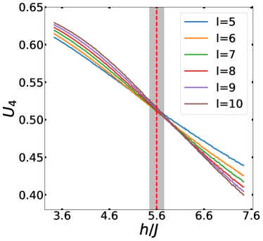
The ground state is found to undergo a ferromagnetic quantum phase transition. The critical disorder strength, averaged over many realizations of the random transverse field, is found by means of a finite-size scaling analysis of the Binder cumulant of the longitudinal magnetization [38, 39]. This analysis is provided in Appendix B. The estimated critical point is .
As in Section III.1, our intent is to obtain the expectation values from a scalable functional written in the form
IV Density functional theory via deep learning
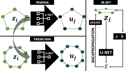
The central task of this study is to train deep neural networks to represent accurate approximations of the unknown universal functional . From here on, the denotes the approximation learned by the neural networks. For both Hamiltonians described in Section III, the universal part can be written as a sum of single-site terms: . Henceforth, the network can be trained to map the array of transverse magnetizations to an equal length array, namely, the set of expectation values , where . Hereafter we describe the network training procedure and the gradient-based optimization used to search for the ground state. A schematic representation of the whole procedure is shown in Fig. 1.
IV.1 Network architecture and training protocol
Special care is taken to implement a scalable neural network, so that it can be applied to different system sizes even without re-training. Some previous studies, which tackled quantum many-body systems within different computational frameworks, have already implemented scalability following various strategies, focusing either on the network architecture and/or on the system descriptors. These strategies include: tiling the systems via parallel networks [40], fixing the output size via global pooling layers [41, 42], including the number of variables as an additional system descriptor [43], or adopting fixed-size system representations [44]. Here, as in Ref. [45], we exploit the linear scaling of the output length with the system size, and we implement scalability by building the network using only convolutional filters. Indeed, convolutional layers are designed to scan their input via fixed-size kernels, but the output size scales with the corresponding input size. Sequences of convolutional layers can be stacked without losing scalability. Specifically, the input layer of our network has neurons corresponding to the -component array . The activations of the neurons in the output layer shall represent the target array . Importantly, the size of the filter kernel , but also the number of convolutional layers , determine the reach of the direct spatial connections accessed by the functionals . Specifically, the output my depend on the input , as long as the modulus of the distance is ( assumed odd). Therefore, as soon as , the DL functionals are highly non-local, and they can easily account for the possible direct coupling between input and output variables corresponding to quite distant spins, already with moderately deep networks. It is known that the type of network architecture affects the performance in simulating quantum systems [46, 47, 48]. After exploring different (convolutional) network models, we choose to adopt an architecture closely inspired by the so-called U-NET [49]. This is built via a sequence of convolutional layers, allowing both standard sequential connections and also skipped connections. The network structure we adopt is visualized in Fig. 2. Each convolutional layer includes channels associated to just as many filters of size . For the first layers the hidden output at the layer is
| (7) |
where . For the next layers, the output of the -th layer in the channel , namely , is computed as:
| (8) |
where is the activation function, and are the weights and biases of the -th layer and .
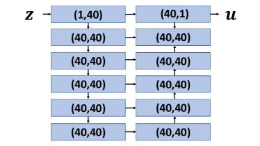
For the results reported in Sections V, layers are used. A further analysis on the effect of different architectural details is reported in the Appendix A. It is worth mentioning that circular padding is adopted in all layers to comply with the periodic boundary condition of the physical system. The network is trained using datasets arranged in the format , where the superscript labels different random realizations of the Hamiltonian. The loss function is the mean squared error , where denotes the number of instances in the training dataset.
The weights and biases are optimized using the ADAM algorithm [50] with batch size , training learning rate , iterated for 3000 epochs. The training datasets include instances, for system sizes in the range . The test datasets include instances, for system sizes . The random fields of the training and testing Hamiltonians are sampled by a uniform distribution in the interval and we consider the critical disorder strength , as well as two values in the paramagnetic and ferromagnetic phases, namely, and , respectively.
IV.2 Gradient-descent minimization
Once the network is trained, the ground-state magnetization profile corresponding to previously unseen Hamiltonian instances can be searched for by minimizing the DL prediction for the energy per spin, which reads:
| (9) |
The exact ground-state energy per spin can then be estimated from the prediction corresponding to the optimal profile , namely . The minimization is performed by iterating gradient-descent updates. To take into account the constraint , a change of variables is performed introducing the angles , such that for . Thus, the update at step is performed as:
| (10) |
where is a small learning rate, while and denote the angles and magnetization profile at step , respectively. A schedule with a fixed learning rate is found to be suitable for all system sizes. Different maximum numbers of gradient-descent steps are considered in the range , depending on the size of the system, with larger sizes requiring more steps to converge to the minimum configuration. The minimization appears not to be affected by local minima; indeed, runs started from different initial random angles converge to the same state. It is also worth pointing out that the gradient-descent procedure turns out not to affected by the instabilities encountered in the use of DL-functionals in continuous-space systems [14, 51, 52, 13, 15]. In that setup, even small errors in the functional derivatives can create nonphysical density profiles, which significantly differ from the ground-state profiles used to train the DL functionals. In that case, the network might provide erroneous predictions that lead to energies even well below the ground state, henceforth violating the variational property held by the exact functional. Several remedial strategies have been adopted, including, e.g, gradient projection [13, 14] or interchannel averaging layers [15]. As shown in Section V, the DL functional implemented here for quantum Ising models do not violate the variational property, in the interesting physical regime, beyond controllable statistical fluctuations.
In Section V, the following figures of merit are used to quantify the performance of our DL-DFT method. The first is the relative energy error of the gradient-descent prediction from the corresponding exact ground-state results . Its disorder average is computed as
| (11) |
where is the number of test Hamiltonian instances. The second is the analogous relative energy error in absolute value . The next figure of merit, , quantifies the accuracy of the magnetization profiles provided by gradient descent. Its disorder average is:
| (12) |
where represents the norm. We also consider the predictions provided by the trained functional when fed with exact ground-state magnetization profiles . Specifically, we focus on the universal contribution , inspecting the relative error compared to the exact ground-state result, namely, . Notice that this metric only accounts for the inaccuracy of the trained functional, thus excluding possible inaccuracies in due to errors occurring in the gradient-descent optimization. It is worth mentioning here that, in Section V.4, also the accuracy of the predictions for the input-output statistical correlations is analyzed, but at a qualitative level.
V Results for gradient-descent optimization
V.1 Accuracy at the quantum critical point
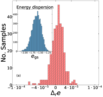
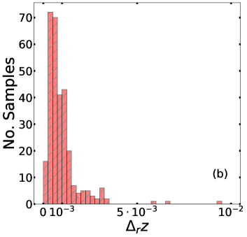
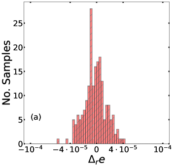
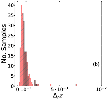
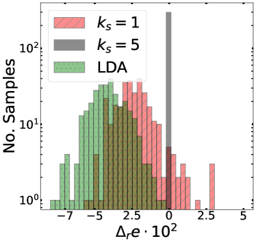
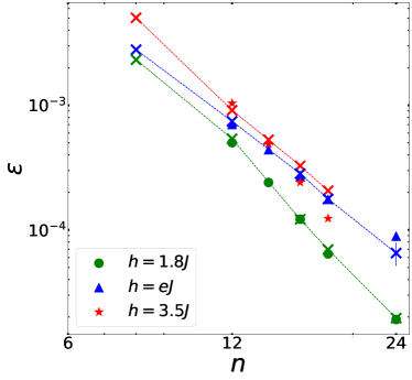
The accuracy of our DL-DFT approach is tested addressing the two random Ising models described in Section III. In this subsection, the gradient descent is performed on the same chain length used for training the network, which is set here at . We first report the performance metrics computed at the quantum critical point, since it is expected to correspond to the worst-case scenario. This issue is further elaborated on in Section V.4. The relative energy discrepancies and the ground-state energy distribution for the 1nn Hamiltonian are shown in Fig (3). The average relative error in absolute value is as small as (the number in parentheses indicates the standard deviation). This is consistent with the residual prediction error computed on exact magnetization profiles. One also notices that negative errors are approximately as likely as the positive ones. This implies that no statistically significant violation of the variational property occurs. The accuracy of the (transverse) magnetization predictions is analyzed in Fig. (3). The average relative error is . A similar accuracy is reached for the 2nn Ising models (see Figs. 4 and 4). Specifically, we obtain and . These performances have been obtained using networks featuring layers, trained on Hamiltonian instances. It is worth stressing that, in fact, the performance can be systematically improved by increasing the network depth and the training dataset size. This is shown in Appendix A.
V.2 Accuracy for varying disorder strength
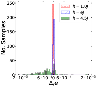
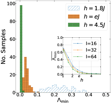
Here we analyze the accuracy of our DL-DFT method for different disorder strengths. The histograms shown in Fig. 5 represent the energy errors after gradient descent for different instances of the 1nn Ising model, at the critical point as well as into the paramagnetic and the ferromagnetic phases. One observes an accuracy degradation at strong disorder, leading also to small violations of the variational property for some Hamiltonian instances. These are due to instabilities in the gradient-descent process 111At large , we also exploit a data augmentation method to partially suppress these instabilities. Each instance in the training dataset is duplicated flipping the sign of , since the target remains unchanged.. Instead, instabilities do not occur at the critical point and in the ferromagnetic phase. To rationalize the degradation in the paramagnetic phase, we consider the conditions required to ensure a bijective map from to (see Section II). At strong disorder , some components of the transverse magnetization might saturate close to . Therefore, changes in might determine numerically imperceptible changes in , essentially leading to an effective breakdown of the bijective property. To quantify this effect, we analyze to what extent the condition defined by Eq. (2), which ensures the bijective property, is fulfilled. Following Ref. [31], we compute the smallest eigenvalue of the matrix (see Eq. (2)), since this allows detecting when the determinant vanishes and, therefore, when the bijective property is not granted. As shown in Fig. 6, vanishingly small eigenvalues occur for large , which is consistent with the accuracy degradation discussed above. While this denotes a possible limitation of the DL-DFT method, it is worth pointing out that the degradation occurs only for very large transverse fields, away from the most relevant regime in the vicinity of the critical point. For large transverse field values, alternative methods, e.g., perturbation theory, are preferable (see, e.g., Refs. [54, 55, 56] and Refs. [57, 58, 59, 60] for applications to Ising models). Furthermore, an alternative formulation of the DL-DFT, namely, one based on the longitudinal magnetization, would be more suitable.
V.3 Comparison with the local density approximation
In the case of continuous-space systems, the most popular approaches to build the universal functional start from the so-called local density approximation (LDA), eventually including semi-local correction terms. The LDA has been adapted to quantum Ising models [19], also considering a nearest-neighbor correction. Within the LDA, the universal functional is computed using the approximation , where denotes the ground-state energy of a homogeneous Ising chain, i.e., one featuring constant transverse fields for and, henceforth, uniform magnetization.
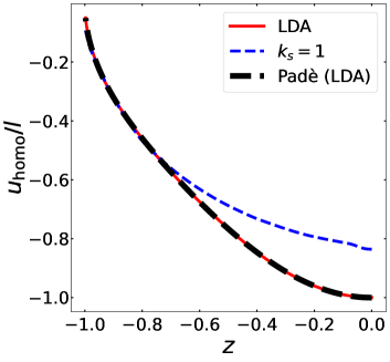
It is interesting to compare the performance of our DL functionals against the plain vanilla LDA. We consider the 1nn Ising chain at the critical point. The LDA functional is determined by performing a best fit on the Jordan-Wigner results for the universal term as a function of the transverse magnetization . The fitting function is a Padè approximant of order . Notice that a purely local functional can be obtained also using our scalable neural networks, simply adopting kernels of size . The comparison is shown in Fig. 7 for the chain length . Notably, even the DL functional is more accurate than the LDA. To rationalize this, we show in Fig. 8 the local function corresponding to the network with , making comparison with the homogeneous approximation . One notices good agreement for , while the two curves substantially differ for larger values of . This implies that, for discrete systems, assuming a homogeneous system featuring a uniform magnetization equal to the local value does not lead to the optimal purely local DFT. In contrast, for continuous-space electronic systems, the equation of state of the homogeneous electron gas is considered to be at least close to the optimal choice [1]. We attribute this discrepancy to the absence of spatial correlations in the random fields, as compared to the external fields , which enter the continuous-space DFT; indeed, these latter functions usually display smooth spatial profiles. Furthermore, in the case of electronic systems, the Hartree term, which accounts for the mean-field direct interactions, is commonly separated from the universal functional. Incidentally, as expected all curves turn out to be essentially flat for , consistently with the symmetry under sign change of the argument . However, we observe that away from our DL functionals do not automatically fulfill this symmetry, even for . This issue can be overcome by performing data augmentation in the training dataset, i.e., randomly adding some configurations with signed-reversed magnetization. In this case, the symmetry is accurately reproduced. For example, for the Hamiltonian at the critical disorder strength at size , the relative prediction error related to the mirror symmetry is as small as .
Importantly, the DL-functional with drastically outperforms the LDA (see Fig. 7). It is worth iterating that, as soon as , the functionals based on deep networks become highly non-local since the spatial extent of the allowed couplings increase layer by layer (see discussion in sub-section IV.1).
To conclude the discussion on local functionals, it is worth further emphasizing that, in Ref. [19], non-local corrections to the LDA have been considered. A functional inspired by so-called generalized gradient approximation (GGA) was implemented to take into account nearest-neighbor effects. This led to a significant improvement in the maximum error, from an error of with the LDA to using the GGA.
V.4 DL-DFT for predicting energies at larger sizes
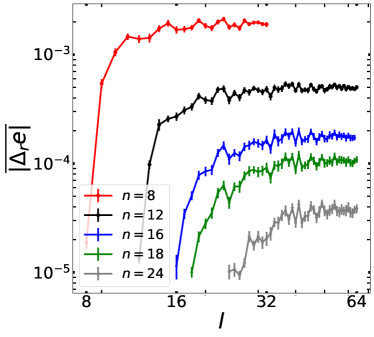
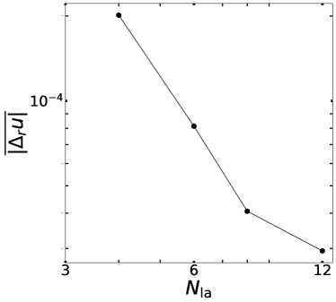
The scalable architecture of our neural networks allows applying the DL functionals to lattices of different lengths. In particular, a functional trained on small lattices can be used to predict the properties of larger systems. However, if the training size is too small, the DL functional might learn spurious finite-size effects, leading to systematic biases in the predictions on the larger test sizes . This effect is investigated hereafter. Notice that, in this subsection, we indicate the training lattice size with , while for the testing size we keep the symbol . In Fig. 9, the average relative error of the gradient descent procedure is analyzed, considering the 1nn Hamiltonian at the critical point. One notices that, after an initial increase, this error metric saturates as the testing systems size increases beyond . Importantly, the asymptotic error systematically decreases as a function of .
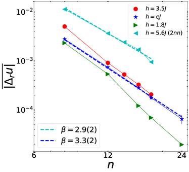
The scaling with of the asymptotic average error is further analyzed in Fig. (10). Only the average prediction accuracy (computed on exact magnetization profiles) is considered, since the gradient descent error generally displays an analogous behavior. The testing system size is , which is suitable to represent the asymptotic large-size regime, for all training sizes we consider. Interestingly, for the system sizes we address, at the critical point the scaling is well described by a power-law fitting function in the form
| (13) |
with the exponent obtained from a best-fit analysis. The 1nn and the 2nn Hamiltonians provide comparable exponents . While this might suggest a possible universal behavior, further models should be analyzed to corroborate this supposition. Notice that, away from the critical points, the error decays even faster, possibly more rapidly than a power-law behavior, but the accessible system sizes do not allow identifying the scaling law. Notice that, as discussed in subsection V.2, when the DL-DFT functional is tested on the size , the inaccuracy amplitude is larger at strong disorder , deep into the paramagnetic phase. Here, we find that, when the test is perform on a size , the scaling with of the inaccuracy is the slowest at the critical point.
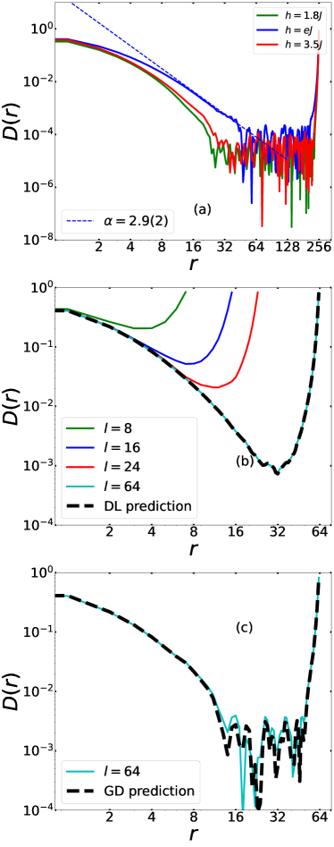
To shed further light on the role of the lattice size on the DL-DFT approach, we investigate the statistical correlations, computed over the disorder realizations, among the inputs and the outputs . Specifically, we compute the (translational invariant) normalized covariance, defined as:
| (14) |
where
| (15) |
with the standard deviation over the disorder realizations. It is worth pointing out that the function does not describe quantum correlations in the ground-state of a specific Hamiltonian, but rather statistical correlations of expectation values in the ensemble of Hamiltonian instances. Here, is computed considering exact ground-state expectation values. Notably, as shown in the panel (a) of Fig. 11, at the critical point and for sufficiently large lattices, the long-distance decay of the correlation function appears to be well described by the power-law , and a best-fit analysis in the region for provides the exponent . The decay is faster away from criticality. These observations suggest a possible connection with the decay of the prediction error . This is further elaborate below. One notices that the long-distance correlations are strongly affected by finite size effects [see panel (b) of Fig. 11]. This might suggest that predictions of DL-functionals trained on small lattices would display strongly biased input-output correlations when tested on larger sizes. Notably, we find this is not the case. This is first demonstrated in panel (b), for the case in which the correlation function is computed using the outputs predicted by networks fed with exact ground-state magnetization profiles. Second, in panel (c), we show the correlations among input and output expectation values obtained from the gradient-descent search of the ground states. Notice that in the latter case only are used, leading to sizable statistical fluctuations compared to the exact ensemble average. Anyway, in both cases the exact correlation function is closely reproduced. In conclusion of this analysis, it is worth pointing out that the statistical correlations discussed here do not imply a direct functional dependence between inputs and (possibly distant) output . Unfortunately, the latter dependence cannot be easily inspected since the ground-state expectation values cannot be independently tuned at will.
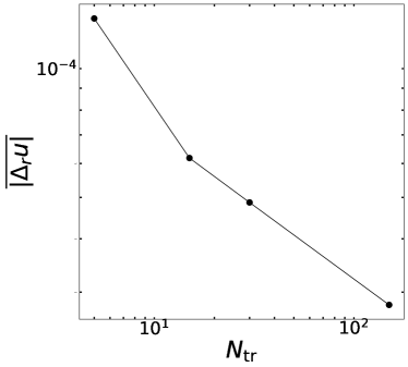
As mentioned above, the scaling of the prediction error appears to relate to the decay of the normalized covariance . This suggests how to build an effective model that explains the observed scaling of with . We assume that the error originates from the discrepancy between the training and the testing correlation functions, denoted here as and . We extrapolate in the interval with and even numbers, by using a best fit with a stretched exponential ( are the fitting parameters), performed in the interval for and for . The prediction error on a site is supposed to be due to contributions from all correlation discrepancies outside the training window . The contribution for the distance is represented as a Gaussian random variable of zero mean and standard deviation , The total error results from the contributions outside the training window
| (16) |
where the two sums represent the contribution of the cutoff windows and , respectively. The final estimate of the prediction error is
| (17) |
In Fig. (12), the scaling of the estimated error is compared with the actual prediction errors , for the testing system size , three disorder strengths , and training sizes . Notice that the goal is only to compare the scaling with , and, in fact, is scaled with an appropriate prefactor. Interestingly, this heuristic model is able to accurately capture the scaling of the prediction error with the training size for and . For the estimation predicts a slightly faster decay in the error compared to the actual scaling. This discrepancy can be attributed to the increased difficulty in accurately reproducing a bijective map from to in the strong disorder regime, as discussed in Section V.2. Indeed, this effect is not accounted for in this model.
VI Conclusions
We have shown that an accurate DFT approach for disordered quantum Ising chains can be implemented using scalable neural networks. These networks accurately map the transverse magnetization profile to the ground-state energy, and they allow finding the energy and magnetization of previously unseen realization of the random fields via a computationally efficient gradient-descent minimization of the predicted energy. Notably, the scalable architecture allows predicting the properties of systems much larger than those used to train the network. This finding indicates a promising strategy to extend the reach of existing computational techniques which are accurate but limited to relatively small system sizes. Indeed, the prediction error in the thermodynamics limit rapidly decreases as a function of the size used for training; specifically, the error approximately scales as in the worst case scenario, namely, at the quantum critical point, or even faster away from criticality. Further investigations, which we leave for future studies, are due to establish the possible universality of the critical scaling. Our analysis allowed us to shed light on the non-local character of the energy functional. Our DL-DFT approach systematically outperforms the purely local LDA and, thanks to increased kernel sizes and/or network depths, is able to capture long-range input-output functional dependencies. It was also shown that, even when trained on relatively small system sizes, the DL functionals allow reconstructing the statistical correlations among input and output expectation values corresponding to very distant sites. Finally, a heuristic model that describes the scaling of the prediction accuracy with the training size has been provided. Future studies could also address higher dimensional systems or extend the DL approach to time-dependent DFT for quantum spin models [61]. The resilience of DL functional to noisy training datasets should also be explored [41, 62], as this could pave the way to learning DFTs from experimental measurements.
Acknowledgments
E.C. acknowledges hospitality in the QOQMS group led by A. Daley at the University of Strathclyde. E.C. also acknowledges R. Connor from the QOQMS group and G. Scriva from the University of Camerino, for the interesting discussions and suggestions. S.P. and R.F. acknowledge support from the PNRR MUR project PE0000023-NQSTI. S.P also acknowledges support from the Italian Ministry of University and Research under the PRIN2017 project CEnTraL 20172H2SC4, and from the CINECA award IscrC-NEMCAQS (2023), for the availability of high performance computing resources and support, as well as from PRACE, for awarding access to the Fenix Infrastructure resources at Cineca, which are partially funded by the European Union’s Horizon 2020 research and innovation program through the ICEI project under the Grant Agreement No. 800858.
Appendix A Systematic improvement of the prediction accuracy
In Section V, the accuracy of our DL functionals has been analyzed considering a fixed network structure and one training protocol. The error metrics were remarkably small. More important, perhaps, is that the error can be systematically controlled by increasing the network depth and/or the size of the training dataset. This is shown in Figs. 13 and 14. The 1nn Hamiltonian at the critical point is addressed. Only the prediction accuracy is considered, since this metric also determines the error in the subsequent gradient-descent procedure. Specifically, we show that the prediction error rapidly decreases when the number of training instances increases, and also when the depth of the network is augmented.
Appendix B Ferromagnetic phase transition in the next-nearest neighbor Ising chain
To determine the critical point of the ferromagnetic quantum phase transition in the Ising model, we perform a finite-size scaling analysis of the so-called Binder cumulant [38], defined as:
| (18) |
This is computed via exact diagonalization, as a function of the disorder strengths and for different chain lengths . The disorder average is performed over instances of the Hamiltonian. The results are shown in Fig. 15. The crossing of the datasets corresponding to different chain lengths denotes the critical point. This allows us to approximately estimate the critical disorder strength to be .
References
- Burke [2012] K. Burke, Perspective on density functional theory, J. Chem. Phys. 136, 150901 (2012).
- Cohen et al. [2012] A. J. Cohen, P. Mori-Sánchez, and W. Yang, Challenges for density functional theory, Chem. Rev. 112, 289 (2012).
- Dunjko and Briegel [2018] V. Dunjko and H. J. Briegel, Machine learning & artificial intelligence in the quantum domain: A review of recent progress, Rep. Prog. Phys. 81, 074001 (2018).
- Carleo et al. [2019] G. Carleo, I. Cirac, K. Cranmer, L. Daudet, M. Schuld, N. Tishby, L. Vogt-Maranto, and L. Zdeborová, Machine learning and the physical sciences, Rev. Mod. Phys. 91, 045002 (2019).
- Carrasquilla [2020] J. Carrasquilla, Machine learning for quantum matter, Adv. Phys.-X 5, 1797528 (2020).
- Kulik et al. [2022] H. J. Kulik, T. Hammerschmidt, J. Schmidt, S. Botti, M. A. L. Marques, M. Boley, M. Scheffler, M. Todorović, P. Rinke, C. Oses, A. Smolyanyuk, S. Curtarolo, A. Tkatchenko, A. P. Bartók, S. Manzhos, M. Ihara, T. Carrington, J. Behler, O. Isayev, M. Veit, A. Grisafi, J. Nigam, M. Ceriotti, K. T. Schütt, J. Westermayr, M. Gastegger, R. J. Maurer, B. Kalita, K. Burke, R. Nagai, R. Akashi, O. Sugino, J. Hermann, F. Noé, S. Pilati, C. Draxl, M. Kuban, S. Rigamonti, M. Scheidgen, M. Esters, D. Hicks, C. Toher, P. V. Balachandran, I. Tamblyn, S. Whitelam, C. Bellinger, and L. M. Ghiringhelli, Roadmap on machine learning in electronic structure, Electron. struct. 4, 023004 (2022).
- Brockherde et al. [2017] F. Brockherde, L. Vogt, L. Li, M. E. Tuckerman, K. Burke, and K.-R. Müller, Bypassing the Kohn-Sham equations with machine learning, Nat. Commun. 8, 872 (2017).
- Li et al. [2021] L. Li, S. Hoyer, R. Pederson, R. Sun, E. D. Cubuk, P. Riley, and K. Burke, Kohn-sham equations as regularizer: Building prior knowledge into machine-learned physics, Phys. Rev. Lett. 126, 036401 (2021).
- Li et al. [2016a] L. Li, T. E. Baker, S. R. White, and K. Burke, Pure density functional for strong correlation and the thermodynamic limit from machine learning, Phys. Rev. B 94, 245129 (2016a).
- Kirkpatrick et al. [2021] J. Kirkpatrick, B. McMorrow, D. H. P. Turban, A. L. Gaunt, J. S. Spencer, A. G. D. G. Matthews, A. Obika, L. Thiry, M. Fortunato, D. Pfau, L. R. Castellanos, S. Petersen, A. W. R. Nelson, P. Kohli, P. Mori-Sánchez, D. Hassabis, and A. J. Cohen, Pushing the frontiers of density functionals by solving the fractional electron problem, Science 374, 1385 (2021).
- Nelson et al. [2019] J. Nelson, R. Tiwari, and S. Sanvito, Machine learning density functional theory for the Hubbard model, Phys. Rev. B 99, 075132 (2019).
- Ryczko et al. [2022] K. Ryczko, S. J. Wetzel, R. G. Melko, and I. Tamblyn, Toward orbital-free density functional theory with small data sets and deep learning, J. Chem. Theory Comput. 18, 1122–1128 (2022).
- Meyer et al. [2020] R. Meyer, M. Weichselbaum, and A. W. Hauser, Machine learning approaches toward orbital-free density functional theory: Simultaneous training on the kinetic energy density functional and its functional derivative, J. Chem. Theory Comput. 16, 5685 (2020).
- Snyder et al. [2015] J. C. Snyder, M. Rupp, K.-R. Müller, and K. Burke, Nonlinear gradient denoising: Finding accurate extrema from inaccurate functional derivatives, Int. J. Quantum Chem. 115, 1102 (2015).
- Costa et al. [2022] E. Costa, G. Scriva, R. Fazio, and S. Pilati, Deep-learning density functionals for gradient descent optimization, Phys. Rev. E 106, 045309 (2022).
- Coe [2019] J. P. Coe, Lattice density-functional theory for quantum chemistry, Phys. Rev. B 99, 165118 (2019).
- Penz and van Leeuwen [2021] M. Penz and R. van Leeuwen, Density-functional theory on graphs, J. Chem. Phys. 155, 244111 (2021), https://doi.org/10.1063/5.0074249 .
- Líbero and Capelle [2003] V. L. Líbero and K. Capelle, Spin-distribution functionals and correlation energy of the heisenberg model, Phys. Rev. B 68, 024423 (2003).
- Mao et al. [2021] J. Mao, H. Tang, W. Duan, and Z. Liu, Testing density functional theory in a quantum Ising chain, Phys. Rev. B 104, 155145 (2021).
- Scholl et al. [2021] P. Scholl, M. Schuler, H. J. Williams, A. A. Eberharter, D. Barredo, K.-N. Schymik, V. Lienhard, L.-P. Henry, T. C. Lang, T. Lahaye, A. M. Läuchli, and A. Browaeys, Quantum simulation of 2d antiferromagnets with hundreds of rydberg atoms, Nature 595, 233 (2021).
- Omran et al. [2019] A. Omran, H. Levine, A. Keesling, G. Semeghini, T. T. Wang, S. Ebadi, H. Bernien, A. S. Zibrov, H. Pichler, S. Choi, J. Cui, M. Rossignolo, P. Rembold, S. Montangero, T. Calarco, M. Endres, M. Greiner, V. Vuletić, and M. D. Lukin, Generation and manipulation of schrödinger cat states in rydberg atom arrays, Science 365, 570 (2019), https://www.science.org/doi/pdf/10.1126/science.aax9743 .
- Smith et al. [2016] J. Smith, A. Lee, P. Richerme, B. Neyenhuis, P. W. Hess, P. Hauke, M. Heyl, D. A. Huse, and C. Monroe, Many-body localization in a quantum simulator with programmable random disorder, Nat. Phys. 12, 907 (2016).
- Morong et al. [2021] W. Morong, F. Liu, P. Becker, K. S. Collins, L. Feng, A. Kyprianidis, G. Pagano, T. You, A. V. Gorshkov, and C. Monroe, Observation of stark many-body localization without disorder, Nature 599, 393 (2021).
- Boixo et al. [2014] S. Boixo, T. F. Rønnow, S. V. Isakov, Z. Wang, D. Wecker, D. A. Lidar, J. M. Martinis, and M. Troyer, Evidence for quantum annealing with more than one hundred qubits, Nat. Phys. 10, 218 (2014).
- Pitsios et al. [2017] I. Pitsios, L. Banchi, A. S. Rab, M. Bentivegna, D. Caprara, A. Crespi, N. Spagnolo, S. Bose, P. Mataloni, R. Osellame, et al., Photonic simulation of entanglement growth and engineering after a spin chain quench, Nat. Commun. 8, 1569 (2017).
- Murmann et al. [2015] S. Murmann, F. Deuretzbacher, G. Zürn, J. Bjerlin, S. M. Reimann, L. Santos, T. Lompe, and S. Jochim, Antiferromagnetic heisenberg spin chain of a few cold atoms in a one-dimensional trap, Phys. Rev. Lett. 115, 215301 (2015).
- Jepsen et al. [2020] P. N. Jepsen, J. Amato-Grill, I. Dimitrova, W. W. Ho, E. Demler, and W. Ketterle, Spin transport in a tunable heisenberg model realized with ultracold atoms, Nature 588, 403 (2020).
- Hohenberg and Kohn [1964] P. Hohenberg and W. Kohn, Inhomogeneous electron gas, Phys. Rev. 136, B864 (1964).
- Levy [1979] M. Levy, Universal variational functionals of electron densities, first-order density matrices, and natural spin-orbitals and solution of the -representability problem, Proc. Natl. Acad. Sci. U.S.A. 76, 6062 (1979).
- Lieb [1983] E. Lieb, Density functionals for Coulomb systems, Int. J. Quantum Chem. 24, 243 (1983).
- Xu et al. [2022] L. Xu, J. Mao, X. Gao, and Z. Liu, Extensibility of hohenberg–kohn theorem to general quantum systems, Adv. Quantum Technol. 5, 2200041 (2022), https://onlinelibrary.wiley.com/doi/pdf/10.1002/qute.202200041 .
- Lieb et al. [1961] E. Lieb, T. Schultz, and D. Mattis, Two soluble models of an antiferromagnetic chain, Ann. Phys. 16, 407 (1961).
- Mbeng et al. [2020] G. B. Mbeng, A. Russomanno, and G. E. Santoro, The quantum Ising chain for beginners (2020), arXiv:2009.09208 [quant-ph] .
- Pfeuty [1979] P. Pfeuty, An exact result for the 1d random Ising model in a transverse field, Phys. Lett. A 72, 245 (1979).
- Young and Rieger [1996] A. P. Young and H. Rieger, Numerical study of the random transverse-field Ising spin chain, Phys. Rev. B 53, 8486 (1996).
- Weinberg and Bukov [2017] P. Weinberg and M. Bukov, QuSpin: a Python package for dynamics and exact diagonalisation of quantum many body systems part I: spin chains, SciPost Phys. 2, 003 (2017).
- Fishman et al. [2022] M. Fishman, S. R. White, and E. M. Stoudenmire, The ITensor Software Library for Tensor Network Calculations, SciPost Phys. Codebases , 4 (2022).
- Binder [1981] K. Binder, Finite size scaling analysis of Ising model block distribution functions, Zeitschrift für Physik B Condensed Matter 43, 119 (1981).
- Kalinowski et al. [2022] M. Kalinowski, R. Samajdar, R. G. Melko, M. D. Lukin, S. Sachdev, and S. Choi, Bulk and boundary quantum phase transitions in a square rydberg atom array, Phys. Rev. B 105, 174417 (2022).
- Mills et al. [2019] K. Mills, K. Ryczko, I. Luchak, A. Domurad, C. Beeler, and I. Tamblyn, Extensive deep neural networks for transferring small scale learning to large scale systems, Chem. Sci. 10, 4129 (2019).
- Saraceni et al. [2020] N. Saraceni, S. Cantori, and S. Pilati, Scalable neural networks for the efficient learning of disordered quantum systems, Phys. Rev. E 102, 033301 (2020).
- Cantori et al. [2023] S. Cantori, D. Vitali, and S. Pilati, Supervised learning of random quantum circuits via scalable neural networks, Quantum Sci. Technol. 8, 025022 (2023).
- Mujal et al. [2021] P. Mujal, Àlex Martínez Miguel, A. Polls, B. Juliá-Díaz, and S. Pilati, Supervised learning of few dirty bosons with variable particle number, SciPost Phys. 10, 73 (2021).
- Jung et al. [2020] H. Jung, S. Stocker, C. Kunkel, H. Oberhofer, B. Han, K. Reuter, and J. T. Margraf, Size-extensive molecular machine learning with global representations, Chem Systems Chem 2, e1900052 (2020).
- Blania et al. [2022] A. Blania, S. Herbig, F. Dechent, E. van Nieuwenburg, and F. Marquardt, Deep learning of spatial densities in inhomogeneous correlated quantum systems (2022), arXiv:2211.09050 [quant-ph] .
- Hermann et al. [2020] J. Hermann, Z. Schätzle, and F. Noé, Deep-neural-network solution of the electronic Schrödinger equation, Nat. Chem. 12, 891 (2020).
- Pilati and Pieri [2020] S. Pilati and P. Pieri, Simulating disordered quantum Ising chains via dense and sparse restricted Boltzmann machines, Phys. Rev. E 101, 063308 (2020).
- Lou et al. [2023] W. T. Lou, H. Sutterud, G. Cassella, W. M. C. Foulkes, J. Knolle, D. Pfau, and J. S. Spencer, Neural wave functions for superfluids (2023), arXiv:2305.06989 [cond-mat.quant-gas] .
- Ronneberger et al. [2015] O. Ronneberger, P. Fischer, and T. Brox, U-net: Convolutional networks for biomedical image segmentation (2015), arXiv:1505.04597 [cs.CV] .
- Kingma and Ba [2014] D. P. Kingma and J. Ba, Adam: A method for stochastic optimization, arXiv:1412.6980 (2014).
- Snyder et al. [2012] J. C. Snyder, M. Rupp, K. Hansen, K.-R. Müller, and K. Burke, Finding density functionals with machine learning, Phys. Rev. Lett. 108, 253002 (2012).
- Li et al. [2016b] L. Li, J. C. Snyder, I. M. Pelaschier, J. Huang, U.-N. Niranjan, P. Duncan, M. Rupp, K.-R. Müller, and K. Burke, Understanding machine-learned density functionals, Int. J. Quantum Chem. 116, 819 (2016b).
- Note [1] At large , we also exploit a data augmentation method to partially suppress these instabilities. Each instance in the training dataset is duplicated flipping the sign of , since the target remains unchanged.
- Brueckner [1955] K. A. Brueckner, Many-body problem for strongly interacting particles. ii. linked cluster expansion, Phys. Rev. 100, 36 (1955).
- Coester and Schmidt [2015] K. Coester and K. P. Schmidt, Optimizing linked-cluster expansions by white graphs, Phys. Rev. E 92, 022118 (2015).
- Coester et al. [2016] K. Coester, D. G. Joshi, M. Vojta, and K. P. Schmidt, Linked-cluster expansions for quantum magnets on the hypercubic lattice, Phys. Rev. B 94, 125109 (2016).
- Moessner and Sondhi [2001] R. Moessner and S. L. Sondhi, Ising models of quantum frustration, Phys. Rev. B 63, 224401 (2001).
- Chakrabarti et al. [2008] B. K. Chakrabarti, A. Dutta, and P. Sen, Quantum Ising phases and transitions in transverse Ising models, Vol. 41 (Springer Science & Business Media, 2008).
- Mossi et al. [2017] G. Mossi, T. Parolini, S. Pilati, and A. Scardicchio, On the quantum spin glass transition on the Bethe lattice, J. Stat. Mech.: Theory Exp. 2017 (1), 013102.
- Dusuel et al. [2010] S. Dusuel, M. Kamfor, K. P. Schmidt, R. Thomale, and J. Vidal, Bound states in two-dimensional spin systems near the Ising limit: A quantum finite-lattice study, Phys. Rev. B 81, 064412 (2010).
- Tempel and Aspuru-Guzik [2012] D. G. Tempel and A. Aspuru-Guzik, Quantum computing without wavefunctions: Time-dependent density functional theory for universal quantum computation, Sci. Rep. 2, 391 (2012).
- Pilati and Pieri [2019] S. Pilati and P. Pieri, Supervised machine learning of ultracold atoms with speckle disorder, Sci. Rep. 9, 10.1038/s41598-019-42125-w (2019).