SAMScore: A Semantic Structural Similarity Metric for Image Translation Evaluation

Abstract

Image translation has wide applications, such as style transfer and modality conversion, usually aiming to generate images having both high degrees of realism and faithfulness. These problems remain difficult, especially when it is important to preserve semantic structures. Traditional image-level similarity metrics are of limited use, since the semantics of an image are high-level, and not strongly governed by pixel-wise faithfulness to an original image. Towards filling this gap, we introduce SAMScore, a generic semantic structural similarity metric for evaluating the faithfulness of image translation models. SAMScore is based on the recent high-performance Segment Anything Model (SAM), which can perform semantic similarity comparisons with standout accuracy. We applied SAMScore on 19 image translation tasks, and found that it is able to outperform all other competitive metrics on all of the tasks. We envision that SAMScore will prove to be a valuable tool that will help to drive the vibrant field of image translation, by allowing for more precise evaluations of new and evolving translation models. The code is available at https://github.com/Kent0n-Li/SAMScore.

I Introduction

Image translation, including tasks such as style transfer and modality conversion, has been a highly active research area in computer vision and deep learning [1, 2, 3, 4, 5, 6]. Image translation tasks aim to generate images in a target domain while ensuring the adequate preservation of semantic structural information intrinsic to the source image [7, 8, 9]. The diverse applications of image translation, ranging from medical image processing [6] to autonomous driving [10], have fueled significant interests in this field. Across these many domains, one of the primary challenges in achieving high-quality image translation is the preservation of semantic structure in the generated images (faithfulness) [11, 12, 13]. However, there is a lack of accepted or effective methods for evaluating the ability of image translation to produce results that exhibit satisfactory semantic structure. We believe that addressing this missing need will prove to be an essential ingredient for advancing the field of image translation.

Conventional image-level similarity metrics, such as the L2 norm, Peak Signal-to-Noise Ratio (PSNR), and Structural Similarity Index (SSIM) [14], despite their ability to measure image similarity, are inadequate for this purpose. Their deficiency lies in their inability to incorporate high-level semantic understanding into their measurements in a manner that does not require pixel-to-pixel similarity [15]. This flaw becomes evident when considering the measurement of the translation from a black cat to a white cat using any of the aforementioned similarity models. Likewise, the Learned Perceptual Image Patch Similarity (LPIPS) metric [11], which does utilize high-level information, falls short as well since it is not designed with the purpose of evaluating semantic structures, instead measuring only perceived similarities between images in the presence of common distortions, which is still too limited. FCNScore [12, 16, 1], which employs fully convolutional networks to conduct image semantic segmentation and indirectly access the structural similarity via accurate segmentation, has its own set of issues. These include the necessity of labels to train segmentation networks, a lack of granularity of structure evaluation, and the domain gap between the generated images and the target images.

The recent emergence of the Segment Anything Model (SAM) [17], which is an exceptionally powerful deep segmentation model, provides a new way to address these issues. SAM possesses a strong zero-shot generalization capability and scalability to other domains [18] and is able to extract highly generic semantic structural information. We exploit this timely advancement to develop a new image similarity metric that we call SAMScore, which leverages SAM to evaluate semantic structural similarities between original source images and generatively-translated versions of them.

Our contributions are summarized as follows:

• We propose a universal metric for assessing semantic structural similarity, which addresses the current lack of any general metric for evaluating the semantic faithfulness of image translation tasks.

• We show that SAMScore outperforms existing similarity metrics in evaluating semantic structural similarity across 19 image translation tasks, demonstrating superior effectiveness and robustness.

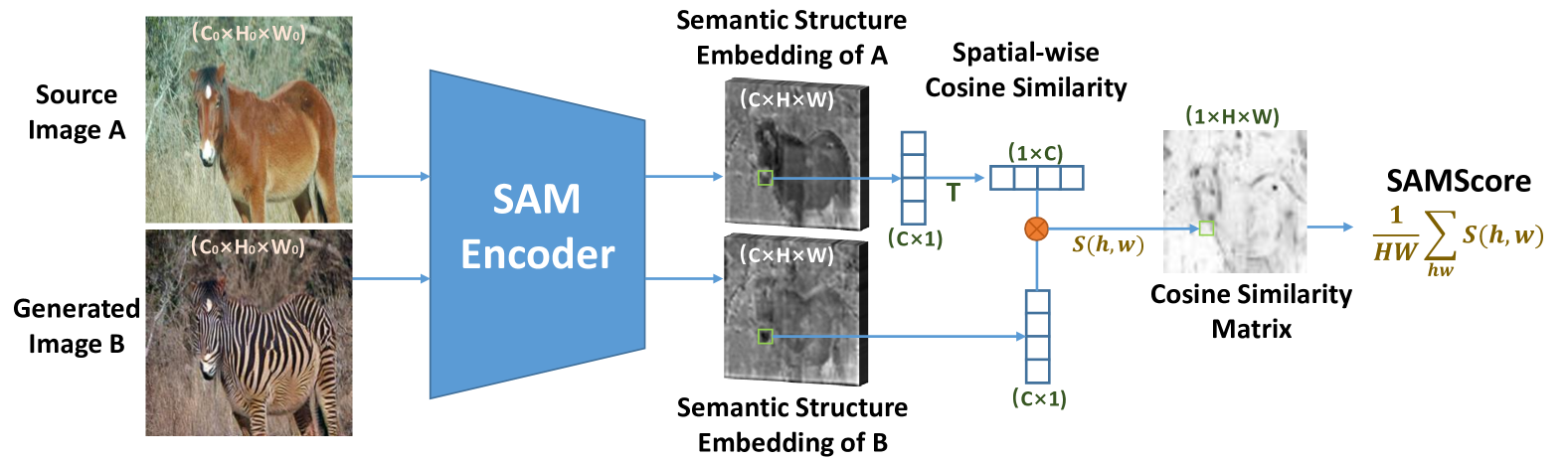
Figure 1: Overview of SAMScore. Source and generated images are separately input to the SAM encoder to obtain embeddings of the semantic structures, then a spatial cosine similarity score is calculated, yielding the final SAMScore.

II Related Work

The primary goal of image translation is to map and transform images between different domains. Although various techniques have been developed, their core objective remains the same, which is to achieve realistic and faithful image translations. Faithfulness here refers to the preservation of the semantic structure information from the source image. Previous methods for evaluating faithfulness similarity include L2 (Euclidean distance or MSE), PSNR (Peak Signal-to-Noise Ratio), SSIM (Structural Similarity Index) [14], LPIPS (Learned Perceptual Image Patch Similarity) [11], and FCNScore (semantic segmentation accuracy by Fully Convolutional Network) [12, 16, 1].

L2 is a widely used metric that compares images pixel by pixel. Despite being simple and easy to calculate, L2 has limitations that make it unsuitable for most image translation tasks. For instance, it is sensitive to image intensity range shifts, causing significant differences even if the content/structure of the images remains similar.

PSNR is a common metric often used to assess image compression. It is equivalent to L2, and so also falls short in assessing semantic structural similarity.

SSIM captures perceptual similarity more accurately than L2/PSNR by accounting for perceptual masking and local structure [14]. However, SSIM lacks the ability to capture the semantic content of images.

LPIPS is a deep learning-based metric that measures the distance or difference between image patches, by computing the similarity between the activations of two images output by a neural network [11]. While LPIPS accurately predicts perceptual similarity between images, it does not capture semantic structural similarity.

FCNScore is an image translation evaluation metric based on the segmentation accuracy [12, 16, 1]. This metric requires training a fully connected segmentation network applied on target domain images when conducting a specific segmentation task. It also requires segmentation labels for the same task to be available on the source domain images. Semantic structure similarity is by measuring the accuracy and IoU of the segmentation results of the source images and the generated images. However, FCNScore has a high cost of targeted training, and structural granularity measurement is limited by the granularity of the segmentation labels.

Evaluating the semantic faithfulness of image translation has been a challenging task, with previous studies adopting different approaches. Some, such as GcGAN [19] and CUT [20], employ the FCNScore metric to assess semantic structural similarity. MUNIT [21] and StarGANv2 [22] use human evaluations obtained via Amazon Mechanical Turk (AMT) [23], but this introduces significant subjectivity and scalability challenges. CycleGAN [16] and pix2pix [1] combine FCNScore and AMT to leverage the strengths of both metrics, but this method still has intrinsic limitations. In recent diffusion model-based methods, the datasets used lack available segmentation labels, hence L2, PSNR, SSIM, and LPIPS metrics are used instead of FCNScore. BBDM [24] uses LPIPS for evaluation, SDEdit [25] applies L2 and LPIPS, CycleDiffusion [26] employs PSNR and SSIM, and EGSDE [27] uses L2 along with PSNR and SSIM. Although these models effectively measure differences, they do not specifically evaluate semantic structural similarity.

III SAMScore

To address the limitations of the existing similarity metrics described in the previous section, we introduce SAMScore, which uses the encoder portion of the foundational Segment Anything Model (SAM) to obtain rich semantic structural embeddings of both source and generated images to be compared, then measures semantic structural similarity by calculating the cosine similarity, as shown in Figure 1.

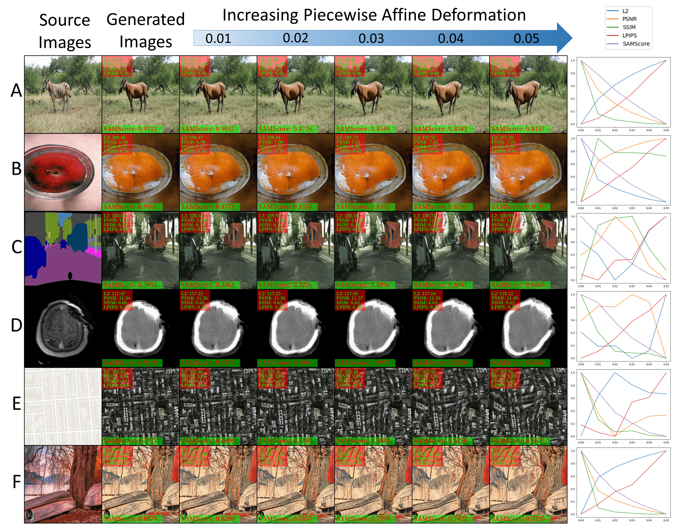
Figure 2: Similarity scores between the original images and CycleGAN-generated images with varying degrees of deformation. (A) horse to zebra, (B) orange to apple, (C) cityscapes (label to photo), (D) head (MR to CT), (E) photo to Ukiyoe, and (F) photo to Monet. Column 2 shows the results without additional distortion. Given the varying scales of the metrics, we standardized each metric to [0,1] before generating the line chart.

III-A SAM Encoder

We first map the source and the translated (generated) images into high-level image embedding spaces that are rich in semantic structural information. We deploy the SAM Encoder $\mathcal{E}(\cdot)$ to extract semantic embeddings of both the source image and the translated image, denoted as $X_{E}$ and $Y_{E}$, respectively. The large and extensive segmentation data that was used to train the encoder in SAM imparts it with the capability to extract semantic information from “any” images, viz., it is extremely generalizable. Given its ability to represent images as compact semantic embedding vectors, SAM avoids the influence of low-level information discrepancies of local color/texture between two compared images. Given a source image $X_{0}\in\mathbb{R}^{C_{0}\times H_{0}\times W_{0}}$ and a generated image $Y_{0}\in\mathbb{R}^{C_{0}\times H_{0}\times W_{0}}$, let:

$$X_{E}=\mathcal{E}(X_{0}),~{}Y_{E}=\mathcal{E}(Y_{0}),$$ (1)

where $X_{E},Y_{E}\in\mathbb{R}^{C\times H\times W}$ are the respective embeddings, and $C$, $H$, and $W$ are the number of channels, the height, and the width of the SAM encoder output embedding. In the standard SAM encoder, $C$ is 256, and the $H$ and $W$ are 1/16 of the input image’s height $H_{0}$ and width $W_{0}$, respectively.

III-B Similarity Metrics

After obtaining the vectors of the embedded semantic structure of the source and the translated images, we measure their similarity by the cosine similarity, which is a simple but effective target to compare the similarity of two vectors. Cosine similarity measures the cosine of the angle between two vectors, taking into account the direction of the vectors rather than their size. This provides robustness when comparing tensor features, and in the presence of small amounts of noise. Since semantic structural information is spatial, we calculate the similarity of the two embeddings at the spatial level. The cosine similarity between the two vectors in Equation 1 at spatial position $(h,w)$ is:

$$S(X_{E}^{hw},Y_{E}^{hw})=\frac{(X_{E}^{hw})^{\top}Y_{E}^{hw}}{||X_{E}^{hw}||_{2}~{}||Y_{E}^{hw}||_{2}}.$$ (2)

The overall SAMScore between the source image and the generated image is then:

$$SAMScore(X_{E},Y_{E}) =\frac{1}{HW}\sum_{h,w}S(X_{E}^{hw},Y_{E}^{hw})$$ (3)

$$=\frac{1}{HW}\sum_{h,w}\frac{(\mathcal{E}^{hw}(X_{0}))^{\top}\mathcal{E}^{hw}(Y_{0})}{||\mathcal{E}^{hw}(X_{0})||_{2}~{}||\mathcal{E}^{hw}(Y_{0})||_{2}}.$$

TABLE I: Absolute correlation coefficients of image similarity metrics on a variety of image translation tasks, where the images have been corrupted by varying amounts of affine geometric distortions. Since deformation changes image semantic structural information, a higher correlation is better as it shows a metric can better capture the semantic differences between the source and translated images.

Task	L2	PSNR	SSIM	LPIPS	SAMScore
apple to orange	0.7817	0.7810	0.8223	0.8871	0.9116
orange to apple	0.7967	0.7958	0.8390	0.9134	0.9315
cityscapes (label to photo)	0.4577	0.4570	0.4914	0.7801	0.9136
cityscapes (photo to label)	0.4635	0.4633	0.4824	0.6150	0.7892
facades (label to photo)	0.7460	0.7457	0.6943	0.7740	0.9549
facades (photo to label)	0.7739	0.7734	0.7087	0.7095	0.9479
head (MR to CT)	0.5279	0.5278	0.7134	0.7655	0.7734
head (CT to MR)	0.7281	0.7304	0.7798	0.8208	0.8553
horse to zebra	0.9276	0.9183	0.8190	0.9169	0.9497
zebra to horse	0.9337	0.9235	0.8334	0.9446	0.9564
Monet to photo	0.8548	0.8377	0.7701	0.9395	0.9444
photo to Monet	0.9088	0.8992	0.7895	0.9386	0.9487
aerial photograph to map	0.7275	0.7275	0.7827	0.7997	0.9326
map to aerial photograph	0.5481	0.5483	0.7321	0.7984	0.9317
photo to Cezanne	0.9240	0.9155	0.8178	0.9161	0.9338
photo to Ukiyoe	0.8963	0.8917	0.7798	0.9148	0.9261
photo to Vangogh	0.9109	0.9009	0.7745	0.9137	0.9273
Yosemite (summer to winter)	0.9183	0.9201	0.6889	0.9372	0.9545
Yosemite (winter to summer)	0.9205	0.9224	0.7297	0.9399	0.9488

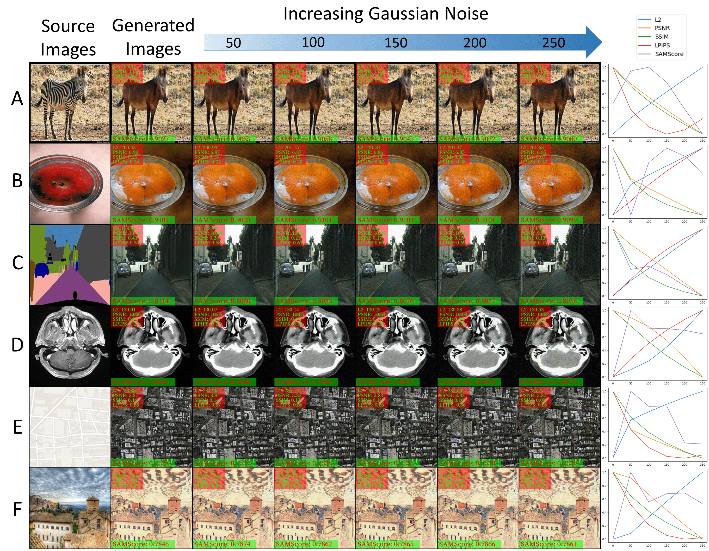
Figure 3: Similarity scores between the original images and CycleGAN-generated images with varying degrees of Gaussian noise corruption. (A) horse to zebra, (B) orange to apple, (C) cityscapes (label to photo), (D) head (MR to CT), (E) photo to Ukiyoe, and (F) photo to Monet. Column 2 shows results without additional distortion. Given the varying scales of the metrics, we standardized each metric to [0,1] before generating the line chart.

TABLE II: Absolute correlation coefficients of image similarity metrics on a variety of image translation tasks, where the images have been corrupted by varying degrees of Gaussian Noises. Since Gaussian noise does not significantly change image semantic structural information, unless it is very heavy, a lower correlation is better as it shows the metric is less susceptible to random noise-induced intensity variations between the source and the translated images.

Task	L2	PSNR	SSIM	LPIPS	SAMScore
apple to orange	0.8180	0.8179	0.9200	0.9435	0.6538
orange to apple	0.8511	0.8511	0.9220	0.9506	0.6953
cityscapes (label to photo)	0.9950	0.9948	0.9269	0.9925	0.3881
cityscapes (photo to label)	0.9845	0.9847	0.9255	0.9855	0.4935
facades (label to photo)	0.9392	0.9392	0.9444	0.9300	0.7025
facades (photo to label)	0.9693	0.9698	0.9523	0.7487	0.7603
head (MR to CT)	0.7873	0.7852	0.9227	0.9777	0.8248
head (CT to MR)	0.9737	0.9731	0.9133	0.9878	0.5703
horse to zebra	0.9975	0.9963	0.9586	0.8996	0.7928
zebra to horse	0.9985	0.9980	0.9638	0.9476	0.7876
Monet to photo	0.9879	0.9853	0.9609	0.7952	0.8324
photo to Monet	0.9902	0.9903	0.9596	0.9669	0.7711
aerial photograph to map	0.8792	0.8795	0.9583	0.9814	0.8697
map to aerial photograph	0.8907	0.8904	0.9602	0.7700	0.5797
photo to Cezanne	0.9983	0.9976	0.9575	0.8436	0.7012
photo to Ukiyoe	0.9851	0.9853	0.9595	0.8385	0.6482
photo to Vangogh	0.9974	0.9973	0.9722	0.8345	0.6318
Yosemite (summer to winter)	0.9985	0.9982	0.9364	0.9317	0.8234
Yosemite (winter to summer)	0.9975	0.9969	0.9405	0.9538	0.8333

TABLE III: Absolute correlation coefficients of image similarity measured by FCNScore and SAMScore on the cityscapes (label to photo) task, where the translated images have been distorted by varying degrees of affine geometric deformations and Gaussian Noises.

Image Transformation	per-pixel ACC	class IoU	SAMScore
Deformation	0.6693	0.8353	0.9136
Gaussian Noise	0.7119	0.7980	0.3881

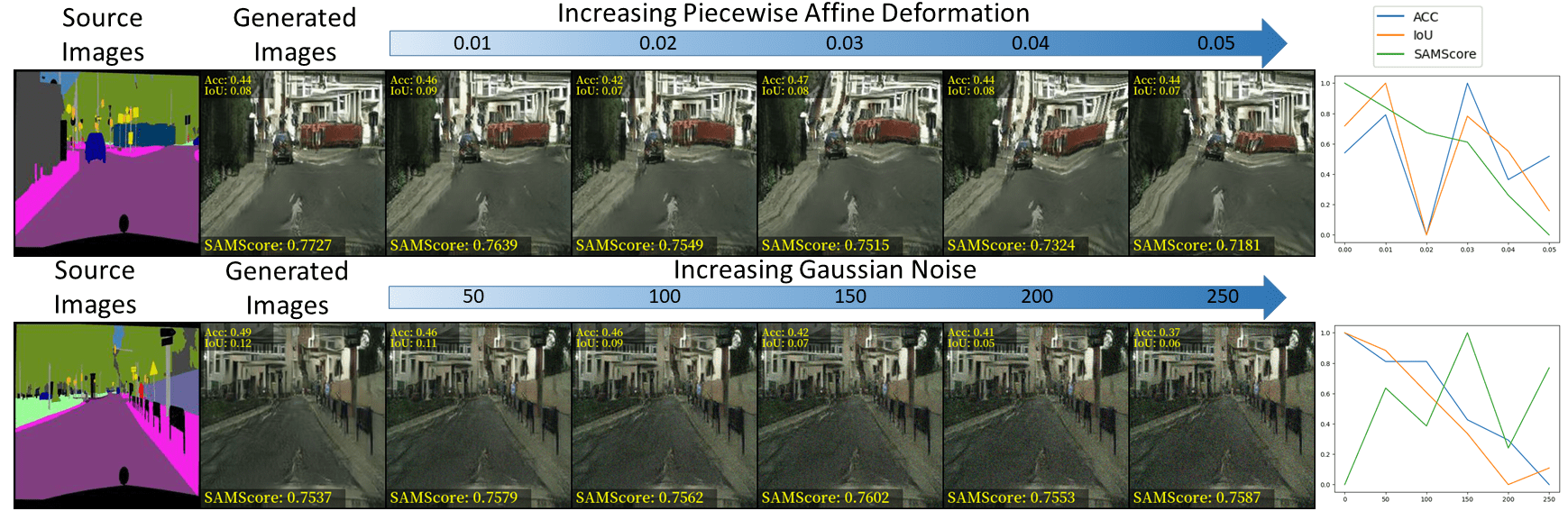
Figure 4: FCNScore and SAMScore: Piecewise affine deformations and Gaussian noises were applied to the generated images, then segmentation was performed by a DeepLabV3Plus that had been trained on target real images. The semantic structural similarity of the generated images was then evaluated by applying accuracy and IoU metrics. Column 2 shows results without added distortion. Given the varying scales of the different metrics, we standardized each metric to [0,1] before generating the line chart.

IV Experimental Setup

IV-A Datasets

We evaluated the performance of SAMScore on 19 image translation tasks across 8 datasets. The medical image dataset is from the MICCAI 2020 challenge on Anatomical Brain Barrier to Cancer Spread [28], while the other datasets were obtained from CycleGAN’s official public data repository [16]. The following is the list of image translation tasks considered in this paper: (1) apple to orange, (2) orange to apple, (3) cityscapes (label to photo), (4) cityscapes (photo to label), (5) facades (label to photo), (6) facades (photo to label), (7) head (MR to CT), (8) head (CT to MR), (9) horse to zebra, (10) zebra to horse, (11) Monet to photo, (12) photo to Monet, (13) aerial photograph to map, (14) map to aerial photograph, (15) photo to Cezanne, (16) photo to Ukiyoe, (17) photo to Vangogh, (18) Yosemite (summer to winter), and (19) Yosemite (winter to summer). We presented a detailed description of all datasets and tasks in Appendix A.

IV-B Evaluation Method

To assess the efficacy of SAMScore for measuring semantic structural similarity between source and generated images in image translation tasks, we conducted experiments introducing two types of distortions of the generated images: geometric deformations obtained via piecewise affine transformations [29], and additive Gaussian noises [30]. We varied the degree of each distortion and computed the absolute Pearson Correlation Coefficient between the resulting SAMScore and the level of distortion, as shown in Tables I and II. This allowed us to evaluate the sensitivity of SAMScore against different types of distortion, where a high correlation value indicates better sensitivity against distortion. Tables I and II also contain the correlation values obtained using L2, PSNR, SSIM, and LPIPS. The correlation values of FCNScore are reported in Table III. Absolute correlation values are reported since some metrics produce higher scores with increased similarity, and others produce lower scores. In Table I, a correlation coefficient closer to one implies higher sensitivity to affine distortion, which is desirable. In Table II, smaller correlations indicate less sensitivity to noise, which is also desirable. In the case of the head CT and MR data, the test data has ground truth images, so we additionally computed the L2 between the generated images and the ground truth images (Table IV).

IV-C Implementation Details

We conducted image translation tasks using the original CycleGAN structure and weights, with the exception of tasks 7 and 8 which utilized medical image data and were not included in the original CycleGAN experiments. For tasks 7 and 8, we re-trained the CycleGAN using its default parameters and also trained recent diffusion-based translation models. The diffusion model was trained following the standard setup in  [31], with a linear noise schedule ($\beta\in[1e-4,0.02]$) and 1000 diffusion steps. We used the Adam optimizer  [32] with a batch size of 16 and a learning rate of $10^{-4}$. An Exponential Moving Average (EMA) with a rate of 0.9999 was implemented to smooth the model parameters. We resized all images to a resolution of 256×256 pixels and added the piecewise affine deformations and Gaussian noise to the generated images using the widely used Albumentations data augmentation library [33] which enabled us to evaluate the sensitivity and robustness of the compared image similarity assessment metrics. To generate the piecewise affine deformations, each point on the regular grid was perturbed by a random amount drawn from a unit normal distribution but scaled in the range [0.01, 0.05], and the number of rows and columns of the regular grid is set to 4. The zero-mean additive Gaussian noise was drawn from a unit normal distribution scaled in the range [50, 250]. We used the originally published weights of the SAM (ViT-L) image encoders when embedding semantic structure, following the default SAM settings. Each image input to SAM was resampled to 1024×1024, while each embedded output from the SAM encoder was 64×64 with 256 channels. To calculate the FCNScores, we employed the DeepLabV3Plus-MobileNet segmentation model with pre-trained weights from a widely used open-source repository. Further details can be found in Appendix B.

V Results and Discussion

V-A Performance in the Presence of Piecewise Affine Deformations

We studied the relationship between each similarity metric against spatial deformations. The obtained Pearson Correlation Coefficients are tabulated in Table I. Among all the compared similarity metrics, SAMScore consistently exhibited the highest correlation coefficient with the degree of geometric (piecewise affine) deformation, highlighting its exceptional sensitivity to structural deformations and its efficacy in quantifying semantic structural similarity. Unlike L2, PSNR, and SSIM, which directly compute pixel-level or patch-level similarities between source and translated images, and are hence greatly influenced by low-level features such as color and texture, the SAM encoder used in SAMScore was trained on large semantic segmentation datasets to produce high-dimensional embeddings containing mainly image semantic structural information. LPIPS was not trained to interpret semantic structures, causing it to be less effective or robust.

Corresponding results for some of the tasks were visualized in Figure 2 to qualitatively support our findings. As the degree of piecewise affine deformation was increased, structural differences between the generated and source images become more pronounced. Unlike the other similarity metrics, SAMscore steadily decreased with increasing structural deformation, showing its sensitivity to semantic structural changes. More detailed results can be found in Appendix C.

V-B Performance in the Presence of Gaussian Noise

We distorted the translated images with varying levels of Gaussian noises, which have a negligible impact on the structural information of images when kept at a reasonable level. We measured the similarity scores of the generated images for each translation task using different metrics and calculated the corresponding Pearson correlation coefficients against the noise level. Table II summarizes the results. Our findings show that SAMScore is highly robust against Gaussian noise, as demonstrated by its consistently low correlation coefficients across most of the tasks. By contrast, traditional image similarity metrics including L2, PSNR, and SSIM exhibited strong correlations with the noise level. To supplement our quantitative results, we also provide visual comparisons of six image translation examples in Figure 3. The SAMScore values exhibit no apparent correlation with the degree of Gaussian noises.

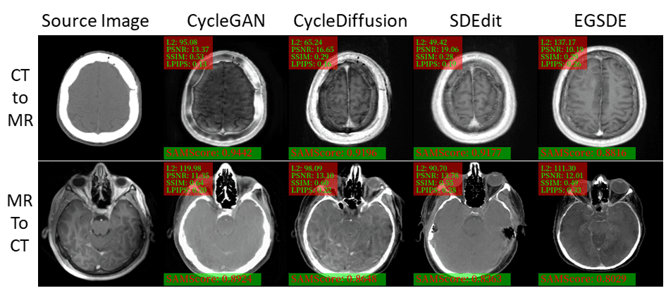
Figure 5: Evaluation of compared image similarity metrics on image translation tasks conducted by multiple state-of-the-art generative models, including CycleGAN, CycleDiffusion, SDEdit, and EGSDE, applied on head CT and MR images.

TABLE IV: Different similarity metrics on the medical image translation tasks (CT to MR and MR to CT). The arrows indicate the direction toward better performance.

Head MR to CT
Method	FID $\downarrow$	L2 $\downarrow$	PSNR $\uparrow$	SSIM $\uparrow$	LPIPS $\downarrow$	SAMScore $\uparrow$	L2 (GT) $\downarrow$
CycleGAN [16]	138.99	113.79	12.91	0.5786	0.2294	0.8861	76.39
CycleDiffusion [26]	85.42	89.06	15.13	0.5545	0.2290	0.8512	116.81
SDEdit [25]	122.53	75.64	16.59	0.5138	0.24833	0.8381	107.56
EGSDE [27]	118.48	127.17	11.07	0.4033	0.4172	0.7780	140.03
Head CT to MR
Method	FID $\downarrow$	L2 $\downarrow$	PSNR $\uparrow$	SSIM $\uparrow$	LPIPS $\downarrow$	SAMScore $\uparrow$	L2 (GT) $\downarrow$
CycleGAN [16]	138.29	108.79	12.63	0.5285	0.1855	0.9115	89.86
CycleDiffusion [26]	117.76	77.69	17.18	0.3908	0.1995	0.8904	111.22
SDEdit [25]	126.33	60.66	19.27	0.3505	0.2228	0.8734	112.62
EGSDE [27]	123.30	134.34	11.13	0.3744	0.4047	0.8101	133.36

V-C Comparison between SAMScore and FCNScore

In FCNScore, segmentation per-pixel accuracy (ACC) and mean class Intersection-Over-Union (IoU) using a pre-trained semantic segmentation network are two feasible measures of semantic structural similarity. To compare FCNScore against SAMScore, we obtained the segmentation ACC and IoU of the generated images using the FCN segmentation network (DeepLabV3Plus) on the cityscapes dataset, then compared the correlation coefficients of FCNScore and SAMScore against the amount of piecewise affine deformations and the degree of Gaussian noises. The results in Table III and Figure 4 show that SAMScore outperformed FCNScore in terms of accuracy and robustness. The inferior performance of FCNScore may be attributed to the following two factors. First, there is a domain gap between the training data and the testing data. The training of the segmentation network used real images from the ’true’ target domain, but the measurement of the semantic structure was performed on the generated images, which do not have the exact same distribution as the target images, resulting in large segmentation errors that affect ACC and IoU. Secondly, the granularity of the structure that FCNScore can evaluate is limited by the granularity of the segmentation labels. For example, the segmentation labels in the cityscapes dataset are specific to the entire object such as a car, but a car has a large number of structural details such as windows and lights. Using such coarse segmentation leads to the loss of critical information when comprehensively evaluating structural preservation and image similarity. Also, many image translation tasks do not have associated semantic segmentation labels, which limits the usefulness of FCNScore. More detailed results can be found in Appendix C.

V-D Performance on Different Translation Models

We also applied each of the similarity metrics to evaluate different image translation methods, for the purpose of assessing whether a metric is able to consistently measure the performance of image translation models. A medical image translation task (Head CT to MR and MR to CT translations) was used for this test. CycleGAN, the most widely used image translation benchmark, was evaluated. In comparison, the three diffusion-based methods, CycleDiffusion, SDEdit, and EGSDE, were also evaluated. From the visual comparison in Figure 5 and the L2 with ground truth (GT) in Table IV, the CycleGAN model appeared to preserve source structure the best, as it uses a consistency loss function to promote the retention of semantic information. The results in Table IV show that, based on the SAMScore, CycleGAN performed the best on both the CT to MR and the MR to CT translation tasks, which is consistent with visual evaluations and L2 (GT). The other metrics, especially L2 and PSNR, failed to provide consistent measurements with visual evaluation and L2 (GT). CT and MR present very different pixel values on the same underlying structures, rendering the pixel-based L2 and PSNR measures ineffective and highly error-prone. Among all faithfulness metrics, only the SAMScore ranking for each model is consistent with L2 (GT). The Frechet Inception Distance (FID) [34], a widely used metric for assessing realism, is computed by comparing a generated image dataset with a target domain dataset. Although the translation models based on diffusion produced less faithful results than CycleGAN, they performed better in terms of realism. This suggests that the joint optimization of FID and SAMScore could facilitate the emergence of translation models that perform better in terms of both faithfulness and realism.

VI Conclusion and Future Work

We presented SAMScore, a generic semantic structural similarity metric for evaluating image translation tasks. Our experimental results demonstrate that SAMScore substantially outperforms traditional metrics in terms of accuracy and robustness in evaluating semantic structural similarity. With the ability to better distinguish and evaluate translation models in terms of the retention of semantic structures, we believe that SAMScore has the potential to significantly contribute to the development of more effective techniques in the vibrant research area of image-to-image translation. We envision a variety of interesting avenues for future work, including the assessment of image structural similarity for specified regions of interest, and the development of SAMScore-guided image translation models.

Appendix A (Dataset Details)

Cityscapes dataset: The Cityscapes dataset [35] includes 2975 pairs of training images and 500 pairs of validation images. We used the validation set from Cityscapes for testing.

Maps and aerial photograph dataset: The dataset is from Google Maps [1], and includes 1096 pairs of training images and 1098 pairs of testing images. Images were sampled from in and around New York City.

Architectural facades dataset: The dataset is from the CMP Facade Database [36], including 400 pairs of training images and 106 pairs of testing images.

Horse and Zebra dataset: The dataset is from the ImageNet [37], including 939 images of the horse and 1177 images of the zebra for training. As for the testing set, there are 120 images of the horse and 140 images of the zebra.

Apple and Orange dataset: The dataset is from the ImageNet [37], including 996 apple and 1020 orange images for training, as well as 266 apple images and 248 orange images for testing.

Yosemite (summer and winter) dataset: The dataset is from Flickr [2], and the training set comprises 1273 summer images and 854 winter images, and the testing set has 309 summer images and 238 winter images.

Photo and Art dataset: The art images are from Wikiart [2]. The training set size of each class is 1074 (Monet), 584 (Cezanne), 401 (Vangogh), 1433 (Ukiyoe), and 6853 (Photo). The testing set size of each class is 121 (Monet), 58 (Cezanne), 400 (Vangogh), 263 (Ukiyoe), and 751 (Photo).

Head CT and MR dataset: The dataset is from the MICCAI 2020 challenge: Anatomical Brain Barrier to Cancer Spread [28]. MR is T1-weighted, and the training set contains 6390 CT and 6390 MR 2D slice images. The testing set has 1000 paired CT and MR 2D slice images.

Appendix B (Implementation Details)

SDEdit: SDEdit incorporates noise into the original image in forward diffusion, then proceeds to denoise the adulterated image with a diffusion model trained on the target domain during the reverse diffusion process. When performing inference, we add noise to the source image for 500 steps.

EGSDE: EGSDE utilizes an energy function, pre-trained on both the source and target domains, to direct the inference procedure in image translation. The energy function is decomposed into two terms, one of which encourages the transferred image to drop domain-specific features to obtain realism, and the other aims to retain domain-independent features to obtain faithfulness. When performing inference, we also add noise to the source image for 500 steps.

CycleDiffusion: This method proposes the unification of potential spaces of diffusion models, which is then utilized for cycle diffusion. For CycleDiffusion, a DDIM sampler with 100 steps is employed.

Appendix C (Detailed Experiment Results)

Piecewise Affine Deformation

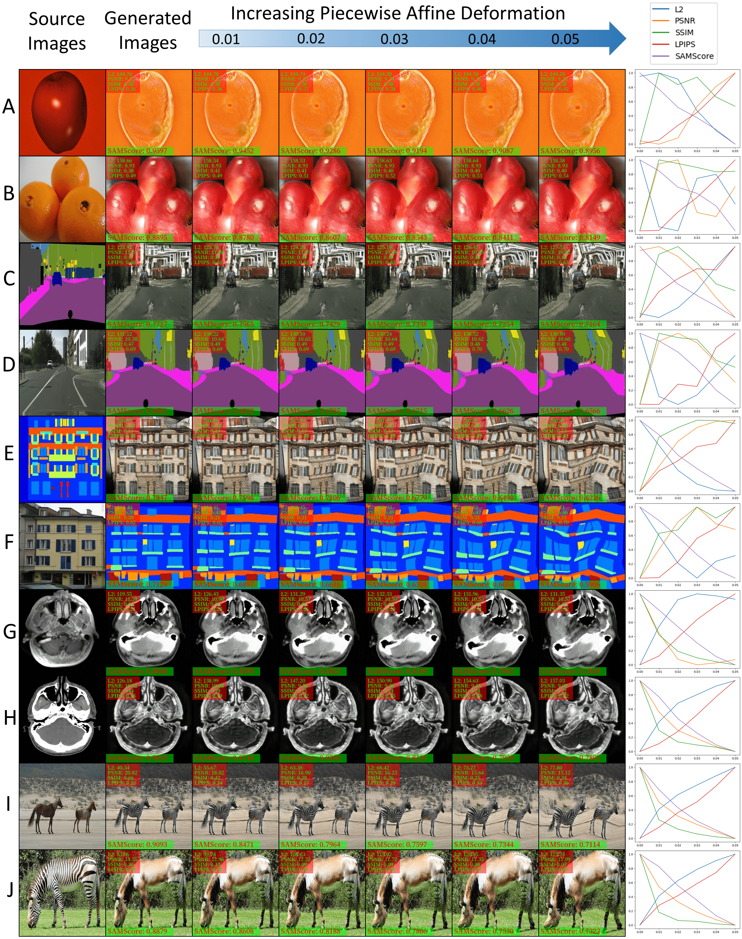
Figure 6: Similarity scores between the original images and CycleGAN-generated images with varying degrees of piecewise affine deformation. (A) apple to orange, (B) orange to apple, (C) cityscapes (label to photo), (D) cityscapes (photo to label), (E) facades (label to photo), (F) facades (photo to label), (G) head (MR to CT), (H) head (CT to MR), (I) horse to zebra, (J) zebra to horse. Column 2 shows results without additional distortion. Given the varying scales of the metrics, we standardized each metric to [0,1] before generating the line chart.

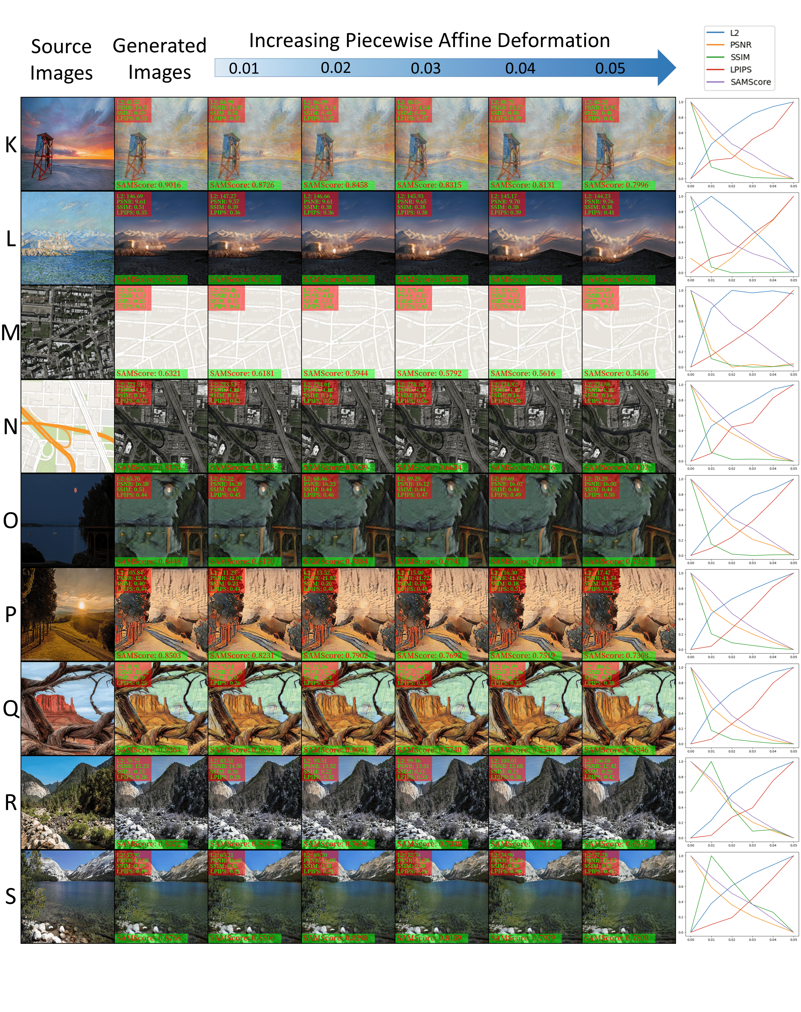
Figure 7: Similarity scores between the original images and CycleGAN-generated images with varying degrees of piecewise affine deformation. (K) photo to Monet, (L) Monet to photo, (M) aerial photograph to map, (N) map to aerial photograph, (O) photo to Cezanne, (P) photo to Ukiyoe, (Q) photo to Vangogh, (R) Yosemite (summer to winter), (S) Yosemite (winter to summer). Column 2 shows results without additional distortion. Given the varying scales of the metrics, we standardized each metric to [0,1] before generating the line chart.

Upon examining the experimental results displayed in Tables V, VI, VII, VIII, IX and Figures 6, 7, it is clear that our SAMScore is significantly more sensitive to geometric deformations than L2, PSNR, SSIM, and LPIPS. By observing the mean values of SAMScore for different tasks, we notice a general trend across all tasks. For each translation task, as the degree of piecewise affine deformation increased from 0 to 0.05, the SAMScore decreased correspondingly. This shows that SAMScore effectively captures the decrease in semantic structural similarity caused by the deformation, providing an accurate quantitative assessment of the level of deformation. In contrast, traditional similarity metrics such as L2, PSNR, SSIM, and LPIPS showed poor correlation for deformation. For example, in the ”cityscapes (label to photo)” task, L2 and PSNR distances barely correlate. While theoretically, structural similarity should decrease as the degree of deformation increases, SSIM is increasing on the ”apple to orange” task, showing the exact opposite wrong correlation, further demonstrating the inability of other metrics to accurately capture high-level semantic structure.

Gaussian Noise

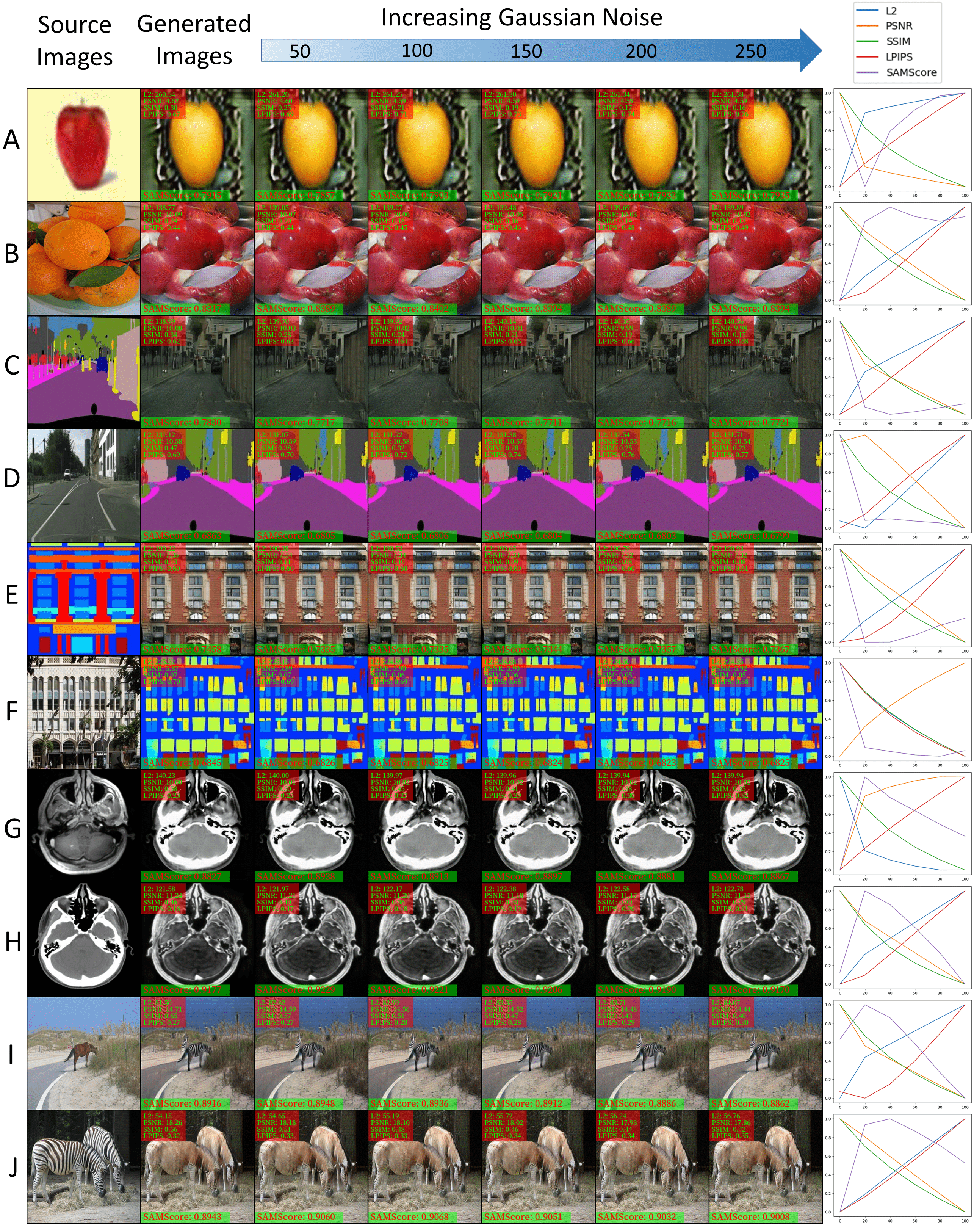
Figure 8: Similarity scores between the original images and CycleGAN-generated images with varying degrees of Gaussian noise corruption. (A) horse to zebra, (B) orange to apple, (C) cityscapes (label to photo), (D) head (MR to CT), (E) photo to Ukiyoe, and (F) photo to Monet. Column 2 shows results without additional distortion. Given the varying scales of the metrics, we standardized each metric to [0,1] before generating the line chart.

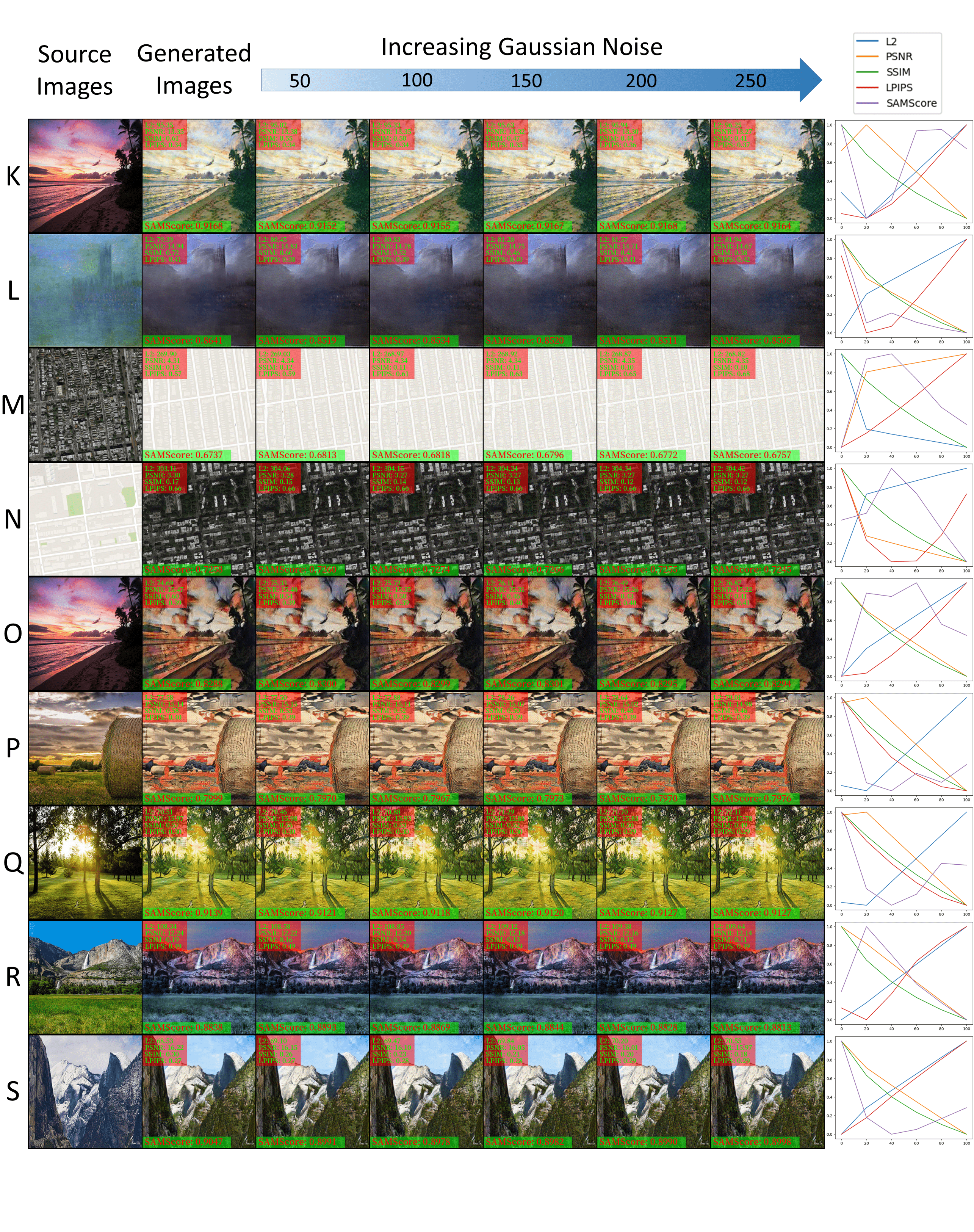
Figure 9: Similarity scores between the original images and CycleGAN-generated images with varying degrees of Gaussian noise corruption. (K) photo to Monet (L) Monet to photo (M) aerial photograph to map (N) map to aerial photograph (O) photo to Cezanne (P) photo to Ukiyoe (Q) photo to Vangogh (R) Yosemite (summer to winter) (S) Yosemite (winter to summer). Column 2 shows results without additional distortion. Given the varying scales of the metrics, we standardized each metric to [0,1] before generating the line chart.

Tables X, XI, XII, XIII, XIV display mean values for various image quality assessment metrics: L2, PSNR, SSIM, LPIPS, and our SAMScore results obtained from applying different degrees of Gaussian noise corruption to images from a variety of image translation tasks. Our proposed metric, SAMScore, proves to be robust to the noise added to images. As the degree of Gaussian noise increases, SAMScore exhibits the lowest correlation on most tasks. This shows that the semantic structure similarity measured by SAMScore is minimally affected by Gaussian noise, indicating its robustness as an indicator of faithfulness in image translation tasks. However, the other metrics show a clear correlation with increasing Gaussian noise, especially SSIM, as shown in Figures 8 and 9.

Appendix D (Comparison of SAMScore and FCNScore)

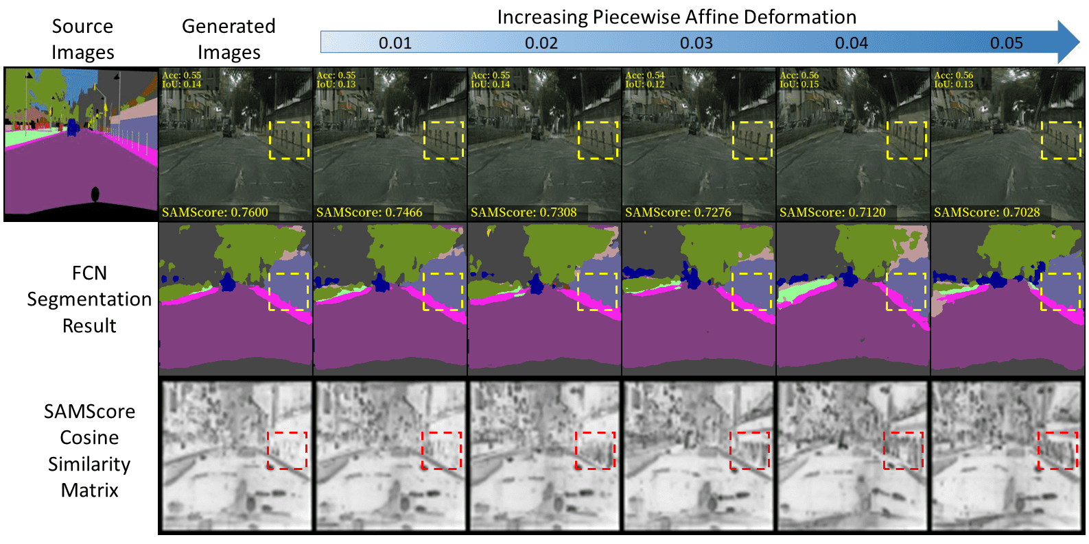
Figure 10: FCNScore and SAMScore: Piecewise affine deformations were applied to the generated images of the cityscapes (label to photo) task, then segmentation was performed by a FCN that had been trained on ”true” target images. The semantic structural similarity of the generated images was then evaluated by applying accuracy and IoU metrics. Column 2 shows results without added distortion. Row 2 shows the segmentation results of FCN, and row 3 shows the cosine similarity matrix of SAMScore.

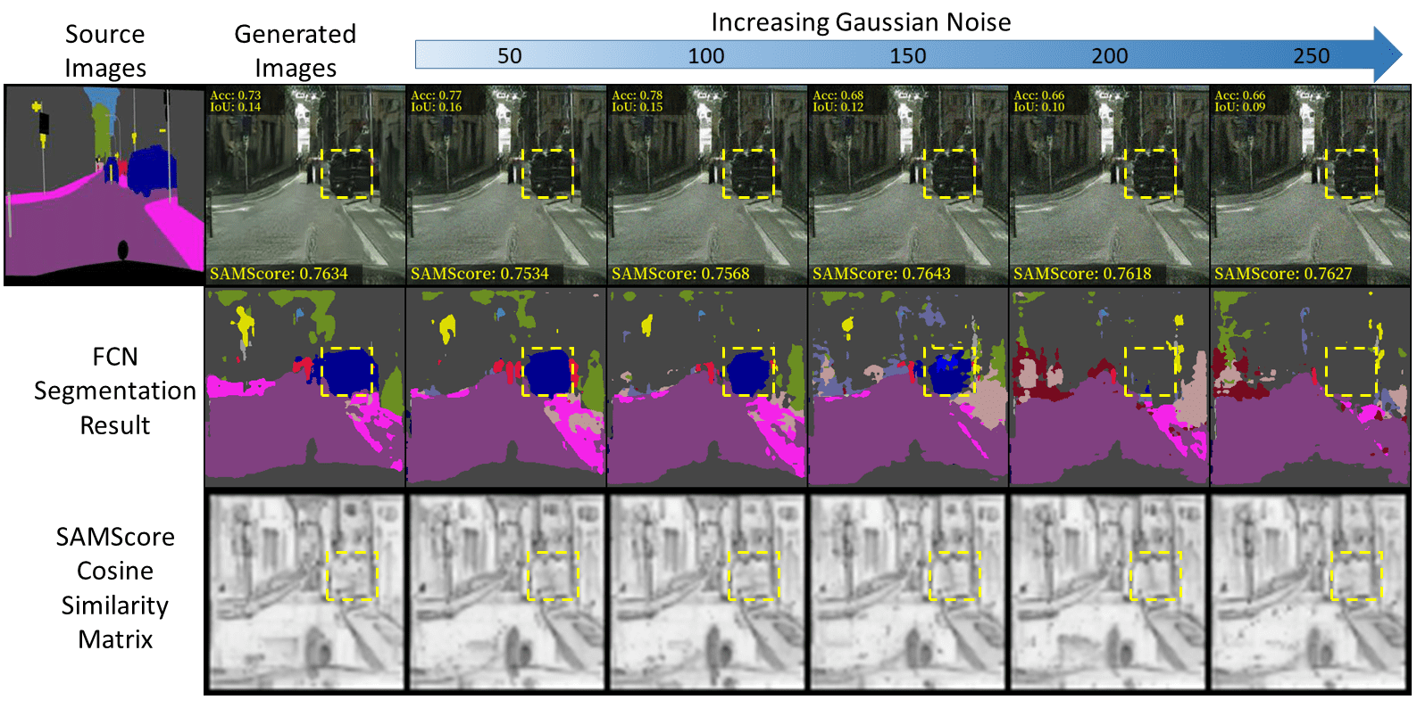
Figure 11: FCNScore and SAMScore: Gaussian noises were applied to the generated images of the cityscapes (label to photo) task, then segmentation was performed by a FCN that had been trained on ”true” target images. The semantic structural similarity of the generated images was then evaluated by applying accuracy and IoU metrics. Column 2 shows results without added distortion. Row 2 shows the segmentation results of FCN, and row 3 shows the cosine similarity matrix of SAMScore.

In Tables XV and XVI, we list the FCNScore (ACC and IoU) and SAMScore values for different degrees of piecewise affine distortion and Gaussian noise corruption on the cityscapes (label to photo) task. It can be seen from Table XVII that there is a large difference between the FCNScore on the translated image and on the target image, mainly because the FCN comes from the training of the ”true” target domain image, and it affects the segmentation accuracy of the translated image due to the significant difference between the target image and the translated image. In the cosine similarity matrix of SAMScore, brighter positions represent higher similarity, and darker positions represent lower similarity. Looking at the road safety posts in the dotted box in Figure 10, the FCN cannot correctly segment them, resulting in inaccurate evaluation. The similarity matrix of our SAMScore changes with the increase of the deformation, the position and shape of the road safety posts, and the similarity with the source image here is also gradually decreasing, which proves that our SAMScore not only correctly extracts their semantic structure and can identify differences very sensitively. In Figure 11, the segmentation accuracy of FCN keeps decreasing with the increase of Gaussian noise, while our SAMScore shows higher robustness. The sensitivity and robustness of SAMScore to such distortions and its ability to outperform traditional FCN-based measures suggest that it has the potential to be a valuable tool for evaluating and developing more sophisticated image translation models.

TABLE V: Mean values of L2 for different tasks with different degrees of piecewise affine deformation.

Degree of Deformation	0	0.01	0.02	0.03	0.04	0.05
apple to orange	221.14	219.51	217.80	216.64	215.23	213.98
orange to apple	231.25	229.41	227.52	225.75	224.41	223.19
cityscapes (label to photo)	120.69	120.02	119.99	120.35	120.69	121.06
cityscapes (photo to label)	118.18	117.89	117.94	118.08	118.31	118.54
facades (label to photo)	214.29	213.26	212.14	211.38	211.05	210.44
facades (photo to label)	208.67	207.92	207.08	206.35	205.85	205.21
head (MR to CT)	113.79	115.02	116.38	117.34	118.61	120.57
head (CT to MR)	108.79	115.32	120.06	123.10	125.85	128.19
horse to zebra	54.98	66.14	74.53	79.72	83.98	86.87
zebra to horse	61.08	73.19	82.09	87.66	91.74	95.13
photo to Monet	63.98	77.29	82.56	85.60	89.04	91.06
Monet to photo	74.77	85.08	90.40	93.89	96.75	99.10
aerial photograph to map	283.04	283.40	283.62	283.73	283.77	283.82
map to aerial photograph	293.06	293.47	293.70	293.82	293.91	293.96
photo to Cezanne	60.84	71.09	77.44	81.97	85.73	88.22
photo to Ukiyoe	102.20	111.09	116.00	119.32	122.04	123.96
photo to Vangogh	72.68	84.34	90.25	93.99	96.89	99.17
Yosemite (summer to winter)	72.00	74.68	80.34	84.83	88.08	91.13
Yosemite (winter to summer)	73.72	77.98	84.51	88.63	92.38	95.32

TABLE VI: Mean values of PSNR for different tasks with different degrees of piecewise affine deformation.

Degree of Deformation	0	0.01	0.02	0.03	0.04	0.05
apple to orange	6.31	6.38	6.45	6.51	6.56	6.62
orange to apple	5.96	6.03	6.11	6.19	6.24	6.29
cityscapes (label to photo)	11.36	11.41	11.41	11.38	11.35	11.33
cityscapes (photo to label)	11.56	11.58	11.57	11.56	11.55	11.53
facades (label to photo)	6.34	6.38	6.43	6.46	6.47	6.50
facades (photo to label)	6.56	6.59	6.62	6.65	6.68	6.70
head (MR to CT)	12.91	12.83	12.73	12.67	12.58	12.46
head (CT to MR)	12.63	12.09	11.74	11.51	11.31	11.15
horse to zebra	18.51	16.79	15.71	15.09	14.63	14.33
zebra to horse	17.54	15.91	14.88	14.32	13.91	13.58
photo to Monet	17.92	15.59	14.92	14.56	14.19	13.98
Monet to photo	16.08	14.70	14.11	13.75	13.46	13.24
aerial photograph to map	3.91	3.90	3.90	3.89	3.89	3.89
map to aerial photograph	3.61	3.59	3.59	3.58	3.58	3.58
photo to Cezanne	17.52	16.05	15.29	14.79	14.40	14.15
photo to Ukiyoe	12.96	12.17	11.78	11.52	11.32	11.18
photo to Vangogh	15.90	14.52	13.92	13.56	13.29	13.09
Yosemite (summer to winter)	16.15	15.81	15.12	14.61	14.27	13.96
Yosemite (winter to summer)	15.92	15.40	14.66	14.24	13.85	13.57

TABLE VII: Mean values of SSIM for different tasks with different degrees of piecewise affine deformation.

Degree of Deformation	0	0.01	0.02	0.03	0.04	0.05
apple to orange	0.2166	0.2539	0.2709	0.2769	0.2809	0.2835
orange to apple	0.1646	0.2062	0.2243	0.2321	0.2352	0.2386
cityscapes (label to photo)	0.3675	0.3856	0.3889	0.3876	0.3864	0.3849
cityscapes (photo to label)	0.4447	0.4532	0.4544	0.4545	0.4545	0.4537
facades (label to photo)	0.1390	0.1575	0.1631	0.1639	0.1644	0.1643
facades (photo to label)	0.1732	0.1805	0.1827	0.1840	0.1837	0.1846
head (MR to CT)	0.5786	0.5232	0.4964	0.4866	0.4796	0.4730
head (CT to MR)	0.5285	0.4510	0.4200	0.4088	0.4014	0.3951
horse to zebra	0.6226	0.4251	0.3688	0.3531	0.3385	0.3333
zebra to horse	0.5734	0.3760	0.3115	0.2894	0.2780	0.2690
photo to Monet	0.7228	0.3911	0.3404	0.3222	0.3123	0.3080
Monet to photo	0.6519	0.4011	0.3542	0.3380	0.3292	0.3241
aerial photograph to map	0.1646	0.1444	0.1386	0.1372	0.1368	0.1366
map to aerial photograph	0.1775	0.1480	0.1421	0.1411	0.1409	0.1410
photo to Cezanne	0.6176	0.4137	0.3657	0.3470	0.3368	0.3302
photo to Ukiyoe	0.5485	0.3318	0.2949	0.2816	0.2745	0.2707
photo to Vangogh	0.5477	0.2978	0.2529	0.2402	0.2340	0.2295
Yosemite (summer to winter)	0.3797	0.4149	0.3754	0.3584	0.3488	0.3423
Yosemite (winter to summer)	0.3541	0.3735	0.3415	0.3267	0.3161	0.3098

TABLE VIII: Mean values of LPIPS for different tasks with different degrees of piecewise affine deformation.

Degree of Deformation	0	0.01	0.02	0.03	0.04	0.05
apple to orange	0.5076	0.5128	0.5219	0.5350	0.5477	0.5612
orange to apple	0.5133	0.5211	0.5333	0.5474	0.5615	0.5739
cityscapes (label to photo)	0.5835	0.5855	0.5901	0.5963	0.6018	0.6073
cityscapes (photo to label)	0.6310	0.6305	0.6319	0.6345	0.6389	0.6428
facades (label to photo)	0.6424	0.6444	0.6492	0.6570	0.6626	0.6724
facades (photo to label)	0.6590	0.6598	0.6643	0.6699	0.6753	0.6849
head (MR to CT)	0.2294	0.2388	0.2536	0.2722	0.2901	0.3094
head (CT to MR)	0.1855	0.1952	0.2098	0.2272	0.2475	0.2662
horse to zebra	0.2696	0.2830	0.3012	0.3236	0.3496	0.3733
zebra to horse	0.3231	0.3391	0.3598	0.3831	0.4026	0.4278
photo to Monet	0.2512	0.2796	0.2990	0.3210	0.3500	0.3693
Monet to photo	0.2708	0.2943	0.3136	0.3367	0.3609	0.3848
aerial photograph to map	0.6038	0.6055	0.6095	0.6154	0.6220	0.6296
map to aerial photograph	0.6070	0.6120	0.6187	0.6244	0.6292	0.6344
photo to Cezanne	0.3789	0.3940	0.4082	0.4262	0.4456	0.4633
photo to Ukiyoe	0.4157	0.4308	0.4440	0.4591	0.4781	0.4946
photo to Vangogh	0.4146	0.4307	0.4440	0.4598	0.4779	0.4947
Yosemite (summer to winter)	0.2603	0.2704	0.2927	0.3189	0.3473	0.3744
Yosemite (winter to summer)	0.2674	0.2783	0.3032	0.3270	0.3573	0.3857

TABLE IX: Mean values of SAMScore for different tasks with different degrees of piecewise affine deformation.

Degree of Deformation	0	0.01	0.02	0.03	0.04	0.05
apple to orange	0.8266	0.8105	0.7923	0.7774	0.7651	0.7542
orange to apple	0.8401	0.8228	0.8021	0.7847	0.7695	0.7568
cityscapes (label to photo)	0.7624	0.7499	0.7364	0.7246	0.7161	0.7083
cityscapes (photo to label)	0.6845	0.6850	0.6811	0.6759	0.6691	0.6631
facades (label to photo)	0.7695	0.7443	0.7118	0.6880	0.6697	0.6527
facades (photo to label)	0.6923	0.6773	0.6572	0.6396	0.6230	0.6113
head (MR to CT)	0.8861	0.8757	0.8608	0.8484	0.8378	0.8280
head (CT to MR)	0.9115	0.8956	0.8768	0.8622	0.8497	0.8398
horse to zebra	0.8943	0.8603	0.8265	0.8047	0.7865	0.7713
zebra to horse	0.8949	0.8613	0.8258	0.8010	0.7833	0.7663
photo to Monet	0.9054	0.8669	0.8377	0.8184	0.8000	0.7890
Monet to photo	0.9170	0.8774	0.8446	0.8220	0.8043	0.7889
aerial photograph to map	0.6734	0.6553	0.6330	0.6185	0.6089	0.6011
map to aerial photograph	0.7542	0.7154	0.6820	0.6595	0.6450	0.6356
photo to Cezanne	0.8511	0.8179	0.7902	0.7707	0.7554	0.7444
photo to Ukiyoe	0.8139	0.7788	0.7499	0.7318	0.7186	0.7098
photo to Vangogh	0.8510	0.8133	0.7828	0.7640	0.7500	0.7375
Yosemite (summer to winter)	0.8878	0.8677	0.8395	0.8180	0.8000	0.7855
Yosemite (winter to summer)	0.8952	0.8672	0.8347	0.8143	0.7952	0.7815

TABLE X: Mean values of L2 for different tasks with different degrees of Gaussian noise corruption.

Degree of Gaussian Noise	0	50	100	150	200	250
apple to orange	221.14	221.27	221.33	221.40	221.46	221.53
orange to apple	231.25	231.25	231.17	231.11	231.05	231.02
cityscapes (label to photo)	120.69	121.35	121.91	122.46	122.98	123.50
cityscapes (photo to label)	118.18	118.30	118.74	119.19	119.65	120.12
facades (label to photo)	214.29	214.50	214.76	215.03	215.29	215.55
facades (photo to label)	208.67	207.53	206.89	206.41	206.03	205.70
head (MR to CT)	113.79	113.59	113.70	113.86	114.05	114.26
head (CT to MR)	108.79	109.48	110.02	110.54	111.06	111.57
horse to zebra	54.98	56.59	57.96	59.26	60.53	61.75
zebra to horse	61.08	62.30	63.54	64.74	65.89	67.01
photo to Monet	63.98	65.92	67.24	68.49	69.67	70.80
Monet to photo	74.77	75.36	76.49	77.57	78.64	79.68
aerial photograph to map	283.04	282.07	281.97	281.84	281.67	281.48
map to aerial photograph	293.06	294.16	294.38	294.57	294.74	294.89
photo to Cezanne	60.84	62.17	63.41	64.60	65.77	66.89
photo to Ukiyoe	102.20	102.38	103.11	103.82	104.52	105.19
photo to Vangogh	72.68	73.60	74.63	75.63	76.61	77.57
Yosemite (summer to winter)	72.00	72.99	74.04	75.05	76.02	76.95
Yosemite (winter to summer)	73.72	74.90	75.89	76.83	77.74	78.63

TABLE XI: Mean values of PSNR for different tasks with different degrees of Gaussian noise corruption.

Degree of Gaussian Noise	0	50	100	150	200	250
apple to orange	6.31	6.30	6.30	6.29	6.29	6.28
orange to apple	5.96	5.95	5.95	5.95	5.95	5.95
cityscapes (label to photo)	11.36	11.31	11.27	11.23	11.19	11.15
cityscapes (photo to label)	11.56	11.55	11.51	11.48	11.44	11.41
facades (label to photo)	6.34	6.33	6.32	6.31	6.30	6.28
facades (photo to label)	6.56	6.61	6.63	6.65	6.67	6.68
head (MR to CT)	12.91	12.64	12.54	12.48	12.42	12.37
head (CT to MR)	12.63	12.51	12.44	12.39	12.33	12.28
horse to zebra	18.51	18.23	17.99	17.77	17.57	17.37
zebra to horse	17.54	17.34	17.14	16.96	16.79	16.62
photo to Monet	17.92	17.52	17.24	17.01	16.80	16.60
Monet to photo	16.08	15.97	15.81	15.66	15.51	15.37
aerial photograph to map	3.91	3.94	3.95	3.95	3.96	3.96
map to aerial photograph	3.61	3.57	3.57	3.56	3.56	3.55
photo to Cezanne	17.52	17.31	17.12	16.94	16.77	16.61
photo to Ukiyoe	12.96	12.94	12.87	12.80	12.74	12.68
photo to Vangogh	15.90	15.78	15.65	15.53	15.41	15.29
Yosemite (summer to winter)	16.15	16.01	15.87	15.73	15.60	15.48
Yosemite (winter to summer)	15.92	15.76	15.63	15.51	15.39	15.28

TABLE XII: Mean values of SSIM for different tasks with different degrees of Gaussian noise corruption.

Degree of Gaussian Noise	0	50	100	150	200	250
apple to orange	0.2166	0.1394	0.1041	0.0829	0.0687	0.0585
orange to apple	0.1646	0.1051	0.0774	0.0608	0.0496	0.0414
cityscapes (label to photo)	0.3675	0.2394	0.1822	0.1483	0.1254	0.1089
cityscapes (photo to label)	0.4447	0.2923	0.2253	0.1858	0.1593	0.1400
facades (label to photo)	0.1390	0.0967	0.0756	0.0622	0.0527	0.0457
facades (photo to label)	0.1732	0.1345	0.1148	0.1017	0.0921	0.0846
head (MR to CT)	0.5786	0.4453	0.3662	0.3156	0.2796	0.2525
head (CT to MR)	0.5285	0.3370	0.2639	0.2230	0.1959	0.1763
horse to zebra	0.6226	0.4915	0.4215	0.3751	0.3405	0.3139
zebra to horse	0.5734	0.4653	0.4053	0.3644	0.3337	0.3094
photo to Monet	0.7228	0.5856	0.5100	0.4585	0.4198	0.3895
Monet to photo	0.6519	0.5203	0.4481	0.3997	0.3639	0.3359
aerial photograph to map	0.1646	0.1314	0.1137	0.1019	0.0933	0.0867
map to aerial photograph	0.1775	0.1400	0.1200	0.1065	0.0965	0.0887
photo to Cezanne	0.6176	0.4892	0.4195	0.3730	0.3387	0.3122
photo to Ukiyoe	0.5485	0.4465	0.3916	0.3548	0.3275	0.3059
photo to Vangogh	0.5477	0.4673	0.4177	0.3821	0.3545	0.3322
Yosemite (summer to winter)	0.3797	0.2695	0.2177	0.1861	0.1641	0.1477
Yosemite (winter to summer)	0.3541	0.2552	0.2084	0.1795	0.1593	0.1442

TABLE XIII: Mean values of LPIPS for different tasks with different degrees of Gaussian noise corruption.

Degree of Gaussian Noise	0	50	100	150	200	250
apple to orange	0.5076	0.5369	0.5700	0.5976	0.6194	0.6385
orange to apple	0.5133	0.5479	0.5775	0.6017	0.6218	0.6395
cityscapes (label to photo)	0.5835	0.6048	0.6337	0.6581	0.6786	0.6974
cityscapes (photo to label)	0.6310	0.6726	0.7159	0.7481	0.7725	0.7923
facades (label to photo)	0.6424	0.6469	0.6538	0.6623	0.6708	0.6797
facades (photo to label)	0.6590	0.6544	0.6570	0.6624	0.6687	0.6758
head (MR to CT)	0.2294	0.3150	0.3726	0.4151	0.4491	0.4765
head (CT to MR)	0.1855	0.2353	0.2765	0.3076	0.3339	0.3565
horse to zebra	0.2696	0.2842	0.3040	0.3210	0.3382	0.3538
zebra to horse	0.3231	0.3429	0.3678	0.3902	0.4117	0.4310
photo to Monet	0.2512	0.2428	0.2562	0.2728	0.2896	0.3066
Monet to photo	0.2708	0.2947	0.3224	0.3475	0.3699	0.3911
aerial photograph to map	0.6038	0.6233	0.6683	0.7131	0.7531	0.7873
map to aerial photograph	0.6070	0.6137	0.6211	0.6289	0.6366	0.6439
photo to Cezanne	0.3789	0.3806	0.3898	0.4002	0.4114	0.4226
photo to Ukiyoe	0.4157	0.4182	0.4245	0.4314	0.4383	0.4454
photo to Vangogh	0.4146	0.4151	0.4184	0.4232	0.4286	0.4346
Yosemite (summer to winter)	0.2603	0.2805	0.3057	0.3286	0.3492	0.3678
Yosemite (winter to summer)	0.2674	0.2863	0.3092	0.3310	0.3507	0.3684

TABLE XIV: Mean values of SAMScore for different tasks with different degrees of Gaussian noise corruption.

Degree of Gaussian Noise	0	50	100	150	200	250
apple to orange	0.8266	0.8225	0.8214	0.8203	0.8189	0.8190
orange to apple	0.8401	0.8338	0.8314	0.8300	0.8281	0.8270
cityscapes (label to photo)	0.7624	0.7477	0.7501	0.7531	0.7560	0.7579
cityscapes (photo to label)	0.6845	0.6775	0.6772	0.6778	0.6784	0.6792
facades (label to photo)	0.7695	0.7695	0.7722	0.7739	0.7762	0.7774
facades (photo to label)	0.6923	0.6866	0.6852	0.6843	0.6835	0.6829
head (MR to CT)	0.8861	0.8795	0.8759	0.8736	0.8716	0.8702
head (CT to MR)	0.9115	0.9341	0.9309	0.9287	0.9270	0.9254
horse to zebra	0.8943	0.8888	0.8850	0.8815	0.8791	0.8774
zebra to horse	0.8949	0.8944	0.8903	0.8872	0.8836	0.8798
photo to Monet	0.9054	0.8925	0.8884	0.8849	0.8828	0.8808
Monet to photo	0.9170	0.9134	0.9095	0.9063	0.9032	0.9003
aerial photograph to map	0.6734	0.6522	0.6395	0.6319	0.6270	0.6235
map to aerial photograph	0.7542	0.7602	0.7568	0.7534	0.7510	0.7489
photo to Cezanne	0.8511	0.8420	0.8382	0.8360	0.8339	0.8330
photo to Ukiyoe	0.8139	0.8140	0.8138	0.8141	0.8148	0.8152
photo to Vangogh	0.8510	0.8491	0.8491	0.8492	0.8493	0.8497
Yosemite (summer to winter)	0.8878	0.8851	0.8803	0.8760	0.8732	0.8702
Yosemite (winter to summer)	0.8952	0.8900	0.8849	0.8811	0.8784	0.8758

TABLE XV: FCNScore (ACC and IoU) and SAMScore of translated images with different degrees of piecewise affine deformation.

Degree of Deformation	0	0.01	0.02	0.03	0.04	0.05
Per-pixel ACC	0.5055	0.5055	0.5004	0.4973	0.4894	0.4828
Class IoU	0.1248	0.1222	0.1175	0.1122	0.1049	0.0993
SAMScore	0.7624	0.7498	0.7361	0.7247	0.7174	0.7091

TABLE XVI: FCNScore (ACC and IoU) and SAMScore of translated images with different degrees of Gaussian noise corruption.

Degree of Gaussian Noise	0	50	100	150	200	250
Per-pixel ACC	0.5055	0.5013	0.4893	0.4714	0.4537	0.4402
Class IoU	0.1248	0.1184	0.1087	0.0990	0.0896	0.0813
SAMScore	0.7624	0.7476	0.7504	0.7530	0.7558	0.7574

TABLE XVII: FCNScore (ACC and IoU) on target images and translated images. FCN is trained on ’true’ target domain images, and the cause for the large differences in FCNScore between the target image and the translated image is the presence of the domain gap (between the ’true’ target image domain and the translated image domain), which affects the segmentation accuracy on the translated images.

	Target Image	Translated Image
Per-pixel ACC	0.8433	0.5055
Class IoU	0.2711	0.1248

References

- [1] P. Isola, J.-Y. Zhu, T. Zhou, and A. A. Efros, “Image-to-image translation with conditional adversarial networks,” in Proceedings of the IEEE conference on computer vision and pattern recognition, 2017, pp. 1125–1134.
- [2] M.-Y. Liu, T. Breuel, and J. Kautz, “Unsupervised image-to-image translation networks,” Advances in neural information processing systems, vol. 30, 2017.
- [3] J.-Y. Zhu, R. Zhang, D. Pathak, T. Darrell, A. A. Efros, O. Wang, and E. Shechtman, “Toward multimodal image-to-image translation,” Advances in neural information processing systems, vol. 30, 2017.
- [4] Y. Choi, M. Choi, M. Kim, J.-W. Ha, S. Kim, and J. Choo, “Stargan: Unified generative adversarial networks for multi-domain image-to-image translation,” in Proceedings of the IEEE conference on computer vision and pattern recognition, 2018, pp. 8789–8797.
- [5] E. Richardson, Y. Alaluf, O. Patashnik, Y. Nitzan, Y. Azar, S. Shapiro, and D. Cohen-Or, “Encoding in style: a stylegan encoder for image-to-image translation,” in Proceedings of the IEEE/CVF conference on computer vision and pattern recognition, 2021, pp. 2287–2296.
- [6] K. Armanious, C. Jiang, M. Fischer, T. Küstner, T. Hepp, K. Nikolaou, S. Gatidis, and B. Yang, “Medgan: Medical image translation using gans,” Computerized medical imaging and graphics, vol. 79, p. 101684, 2020.
- [7] Y. Pang, J. Lin, T. Qin, and Z. Chen, “Image-to-image translation: Methods and applications,” IEEE Transactions on Multimedia, vol. 24, pp. 3859–3881, 2021.
- [8] S. Kaji and S. Kida, “Overview of image-to-image translation by use of deep neural networks: denoising, super-resolution, modality conversion, and reconstruction in medical imaging,” Radiological physics and technology, vol. 12, pp. 235–248, 2019.
- [9] A. Alotaibi, “Deep generative adversarial networks for image-to-image translation: A review,” Symmetry, vol. 12, no. 10, p. 1705, 2020.
- [10] M. Arar, Y. Ginger, D. Danon, A. H. Bermano, and D. Cohen-Or, “Unsupervised multi-modal image registration via geometry preserving image-to-image translation,” in Proceedings of the IEEE/CVF conference on computer vision and pattern recognition, 2020, pp. 13 410–13 419.
- [11] R. Zhang, P. Isola, A. A. Efros, E. Shechtman, and O. Wang, “The unreasonable effectiveness of deep features as a perceptual metric,” in Proceedings of the IEEE conference on computer vision and pattern recognition, 2018, pp. 586–595.
- [12] A. Borji, “Pros and cons of gan evaluation measures,” Computer Vision and Image Understanding, vol. 179, pp. 41–65, 2019.
- [13] D. Bashkirova, B. Usman, and K. Saenko, “Evaluation of correctness in unsupervised many-to-many image translation,” in Proceedings of the IEEE/CVF Winter Conference on Applications of Computer Vision, 2022, pp. 1776–1785.
- [14] Z. Wang, A. C. Bovik, H. R. Sheikh, and E. P. Simoncelli, “Image quality assessment: from error visibility to structural similarity,” IEEE transactions on image processing, vol. 13, no. 4, pp. 600–612, 2004.
- [15] A. Lahouhou, E. Viennet, and A. Beghdadi, “Selecting low-level features for image quality assessment by statistical methods,” Journal of computing and information technology, vol. 18, no. 2, pp. 183–189, 2010.
- [16] J.-Y. Zhu, T. Park, P. Isola, and A. A. Efros, “Unpaired image-to-image translation using cycle-consistent adversarial networks,” in Proceedings of the IEEE international conference on computer vision, 2017, pp. 2223–2232.
- [17] A. Kirillov, E. Mintun, N. Ravi, H. Mao, C. Rolland, L. Gustafson, T. Xiao, S. Whitehead, A. C. Berg, W.-Y. Lo et al., “Segment anything,” arXiv preprint arXiv:2304.02643, 2023.
- [18] J. Ma and B. Wang, “Segment anything in medical images,” arXiv preprint arXiv:2304.12306, 2023.
- [19] Y. Zhang, S. Wang, B. Chen, and J. Cao, “Gcgan: Generative adversarial nets with graph cnn for network-scale traffic prediction,” in 2019 International Joint Conference on Neural Networks (IJCNN). IEEE, 2019, pp. 1–8.
- [20] T. Park, A. A. Efros, R. Zhang, and J.-Y. Zhu, “Contrastive learning for unpaired image-to-image translation,” in Computer Vision–ECCV 2020: 16th European Conference, Glasgow, UK, August 23–28, 2020, Proceedings, Part IX 16. Springer, 2020, pp. 319–345.
- [21] X. Huang, M.-Y. Liu, S. Belongie, and J. Kautz, “Multimodal unsupervised image-to-image translation,” in Proceedings of the European conference on computer vision (ECCV), 2018, pp. 172–189.
- [22] Y. Choi, Y. Uh, J. Yoo, and J.-W. Ha, “Stargan v2: Diverse image synthesis for multiple domains,” in Proceedings of the IEEE/CVF conference on computer vision and pattern recognition, 2020, pp. 8188–8197.
- [23] G. Paolacci, J. Chandler, and P. G. Ipeirotis, “Running experiments on amazon mechanical turk,” Judgment and Decision making, vol. 5, no. 5, pp. 411–419, 2010.
- [24] B. Li, K. Xue, B. Liu, and Y.-K. Lai, “Vqbb: Image-to-image translation with vector quantized brownian bridge,” arXiv preprint arXiv:2205.07680, 2022.
- [25] C. Meng, Y. He, Y. Song, J. Song, J. Wu, J.-Y. Zhu, and S. Ermon, “Sdedit: Guided image synthesis and editing with stochastic differential equations,” in International Conference on Learning Representations, 2021.
- [26] C. H. Wu and F. De la Torre, “Unifying diffusion models’ latent space, with applications to cyclediffusion and guidance,” arXiv preprint arXiv:2210.05559, 2022.
- [27] M. Zhao, F. Bao, C. Li, and J. Zhu, “Egsde: Unpaired image-to-image translation via energy-guided stochastic differential equations,” arXiv preprint arXiv:2207.06635, 2022.
- [28] N. Shusharina, M. P. Heinrich, and R. Huang, Segmentation, Classification, and Registration of Multi-modality Medical Imaging Data: MICCAI 2020 Challenges, ABCs 2020, L2R 2020, TN-SCUI 2020, Held in Conjunction with MICCAI 2020, Lima, Peru, October 4–8, 2020, Proceedings. Springer Nature, 2021, vol. 12587.
- [29] A. Pitiot, G. Malandain, E. Bardinet, and P. M. Thompson, “Piecewise affine registration of biological images,” in Biomedical Image Registration: Second InternationalWorkshop, WBIR 2003, Philadelphia, PA, USA, June 23-24, 2003. Revised Papers 2. Springer, 2003, pp. 91–101.
- [30] A. K. Qin and D. A. Clausi, “Multivariate image segmentation using semantic region growing with adaptive edge penalty,” IEEE transactions on image processing, vol. 19, no. 8, pp. 2157–2170, 2010.
- [31] A. Q. Nichol and P. Dhariwal, “Improved denoising diffusion probabilistic models,” in International Conference on Machine Learning, 2021, pp. 8162–8171.
- [32] D. P. Kingma and J. Ba, “Adam: A method for stochastic optimization,” in International Conference on Learning Representations, 2014.
- [33] A. Buslaev, V. I. Iglovikov, E. Khvedchenya, A. Parinov, M. Druzhinin, and A. A. Kalinin, “Albumentations: fast and flexible image augmentations,” Information, vol. 11, no. 2, p. 125, 2020.
- [34] M. Heusel, H. Ramsauer, T. Unterthiner, B. Nessler, and S. Hochreiter, “Gans trained by a two time-scale update rule converge to a local nash equilibrium,” Advances in neural information processing systems, vol. 30, 2017.
- [35] M. Cordts, M. Omran, S. Ramos, T. Rehfeld, M. Enzweiler, R. Benenson, U. Franke, S. Roth, and B. Schiele, “The cityscapes dataset for semantic urban scene understanding,” in Proceedings of the IEEE conference on computer vision and pattern recognition, 2016, pp. 3213–3223.
- [36] R. Tyleček and R. Šára, “Spatial pattern templates for recognition of objects with regular structure,” in Pattern Recognition: 35th German Conference, GCPR 2013, Saarbrücken, Germany, September 3-6, 2013. Proceedings 35. Springer, 2013, pp. 364–374.
- [37] J. Deng, W. Dong, R. Socher, L.-J. Li, K. Li, and L. Fei-Fei, “Imagenet: A large-scale hierarchical image database,” in 2009 IEEE conference on computer vision and pattern recognition. Ieee, 2009, pp. 248–255.