LQG Risk-Sensitive Single-Agent and Major-Minor Mean-Field Game Systems: A Variational Framework

Abstract

We develop a variational approach to address risk-sensitive optimal control problems with an exponential-of-integral cost functional in a general linear-quadratic-Gaussian (LQG) single-agent setup, offering new insights into such problems. Our analysis leads to the derivation of a nonlinear necessary and sufficient condition of optimality, expressed in terms of martingale processes. Subject to specific conditions, we find an equivalent risk-neutral measure, under which a linear state feedback form can be obtained for the optimal control. It is then shown that the obtained feedback control is consistent with the imposed condition and remains optimal under the original measure. Building upon this development, we (i) propose a variational framework for general LQG risk-sensitive mean-field games (MFGs) and (ii) advance the LQG risk-sensitive MFG theory by incorporating a major agent in the framework. The major agent interacts with a large number of minor agents, and unlike the minor agents, its influence on the system remains significant even with an increasing number of minor agents. We derive the Markovian closed-loop best-response strategies of agents in the limiting case where the number of agents goes to infinity. We establish that the set of obtained best-response strategies yields a Nash equilibrium in the limiting case and an $\varepsilon$-Nash equilibrium in the finite-player case. We conclude the paper by presenting illustrative numerical experiments.

1 Introduction

The concept of risk-sensitive optimal control was introduced in Jacobson [1] within a linear-quadratic-Gaussian (LQG) framework. In these problems, the agent’s utility is described by an exponential function of the total cost it incurs over time. Since their inception, risk-sensitive control problems have captured considerable interest in the literature. Notably, the theory has been extended to encompass nonlinear risk-sensitive problems (Kumar and Van Schuppen [2] and Nagai [3]) and imperfect information (Pan and Başar [4]), leading to a broader understanding of these systems. Furthermore, different methodologies have been developed, each offering unique insights to address such problems (see, for example, Duncan [5] and Lim and Zhou [6]). Başar [7] provides an extensive overview of the literature on this topic.

Mean-field game (MFG) theory concerns the study and analysis of dynamic games involving a large number of indistinguishable agents who are asymptotically negligible. In such games, each agent is weakly coupled with the empirical distribution of other agents whose mathematical limit, as the number of agents goes to infinity, is called the mean-field distribution. In such games, the behavior of players in large populations, along with the resulting equilibrium, may be approximated by the solution of infinite-population games (see e.g. Lasry and Lions [8], Caines [9], Carmona et al. [10], Bensoussan et al. [11], Carmona et al. [12], Cardaliaguet et al. [13]).

A notable advancement of MFG theory involves the integration of the so-called major agents within the established framework. Unlike minor agents, whose impact decreases as the number of agents increases, the impact of a major agent is not negligible and does not collapse when the size of the population tends to infinity (Huang [14], Firoozi et al. [15], Carmona and Zhu [16]). Various interpretations of such systems have been proposed. In the area of investment finance, for instance, one can consider that institutional and private investors’ decisions do not have a commensurable impact on the market.

MFGs find relevance in various domains, and particularly within financial markets, they emerge as natural modeling choices for addressing a wide array of issues. Notably, applications have been proposed in systemic risk (Carmona et al. [12], Garnier et al. [17], Bo and Capponi [18]), price impact and optimal execution (Casgrain and Jaimungal [19], Firoozi and Caines [20], Cardaliaguet and Lehalle [21], Carmona and Lacker [22], Huang et al. [23]), cryptocurrencies (Li et al. [24]), portfolio trading (Lehalle and Mouzouni [25]), equillibrium pricing (Shrivats et al. [26], Gomes and Saúde [27], Fujii and Takahashi [28]), and market design (Shrivats et al. [29]). In economics and finance, it is well recognized that attitude toward risk, or risk sensitivity, plays an important role in the determination of agents’ optimal decisions or strategies (Bielecki et al. [30], Bielecki and Pliska [31], Fleming and Sheu [32]).

The study of risk-sensitive models is crucial as risk-neutral models often fall short in capturing all the behaviors observed in reality. This consideration is especially pertinent in many economic and financial contexts as risk sensitivity, and its disparity among players, needs to be accounted for when characterizing equilibrium strategies. This is also the case in the area of mean-field games, where recent developments were proposed to address risk-sensitive MFGs (Tembine et al. [33], Saldi et al. [34, 35], Moon and Başar [36, 37]).

In this paper, we develop a variational approach to address risk-sensitive optimal control problems with an exponential-of-integral cost functional in a general LQG single-agent setup, drawing inspiration from Firoozi et al. [15]. Our analysis leads to the derivation of a nonlinear necessary and sufficient condition of optimality, expressed in terms of martingale processes. Subject to specific conditions we find an equivalent risk-neutral measure, under which a linear state feedback form can be obtained for the optimal control. It is then shown that the obtained feedback control is consistent with the imposed condition and remains optimal under the original measure. Building upon this development, we (i) propose a variational framework for general LQG risk-sensitive MFGs and (ii) extend the LQG risk-sensitive MFG theory by incorporating a major agent in the framework. We derive the Markovian closed-loop best-response strategies of agents in the limiting case where the number of agents goes to infinity. We establish that the set of obtained best-response strategies yields a Nash equilibrium in the limiting case and an $\varepsilon$-Nash equilibrium in the finite-player case. We conclude the paper by presenting illustrative numerical experiments.

More specifically, the contributions of this work include the following:

• We develop a variational approach to solve risk-sensitive optimal control problems. This approach offers fresh perspectives on the inherent nature of risk-sensitive problems, distinct from existing methodologies. Specifically, (i) it unveils the translation of the nonlinearity of exponential risk-sensitive cost functionals into a necessary and sufficient condition of optimality, (ii) by defining an equivalent risk-neutral measure in terms of the state and control processes, it illuminates the connection between the model and its counterpart under the risk-neutral measure. This technique enables the derivation of explicit solutions, even in the presence of the nonlinear term within the necessary and sufficient condition of optimality that involves the state and control processes, (iii) it allows a deep understanding of risk-sensitivity’s implications by effectively tracing the impact of risk-sensitivity on the propagation of policy perturbations throughout the system, and (iv) it extends the applicability of variational analysis to the context of risk-sensitive problems with exponential cost functionals and facilitates the characterization of optimal strategies for nonclassical setups.

• We advance the theory of LQG risk-sensitive MFGs by incorporating a non-negligible major agent, whose impact on the system remains significant even as the number of minor agents goes to infinity. To the best of our knowledge, the literature has not yet explored such MFGs. In particular, our work stands apart from Chen, Yan et al. [38], where a risk-sensitive MFG involving a group of asymptotically negligible major agents is considered and the average state of this group appears in the model. Unlike that scenario, our model features the significant influence of the major agent in the limiting model.

• Building upon the the aforementioned developments, we propose a variational framework for general LQG risk-sensitive MFGs with a major agent. Through this framework, we gain valuable insights into the intricate interplay among risk sensitivity, the major agent and minor agents within the context of LQG MFGs. Specifically, it casts light on: (i) the impact of the major agent’s risk sensitivity on the propagation of its policy perturbations throughout the system (i.e. on individual minor agents), and hence the formation of the aggregate effect of minor agents (i.e. the mean field) and the equilibrium, and (ii) the impact of a representative minor agent’s risk sensitivity on the propagation of its policy perturbations across the system (i.e. on other minor agents and the major agent) and hence the formation of the the mean field and the equilibrium. More precisely, using this variational approach, we derive the Nash equilibrium under the infinite-population setup. Then, we establish that the equilibrium strategies for the infinite-population case lead to an $\varepsilon$-Nash equilibrium for the finite-population game. Our proof of the $\varepsilon$-Nash property differs from existing ones in the literature on MFGs with a major agent (Huang [14], Carmona and Zhu [16]) and on risk-sensitive MFGs (Moon and Başar [37, 36]), leveraging the specific conditions of the model under investigation. We further investigate and provide insights into the impact of agents’ risk sensitivity on the equilibrium by conducting a comparative analysis with the risk-neutral case.

This paper is organized as follows. Section 2 reviews the relevant literature. Section 3 outlines the variational approach developed to solve LQG risk-sensitive single-agent optimal control problems, which will be used to characterize the best response of MFG agents in the subsequent section. Section 4 employs the developed variational analysis to the LQG risk-sensitive MFGs with major and minor agents, in order to obtain the Markovian closed-loop Nash equilibrium of infinite-population MFGs, and it shows that this Nash equilibrium provides an approximate equilibrium for the finite-population game. Section 5 presents numerical experiments illustrating the impact of risk sensitivity on the game equilibrium. Section 6 provides a brief conclusion.

2 Literature Review

2.1 Risk-Sensitive Single-Agent and Mean-Field Game Systems

Risk-sensitive optimal control problems were introduced in Jacobson [1] in a finite horizon LQG setting, where the agent’s utility is an exponential function of its total cost over time. The author derived the explicit optimal control and the associated Riccati equations for such systems by either finding the limit of the optimal control of their corresponding discrete systems or by solving the generalized Hamilton–Jacobi–Bellman (HJB) equations. Later, Pan and Başar [4] studied linear singularly perturbed systems with long-term time-average exponential quadratic costs under perfect and noisy state measurements. They obtained a time-scale decomposition, which breaks down the full-order problem into two appropriate slow and fast subproblems, and investigated the performance of the combined optimal controllers. A generalization to the case where costs are not quadratic functions was proposed in Kumar and Van Schuppen [2] and Nagai [3], and infinite horizon risk-sensitive optimal control problems in discrete-time were addressed in Whittle [39]. More recently, an alternative approach using the first principles was suggested in Duncan [5], providing additional insights into the solution of such systems. This approach was then used in Duncan [40] to characterize the Nash equilibrium of a two-player noncooperative stochastic differential game. A novel maximum principle for risk-sensitive control was established in Lim and Zhou [6], where the authors used a logarithmic transformation and the relationship between the adjoint variables and the value function to address the case where the diffusion term depends on the control action.

Mean-field games have recently been extended to a risk-sensitive context. A general setup for risk-sensitive MFGs was proposed in Tembine et al. [33]. The authors demonstrated that, when utilizing an exponential integral cost functional, the mean-field value aligns with a value function that satisfies an HJB equation, accompanied by an additional quadratic term. Later, Moon and Başar [36] studied a MFG involving heterogeneous agents with linear dynamics and an exponential quadratic integral cost. By employing the Nash certainty equivalence (NCE) method (see Huang et al. [41]) via fixed-point analysis, the authors showed that the approximated mass behavior is in fact the best estimate of the actual mass behavior. Recently, Moon and Başar [37] developed a stochastic maximum principle for risk-sensitive MFGs over a finite horizon. Similar results were obtained for the discrete-time setup with perfect and partial observations by Saldi et al. [34] and Saldi et al. [35], respectively. A risk-sensitive MFG involving two large-population groups of agents with different impacts on the system is studied in Chen, Yan et al. [38], where the average state of each group appears in the model.

Other research avenues that are closely related to risk-sensitive MFGs include robust MFGs (see e.g. Huang and Huang [42], Huang and Jaimungal [43]), where model ambiguity is incorporated into the optimization problem, and quantalized MFGs (Tchuendom et al. [44]), which focus on targeting a specific quantile of the population distribution.

2.2 MFGs with Major and Minor Agents

An advancement of the MFG theory incorporates the interaction between major and minor agents, and studies (approximate) Nash equilibria between them. To address major-minor MFGs, various approaches have been proposed, including NCE (Huang [14], Nourian and Caines [45]), probabilistic approaches involving the solution of forward-backward stochastic differential equations (FBSDE) (Carmona and Zhu [16], Carmona and Wang [46]), asymptotic solvability (Huang and Yang [47]), master equations (Lasry and Lions [48], Cardaliaguet et al. [13]), and convex analysis (Firoozi et al. [15]), the last of which being developed under the LQG setup. These approaches have been shown to yield equivalent Markovian closed-loop solutions (Huang [49], Firoozi [50]) in the limit. Another line of research characterizes a Stackelberg equilibrium between the major agent and the minor agents; see e.g. Bensoussan et al. [51], Moon and Başar [52].

In the next section, we develop a variational analysis for LQG risk-sensitive optimal control problems. This analysis will serve as the foundation for addressing major-minor MFG systems, which will be discussed in detail in the subsequent section.

3 Variational Approach to LQG Risk-Sensitive Optimal Control Problems

We begin by examining (single-agent) risk-sensitive optimal control problems under a general linear-quadratic-Gaussian framework. This approach will allow us to streamline the notation and enhance the clarity of the subsequent expositions. Building on the variational analysis method proposed in Firoozi et al. [15], we extend the methodology by using a change of measure technique to derive the optimal control actions for LQG risk-sensitive problems with exponential cost functionals. These results will then be used in the subsequent section to determine the best-response strategies of both the major agent and a representative minor agent.

We consider a general LQG risk-sensitive model with dynamics given by

$$dx_{t}=(Ax_{t}+Bu_{t}+b(t))dt+\sigma(t)dw_{t}$$ (1)

where $x_{t}\in\mathbb{R}^{n}$ and $u_{t}\in\mathbb{R}^{m}$ are respectively the state and control vectors at $t$ and $w_{t}\in\mathbb{R}^{r}$ is a standard $r$-dimensional Wiener process defined on a given filtered probability space $\left(\Omega,\mathcal{F},\{\mathcal{F}_{t}\}_{t\in\mathcal{T}},\mathbb{P}\right)$, $\mathcal{T}=\left[0,T\right]$ with $T>0$ fixed. Moreover, we define $A$ and $B$ to be constant matrices with compatible dimensions, and $b(t)$ and $\sigma(t)$ to be deterministic continuous functions on $\mathcal{T}$.

The risk-sensitive cost functional $J(u)$ to be minimized is given by

$$J(u)=\mathbb{E}\left[\exp{\left(\delta\Lambda_{T}(u)\right)}\right],$$ (2)

where

$$\Lambda_{T}(u):=\frac{1}{2}\int_{0}^{T}\Big{(}\left<Qx_{s},x_{s}\right>+2\left<Su_{s},x_{s}\right>+\left<Ru_{s},u_{s}\right>-2\left<\eta,x_{s}\right>-2\left<\zeta,u_{s}\right>\Big{)}ds+\frac{1}{2}\left<\widehat{Q}X_{T},X_{T}\right>.$$ (3)

All the parameters ($Q,S,R,\eta,\zeta,\widehat{Q}$) in the above cost functional are vectors or matrices of an appropriate dimension. The scalar constant $\delta\in[0,\infty)$ represents the degree of risk sensitivity, with $\delta>0$ modeling a risk-averse behavior and $\delta=0$ a risk-neutral behavior. It is worth noting that the risk-neutral cost functional $\mathbb{E}\left[{\Lambda_{T}(u)}\right]$ can be regarded as a limit of the risk-sensitive cost functionals $\frac{1}{\delta}\log\mathbb{E}\left[\mathrm{exp}\left(\delta\Lambda_{T}(u)\right)\right]$ or $\frac{1}{\delta}\mathbb{E}\left[\mathrm{exp}\left(\delta\Lambda_{T}(u)\right)-1\right]$ when $\delta\rightarrow 0$. Both of these risk-sensitive cost functionals yield the same optimal control action as the cost functional (2), thanks to the strictly increasing property of the logarithm and linear functions. For notational convenience, we focus our investigation on the cost functional (2).

The following assumption provides the conditions under which the cost functional $\Lambda_{T}(u)$ is strictly convex.

Assumption 1.

$R>0$, $\widehat{Q}\geq 0$, and $Q-SR^{-1}S^{\intercal}\geq 0$.

The filtration $\mathcal{F}=(\mathcal{F}_{t})_{t\in\mathcal{T}}$, with $\mathcal{F}_{t}:=\sigma(x_{s};0\leq s\leq t)$, which is the $\sigma$-algebra generated by the process $x_{t}$, constitutes the information set of the agent. Subsequently, the admissible set $\mathcal{U}$ of control actions is the Hilbert space consisting of all $\mathcal{F}$-adapted $\mathbb{R}^{m}$-valued processes such that $\mathbb{E}\left[\int_{0}^{T}\left\|u_{t}\right\|^{2}dt\right]<\infty$, where $\left\|.\right\|$ is the corresponding Euclidean norm.

The following theorem provides the Gâteaux derivative of the cost functional for the system described by (1)-(2).

Theorem 1.

The Gâteaux derivative of the cost functional (2) in an arbitrary direction $\omega\in\mathcal{U}$ is given by

$$\left<\mathcal{D}J(u),\omega\right>= \lim_{\epsilon\to 0}\frac{J\left(u+\epsilon\omega\right)-J\left(u\right)}{\epsilon}$$ (4)

$$= \delta\mathbb{E}\Bigg{[}\int_{0}^{T}\omega^{\intercal}\Big{[}B^{\intercal}e^{-A^{\intercal}t}M_{2,t}+M_{1,t}(Ru_{t}+S^{\intercal}x_{t}-\zeta$$

$$\hskip 85.35826pt+B^{\intercal}\int_{0}^{t}e^{A^{\intercal}(s-t)}(Qx_{t}+Su_{t}-\eta)ds)\Big{]}dt\Bigg{]}$$ (5)

where

$$M_{1,t}(u) =\mathbb{E}\left[e^{\delta\Lambda_{T}(u)}\Big{|}\mathcal{F}_{t}\right]$$ (6)

$$M_{2,t}(u) =\mathbb{E}\left[e^{\delta\Lambda_{T}(u)}(e^{A^{\intercal}T}\widehat{Q}x_{t}+\int_{0}^{T}e^{A^{\intercal}s}(Qx_{s}+Su_{s}-\eta)ds)\Big{|}\mathcal{F}_{t}\right].$$ (7)

Proof.

First, we aim to The strong solution $x_{t}$ to the SDE (1) under the control action $u_{t}$ is given by

$$x_{t}=e^{At}x_{0}+\int_{0}^{t}e^{A(t-s)}(Bu_{s}+b(s))ds+\int_{0}^{t}e^{A(t-s)}\sigma(s)dw_{s}.$$ (8)

Subsequently, the solution $x^{\epsilon}_{t}$ under the perturbed control action $u_{t}^{\epsilon}:=u_{t}+\epsilon\omega_{t}$ is given by

$$x^{\epsilon}_{t}=e^{At}x_{0}+\int_{0}^{t}e^{A(t-s)}(Bu_{s}+b(s))ds+\int_{0}^{t}e^{A(t-s)}\sigma(s)dw_{s}+\epsilon\int_{0}^{t}e^{A(t-s)}B\omega_{s}ds.$$ (9)

From (8)-(9), we have

$$x^{\epsilon}_{t}=x_{t}+\epsilon\int_{0}^{t}e^{A(t-s)}B\omega_{s}ds.$$ (10)

By applying Itô’s product rule, the perturbed terminal cost in (3) can be expressed as

$$\left<\widehat{Q}x^{\epsilon}_{T},x^{\epsilon}_{T}\right>=\left<\widehat{Q}x_{0},x_{0}\right>+2\int_{0}^{T}(x_{s}^{\epsilon})^{\intercal}\widehat{Q}dx^{\epsilon}_{s}+\int_{0}^{T}\left<\widehat{Q}\sigma(s),\sigma(s)\right>ds.$$ (11)

Finally, from (3) and (8)-(11), we can compute the difference

$$\Lambda_{T}(u+\epsilon\omega)-\Lambda_{T}(u)= \epsilon\Bigg{[}\int_{0}^{T}\Bigg{\{}\left(\int_{0}^{s}e^{A(s-t)}B\omega_{t}dt\right)^{\intercal}\left(\widehat{Q}dx_{s}+\left(Qx_{s}+A^{\intercal}\widehat{Q}x_{s}+Su_{s}-\eta\right)ds\right)$$

$$\hskip 8.5359pt+\left(\left<\widehat{Q}B\omega_{s},x_{s}\right>+\left<R\omega_{s},u_{s}\right>+\left<S\omega_{s},x_{s}\right>-\left<\zeta,\omega_{s}\right>\right)ds\Bigg{\}}\Bigg{]}$$

$$+\epsilon^{2}\Bigg{[}\int_{0}^{T}\Bigg{\{}\left(\int_{0}^{s}e^{A(s-t)}B\omega_{t}dt\right)^{\intercal}\Big{(}\widehat{Q}A\int_{0}^{s}e^{A(s-t)}B\omega_{t}dt$$

$$\hskip 8.5359pt+Q\int_{0}^{s}e^{A(s-t)}B\omega_{t}dt+\widehat{Q}B\omega_{s}+S\omega_{s}\Big{)}+\left<R\omega_{s},\omega_{s}\right>\Bigg{\}}ds\Bigg{]}.$$ (12)

Furthermore, we have

$$J\left(u+\epsilon\omega\right)-J\left(u\right)=\mathbb{E}\left[e^{\delta\Lambda_{T}(u)}\left(e^{\delta\Lambda_{T}(u+\epsilon\omega)-\delta\Lambda_{T}(u)}-1\right)\right].$$ (13)

By applying the Taylor expansion to the expression $e^{\delta\Lambda_{T}(u+\epsilon\omega)-\delta\Lambda_{T}(u)}$ in (13) and using (3), we obtain

$$\left<\mathcal{D}J(u),\omega\right>= \lim_{\epsilon\to 0}\frac{J\left(u+\epsilon\omega\right)-J\left(u\right)}{\epsilon}$$

$$=\delta\mathbb{E}e^{\delta\Lambda_{T}(u)}\int_{0}^{T}\Bigg{[}\int_{0}^{s}\omega^{\intercal}_{t}B^{\intercal}e^{A^{\intercal}(s-t)}\widehat{Q}\sigma(s)dtdw_{s}$$

$$+\bigg{\{}\int_{0}^{s}\omega^{\intercal}_{t}B^{\intercal}e^{A^{\intercal}(s-t)}(\widehat{Q}Ax_{s}+\widehat{Q}Bu_{s}+\widehat{Q}b(s)+Qx_{s}+A^{\intercal}\widehat{Q}x_{s}+Su_{s}-\eta)dt$$

$$+\omega^{\intercal}\left(B^{\intercal}\widehat{Q}x_{s}+Ru_{s}+S^{\intercal}x_{s}-\zeta\right)\bigg{\}}ds\Bigg{]}.$$ (14)

After changing the order of the double integral, (3) is equivalent to

$$\left<\mathcal{D}J(u),\omega\right>= \delta\mathbb{E}\Bigg{[}\int_{0}^{T}\omega^{\intercal}_{t}e^{\delta\Lambda_{T}(u)}\Big{[}B^{\intercal}e^{A^{\intercal}(T-t)}\widehat{Q}x_{T}+Ru_{t}+S^{\intercal}x_{t}-\zeta\allowdisplaybreaks$$

$$\hskip 85.35826pt+B^{\intercal}\int_{t}^{T}e^{A^{\intercal}(s-t)}(Qx_{s}+Su_{s}-\eta)ds\Big{]}dt\Bigg{]}\allowdisplaybreaks$$

$$= \delta\mathbb{E}\Bigg{[}\int_{0}^{T}\omega^{\intercal}_{t}\Big{[}B^{\intercal}e^{\delta\Lambda_{T}(u)}(e^{A^{\intercal}(T-t)}\widehat{Q}x_{T}+\int_{0}^{T}e^{A^{\intercal}(s-t)}(Qx_{s}+Su_{s}-\eta)ds)\allowdisplaybreaks$$

$$+e^{\Lambda_{T}(u)}\left(Ru_{t}+S^{\intercal}x_{t}-\zeta\right)-B^{\intercal}e^{\Lambda_{T}(u)}\int_{0}^{t}e^{A^{\intercal}(s-t)}(Qx_{s}+Su_{s}-\eta)ds\Big{]}dt\Bigg{]}.$$ (15)

Using the smoothing property of conditional expectations, (3) can be written as

$$\left<\mathcal{D}J(u),\omega\right>= \delta\mathbb{E}\Bigg{[}\int_{0}^{T}\omega^{\intercal}\Big{[}B^{\intercal}e^{-A^{\intercal}t}M_{2,t}(u)+M_{1,t}(u)(Ru_{t}+S^{\intercal}x_{t}-\zeta$$

$$\hskip 56.9055pt-B^{\intercal}\int_{0}^{t}e^{A^{\intercal}(s-t)}(Qx_{s}+Su_{s}-\eta)ds)\Big{]}dt\Bigg{]}$$ (16)

where $M_{1,t}(u)$ and $M_{2,t}(u)$ are defined by (6) and (7). ∎

Since $J(u)$ is strictly convex, $u$ is the unique minimizer of the risk-sensitive cost functional if $\left<\mathcal{D}J(u),\omega\right>=0$ for all $\omega\in\mathcal{U}$ (see Ciarlet [53]). We observe that (3) takes the form of an inner product. Note that the control action $u^{\circ}_{t}$ given by

$$u^{\circ}_{t}=-R^{-1}\Bigg{[}S^{\intercal}x_{t}-\zeta+B^{\intercal}\left(e^{-A^{\intercal}t}\frac{M_{2,t}(u^{\circ})}{M_{1,t}(u^{\circ})}-\int_{0}^{t}e^{A^{\intercal}(s-t)}(Qx_{s}+Su^{\circ}_{s}-\eta)ds\right)\Bigg{]}\$$ (17)

makes $\left<\mathcal{D}J(u^{\circ}),\omega\right>=0$, $\mathbb{P}$-a.s., where the martingale $M_{1,t}(u^{\circ})$ characterized by (6) is almost surely positive. Therefore, $J(u)$ is Gâteaux differentiable at $u^{\circ}$ and $\left<\mathcal{D}J(u^{\circ}),\omega\right>=0$ for all $\omega\in\mathcal{U}$, making $u^{\circ}$ the unique minimizer of $J(u)$.

However, the current form of $u^{\circ}$ is not practical for implementation purposes. Therefore, our objective is to obtain an explicit representation for $u^{\circ}$. Nonetheless, due to the presence of the term $\frac{M_{2,t}(u^{\circ})}{M_{1,t}(u^{\circ})}$, obtaining a state feedback form directly from (17) is challenging. To address this issue, we employ a change of probability measure by applying the Girsanov theorem under certain conditions, as stated in the following theorem.

Lemma 2.

Consider the control action

$$u^{*}(t)=-R^{-1}\left[S^{\intercal}x_{t}-\zeta+B^{\intercal}\left(\Pi(t)x_{t}+s(t)\right)\right]$$ (18)

where the deterministic coefficients $\Pi(t)$ and $s(t)$ satisfy the ODEs

$$\dot{\Pi}(t)+\Pi(t)A+A^{\intercal}\Pi(t)-(\Pi(t)B+S)R^{-1}(B^{\intercal}\Pi(t)+S^{\intercal})$$

$$\hskip 199.16928pt+Q+\delta\Pi(t)\sigma(t)\sigma^{\intercal}(t)\Pi(t)=0,\quad\Pi(T)=\widehat{Q},$$ (19)

$$\dot{s}(t)+\left[A^{\intercal}-\Pi(t)BR^{-1}B^{\intercal}-SR^{-1}B^{\intercal}+\delta\Pi(t)\sigma(t)\sigma^{\intercal}(t)\right]s(t)$$

$$\hskip 142.26378pt+\Pi(t)(b(t)+BR^{-1}\zeta)+SR^{-1}\zeta-\eta=0,\quad s(T)=0.$$ (20)

Moreover, let $C^{*}_{T}$ be defined by

$$C^{*}_{T}= \frac{\delta}{2}\int_{0}^{T}\left(2\left<s(t),b(t)\right>-\left<R^{-1}(B^{\intercal}s(t)-\zeta),B^{\intercal}s(t)-\zeta\right>+\operatorname{tr}(\Pi(t)\sigma(t)\sigma^{\intercal}(t))\right)dt$$

$$+\frac{\delta^{2}}{2}\int_{0}^{T}\left\|\sigma^{\intercal}(t)s(t)\right\|^{2}dt+\frac{\delta}{2}\left<\Pi(0)x_{0},x_{0}\right>+\delta\left<s(0),x_{0}\right>.$$ (21)

Then, the random variable $\exp(\delta\Lambda_{T}(u^{*})-C^{*}_{T})$, where $\Lambda_{T}(u^{*})$ is given by (3) under the control (18), is a Radon-Nikodym derivative

$$\frac{d\widehat{\mathbb{P}}}{d\mathbb{P}}=\exp\left(\delta\Lambda_{T}(u^{*})-{C}^{*}(T)\right)$$ (22)

defining a probability measure $\widehat{\mathbb{P}}$ equivalent to $\mathbb{P}$. Further, the Radon-Nikodym derivative can be represented by

$$\frac{d\widehat{\mathbb{P}}}{d\mathbb{P}}:=\exp\left(-\frac{\delta^{2}}{2}\int_{0}^{T}\left\|\gamma_{t}\right\|^{2}dt+\delta\int_{0}^{T}\gamma^{\intercal}_{t}dw_{t}\right)$$ (23)

$$\gamma_{t}=\sigma^{\intercal}(\Pi(t)x_{t}+s(t)).$$ (24)

Proof.

We first define the following quadratic functional of the state process

$$\frac{\delta}{2}\left<\Pi(t)x_{t},x_{t}\right>+\delta\left<s(t),x_{t}\right>$$ (25)

with the deterministic coefficients $\Pi(t)$ and $s(t)$, motivated by Duncan [5]. We then apply Itô’s lemma to (25) and integrate both sides from $0$ to $T$ to get

$$\frac{\delta}{2}\left<\Pi(T)x_{T},x_{T}\right>+\delta\left<s(T),x_{T}\right>-\frac{\delta}{2}\left<\Pi(0)x_{0},x_{0}\right>-\delta\left<s(0),x_{0}\right>$$

$$=\frac{\delta}{2}\int_{0}^{T}\Big{(}\left<\dot{\Pi}(t)x_{t},x_{t}\right>+\left<(\Pi(t)A+A^{\intercal}\Pi(t))x_{t},x_{t}\right>+2\left<B^{\intercal}\Pi(t)x_{t},u_{t}\right>+2\left<\Pi(t)x_{t},b(t)\right>+2\left<\dot{s}(t),x_{t})\right>$$

$$+2\left<s(t),Ax_{t}+Bu_{t}+b(t)\right>+\operatorname{tr}(\Pi(t)\sigma(t)\sigma(t)^{\intercal})\Big{)}dt+\frac{\delta}{2}\int_{0}^{T}2\sigma(t)^{\intercal}(\Pi(t)x_{t}+s(t))dw_{t}.$$ (26)

Next, we add $\delta\Lambda_{T}(u)$ to both sides of (3), yielding

$$\delta\Lambda_{T}(u)-\frac{\delta}{2}\left<\Pi(0)x_{0},x_{0}\right>-\delta\left<s(0),x_{0}\right>$$

$$=\frac{\delta}{2}\int_{0}^{T}\Big{(}\left<QX_{t},X_{t}\right>+2\left<Su_{t},x_{t}\right>+\left<Ru_{t},u_{t}\right>$$

$$-2\left<\eta,x_{t}\right>-2\left<\zeta,u_{t}\right>\Big{)}dt+\frac{\delta}{2}\left<\widehat{Q}X_{T},X_{T}\right>-\frac{\delta}{2}\left<\Pi(T)x_{T},x_{T}\right>$$

$$-\delta\left<s(T),x_{T}\right>+\frac{\delta}{2}\int_{0}^{T}\Big{(}\left<\dot{\Pi}(t)x_{t},x_{t}\right>+\left<(\Pi(t)A+A^{\intercal}\Pi(t))x_{t},x_{t}\right>$$

$$+2\left<B^{\intercal}\Pi(t)x_{t},u_{t}\right>+2\left<\Pi(t)x_{t},b(t)\right>+2\left<\dot{s}(t),x_{t}\right>$$

$$+2\left<s(t),Ax_{t}+Bu_{t}+b(t)\right>+\operatorname{tr}(\Pi(t)\sigma(t)\sigma(t)^{\intercal})\Big{)}dt$$

$$+\frac{\delta}{2}\int_{0}^{T}2\sigma(t)^{\intercal}(\Pi(t)x_{t}+s(t))dw_{t}.$$ (27)

Subsequently, we substitute (18) in (3) and reorganize the terms to represent $\delta\Lambda_{T}(u)$ as

$$\delta\Lambda_{T}(u)=-\frac{\delta^{2}}{2}\int_{0}^{T}\left\|\gamma_{t}\right\|^{2}dt+\delta\int_{0}^{T}\gamma^{\intercal}_{t}dw_{t}+{C}^{*}_{T}+\frac{1}{2}\Phi_{T}$$ (28)

where $\gamma_{t}$ and $C^{*}_{T}$ are, respectively, given by (24) and (21), and $\Phi_{T}$ is a random variable defined by

$$\Phi_{T} =\delta\int_{0}^{T}\Big{<}\Big{(}\dot{\Pi}(t)+Q+A^{\intercal}\Pi(t)+\Pi(t)A-(\Pi(t)B+S)R^{-1}(B^{\intercal}\Pi(t)+S^{\intercal})$$

$$+\delta\Pi(t)\sigma(t)\sigma^{\intercal}(t)\Pi(t)\Big{)}x_{t},x_{t}\Big{>}+\Big{<}\dot{s}(t)+(A^{\intercal}-\Pi(t)BR^{-1}B^{\intercal}-SR^{-1}B^{\intercal}+\delta\Pi(t)\sigma(t)\sigma^{\intercal}(t))s(t)$$

$$+\Pi(t)(b(t)+BR^{-1}\zeta)+SR^{-1}\zeta-\eta,x_{t}\Big{>}dt+\delta\left<\widehat{Q}x_{T},x_{T}\right>-\delta\left<\Pi(T)x_{T},x_{T}\right>-2\delta\left<s(T),x_{T}\right>.$$ (29)

From (28), we observe that $\exp(\delta\Lambda_{T}(u)-C^{*}_{T})$ is a Radon-Nikodym derivative if

$$\Phi_{T}=0,\qquad\mathbb{P}-a.s.$$ (30)

The above condition is fulfilled if $\Pi(t)$ and $s(t)$, respectively, satisfy (19) and (20), and if (18) holds. Note that, after applying (18), the dynamics (1) under the $\widehat{\mathbb{P}}$ measure become

$$dx_{t}=\left(\widehat{A}(t)x_{t}+\widehat{b}(t)\right)dt+\sigma(t)d\widehat{w}_{t}$$ (31)

where $\widehat{A}(t):=A-BR^{-1}(S^{\intercal}+B^{\intercal}\Pi(t))+\delta\sigma(t)\sigma^{\intercal}(t)\Pi(t)$ and $\widehat{b}(t):=-BR^{-1}(B^{\intercal}s(t)-\zeta)+b(t)+\delta\sigma(t)\sigma^{\intercal}(t)s(t)$. The strong solution of the linear SDE (31) is given by

$$x_{t}=\Upsilon_{\widehat{A}}(t)x_{0}+\Upsilon_{\widehat{A}}(t)\int_{0}^{t}\Upsilon_{\widehat{A}}^{-1}(s)\widehat{b}(t)ds+\Upsilon_{\widehat{A}}(t)\int_{0}^{t}\Upsilon_{\widehat{A}}^{-1}(s)\sigma(s)dw_{s}$$ (32)

where $\Upsilon_{\widehat{A}}(t)$ and $\Upsilon_{\widehat{A}}^{-1}(t)$ are, respectively, the solutions of the following matrix-valued ODEs

$$\dot{\Upsilon}_{\widehat{A}}(t)=\widehat{A}(t)\Upsilon_{\widehat{A}}(t)dt,\quad\Upsilon_{\widehat{A}}(0)=I$$

$$\dot{\Upsilon}_{\widehat{A}}^{-1}(t)=-\Upsilon_{\widehat{A}}^{-1}(t)\widehat{A}(t)dt,\quad\Upsilon_{\widehat{A}}^{-1}(0)=I,$$ (33)

and satisfy $\Upsilon_{\widehat{A}}(t)\Upsilon_{\widehat{A}}^{-1}(t)=I$ (Yong and Zhou [54]). Since $\Upsilon_{\widehat{A}}(t)$ and $\Upsilon_{\widehat{A}}^{-1}(t)$ are continuous and of bounded variation, the stochastic integral in (32) is almost surely a pathwise Riemann–Stieltjes integral (Chung and Williams [55]). Therefore, the linear structure $\gamma_{t}=\sigma^{\intercal}(\Pi(t)x_{t}+s(t))$ and (32) ensure that

$$\exp(\delta\Lambda_{T}(u^{*})-C^{*}_{T})=\exp(-\frac{\delta^{2}}{2}\int_{0}^{T}\left\|\gamma_{t}\right\|^{2}dt+\delta\int_{0}^{T}\gamma^{\intercal}_{t}dw_{t})$$

is a Radon-Nikodym derivative by Beneš’s condition (see page 200, Karatzas and Shreve [56]). Hence, $\frac{d\widehat{\mathbb{P}}}{d\mathbb{P}}:=\exp(\delta\Lambda_{T}(u^{*})-C^{*}_{T})$ defines the probability measure $\widehat{\mathbb{P}}$ equivalent to $\mathbb{P}$. ∎

From Lemma 2, under the control action $u^{*}$, the process

$$\widehat{M}_{t}(u^{*}):=\frac{M_{2,t}(u^{*})}{M_{1,t}(u^{*})}$$ (34)

where $M_{1,t}(u^{*})$ and $M_{2,t}(u^{*})$ are, respectively, given by (6) and (7), is a $\widehat{\mathbb{P}}$-martingale represented by

$$\widehat{M}_{t}(u^{*})=\widehat{\mathbb{E}}\left[e^{A^{\intercal}T}\widehat{Q}x_{T}+\int_{0}^{T}e^{A^{\intercal}s}(Qx_{s}+Su^{*}_{s}-\eta)ds\Big{|}\mathcal{F}_{t}\right],$$ (35)

which is obtained through the corresponding change of measure.

Theorem 3.

Let $u^{*}_{t}$, $\Pi(t)$ and $s(t)$ be defined as in Lemma 2, then

$$\Pi(t)x_{t}+s(t)=e^{-A^{\intercal}t}\widehat{M}_{t}(u^{*})-\int_{0}^{t}e^{A^{\intercal}(s-t)}(Qx_{s}+Su^{*}_{s}-\eta)ds,\quad\widehat{\mathbb{P}}-a.s.$$ (36)

Proof.

By inspection, (36) holds at the terminal time $T$. More specifically, substituting $\widehat{M}_{T}(u^{*})$ from (35) in the right-hand side of (36) results in

$$\widehat{Q}x_{T}=e^{-A^{\intercal}T}\widehat{M}_{T}(u^{*})-\int_{0}^{T}e^{A^{\intercal}(s-T)}(Qx_{s}+Su_{s}^{*}-\eta)ds,\quad\widehat{\mathbb{P}}-a.s.$$ (37)

which is $\widehat{\mathbb{P}}-a.s.$ equal to $\Pi(T)x_{t}+s(T)$ according to (19) and (20). Hence, in order to establish the validity of (36) for all $t\in\mathcal{T}$, it suffices to demonstrate that the infinitesimal variations of both sides of the equation are $\widehat{\mathbb{P}}$-almost surely equal.

By the martingale representation theorem, $\widehat{M}_{t}(u)$ may be expressed as

$$\widehat{M}_{t}(u^{*})=\widehat{M_{0}}+\int_{0}^{t}Z(s)d\widehat{w}_{s},\quad\widehat{\mathbb{P}}-a.s.$$ (38)

We apply Ito’s lemma to both sides of (36) and substitute (1), (18), (38) as required. For the resulting drift and diffusion coefficients to be equal on both sides, the equations

$$\Big{(}\dot{\Pi}(t)+Q+A^{\intercal}\Pi(t)+\Pi(t)A-(\Pi(t)B+S)R^{-1}(B^{\intercal}\Pi(t)+S^{\intercal})+\delta\Pi(t)\sigma(t)\sigma^{\intercal}(t)\Pi(t)\Big{)}x_{t}\\ +\Big{(}\dot{s}(t)+(A^{\intercal}-\Pi(t)BR^{-1}B^{\intercal}-SR^{-1}B^{\intercal}+\delta\Pi(t)\sigma(t)\sigma^{\intercal}(t))s(t)\\ +\Pi(t)(b(t)+BR^{-1}\zeta)+SR^{-1}\zeta-\eta\Big{)}=0,\quad\widehat{\mathbb{P}}-a.s.$$ (39)

and

$$\Pi(t)\sigma(t)=e^{-A^{\intercal}t}Z(t),\quad\widehat{\mathbb{P}}-a.s.$$ (40)

must hold for all $t\in\mathcal{T}$. It is evident that the requirement (39) is met if (19) and (20) hold. It remains to demonstrate that the requirement (40) is subsequently met for all $t\in\mathcal{T}$.

To determine $Z(t)$, we substitute (18) and (32) in (35) and equate the stochastic components of the resulting equation with those of (38). This leads to

$$\int_{0}^{t}Z(s)d\widehat{w}_{s}=\widehat{\mathbb{E}}\left[\underbrace{e^{A^{\intercal}T}\widehat{Q}\Upsilon_{\widehat{A}}(T)\int_{0}^{T}\Upsilon_{\widehat{A}}^{-1}(s)\sigma(s)dw_{s}}_{D_{1}}+\underbrace{\int_{0}^{T}e^{A^{\intercal}s}\widetilde{Q}(s)\Upsilon_{\widehat{A}}(s)\int_{0}^{s}\Upsilon_{\widehat{A}}^{-1}(r)\sigma(r)dw_{r}ds}_{D_{2}}\Big{|}\mathcal{F}_{t}\right]$$ (41)

where $\widetilde{Q}(t)=Q-SR^{-1}(S^{\intercal}+B^{\intercal}\Pi(t))$. Further, let $\mathfrak{L}_{1}(t)=e^{A^{\intercal}t}\widetilde{Q}(t)\Upsilon_{\widehat{A}}(t)$, $\mathfrak{L}_{2}(t)=\Upsilon_{\widehat{A}}^{-1}(t)\sigma(t)$, and rewrite $\widehat{\mathbb{E}}\left[D_{2}|\mathcal{F}_{t}\right]$ in (41) as

$$\widehat{\mathbb{E}}\left[D_{2}|\mathcal{F}_{t}\right] =\widehat{\mathbb{E}}\Bigg{[}\int_{0}^{T}\mathfrak{L}_{1}(s)\int_{0}^{s}\mathfrak{L}_{2}(r)dw_{r}ds\Big{|}\mathcal{F}_{t}\Bigg{]}\allowdisplaybreaks$$

$$=\int_{0}^{T}\mathfrak{L}_{1}(s)\widehat{\mathbb{E}}\left[\int_{0}^{s}\mathfrak{L}_{2}(r)d\widehat{w}_{r}\Big{|}\mathcal{F}_{t}\right]ds$$

$$=\int_{0}^{t}\mathfrak{L}_{1}(s)\widehat{\mathbb{E}}\left[\int_{0}^{s}\mathfrak{L}_{2}(r)d\widehat{w}_{r}\Big{|}\mathcal{F}_{t}\right]ds+\int_{t}^{T}\mathfrak{L}_{1}(s)\widehat{\mathbb{E}}\left[\int_{0}^{s}\mathfrak{L}_{2}(r)d\widehat{w}_{r}\Big{|}\mathcal{F}_{t}\right]ds\allowdisplaybreaks$$

$$=\int_{0}^{t}\mathfrak{L}_{1}(s)\left[\int_{0}^{s}\mathfrak{L}_{2}(r)d\widehat{w}_{r}\right]ds+\int_{t}^{T}\mathfrak{L}_{1}(s)\left[\int_{0}^{t}\mathfrak{L}_{2}(r)d\widehat{w}_{r}\right]ds\allowdisplaybreaks$$

$$=\int_{0}^{t}\int_{r}^{t}\mathfrak{L}_{1}(s)ds\mathfrak{L}_{2}(r)d\widehat{w}_{r}+\int_{0}^{t}\int_{t}^{T}\mathfrak{L}_{1}(s)ds\mathfrak{L}_{2}(r)d\widehat{w}_{r}\qquad\quad\text{\scriptsize(change order of integration)}\allowdisplaybreaks$$

$$=\int_{0}^{t}\int_{r}^{T}\mathfrak{L}_{1}(s)ds\mathfrak{L}_{2}(r)d\widehat{w}_{r}$$ (42)

where the fourth equality holds due to the measurability and martingale property of $\int_{0}^{s}\mathfrak{L}_{2}(r)d\widehat{w}_{r}$. Moreover, due to the martingale property, we can rewrite $\widehat{\mathbb{E}}\left[D_{1}|\mathcal{F}_{t}\right]$ in (41) as

$$\widehat{\mathbb{E}}\left[D_{1}|\mathcal{F}_{t}\right]=\widehat{\mathbb{E}}\left[e^{A^{\intercal}T}\widehat{Q}\Upsilon_{\widehat{A}}(T)\int_{0}^{T}\Upsilon_{\widehat{A}}^{-1}(s)\sigma(s)dw_{s}\Big{|}\mathcal{F}_{t}\right]=e^{A^{\intercal}T}\widehat{Q}\Upsilon_{\widehat{A}}(T)\int_{0}^{t}\mathfrak{L}_{2}(s)dw_{s}.$$ (43)

Since the martingale representation theorem ensures the uniqueness of the expression $Z(t)$, from (41)-(43), we conclude that

$$Z(t)=\int_{t}^{T}\mathfrak{L}_{1}(r)dr\mathfrak{L}_{2}(t)+e^{A^{\intercal}T}\widehat{Q}\Upsilon_{\widehat{A}}(T)\mathfrak{L}_{2}(t),\quad\forall t\in\mathcal{T}.$$ (44)

We proceed by using the representation

$$e^{-A^{\intercal}t}Z(t)=\widetilde{Z}(t)\sigma(t),$$ (45)

where

$$\widetilde{Z}(t):=e^{-A^{\intercal}t}(\int_{t}^{T}\mathfrak{L}_{1}(s)ds\Upsilon_{\widehat{A}}^{-1}(t)+e^{A^{\intercal}T}\widehat{Q}\Upsilon_{\widehat{A}}(T)\Upsilon_{\widehat{A}}^{-1}(t))=\Pi(t),\quad\widehat{\mathbb{P}}-a.s.$$ (46)

for all $t\in\mathcal{T}$. We will now demonstrate that $\widetilde{Z}(t)=\Pi(t)$, which verifies equation (40). Since $\widetilde{Z}(T)=\widehat{Q}=\Pi(T)$, it is enough to show that $\widetilde{Z}(t)$ and $\Pi(t)$ satisfy the same ODE. From (46), we have

$$\dot{\widetilde{Z}}(t) =-A^{\intercal}\widetilde{Z}(t)+e^{-A^{\intercal}t}\left(-\mathfrak{L}_{1}(t)\Upsilon_{\widehat{A}}^{-1}(t)-\int_{t}^{T}\mathfrak{L}_{1}(s)ds\Upsilon_{\widehat{A}}^{-1}(t)\widehat{A}(t)-e^{A^{\intercal}T}\widehat{Q}\Upsilon_{\widehat{A}}(T)\Upsilon_{\widehat{A}}^{-1}(t)\widehat{A}(t)\right)$$

$$=-A^{\intercal}\widetilde{Z}(t)-\widetilde{Q}(t)-\widetilde{Z}(t)\widehat{A}(t)$$

$$=-A^{\intercal}\widetilde{Z}(t)-Q+SR^{-1}(S^{\intercal}+B^{\intercal}\Pi(t))-\widetilde{Z}(t)(A-BR^{-1}(S^{\intercal}+B^{\intercal}\Pi(t))-\delta\sigma(t)\sigma^{\intercal}(t)\Pi(t))$$

$$=-A^{\intercal}\widetilde{Z}(t)-\widetilde{Z}(t)A-Q+(\widetilde{Z}(t)B+S)R^{-1}(B^{\intercal}\Pi(t)+S^{\intercal})-\delta\widetilde{Z}(t)\sigma(t)\sigma^{\intercal}(t)\Pi(t),$$ (47)

which is a first-order linear ODE of the Sylvester type with $\Pi(t)$ fixed as the solution of (19). This ODE admits a unique solution that coincides with $\Pi(t)$ (see for example Behr et al. [57]). This completes the proof. ∎

The following corollary demonstrates that the control action $u^{*}$ given by (18)-(20) is indeed the optimal control action for the LQG risk-sensitive system under $\mathbb{P}$.

Corollary 4.

Under Assumption 1, $u^{*}$ given by (18)-(20) is the optimal control action of the LQG risk-sensitive system governed by (1)-(3).

Proof.

It is enough to show that the control action $u^{*}$ given by (18)-(20) satisfies the necessary and sufficient optimality condition given by (17). We have

$$u^{*}_{t} =-R^{-1}\left[S^{\intercal}x_{t}-\zeta+B^{\intercal}\left(\Pi(t)x_{t}+s(t)\right)\right]$$

$$=-R^{-1}\left[S^{\intercal}x_{t}-\zeta+B^{\intercal}\left(e^{-A^{\intercal}t}\widehat{M}_{t}(u^{*})-\int_{0}^{t}e^{A^{\intercal}(s-t)}(Qx_{s}+Su^{*}_{s}-\eta)ds\right)\right]\quad\text{{\small(by Theorem \ref{thm:cntrl_NewM})}}$$

$$=-R^{-1}\left[S^{\intercal}x_{t}-\zeta+B^{\intercal}\left(e^{-A^{\intercal}t}\frac{M_{2,t}(u^{*})}{M_{1,t}(u^{*})}-\int_{0}^{t}e^{A^{\intercal}(s-t)}(Qx_{s}+Su^{*}_{s}-\eta)ds\right)\right],\,\,\,\widehat{\mathbb{P}}-a.s.,$$ (48)

where the last equality is a direct result of Lemma 2. Finally, due to the equivalence of $\widehat{\mathbb{P}}$ and $\mathbb{P}$, we have

$$u^{*}_{t}=-R^{-1}\Bigg{[}S^{\intercal}x_{t}-\zeta+B^{\intercal}\left(e^{-A^{\intercal}t}\frac{M_{2,t}(u^{*})}{M_{1,t}(u^{*})}-\int_{0}^{t}e^{A^{\intercal}(s-t)}(Qx_{s}+Su^{*}_{s}-\eta)ds\right)\Bigg{]},\,\,\mathbb{P}-a.s.$$ (49)

∎

The results obtained in this section can be readily extended to the case where the system matrix is time varying. The following remark provides a summary of this extension, which will be used in Section 4.

Remark 1.

(Time-varying system matrix $A(t)$) Consider the system described by the dynamics

$$dx_{t}=(A(t)x_{t}+Bu_{t}+b(t))dt+\sigma(t)dw_{t},$$ (50)

where $A(t)$ is a continuous function on $\mathcal{T}$, and the cost functional is given by (2)-(3). The strong solution of (50) is given by

$$x_{t}=\Upsilon_{A}(t)x_{0}+\Upsilon_{A}(t)\int_{0}^{t}\Upsilon_{A}^{-1}(s)(Bu_{s}+b(s))ds+\Upsilon_{A}(t)\int_{0}^{t}\Upsilon_{A}^{-1}(s)\sigma(s)dw_{s}$$ (51)

where $\Upsilon_{A}(t)$ and $\Upsilon_{A}^{-1}(t)$ are defined in the same way as (33). With some slight modifications, in this case, the Gâteaux derivative of the cost functional is given by

$$\left<\mathcal{D}J(u),\omega\right>=\delta\mathbb{E}\Bigg{[}\int_{0}^{T}\omega^{\intercal}[B^{\intercal}(\Upsilon^{-1}_{A}(t))^{\intercal}M_{2,t}(u)+M_{1,t}(u)(Ru_{t}+S^{\intercal}x_{t}-\zeta\\ +B^{\intercal}(\Upsilon^{-1}_{A}(t))^{\intercal}\int_{0}^{t}(\Upsilon_{A}(s))^{\intercal}(Qx_{s}+Su_{s}-\eta)ds)]dt\Bigg{]}$$ (52)

where $M_{1,t}(u)$ is given by (6) and $M_{2,t}(u)$ is expressed as

$$M_{2,t}(u)=\mathbb{E}\left[e^{\frac{\delta}{2}\Lambda_{T}(u)}((\Upsilon_{A}(T))^{\intercal}\widehat{Q}x_{t}+\int_{0}^{T}(\Upsilon_{A}(s))^{\intercal}(Qx_{s}+Su_{s}-\eta)ds)\Big{|}\mathcal{F}_{t}\right].$$ (53)

Subsequently, the necessary and sufficient optimality condition for the control action $u^{\circ}_{t}$ is given by

$$u^{\circ}_{t}=-R^{-1}\Bigg{[}S^{\intercal}x_{t}-\zeta+B^{\intercal}\left((\Upsilon^{-1}_{A}(t))^{\intercal}\frac{M_{2,t}(u^{\circ})}{M_{1,t}(u^{\circ})}-(\Upsilon^{-1}_{A}(t))^{\intercal}\int_{0}^{t}(\Upsilon_{A}(s))^{\intercal}(Qx_{s}+Su^{\circ}_{s}-\eta)ds\right)\Bigg{]}.$$ (54)

By applying adapted versions of Lemma 2, Theorem 3, and Corollary 4, it can be shown that the optimal control action is given by (18)-(20), where $A(t)$ is substituted to $A$ in (19)-(20).

The variational analysis developed above will be applied in the next section to obtain the best-response strategies of major and minor agents in MFG systems.

4 Major-Minor LQG Risk-Sensitive Mean-Field Game Systems

4.1 Finite-Population Model

We consider a system that contains one major agent, who has a significant impact on other agents, and $N$ minor agents, who individually have an asymptotically negligible impact on the system. Minor agents form $K$ subpopulations, such that the agents in each subpopulation share the same model parameters. We define the index set $\mathcal{I}_{k}=\{i:\theta_{i}=\theta^{(k)}\},\,k\in\mathcal{K}:=\left\{1,\dots,K\right\}$, where $\theta^{(k)}$ denotes the model parameters of subpopulation $k$ that will be introduced throughout this section. Moreover, we denote the empirical distribution of the parameters $(\theta^{(1)},\dots,\theta^{(K)})$ by $\pi^{(N)}=(\pi_{1}^{(N)}....\pi_{K}^{(N)})$, where $\pi_{k}^{(N)}=\frac{\left|\mathcal{I}_{k}\right|}{N}$ and $\left|\mathcal{I}_{k}\right|$ is the counting measure of $\mathcal{I}_{k}$.

The dynamics of the major agent and of a representative minor agent indexed by $i$ in subpopulation $k$ are, respectively, given by

$$dx^{0}_{t}=(A_{0}x^{0}_{t}+F_{0}x^{(N)}_{t}+B_{0}u^{0}_{t}+b_{0}(t))dt+\sigma_{0}(t)dw^{0}_{t}$$ (55)

$$dx^{i}_{t}=(A_{k}x^{i}_{t}+F_{k}x^{(N)}_{t}+G_{k}x^{0}_{t}+B_{k}u^{i}_{t}+b_{k}(t))dt+\sigma_{k}(t)dw^{i}_{t}$$ (56)

where $i\in\mathcal{N}=\left\{1,\dots,N\right\}$, $k\in\mathcal{K}$, and $t\in\mathcal{T}$. The state and the control action are denoted, respectively, by $x^{i}_{t}\in\mathbb{R}^{n}$ and $u^{i}_{t}\in\mathbb{R}^{m}$, $i\in\mathcal{N}_{0}=\{0,1,\dots,N\}$. Moreover, the processes $\{w^{i}\in\mathbb{R}^{r},i\in\mathcal{N}_{0}\}$, are ($N+1$) standard $r$-dimensional Wiener processes defined on the filtered probability space $\left(\Omega,\mathcal{F},\{\mathcal{F}_{t}^{(N)}\}_{t\in\mathcal{T}},\mathbb{P}\right)$, where $\mathcal{F}_{t}^{(N)}:=\sigma(x^{i}_{0},w^{i}_{s},i\in\mathcal{N}_{0},s\leq t)$. Finally, the volatility processes $\sigma_{0}(t),\sigma_{k}(t)\in\mathbb{R}^{n\times r}$ and the offset processes $b_{0}(t),b_{k}(t)\in\mathbb{R}^{n}$ are deterministic functions of time, while all other parameters $\left(A_{0},F_{0},B_{0}\right)$, $\left(A_{k},F_{k},B_{k}\right)$ are constants of an appropriate dimension.

The empirical average state $x^{(N)}_{t}$ of minor agents is defined by

$$x^{(N)}_{t}:=\frac{1}{N}\sum_{i\in\mathcal{N}}x^{i}_{t}$$ (57)

where the same weight is assigned to each minor agent’s state, implying that minor agents have a uniform impact on the system. Denoting $u^{-0}\coloneqq(u^{1},\dots,u^{N})$ and $u^{-i}\coloneqq(u^{0},\dots,u^{i-1},u^{i+1},\dots,u^{N})$, the major agent’s cost functional is given by

$$J_{0}^{(N)}(u^{0},u^{-0})= \mathbb{E}\bigg{[}\exp\bigg{(}\frac{\delta_{0}}{2}\left<\widehat{Q}_{0}(x^{0}_{T}-\Phi^{(N)}_{T}),x^{0}_{T}-\Phi^{(N)}_{T}\right>+\frac{\delta_{0}}{2}\int_{0}^{T}\Big{(}\left<Q_{0}(x^{0}_{t}-\Phi^{(N)}_{t}),x^{0}_{t}-\Phi^{(N)}_{t}\right>$$

$$+2\left<S_{0}u^{0}_{t},x^{0}_{t}-\Phi^{(N)}_{t}\right>+\left<R_{0}u^{0}_{t},u^{0}_{t}\right>\Big{)}dt\bigg{)}\bigg{]},$$ (58)

where $\Phi^{(N)}_{t}:=H_{0}x^{(N)}_{t}+\eta_{0}$ and all parameters $(\widehat{Q}_{0}$, $Q_{0}$, $S_{0}$, $H_{0}$, $\widehat{H}_{0}$, $R_{0}$, $\eta_{0})$ are of an appropriate dimension.

Assumption 2.

$R_{0}>0$, $\widehat{Q}_{0}\geq 0$, $Q_{0}-S_{0}R^{-1}_{0}S_{0}^{\intercal}\geq 0$, and $\delta_{0}\in[0,\infty)$.

For the representative minor agent $i$ in subpopulation $k$, the cost functional is given by

$$J_{i}^{(N)}(u^{i},u^{-i})= \mathbb{E}\bigg{[}\mathrm{exp}\bigg{(}\frac{\delta_{k}}{2}\left<\widehat{Q}_{k}(x^{i}_{T}-\Psi^{(N)}_{T}),x^{i}_{T}-\Psi^{(N)}_{T}\right>+\frac{\delta_{k}}{2}\int_{0}^{T}\Big{(}\left<Q_{k}(x^{i}_{t}-\Psi^{(N)}_{t}),x^{i}_{t}-\Psi^{(N)}_{t}\right>$$

$$+2\left<S_{k}u^{i}_{t},x^{i}_{t}-\Psi^{(N)}_{T}\right>+\left<R_{k}u^{i}_{t},u^{i}_{t}\right>\Big{)}dt\bigg{)}\bigg{]}$$ (59)

where $\Psi^{(N)}_{t}:=H_{k}x^{0}_{t}+\widehat{H}_{k}x^{(N)}_{t}+\eta_{k}$ and all parameters $(\widehat{Q}_{k}$, $Q_{k}$, $S_{k}$, $H_{k}$, $\widehat{H}_{k}$, $R_{k}$, $\eta_{k})$ are of an appropriate dimension.

Assumption 3.

$R_{k}>0$, $\widehat{Q}_{k}\geq 0$, $Q_{k}-S_{k}R^{-1}_{k}S_{k}^{\intercal}\geq 0$, and $\delta_{k}\in[0,\infty)$, $\forall k\in\mathcal{K}$.

Under Assumptions 2–3, (4.1) and (4.1) are strictly convex.

From (55)-(4.1), the dynamics and cost functionals of both the major agent and the representative minor agent-$i$ are influenced by the empirical average state $x^{(N)}_{t}$. Moreover, the representative minor agent’s model is also influenced by the major agent’s state $x^{0}_{t}$.

For both the major agent and the representative minor agent-$i$, an admissible set $\mathcal{U}^{g}$ of control actions consists of all $\mathbb{R}^{m}$-valued $\mathcal{F}_{t}^{(N)}$-adapted processes $u^{i}_{t},\,i\in\mathcal{N}_{0}$, such that $\mathbb{E}\left[\int_{0}^{T}\left\|u^{i}_{t}\right\|^{2}dt\right]<\infty$.

In general, solving the $N$-player differential game described in this section becomes challenging, even for moderate values of $N$. The interactions between agents lead to a high-dimensional optimization problem, where each agent needs to observe the states of all other interacting agents. To address the dimensionality and the information restriction, we investigate the limiting problem as the number of agents $N$ tends to infinity. In this limiting model, the average behavior of the agents, known as the mean field, can be mathematically characterized, simplifying the problem. Specifically, in the limiting case, the major agent interacts with the mean field, while a representative minor agent interacts with both the major agent and the mean field. In the next sections, we derive a Markovian closed-loop Nash equilibrium for the limiting game model and show that it yields an $\epsilon$-Nash equilibrium for the original finite-player model.

4.2 Infinite-Population Model

In order to derive the limiting model, we begin by imposing the following assumption.

Assumption 4.

There exists a vector of probabilities $\pi$ such that $\lim_{N\to\infty}\pi^{(N)}=\pi$.

Mean Field: We first characterize the average state of minor agents in the limiting case. The average state of subpopulation $k$ is defined by

$$x^{(N_{k})}_{t}=\tfrac{1}{N_{k}}\sum_{i\in\mathcal{I}_{k}}x^{i}_{t}.$$ (60)

Let $(x^{[N]})^{\intercal}=[(x^{(N_{1})})^{\intercal},(x^{(N_{2})})^{\intercal},\dots,(x^{(N_{K})})^{\intercal}]$. If it exists, the pointwise in time limit (in quadratic mean) of $x^{(N)}_{t}$ is called the state mean field of the system and denoted by $\bar{x}^{\intercal}=[(\bar{x}^{1})^{\intercal},...,(\bar{x}^{K})^{\intercal}]$. Equivalently, in the limiting case, the representation $\bar{x}^{k}_{t}=\mathbb{E}[x^{\cdot k}|\mathcal{F}^{0}_{t}]$ may be used, where $x^{\cdot k}$ denotes the state of a representative agent in subpopulation $k$ (Nourian and Caines [45], Carmona and Wang [46]).

In a similar manner, we define the vector $(u^{[N]})^{\intercal}=[(u^{(N_{1})})^{\intercal},(u^{(N_{2})})^{\intercal},\dots,(u^{(N_{K})})^{\intercal}]$, the pointwise in time limit (in quadratic mean) of which, if it exists, is called the control mean field of the system and denoted by $\bar{u}^{\intercal}=[(\bar{u}^{1})^{\intercal},...,(\bar{u}^{K})^{\intercal}]$. We can obtain the SDE satisfied by the state mean field $\bar{x}^{k}$ of subpopulation $k$ by taking the average of the solution $x^{i}_{t}$ to (56) for all agents in subpopulation $k$ (i.e., $\forall i\in\mathcal{I}_{k}$), and then taking its $L^{2}$ limit as $N_{k}\to\infty$. This SDE is given by

$$d\bar{x}^{k}_{t}=\left[(A_{k}\,\mathbf{e}_{k}+F^{\pi}_{k})\,\bar{x}_{t}+G_{k}\,x^{0}_{t}+B_{k}\,\bar{u}^{k}_{t}+b_{k}(t)\right]dt,$$ (61)

where $F_{k}^{\pi}=\pi\otimes F_{k}\coloneqq\left[\pi_{1}F_{k},\dots,\pi_{K}F_{k}\right]$, and $\mathbf{e}_{k}=[0_{n\times n},...,0_{n\times n},{\mathbb{I}}_{n},0_{n\times n},...,0_{n\times n}]$, where the $n\times n$ identity matrix ${\mathbb{I}}_{n}$ appears in the $k$th block, and the $n\times n$ zero matrix appears in all other blocks. The dynamics of the mean-field vector $(\bar{x}_{t})^{\intercal}:=[(\bar{x}^{1}_{t})^{\intercal},\dots,(\bar{x}^{K}_{t})^{\intercal}]$, referred to as the mean-field equation, are then given by

$$d\bar{x}_{t}=\left(\breve{A}\,\bar{x}_{t}+\breve{G}\,x^{0}_{t}+\breve{B}\,\bar{u}_{t}+\breve{m}(t)\right)dt,$$ (62)

where

$$\breve{A}=\begin{bmatrix}A_{1}\mathbf{e}_{1}+F^{\pi}_{1}\\ \vdots\\ A_{K}\mathbf{e}_{K}+F^{\pi}_{K}\end{bmatrix},\quad\breve{G}=\begin{bmatrix}G_{1}\\ \vdots\\ G_{K}\end{bmatrix},\quad\breve{B}=\begin{bmatrix}B_{1}&&0\\ &\ddots&\\ 0&&B_{K}\end{bmatrix},\quad\breve{m}(t)=\begin{bmatrix}b_{1}(t)\\ \vdots\\ b_{K}(t)\end{bmatrix}.$$ (63)

Major Agent: In the limiting case, the dynamics of the major agent are given by

$$dx^{0}_{t}=[A_{0}\,x^{0}_{t}+F_{0}^{\pi}\,\bar{x}_{t}+B_{0}u^{0}_{t}+b_{0}(t)]dt+\sigma_{0}(t)dw^{0}_{t},$$ (64)

where $F_{0}^{\pi}\coloneqq\pi\otimes F_{0}^{\pi}=\left[\pi_{1}F_{0},\dots,\pi_{K}F_{0}\right]$ and the empirical state average is replaced by the state mean field. Following Huang [14], in order to make the major agent’s model Markovian, we form the extended state $(X^{0}_{t})^{\intercal}:=\left[(x^{0}_{t})^{\intercal},(\bar{x}_{t})^{\intercal}\right]$ satisfying

$$dX^{0}_{t}=\left(\widetilde{A}_{0}\,X^{0}_{t}+\mathbb{B}_{0}\,u^{0}_{t}+\widetilde{B}_{0}\,\bar{u}_{t}+\widetilde{M}_{0}(t)\right)dt+\Sigma_{0}dW^{0}_{t},$$ (65)

where

$$\widetilde{A}_{0}=\left[\begin{array}[]{cc}A_{0}&F_{0}^{\pi}\\ \breve{G}&\breve{A}\end{array}\right]\!,\quad\mathbb{B}_{0}=\left[\begin{array}[]{c}B_{0}\\ 0\end{array}\right]\!,\quad\widetilde{B}_{0}=\left[\begin{array}[]{c}0\\ \breve{B}\end{array}\right]\!,$$ (72)

$$\widetilde{M}_{0}(t)=\left[\begin{array}[]{c}b_{0}(t)\\ \breve{m}(t)\end{array}\right]\!,\quad\Sigma_{0}=\left[\begin{array}[]{cc}\sigma_{0}&0\\ 0&0\end{array}\right]\!,\quad W^{0}_{t}=\left[\begin{array}[]{c}w^{0}_{t}\\ 0\end{array}\right]\!.$$ (79)

The cost functional $J^{\infty}_{0}(\cdot)$ of the major agent under this framework is given by

$$J_{0}^{\infty}(u^{0}) =\mathbb{E}\Bigg{[}\mathrm{exp}(\frac{\delta_{0}}{2}\left<\mathbb{G}_{0}X^{0}_{t},X^{0}_{t}\right>+\frac{\delta_{0}}{2}\int_{0}^{T}\left<\mathbb{Q}_{0}X_{s}^{0},X_{s}^{0}\right>+2\left<\mathbb{S}_{0}u^{0}_{s},X_{s}^{0}\right>$$

$$\hskip 142.26378pt+\left<R_{0}u^{0}_{s},u^{0}_{s}\right>-2\left<X_{s}^{0},\bar{\eta}_{0}\right>-2\left<u^{0}_{s},\bar{n}_{0}\right>dt)\Bigg{]}$$ (80)

$$\mathbb{G}_{0} =\left[{\mathbb{I}}_{n},-H_{0}^{\pi}\right]^{\intercal}{\widehat{Q}}_{0}\left[{\mathbb{I}}_{n},-H_{0}^{\pi}\right],\quad\mathbb{Q}_{0}=\left[{\mathbb{I}}_{n},-H_{0}^{\pi}\right]^{\intercal}Q_{0}\left[{\mathbb{I}}_{n},-H_{0}^{\pi}\right],\quad\mathbb{S}_{0}=\left[{\mathbb{I}}_{n},-H_{0}^{\pi}\right]^{\intercal}S_{0},$$

$$\hskip 56.9055pt\bar{\eta}_{0}=\left[{\mathbb{I}}_{n},-H_{0}^{\pi}\right]^{\intercal}Q_{0}\eta_{0},\quad\bar{n}_{0}=S_{0}^{\intercal}\eta_{0},\quad H_{0}^{\pi}=\left[\pi_{1}H_{0},\dots,\pi_{K}H_{0}\right].$$ (81)

Minor Agent: The limiting dynamics of the representative minor agent $i$ in subpopulation $k$ are given by

$$dx^{i}_{t}=[A_{k}\,x^{i}_{t}+F^{\pi}_{k}\,\bar{x}_{t}+G_{k}\,x^{0}_{t}+B_{k}\,u^{i}_{t}+b_{k}(t)]dt+\sigma_{k}\,dw^{i}_{t},$$ (82)

where $F_{k}^{\pi}\coloneqq\pi\otimes F_{k}^{\pi}=\left[\pi_{1}F_{k},\dots,\pi_{K}F_{k}\right]$. As for the major agent, we form the representative minor agent’s extended state $(X^{i}_{t})^{\intercal}:=\left[(x^{i}_{t})^{\intercal},(x^{0}_{t})^{\intercal},(\bar{x}_{t})^{\intercal}\right]$ in order to make the model Markovian. The extended dynamics are given by

$$dX^{i}_{t}=(\widetilde{A}_{k}X^{i}_{t}+\mathbb{B}_{k}u^{i}_{t}+\widetilde{\mathbb{B}}_{0}u^{0}_{t}+\widetilde{B}\bar{u}_{t}+\widetilde{M}_{k}(t))dt+\Sigma_{k}dW^{i}_{t},$$ (83)

where (65) and (82) are used, and

$$\widetilde{A}_{k}=\left[\begin{array}[]{cc}A_{k}&[G_{k}\,\,\,F_{k}^{\pi}]\\ 0&\widetilde{A}_{0}\end{array}\right],\quad\mathbb{B}_{k}=\left[\begin{array}[]{c}B_{k}\\ 0\end{array}\right],\quad\widetilde{\mathbb{B}}_{0}=\left[\begin{array}[]{c}0\\ \mathbb{B}_{0}\end{array}\right],\quad\widetilde{B}=\left[\begin{array}[]{c}0\\ \widetilde{B}_{0}\end{array}\right]$$ (92)

$$\widetilde{M}_{k}(t)=\left[\begin{array}[]{c}b_{k}(t)\\ \widetilde{M}_{0}(t)\end{array}\right],\quad\Sigma_{k}=\left[\begin{array}[]{cc}\sigma_{k}&0\\ 0&\Sigma_{0}\end{array}\right],\quad W^{i}_{t}=\left[\begin{array}[]{c}w^{i}_{t}\\ W^{0}_{t}\end{array}\right].$$ (99)

The cost functional for minor agent $i$, expressed in terms of its extended state, can be reformulated as

$$J_{i}^{\infty}(u^{i})=\mathbb{E}\Big{[}\exp\Big{(}\frac{\delta_{k}}{2}\left<\mathbb{G}_{k}X^{i}_{t},X^{i}_{t}\right>+\frac{\delta_{k}}{2}\int_{0}^{T}\left<\mathbb{Q}_{k}X_{s}^{i},X_{s}^{i}\right>+2\left<\mathbb{S}_{k}u^{i}_{s},X_{s}^{i}\right>\\ +\left<R_{k}u^{i}_{s},u^{i}_{s}\right>-2\left<X_{s}^{i},\bar{\eta}_{k}\right>-2\left<u^{i}_{s},\bar{n}_{k}\right>dt\Big{)}\Big{]},$$ (100)

where

$$\mathbb{G}_{k}=[{\mathbb{I}}_{n},-H_{k},-{\widehat{H}}_{k}^{\pi}]^{\intercal}{\widehat{Q}}_{k}[{\mathbb{I}}_{n},-H_{k},-{\widehat{H}}_{k}^{\pi}],\quad\mathbb{Q}_{k}=[{\mathbb{I}}_{n},-H_{k},-{\widehat{H}}_{k}^{\pi}]^{\intercal}Q_{k}[{\mathbb{I}}_{n},-H_{k},-{\widehat{H}}_{k}^{\pi}],$$

$$\mathbb{S}_{k}=[{\mathbb{I}}_{n},-H_{k},-{\widehat{H}}_{k}^{\pi}]^{\intercal}S_{k},\quad\bar{\eta}_{k}=[{\mathbb{I}}_{n},-H_{k},{\widehat{H}}_{k}^{\pi}]^{\intercal}Q_{k}\eta_{k},\quad\bar{n}_{k}=S_{k}^{\intercal}\eta_{k},\quad{\widehat{H}}_{k}^{\pi}=\left[\pi_{1}{\widehat{H}}_{k},\dots,\pi_{K}{\widehat{H}}_{k}\right].$$ (101)

Finally, for the limiting system, we define (i) the major agent’s information set $\mathcal{F}^{0}:=(\mathcal{F}^{0}_{t})_{t\in\mathcal{T}}$ as the filtration generated by $(w^{0}_{t})_{t\in\mathcal{T}}$, and (ii) a generic minor agent $i$’s information set $\mathcal{F}^{i}\coloneqq(\mathcal{F}_{t}^{i})_{t\in\mathcal{T}}$ as the filtration generated by $(w^{i}_{t},w^{0}_{t})_{t\in\mathcal{T}}$.

4.3 Nash Equilibria

The limiting system described in Section 4.2 is a stochastic differential game involving the major agent, the mean field, and the representative minor agent. Our goal is to find the Markovian closed-loop Nash equilibria for this game. We define the admissible set of Markovian closed-loop strategies according to the following assumption.

Assumption 5.

(Admissible Controls) (i) For the major agent, the set of admissible control inputs $\mathcal{U}^{0}$ is defined to be the collection of Markovian linear closed-loop control laws $u^{0}\coloneqq(u^{0}_{t})_{t\in\mathcal{T}}$ such that $\mathbb{E}[\int_{0}^{T}u_{t}^{0\intercal}u_{t}^{0}\,dt]<\infty$. More specifically, $u^{0}_{t}=\ell^{0}_{0}(t)+\ell^{1}_{0}(t)x^{0}_{t}+\ell^{2}_{0}(t)\bar{x}_{t}$ for some deterministic functions $\ell^{0}_{0}(t),\ell^{1}_{0}(t),$ and $\ell^{2}_{0}(t)$. (ii) For each minor agent $i\,i\in\mathcal{N}$, the set of admissible control inputs $\mathcal{U}^{i}$ is defined to be the collection of Markovian linear closed-loop control laws $u^{i}\coloneqq(u^{i}_{t})_{t\in\mathcal{T}}$ such that $\mathbb{E}[\int_{0}^{T}u_{t}^{i\intercal}u_{t}^{i}\,dt]<\infty$. More specifically, $u^{i}_{t}=\ell^{0}_{k}(t)+\ell^{1}_{k}(t)x^{i}_{t}+\ell^{2}_{k}(t)x^{0}_{t}+\ell^{3,\pi}_{k}(t)\bar{x}_{t}$ for some deterministic functions $\ell^{0}_{k}(t),\ell^{1}_{k}(t),\ell^{2}_{k}(t)$ and $\ell^{3,\pi}_{k}(t)$.

From (65)–(81) and (83)–(101), the major agent’s problem involves $\bar{u}$, whereas the representative minor agent’s problem involves $u^{0}$ and $\bar{u}$. Therefore, solving these individual limiting problems requires a fixed-point condition in terms of $\bar{u}$. To obtain the Nash equilibria, we employ a fixed-point approach, outlined as follows:

• Fix $\bar{u}$ as an $\mathcal{F}^{0}$-adapted process and solve the differential game given by (65)–(81) and (83)–(101) to obtain the best-response strategies $u^{0}$ and $u^{i}$, respectively, for the major agent and a representative minor agent $i$.

• Impose the consistency condition $u^{(N)}_{t}=\tfrac{1}{N}\sum_{i\in\mathcal{N}}u^{i}_{t}\rightarrow\bar{u}_{t}$ as $N\rightarrow\infty$.

  To derive the best-response strategies in (i) we use the variational analysis presented in Section 3. The following theorem summarizes our results.

Theorem 5.

[Nash Equilibrium] Suppose Assumptions 2–5 hold. The set of control laws $\{u^{0,*},u^{i,*},i\in\mathcal{N}\}$, where $u^{0,*}$ and $u^{i,*}$ are respectively given by

$$u^{0,*}_{t}=-R_{0}^{-1}\big{[}\mathbb{S}_{0}^{\intercal}X^{0}_{t}-\bar{n}_{0}+\mathbb{B}_{0}^{\intercal}\big{(}\Pi_{0}(t)X^{0}_{t}+s_{0}(t)\big{)}\big{]}$$ (102)

$$u^{i,*}_{t}=-R_{k}^{-1}\left[\mathbb{S}_{k}^{\intercal}\,X^{i}_{t}-\bar{n}_{k}+\mathbb{B}_{k}^{\intercal}\left(\Pi_{k}(t)\,X^{i}_{t}+s_{k}(t)\right)\right]$$ (103)

forms a unique Markovian closed-loop Nash equilibrium for the limiting system (65)-(81) and (83)-(101) subject to the following consistency equations

$$\begin{cases}&-\dot{\Pi}_{0}=\Pi_{0}\mathbb{A}_{0}+\mathbb{A}_{0}^{\intercal}\Pi_{0}-(\Pi_{0}\mathbb{B}_{0}+\mathbb{S}_{0})R_{0}^{-1}(\mathbb{B}_{0}^{\intercal}\Pi_{0}+\mathbb{S}_{0}^{\intercal})+\mathbb{Q}_{0}+\delta_{0}\Pi_{0}\Sigma_{0}\Sigma_{0}^{\intercal}\Pi_{0},\quad\Pi_{0}(T)=\mathbb{G}_{0}\\ &-\dot{\Pi}_{k}=\Pi_{k}\mathbb{A}_{k}+\mathbb{A}_{k}^{\intercal}\Pi_{k}-(\Pi_{k}\mathbb{B}_{k}+\mathbb{S}_{k})R_{k}^{-1}(\mathbb{B}_{k}^{\intercal}\Pi_{k}+\mathbb{S}_{k}^{\intercal})+\mathbb{Q}_{k}+\delta_{k}\Pi_{k}\Sigma_{k}\Sigma_{k}^{\intercal}\Pi_{k},\quad\Pi_{k}(T)=\mathbb{G}_{k}\\ &\bar{A}_{k}=\left[A_{k}-B_{k}R_{k}^{-1}(\mathbb{S}_{k,11}^{\intercal}+B_{k}^{\intercal}\Pi_{k,11})\right]\mathbf{e}_{k}+F^{\pi}_{k}-B_{k}R_{k}^{-1}(\mathbb{S}_{k,31}^{\intercal}+B_{k}^{\intercal}\Pi_{k,13}),\\ &\bar{G}_{k}=G_{k}-B_{k}R_{k}^{-1}(\mathbb{S}_{k,21}^{\intercal}+B_{k}^{\intercal}\Pi_{k,12}),\end{cases}$$ (104)

$$\begin{cases}&-\dot{s}_{0}=[(\mathbb{A}_{0}-\mathbb{B}_{0}R_{0}^{-1}\mathbb{S}_{0}^{\intercal})^{\intercal}-\Pi_{0}\mathbb{B}_{0}R_{0}^{-1}\mathbb{B}_{0}^{\intercal}]s_{0}+\Pi_{0}(\mathbb{M}_{0}+\mathbb{B}_{0}R_{0}^{-1}\bar{n}_{0})+\mathbb{S}_{0}R_{0}^{-1}\bar{n}_{0}\\ &\qquad\hskip 199.16928pt-\bar{\eta}_{0}+\delta_{0}\Pi_{0}\Sigma_{0}\Sigma_{0}^{\intercal}s_{0},\quad\quad s_{0}(T)=0\\ &-\dot{s}_{k}=[(\mathbb{A}_{k}-\mathbb{B}_{k}R_{k}^{-1}\mathbb{S}_{k}^{\intercal})^{\intercal}-\Pi_{k}\mathbb{B}_{k}R_{k}^{-1}\mathbb{B}_{k}^{\intercal}]s_{k}+\Pi_{k}(\mathbb{M}_{k}+\mathbb{B}_{k}R_{k}^{-1}\bar{n}_{k})+\mathbb{S}_{k}R_{k}^{-1}\bar{n}_{k}\\ &\hskip 184.9429pt\qquad\quad-\bar{\eta}_{k}+\delta_{k}\Pi_{k}\Sigma_{k}\Sigma_{k}^{\intercal}s_{k},\hskip 28.45274pts_{k}(T)=0\\ &\bar{m}_{k}=b_{k}+B_{k}R_{k}^{-1}\bar{n}_{k}-B_{k}R_{k}^{-1}{B}_{k}^{\intercal}s_{k,11}.\end{cases}$$ (105)

where, for $\Pi_{k}$ and $\mathbb{S}_{k}$, we use the representation

$$\Pi_{k}=\begin{bmatrix}\Pi_{k,11}&\Pi_{k,12}&\Pi_{k,13}\\ \Pi_{k,21}&\Pi_{k,22}&\Pi_{k,23}\\ \Pi_{k,31}&\Pi_{k,32}&\Pi_{k,33}\end{bmatrix},\quad\mathbb{S}_{k}=\begin{bmatrix}\mathbb{S}_{k,11}\\ \mathbb{S}_{k,21}\\ \mathbb{S}_{k,31}\end{bmatrix},\quad s_{k}=\begin{bmatrix}s_{k,11}\\ s_{k,21}\\ s_{k,31}\end{bmatrix}$$ (106)

with $\Pi_{k,11},\Pi_{k,22}\in{\mathds{R}}^{n\times n}$, $\Pi_{k,33}\in{\mathds{R}}^{nK\times nK}$, $\mathbb{S}_{k,11},\mathbb{S}_{k,21}\in{\mathds{R}}^{n\times m}$, $\mathbb{S}_{k,31}\in{\mathds{R}}^{nK\times m}$, $s_{k,11},s_{k,21}\in{\mathds{R}}^{n}$, $s_{k,31}\in{\mathds{R}}^{nK}$, and

$$\bar{A}=\begin{bmatrix}\bar{A}_{1}\\ \vdots\\ \bar{A}_{K}\end{bmatrix},\quad\bar{G}=\begin{bmatrix}\bar{G}_{1}\\ \vdots\\ \bar{G}_{K}\end{bmatrix},\quad\bar{m}=\begin{bmatrix}\bar{m}_{1}\\ \vdots\\ \bar{m}_{K}\end{bmatrix},$$ (107)

$$\mathbb{A}_{0}=\begin{bmatrix}A_{0}&F_{0}^{\pi}\\ \bar{G}&\bar{A}\end{bmatrix},\,\,\mathbb{A}_{k}=\begin{bmatrix}A_{k}&[G_{k}\,\,\,F_{k}^{\pi}]\\ 0&\mathbb{A}_{0}-\mathbb{B}_{0}R^{-1}_{0}(\mathbb{S}_{0}^{\intercal}+\mathbb{B}_{0}^{\intercal}\Pi_{0})\end{bmatrix},\,\,\mathbb{M}_{0}=\begin{bmatrix}b_{0}\\ \bar{m}\end{bmatrix},\,\,\mathbb{M}_{k}=\begin{bmatrix}b_{k}\\ \mathbb{M}_{0}-\mathbb{B}_{0}R_{0}^{-1}\mathbb{B}_{0}^{\intercal}s_{0}\end{bmatrix}.$$ (108)

In addition, the mean field $\bar{x}_{t}$ satisfies

$$d\bar{x}_{t}=\left(\bar{A}\,\bar{x}_{t}+\bar{G}\,x^{0}_{t}+\bar{m}\right)dt.$$ (109)

$\hfill\square$

Proof.

Under Assumption 5, the mean field of control actions $\bar{u}_{t}$ may be expressed as

$$\bar{u}_{t}=\Xi(t)X^{0}_{t}+\varsigma(t).$$ (110)

where the matrix $\Xi(t)$ and the vector $\varsigma(t)$ are deterministic functions of appropriate dimensions.We begin by examining the major agent’s system (65)–(81). Using the representation (110), the major agent’s extended dynamics may be rewritten as

$$dX^{0}_{t}=\left((\widetilde{A}_{0}+\widetilde{B}_{0}\Xi)\,X^{0}_{t}+\mathbb{B}_{0}\,u^{0}_{t}+\widetilde{M}_{0}+\widetilde{B}_{0}\varsigma(t)\right)dt+\Sigma_{0}dW^{0}_{t}.$$ (111)

Subsequently, the optimal control problem faced by the major agent reduces to a single-agent optimization problem. We use the methodology presented in Section 3 to solve this resulting optimal control problem for the major agent’s extended problem. According to Theorem 1, the major agent’s best-response strategy is given by

$$u^{0,*}_{t}=-R_{0}^{-1}\Bigg{[}\mathbb{S}_{0}^{\intercal}X^{0}_{t}-\bar{n}_{0}+\mathbb{B}_{0}^{\intercal}\Big{(}(\Upsilon^{-1}_{\widetilde{A}_{0}+\widetilde{B}_{0}\Xi}(t))^{\intercal}\frac{M_{2,t}^{0}(u^{0,*})}{M_{1,t}^{0}(u^{0,*})}\\ -(\Upsilon^{-1}_{\widetilde{A}_{0}+\widetilde{B}_{0}\Xi}(t))^{\intercal}\int_{0}^{t}(\Upsilon_{\widetilde{A}_{0}+\widetilde{B}_{0}\Xi}(s))^{\intercal}(\mathbb{Q}_{0}X^{0}_{s}+\mathbb{S}_{0}u^{0,*}_{s}-\bar{\eta}_{0})ds\Big{)}\Bigg{]}$$ (112)

where $\Upsilon_{\widetilde{A}_{0}+\widetilde{B}_{0}\Xi}(t)$ and $\Upsilon^{-1}_{\widetilde{A}_{0}+\widetilde{B}_{0}\Xi}(t)$ are defined as in (33), and the martingale terms $M_{1,t}^{0}(u^{0,*})$ and $M_{2,t}^{0}(u^{0,*})$ are defined as in (6) and (7), respectively. From Lemma 2, Theorem 3, and Corollary 4, we can show that (112) admits a unique feedback representation

$$u^{0,*}_{t}=-R_{0}^{-1}\big{[}\mathbb{S}_{0}^{\intercal}X^{0}_{t}-\bar{n}_{0}+\mathbb{B}_{0}^{\intercal}\big{(}\Pi_{0}(t)X^{0}_{t}+s_{0}(t)\big{)}\big{]}$$ (113)

where $\Pi_{0}(t)$ and $s_{0}(t)$ satisfy

$$\Big{(}\dot{\Pi}_{0}(t)+\mathbb{Q}_{0}+(\widetilde{A}_{0}+\widetilde{B}_{0}\Xi(t))^{\intercal}\Pi_{0}(t)+\Pi_{0}(t)(\widetilde{A}_{0}+\widetilde{B}_{0}\Xi(t))-(\Pi_{0}(t)\mathbb{B}_{0}+\mathbb{S}_{0})R_{0}^{-1}(\mathbb{B}_{0}^{\intercal}\Pi_{0}(t)+\mathbb{S}_{0}^{\intercal})\\ +\delta_{0}\Pi_{0}(t)\Sigma_{0}\Sigma_{0}^{\intercal}\Pi_{0}(t)\Big{)}X^{0}_{t}+\Big{(}\dot{s}_{0}(t)+((\widetilde{A}_{0}+\widetilde{B}_{0}\Xi(t))^{\intercal}-\Pi_{0}(t)\mathbb{B}_{0}R_{0}^{-1}\mathbb{B}_{0}^{\intercal}-\mathbb{S}_{0}R_{0}^{-1}\mathbb{B}_{0}^{\intercal}\\ +\delta_{0}\Pi_{0}(t)\Sigma_{0}\Sigma_{0}^{\intercal})s_{0}(t)+\Pi_{0}(t)\mathbb{B}_{0}R_{0}^{-1}\bar{n}_{0}+\Pi_{0}(t)(\widetilde{M}_{0}(t)+\widetilde{B}_{0}\varsigma(t))+\mathbb{S}_{0}R_{0}^{-1}\bar{n}_{0}-\bar{\eta}_{0}\Big{)}=0.$$ (114)

This linear-state feedback form is obtained through a change of measure to $\widehat{\mathbb{P}}^{0}$, defined by $\frac{d\widehat{\mathbb{P}}^{0}}{d\mathbb{P}}=\exp(-\frac{\delta_{0}^{2}}{2}\int_{0}^{T}\left\|\gamma_{t}^{0}\right\|^{2}dt+\delta_{0}\int_{0}^{T}(\gamma^{0}_{t})^{\intercal}dW_{t}^{0})$, where $\gamma^{0}_{t}=\delta_{0}\Sigma_{0}^{\intercal}(\Pi_{0}(t)X^{0}_{t}+s_{0}(t))$. Under the equivalent measure $\widehat{\mathbb{P}}^{0}$, the process

$$\frac{M_{2,t}^{0}(u^{0,*})}{M_{1,t}^{0}(u^{0,*})}=\widehat{M}^{0}_{t}(u^{0,*})$$ (115)

is a martingale, and we have

$$(\Upsilon^{-1}_{\widetilde{A}_{0}+\widetilde{B}_{0}\Xi}(t))^{\intercal}\widehat{M}^{0}_{t}(u^{0,*})-(\Upsilon^{-1}_{\widetilde{A}_{0}+\widetilde{B}_{0}\Xi}(t))^{\intercal}\int_{0}^{t}(\Upsilon_{\widetilde{A}_{0}+\widetilde{B}_{0}\Xi}(s))^{\intercal}(\mathbb{Q}_{0}X^{0}_{s}+\mathbb{S}_{0}u^{0,*}_{s}-\bar{\eta}_{0})ds=\Pi_{0}(t)X^{0}_{t}+s_{0}(t),$$ (116)

where $\Upsilon_{\widetilde{A}_{0}+\widetilde{B}_{0}\Xi}(t)$ and $\Upsilon^{-1}_{\widetilde{A}_{0}+\widetilde{B}_{0}\Xi}(t)$ are defined as in (33). By applying Ito’s lemma to both sides of the above equation and equating the resulting SDEs, we obtain (114). However, we cannot proceed any further at this point since $\Xi$ and $\varsigma$ are not yet characterized. We hence turn to the problem of a representative minor agent. Using the mean-field representation (110) and the major agent’s best-response strategy (113), the extended dynamics of minor agent $i$ are given by

$$dX^{i}_{t}=(\grave{A}_{k}(t)X^{i}_{t}+\mathbb{B}_{k}u^{i}_{t}+\grave{M}_{k}(t))dt+\Sigma_{k}dW^{i}_{t}$$ (117)

where

$$\grave{A}_{k}(t)=\left[\begin{array}[]{cc}A_{k}&[G_{k}\,\,\,F_{k}^{\pi}]\\ 0&\widetilde{A}_{0}+\widetilde{B}_{0}\Xi-\mathbb{B}_{0}R_{0}^{-1}(\mathbb{S}_{0}-\mathbb{B}_{0}^{\intercal}\Pi_{0}(t))\end{array}\right],\,\,\,\grave{M}_{k}(t)=\left[\begin{array}[]{c}b_{k}(t)\\ \widetilde{M}_{0}(t)-\mathbb{B}_{0}R_{0}^{-1}\mathbb{B}_{0}^{\intercal}s_{0}(t)+\widetilde{B}_{0}\varsigma(t)\end{array}\right].$$ (122)

From Theorem 1, the best-response of minor agent $i$ having a cost functional (100) is given by

$$u^{i,*}_{t}=-R_{k}^{-1}\Bigg{[}\mathbb{S}_{k}^{\intercal}X^{k}_{t}-\bar{n}_{k}+\mathbb{B}_{k}^{\intercal}\left((\Upsilon^{-1}_{\grave{A}}(t))^{\intercal}\frac{M_{2,t}^{i}(u^{i,*})}{M_{1,t}^{i}(u^{i,*})}-(\Upsilon^{-1}_{\grave{A}}(t))^{\intercal}\int_{0}^{t}(\Upsilon_{\grave{A}_{k}}(s))^{\intercal}(\mathbb{Q}_{k}X^{i}_{s}+\mathbb{S}_{k}u^{i,*}_{s}-\bar{\eta}_{k})ds\right)\Bigg{]},$$ (123)

where $\Upsilon_{\grave{A}}(t)$ satisfies (33), and the martingale terms $M_{1,t}^{i}(u^{i,*})$ and $M_{2,t}^{i}(u^{i,*})$ are defined as in (6) and (7), respectively. Similarly, according to Lemma 2, Theorem 3, and Corollary 4, (123) admits the unique feedback form

$$u^{i,*}_{t}=-R_{k}^{-1}\left[\mathbb{S}_{k}^{\intercal}\,X^{i,*}_{t}-\bar{n}_{k}+\mathbb{B}_{k}^{\intercal}\left(\Pi_{k}(t)\,X^{i,*}_{t}+s_{k}(t)\right)\right],$$ (124)

where

$$\Big{(}\dot{\Pi}_{k}(t)+\mathbb{Q}_{k}+\grave{A}_{k}(t)^{\intercal}\Pi_{k}(t)+\Pi_{k}(t)\grave{A}_{k}(t)-(\Pi_{k}(t)\mathbb{B}_{k}+\mathbb{S}_{k})R_{k}^{-1}(\mathbb{B}_{k}^{\intercal}\Pi_{k}(t)+\mathbb{S}_{k}^{\intercal})\\ +\delta_{k}\Pi_{k}(t)\Sigma_{k}\Sigma_{k}^{\intercal}\Pi_{k}(t)\Big{)}X^{i}_{t}+\Big{(}\dot{s}_{k}(t)+(\grave{A}_{k}(t)^{\intercal}-\Pi_{k}(t)\mathbb{B}_{k}R_{k}^{-1}\mathbb{B}_{k}^{\intercal}-\mathbb{S}_{k}R_{k}^{-1}\mathbb{B}_{k}^{\intercal}+\delta_{k}\Pi_{k}(t)\Sigma_{k}\Sigma_{k}^{\intercal})s_{k}(t)\\ +\Pi_{k}(t)\mathbb{B}_{k}R_{k}^{-1}\bar{n}_{k}+\Pi_{k}(t)\grave{M}_{k}(t)+\mathbb{S}_{k}R_{k}^{-1}\bar{n}_{k}-\bar{\eta}_{k}\Big{)}=0.$$ (125)

The state feedback form (124) is obtained through a change of measure to $\widehat{\mathbb{P}}^{i}$, defined by $\frac{d\widehat{\mathbb{P}}^{i}}{d\mathbb{P}}=\exp(-\frac{\delta_{k}^{2}}{2}\int_{0}^{T}\left\|\gamma_{t}^{i}\right\|^{2}dt+\delta_{k}\int_{0}^{T}(\gamma^{i}_{t})^{\intercal}dW_{t}^{i})$, with $\gamma^{i}_{t}=\delta_{k}\Sigma_{k}^{\intercal}(\Pi_{k}(t)X^{i}_{t}+s_{k}(t))$, such that the process

$$\frac{M_{2,t}^{i}(u^{i,*})}{M_{1,t}^{i}(u^{i,*})}=M^{i}_{t}(u^{i,*})$$ (126)

is a $\widehat{\mathbb{P}}^{i}$-martingale. To continue our analysis, we then characterize $\bar{u}$ by applying the consistency condition (ii). To this end, we represent $\Pi_{k}$ and $\mathbb{S}_{k}$ in (124) as in (106). From (124) and (106), the average control action of a minor agent in subpopulation $k$ is given by

$$u^{(N_{k})}_{t}=-R_{k}^{-1}\Bigg{(}\begin{bmatrix}\mathbb{S}_{k,11}^{\intercal}+B^{\intercal}\Pi_{k,11}&\mathbb{S}_{k,21}^{\intercal}+B^{\intercal}\Pi_{k,12}&\mathbb{S}_{k,31}^{\intercal}+B^{\intercal}\Pi_{k,13}\end{bmatrix}\begin{bmatrix}x^{(N_{k})}_{t}\\ x^{0}_{t}\\ \bar{x}_{t}\end{bmatrix}-\bar{n}_{k}+{B}_{k}^{\intercal}s_{k,11}\Bigg{)}.$$ (127)

In the limit, as $N_{k}\rightarrow\infty$, $u^{(N_{k})}_{t}$ converges in quadratic mean to (see e.g. Caines and Kizilkale [58])

$$\bar{u}^{k}_{t}=-R_{k}^{-1}\Bigg{(}\begin{bmatrix}\mathbb{S}_{k,11}^{\intercal}+B^{\intercal}\Pi_{k,11}&\mathbb{S}_{k,21}^{\intercal}+B^{\intercal}\Pi_{k,12}&\mathbb{S}_{k,31}^{\intercal}+B^{\intercal}\Pi_{k,13}\end{bmatrix}\begin{bmatrix}\bar{x}^{k}_{t}\\ x^{0}_{t}\\ \bar{x}_{t}\end{bmatrix}-\bar{n}_{k}+{B}_{k}^{\intercal}s_{k,11}\Bigg{)}.$$ (128)

We observe that the expression in (128) has the same structure as (110). Hence, by comparing these two equations, we specify $\Xi$ and $\varsigma$ in terms of $\Pi_{k}$ and $s_{k},\,k\in{\mathfrak{K}}$. We then substitute the obtained expressions for $\Xi$ and $\varsigma$ in (62), (114), and (125) to obtain (109), (104) and (105). ∎

Remark 2.

(Comparison of equilibria in the risk-sensitive and risk-neutral cases) In risk-neutral MFGs with a major agent, neither the volatility of the major agent nor that of the minor agents explicitly affects the Nash equilibrium. This is not the case for the corresponding risk-sensitive MFGs, where we observe the following:

• The mean field is influenced by the volatility of the major agent and the volatility of all $K$ types of minor agents.

• The equilibrium control action of the major agent explicitly depends on its own volatility.

• The equilibrium control action of a representative minor agent explicitly depends on its own volatility as well as on the volatility of the major agent.

• The equilibrium control actions of the major agent and of a representative minor agent are impacted by the volatility of the $K$ types of minor agents through the mean-field equation.

Furthermore, in the risk-neutral case, only the first block rows of $\Pi_{k}$ and $s_{k}$ impact the equilibrium control, as shown in Firoozi et al. [15]. However, in the risk-sensitive case, all the blocks of $\Pi_{k}$ and $s_{k}$ have an impact on the equilibrium control actions.

4.4 $\varepsilon$-Nash Property

In this section, we show that the control laws defined in the previous section yield an $\varepsilon$-Nash equilibrium for the $N$-player game described in Section 4.1 under certain conditions. Due to the fact that linear-quadratic (LQ) exponential cost functional do not admit the boundedness or Liptschitz continuous properties, a proof of the $\varepsilon$-Nash property without imposing further conditions on the system is still an open question. To the best of our knowledge, the only way to establish the $\varepsilon$-Nash property is to find a relationship between linear-quadratic risk-sensitive and risk-neutral cost functionals (see also Moon and Başar [37]). To be more precise, we first represent the risk-sensitive cost functional as

$$J(u)=\mathbb{E}\left[\exp\left(g(x_{T},v_{T})+\int_{0}^{T}f(x_{t},u_{t},v_{t})dt\right)\right]$$ (129)

$$f(x_{t},u_{t},v_{t})=\frac{\delta}{2}\left(\left<Q(x_{t}-v_{t}),x_{t}-v_{t}\right>+2\left<Su_{t},x_{t}-v_{t}\right>+\left<Ru_{t},u_{t}\right>\right)$$ (130)

$$g(x_{T},v_{T})=\frac{\delta}{2}\left<\widehat{Q}(x_{T}-v_{T}),x_{T}-v_{T}\right>,$$ (131)

where $v_{t}$ is a square integrable process and we drop the index $i$ for notational brevity. We also assume that $R>0$, $\widehat{Q}\geq 0$, and $Q-SR^{-1}S^{\intercal}\geq 0$. The desired relationship can be built if the following inequalities hold

$$\left|J(u_{1})-J(u_{2})\right|$$

$$\leq\mathbb{E}\Bigg{[}\Big{|}\exp(g(x^{1}_{T},v^{1}_{T})+\int_{0}^{T}f(x^{1}_{t},u^{1}_{t},v^{1}_{t})dt)-\exp(g(x^{2}_{T},v^{2}_{T})+\int_{0}^{T}f(x^{2}_{t},u^{2}_{t},v^{2}_{t})dt)\Big{|}\Bigg{]}$$

$$\leq C\mathbb{E}\Bigg{[}\Bigg{|}g(x^{1}_{T},v^{1}_{T})-g(x^{2}_{T},v^{2}_{T})+\int_{0}^{T}f(x^{1}_{t},u^{1}_{t},v^{1}_{t})-f(x^{2}_{t},u^{2}_{t},v^{2}_{t})dt\Bigg{|}\Bigg{]},$$ (132)

where $C$ is a constant that does not depend on a particular sample path of the stochastic processes involved. However, without any further assumptions, we cannot claim (4.4) since the exponential function and quadratic functions are not globally Lipschitz continuous or bounded. A compromise to address this issue is to confine the control and state vectors within a sufficiently large (unattainable) compact set in Euclidean space without affecting the optimization outcome. This restriction is customary in the context of LQG risk-sensitive problems and appears in one way or another in different methodologies. For more details on this restriction, we refer the reader to Moon et al. [59], Moon and Başar [37], Chapter 6 of Başar and Olsder [60], and Lim and Zhou [6], among others.

From (4.4), the proof of the $\epsilon$-Nash property for LQG risk-sensitive MFGs may be reduced to establishing the same property for LQG risk-neutral MFGs. We refer to Huang et al. [41] for a related proof for LQG risk-neutral MFGs. In this paper, we leverage the imposed restriction to present an alternative proof. It is easy to see that, under this restriction, we further have

$$\mathbb{E}\Bigg{[}\Bigg{|}g(x^{1}_{T},v^{1}_{T})-g(x^{2}_{T},v^{2}_{T})+\int_{0}^{T}f(x^{1}_{t},u^{1}_{t},v^{1}_{t})-f(x^{2}_{t},u^{2}_{t},v^{2}_{t})dt\Bigg{|}\Bigg{]}$$

$$\leq C\mathbb{E}\Bigg{[}\left\|x^{1}_{T}-x^{2}_{T}\right\|_{1}+\left\|v^{1}_{T}-v^{2}_{T}\right\|_{1}+\int_{0}^{T}\left(\left\|x^{1}_{t}-x^{2}_{t}\right\|_{1}+\left\|u^{1}_{t}-u^{2}_{t}\right\|_{1}+\left\|v^{1}_{t}-v^{2}_{t}\right\|_{1}\right)dt\Bigg{]},$$ (133)

where $\left\|.\right\|_{1}$ is the $L^{1}$ vector norm defined as $\left\|x\right\|_{1}=\sum_{j=1}^{n}\left|x_{j}\right|$, with $x=\left[x_{1}\,\,x_{2}\,\,\dots\,x_{n}\right]^{\intercal}$. The proof of the $\varepsilon$-Nash property can then be established by using the basic approximation of linear SDEs.

Theorem 6.

Suppose that Assumptions 2–5 hold, and that the control and state vectors are restricted within sufficiently large compact sets. Further, suppose that there exists a sequence of real numbers $\{\tau_{N},N\in\{1,2,\dots\}\}$ such that $\tau_{N}\rightarrow 0$ and $\left|\tfrac{N_{k}}{N}-\pi_{k}\right|=o(\tau_{N})$, for all $k\in\mathcal{K}$. The set of control laws $\{u^{0,*},u^{i,*},i\in\mathcal{N}\}$ where $u^{0,*}$ and $u^{i,*}$ are respectively given by (102)–(108), forms an $\varepsilon$-Nash equilibrium for the finite-population system described by (55)–(4.1). That is, for any alternative control action $u^{i}\in\mathcal{U}^{g},i\in\mathcal{N}_{0}$, there is a sequence of nonnegative numbers $\{\varepsilon_{N},N\in\{1,2,\dots\}\}$ converging to zero, such that

$$J_{i}^{(N)}(u^{i,*},u^{-i,*})\leq J_{i}^{(N)}(u^{i},u^{-i,*})+\varepsilon_{N},\quad i\in\mathcal{N}_{0}$$ (134)

where $\varepsilon_{N}=o(\tfrac{1}{\sqrt{N}})+o(\tau_{N})$.

Proof.

Without loss of generality, to streamline the notation and facilitate the understanding of the approach, we provide a proof for a simplified scenario, where processes are scalar and where $H_{0}=\delta_{0}=1$ and $H_{k}=\widehat{H}_{k}=\delta_{k}=1\forall k\in\mathcal{K}$. The proof may be readily extended to the general system considered in Section 4.1. Additionally, we use the notation $A\lesssim B$ to indicate that $A\leq CB$ for some constant $C$.

We establish the $\epsilon$-Nash property for the major agent and for a representative minor agent.
(I) $\epsilon$-Nash property for the major agent: Under the assumption that all minor agents follow the Nash equilibrium strategies $\{u^{i,*},i\in\mathcal{N}\}$ given in Theorem 5 and that the major agent adopts an arbitrary strategy $u^{0}$, we introduce the following finite-population and infinite-population systems for the major agent. These systems share the same initial conditions.

• Infinite-Population System: The major agent’s state and the mean field are represented, respectively, by $x^{0}_{t}$ and $(\bar{x}_{t})^{\intercal}:=[(\bar{x}^{1}_{t})^{\intercal},\dots,(\bar{x}^{K}_{t})^{\intercal}]$. The dynamics are given by

  $$\begin{cases}dx^{0}_{t}=&[A_{0}\,x^{0}_{t}+F_{0}^{\pi}\bar{x}_{t}+B_{0}u^{0}_{t}]dt+\sigma_{0}(t)\,dw^{0}_{t}\\ d\bar{x}^{k}_{t}=&[(A_{k}-R^{-1}_{k}(B_{k})^{2}(\Pi_{k,11}(t)+\mathbb{S}_{k,11}))\bar{x}^{k}_{t}-R^{-1}_{k}(B_{k})^{2}(\Pi_{k,13}(t)+\mathbb{S}_{k,13}^{\intercal})\bar{x}_{t}\\ &+\bar{G}_{k}x_{t}^{0}+F_{k}^{\pi}\bar{x}_{t}+\bar{m}_{k}(t)]dt,\qquad k\in\mathcal{K},\end{cases}$$ (135)

  where the coefficients $\bar{G}_{k}$ and $\bar{m}_{k}$ are given, respectively, by (104) and (105). This system contains $K+1$ equations. We represent it in expanded form to facilitate the analysis. For this case, the major agent’s cost functional is given by

  $$J_{0}^{\infty}(u^{0},u^{-0,*})=\mathbb{E}\left[\exp\left(\int_{0}^{T}f^{0}(x^{0}_{t},u^{0}_{t},\pi\bar{x}_{t}+\eta_{0})dt+g^{0}(x^{0}_{T},\pi\bar{x}_{T}+\eta_{0})\right)\right]$$

  $$f^{0}(x_{t},u_{t},v_{t})=\frac{1}{2}Q_{0}(x_{t}-v_{t})^{2}+S_{0}u_{t}(x_{t}-v_{t})+\frac{1}{2}R_{0}u_{t}^{2}$$

  $$g^{0}(x_{T},v_{T})=\widehat{Q}_{0}(x_{T}-v_{T})^{2}.$$ (136)

• Finite-Population System: This system consists of one major agent and $N$ minor agents. We represent the major agent’s state by $x^{0,(N)}_{t}$ and the vector of average states by $(x^{[N]})^{\intercal}=[(x^{(N_{1})})^{\intercal},(x^{(N_{2})})^{\intercal},\dots,(x^{(N_{K})})^{\intercal}]$ (as defined in (60)). Furthermore, we introduce the vector process $(\bar{x}^{(N)})^{\intercal}=[\bar{x}^{1,(N)}_{t},\bar{x}^{2,(N)}_{t},\dots,\bar{x}^{K,(N)}_{t}]$, which is calculated using the mean-field equation (62), where the vector of average states $x^{[N]}_{t}$ is used. These processes satisfy

  $$\begin{cases}dx^{0,(N)}_{t}&=[A_{0}\,x^{0,(N)}_{t}+F_{0}^{\pi^{(N)}}x_{t}^{[N]}+B_{0}u^{0}_{t}]dt+\sigma_{0}(t)dw^{0}_{t}\\ dx^{(N_{k})}_{t}&=[(A_{k}-R_{k}^{-1}(B_{k})^{2}(\Pi_{k,11}(t)+\mathbb{S}_{k,11}))x^{(N_{k})}_{t}-R_{k}^{-1}(B_{k})^{2}(\Pi_{k,13}(t)+\mathbb{S}_{k,13}^{\intercal})\bar{x}^{(N)}_{t}\\ &\hskip 28.45274pt+\bar{G}_{k}x^{0,(N)}_{t}+F_{k}^{\pi^{(N)}}x_{t}^{[N]}+\bar{m}_{k}(t)]dt+\frac{1}{N_{k}}\sum_{i\in\mathcal{I}_{k}}\sigma_{k}(t)dw^{i}_{t},\qquad k\in\mathcal{K}\\ d\bar{x}^{k,(N)}_{t}&=[(A_{k}-R^{-1}_{k}(B_{k})^{2}(\Pi_{k,11}(t)+\mathbb{S}_{k,11}))\bar{x}^{k,(N)}_{t}-R^{-1}_{k}(B_{k})^{2}(\Pi_{k,13}(t)+\mathbb{S}_{k,13}^{\intercal})\bar{x}^{(N)}_{t}\\ &\hskip 142.26378pt+\bar{G}_{k}x_{t}^{0,(N)}+F_{k}^{\pi}\bar{x}^{(N)}_{t}+\bar{m}_{k}(t)]dt,\qquad k\in\mathcal{K},\end{cases}$$ (137)

  where the dynamics of $x^{(N_{k})}$ are obtained using (56), and the Nash equilibrium strategies using $x^{i,(N)}_{t}$, $x^{0,(N)}_{t}$, and $\bar{x}^{(N)}_{t}$ instead of, respectively, $x^{i}_{t}$, $x^{0}_{t}$, and $\bar{x}_{t}$.

  The major agent’s cost functional is then given by

  $$J_{0}^{(N)}(u^{0},u^{-0,*})=\mathbb{E}\left[\exp\left(\int_{0}^{T}f^{0}(x^{0,(N)}_{t},u^{0}_{t},\pi^{(N)}x_{t}^{[N]}+\eta_{0})dt+g^{0}(x^{0,(N)}_{T},\pi^{(N)}x_{T}^{[N]}+\eta_{0})\right)\right].$$ (138)

From (4.4), we have

$$\left|J_{0}^{(N)}(u^{0},u^{-0,*})-J_{0}^{\infty}(u^{0},u^{-0,*})\right|$$

$$\lesssim\int_{0}^{T}\mathbb{E}\left[\left|x^{0}_{t}-x^{0,(N)}_{t}\right|+\left|\pi\bar{x}_{t}-\pi^{(N)}x_{t}^{[N]}\right|\right]dt+\mathbb{E}\left|\pi\bar{x}_{T}-\pi^{(N)}x_{T}^{[N]}\right|+\mathbb{E}\left|x^{0}_{T}-x^{0,(N)}_{T}\right|.$$ (139)

Moreover, we can write

$$\left|\pi\bar{x}_{t}-\pi^{(N)}x_{t}^{[N]}\right|\leq\left|\pi\bar{x}_{t}-\pi x_{t}^{[N]}\right|+\left|\pi x_{t}^{[N]}-\pi^{(N)}x_{t}^{[N]}\right|\leq\left\|\bar{x}_{t}-x_{t}^{[N]}\right\|_{1}+C\tau_{N}$$ (140)

for all $t\in\left[0,T\right]$, where $\tau_{N}:=\sup_{1\leq i\leq K}\left|\pi^{(N)}_{k}-\pi_{k}\right|$ is a sequence converging to zero. Using (140), (139) may be written as

$$\left|J_{0}^{(N)}(u^{0},u^{-0,*})-J_{0}^{\infty}(u^{0},u^{-0,*})\right|$$

$$\lesssim\int_{0}^{T}\mathbb{E}\left[\left|x^{0}_{t}-x^{0,(N)}_{t}\right|+\left\|\bar{x}_{t}-x_{t}^{[N]}\right\|_{1}+\tau_{N}\right]dt+\mathbb{E}\left\|\bar{x}_{T}-x_{T}^{[N]}\right\|_{1}+\mathbb{E}\left|x^{0}_{T}-x^{0,(N)}_{T}\right|+\tau_{N}$$

$$\lesssim\int_{0}^{T}\xi^{0}_{N}(t)dt+\xi^{0}_{N}(T),$$ (141)

where

$$\xi^{0}_{N}(t):=\mathbb{E}\left|x^{0}_{t}-x^{0,(N)}_{t}\right|+\mathbb{E}\left\|\bar{x}_{t}-\bar{x}_{t}^{(N)}\right\|_{1}+\mathbb{E}\left\|\bar{x}_{t}^{(N)}-x_{t}^{[N]}\right\|_{1}+\tau_{N}$$ (142)

and $\xi^{0}_{N}(0)=\tau_{N}$. We aim to find an upper bound for $\xi^{0}_{N}(t)$. From the second and third equations in (137), we have

$$\mathbb{E}\left\|\bar{x}_{t}^{(N)}-x_{t}^{[N]}\right\|_{1} =\sum_{k=1}^{K}\mathbb{E}\left|\bar{x}^{k,(N)}_{t}-x^{(N_{k})}_{t}\right|$$

$$\leq\int_{0}^{t}\Bigg{[}\sum_{k=1}^{K}\mathbb{E}\left|(A_{k}-R_{k}^{-1}(B_{k})^{2}(\Pi_{k,11}(s)+\mathbb{S}_{k,11}))(\bar{x}^{k,(N)}_{s}-x^{(N_{k})}_{s})\right|$$

$$+\sum_{k=1}^{K}\mathbb{E}\left|F_{k}^{\pi}\bar{x}^{(N)}_{s}-F_{k}^{\pi^{(N)}}x_{s}^{[N]}\right|\Bigg{]}ds+\sum_{k=1}^{K}\frac{1}{N_{k}}\mathbb{E}\left|\sum_{i\in\mathcal{I}_{k}}\int_{0}^{t}\sigma_{k}(s)dw^{i}_{s}\right|.$$ (143)

Since the coefficients are bounded, we have

$$\sum_{k=1}^{K}\mathbb{E}\left|(A_{k}-R_{k}^{-1}(B_{k})^{2}(\Pi_{k,11}(t)+\mathbb{S}_{k,11}))(\bar{x}^{k,(N)}_{t}-x^{(N_{k})}_{t})\right|\lesssim\mathbb{E}\left\|\bar{x}_{t}^{(N)}-x_{t}^{[N]}\right\|_{1}.$$ (144)

Moreover, following the same approach as in (140), we obtain

$$\sum_{k=1}^{K}\mathbb{E}\left|F_{k}^{\pi}\bar{x}^{(N)}_{t}-F_{k}^{\pi^{(N)}}x_{t}^{[N]}\right|\lesssim\mathbb{E}\left\|\bar{x}_{t}^{(N)}-x_{t}^{[N]}\right\|_{1}+\tau_{N}.$$ (145)

Therefore, we have

$$\mathbb{E}\left\|\bar{x}_{t}^{(N)}-x_{t}^{[N]}\right\|_{1} \leq C\int_{0}^{t}\left[\mathbb{E}\left\|\bar{x}_{s}^{(N)}-x_{s}^{[N]}\right\|_{1}+\tau_{N}\right]ds+\sum_{k=1}^{K}\frac{1}{N_{k}}\mathbb{E}\left|\sum_{i\in\mathcal{I}_{k}}\int_{0}^{t}\sigma_{k}(s)dw^{i}_{s}\right|$$

$$\leq C\int_{0}^{t}\xi^{0}_{N}(s)ds+\sum_{k=1}^{K}\frac{1}{N_{k}}\mathbb{E}\left|\sum_{i\in\mathcal{I}_{k}}\int_{0}^{t}\sigma_{k}(s)dw^{i}_{s}.\right|$$ (146)

By following similar steps as in (143)–(146) for $\mathbb{E}\left|x^{0}_{t}-x^{0,(N)}_{t}\right|$ and $\mathbb{E}\left\|\bar{x}_{t}-\bar{x}_{t}^{(N)}\right\|_{1}$, we obtain the inequality

$$\xi^{0}_{N}(t)\lesssim\kappa^{0}_{N}(t)+\int_{0}^{t}\xi^{0}_{N}(s)ds$$ (147)

where

$$\kappa^{0}_{N}(t)=\tau_{N}+\sum_{k=1}^{K}\frac{1}{N_{k}}\mathbb{E}\left|\sum_{i\in\mathcal{I}_{k}}\int_{0}^{t}\sigma_{k}(s)dw^{i}_{s}\right|.$$ (148)

Note that $\sum_{i\in\mathcal{I}_{k}}\int_{0}^{t}\sigma_{k}(s)dw_{s}^{i}\sim\mathcal{N}(0,N_{k}\int_{0}^{t}\sigma_{k}^{2}(s)ds)$ and hence $\left|\sum_{i\in\mathcal{I}_{k}}\int_{0}^{t}\sigma_{k}(s)dw^{i}_{s}\right|$ follows a folded normal distribution. We then have

$$\frac{1}{N_{k}}\mathbb{E}\left|\sum_{i\in\mathcal{I}_{k}}\int_{0}^{t}\sigma_{k}(s)dw^{i}_{s}\right|\lesssim\frac{1}{\sqrt{N_{k}}}\lesssim\frac{1}{\sqrt{N}},$$ (149)

where the second inequality holds due to the boundedness of $\frac{1}{\sqrt{\pi^{(N)}_{k}}}$, so that

$$\kappa^{0}_{N}(t)\lesssim\tau_{N}+\frac{1}{\sqrt{N}},\qquad\forall t\in\mathcal{T}.$$ (150)

We use Grönwall’s inequality to write (147) as

$$\xi^{0}_{N}(t)\leq C\kappa^{0}_{N}(t)+Ce^{Ct}\int_{0}^{t}e^{-Cs}\kappa^{0}_{N}(s)ds.$$ (151)

The above expression indicates that $\{\xi^{0}_{N}(t),N=1,2,\dots\}$ forms a sequence converging to $0$ as $N\rightarrow\infty$. Therefore, from (6), we have

$$J_{0}^{(N)}(u^{0},u^{-0,*})\leq J_{0}^{\infty}(u^{0},u^{-0,*})+\varepsilon_{N},$$ (152)

where $\varepsilon_{N}=o(\tfrac{1}{\sqrt{N}})+o(\tau_{N})$. Note that (152) holds for both the optimal strategy $u^{0,*}$ and an arbitrary strategy $u^{0}$ for the major agent. Furthermore, we have

$$J_{0}^{(N)}(u^{0,*},u^{-0,*}) \leq J_{0}^{\infty}(u^{0,*},u^{-0,*})+\varepsilon_{N}$$

$$\leq J_{0}^{\infty}(u^{0},u^{-0,*})+\varepsilon_{N}$$

$$\leq J_{0}^{(N)}(u^{0},u^{-0,*})+2\varepsilon_{N},$$ (153)

where the second inequality holds since $u^{0,*}$ represents the Nash equilibrium strategy for the infinite-population system, and the third inequality follows from (6). This concludes the proof of the $\epsilon$-Nash property for the major agent.

(II) $\epsilon$-Nash property for the representative minor agent $i$: Assuming that the major agent and all minor agents, except minor agent $i$ in subpopulation $1$, follow the Nash equilibrium strategies $\{u^{0,*},u^{1,*},\dots,u^{i-1,*},u^{i+1,*},\dots,u^{i+1,*}\}$ as outlined in Theorem 5, while minor agent $i$ adopts an arbitrary strategy $u^{i}$, we introduce the following finite-population and infinite-population systems for minor agent $i$. These systems share the same initial conditions.

• Infinite-Population System: The minor agent’s state, the major agent’s state and the mean field are represented, respectively, by $x^{i}_{t}$, $x^{0}_{t}$ and $(\bar{x}_{t})^{\intercal}:=[(\bar{x}^{1}_{t})^{\intercal},\dots,(\bar{x}^{K}_{t})^{\intercal}]$. The dynamics are given by

  $$\begin{cases}dx^{i}_{t}&=[A_{1}x^{i}_{t}+F_{1}^{\pi}\bar{x}_{t}+G_{1}x^{0}_{t}+B_{1}u^{i}_{t}]dt+\sigma_{1}(t)dw^{i}_{t}\\ dx^{0}_{t}&=[(A_{0}-R_{0}^{-1}B_{0}^{2}(\Pi_{0,11}(t)+\mathbb{S}_{0,11}))x^{0}_{t}-R_{0}^{-1}B_{0}^{2}(\Pi_{0,12}(t)+\mathbb{S}_{0,12}^{\intercal})\bar{x}_{t}\\ &\hskip 99.58464pt+F_{0}^{\pi}\bar{x}_{t}+b_{0}+B_{0}R_{k}^{-1}\bar{n}_{0}-R_{0}^{-1}(B_{0})^{2}s_{0}]dt+\sigma_{0}(t)dw^{0}_{t}\\ d\bar{x}^{k}_{t}&=[(A_{k}-R^{-1}_{k}(B_{k})^{2}(\Pi_{k,11}(t)+\mathbb{S}_{k,11}))\bar{x}^{k}_{t}-R^{-1}_{k}(B_{k})^{2}(\Pi_{k,13}(t)+\mathbb{S}_{k,13}^{\intercal})\bar{x}_{t}\\ &\hskip 227.62204pt+\bar{G}_{k}x_{t}^{0}+F_{k}^{\pi}\bar{x}_{t}+\bar{m}_{k}(t)]dt,\\ \end{cases}$$ (154)

  where the coefficients $\bar{G}_{k}$ and $\bar{m}_{k}$ are, respectively, given by (104) and (105). The cost functional of minor agent $i$ belonging to subpopulation $1$ is given by

  $$J_{i}^{\infty}(u^{i},u^{-i,*})=\mathbb{E}[\exp(\int_{0}^{T}f^{i}(x^{i}_{t},u^{i}_{t},\pi\bar{x}_{t}+x_{t}^{0}+\eta_{1})dt+g^{i}(x^{i}_{T},\pi\bar{x}_{T}+x_{T}^{0}+\eta_{1}))]$$

  $$f^{i}(x^{i}_{t},u^{i}_{t},v_{t})=\frac{1}{2}Q_{1}(x^{i}_{t}-v_{t})^{2}+S_{1}u_{t}^{i}(x^{i}_{t}-v_{t})+\frac{1}{2}R_{1}(u^{i}_{t})^{2}$$

  $$g^{i}(x^{i}_{T},v_{T})=\widehat{Q}_{1}(x^{i}_{T}-v_{T})^{2}.$$ (155)

• Finite-Population System: This system consists of one major agent and $N$ minor agents. We represent the state of minor agent $i$ belonging to subpopulation $1$ by $x^{i,(N)}_{t}$, the major agent’s state by $x^{0,(N)}_{t}$, the average state of subpopulation $1$ by $x^{(N_{1})}$, and the average state of subpopulation $k\neq 1$ by $x^{(N_{k})}$ (as defined in (60)). Furthermore, we introduce the vector process $(\bar{x}^{(N)})^{\intercal}=[\bar{x}^{1,(N)}_{t},\bar{x}^{2,(N)}_{t},\dots,\bar{x}^{K,(N)}_{t}]$, which is calculated using the mean-field equation (62), using the vector of average states $(x^{[N]})^{\intercal}=[(x^{(N_{1})})^{\intercal},(x^{(N_{2})})^{\intercal},\dots,(x^{(N_{K})})^{\intercal}]$. These processes satisfy

  $$\begin{cases}dx^{i,(N)}_{t}&=[A_{1}x^{(N_{1})}_{t}+F_{1}^{\pi^{(N)}}\bar{x}_{t}^{(N)}+G_{1}x^{0,(N)}_{t}+B_{1}u^{i}_{t}]+\sigma_{1}(t)dw^{i}_{t}\\ dx^{0,(N)}_{t}&=[(A_{0}-R_{0}^{-1}B_{0}^{2}(\Pi_{0,11}(t)+\mathbb{S}_{0,11}))x^{0,(N)}_{t}-R_{0}^{-1}B_{0}^{2}(\Pi_{0,12}(t)+\mathbb{S}_{0,12}^{\intercal})\bar{x}_{t}^{(N)}\\ &\hskip 85.35826pt+F_{0}^{\pi^{(N)}}x_{t}^{[N]}+\bar{m}_{0}(t)]dt+\sigma_{0}(t)dw^{0}_{t}\\ dx^{(N_{1})}_{t}&=[(A_{1}-R_{1}^{-1}B_{1}^{2}(\Pi_{1,11}(t)+\mathbb{S}_{1,11}))x^{(N_{1})}_{t}-R_{1}^{-1}B_{1}^{2}(\Pi_{1,13}(t)+\mathbb{S}_{1,13}^{\intercal})\bar{x}^{(N)}_{t}\\ &\hskip 28.45274pt+\bar{G}_{1}x^{0,(N)}_{t}+F_{1}^{\pi^{(N)}}x_{t}^{[N]}+\bar{m}_{1}(t)]dt+\frac{1}{N_{1}}\sum_{i\in\mathcal{I}_{1}}\sigma_{1}(t)dw^{i}_{t}+e_{t}^{u^{i,*},u^{i}}dt\\ dx^{(N_{k})}_{t}&=[(A_{k}-R_{k}^{-1}(B_{k})^{2}(\Pi_{k,11}(t)+\mathbb{S}_{k,11}))x^{(N_{k})}_{t}-R_{k}^{-1}(B_{k})^{2}(\Pi_{k,13}(t)+\mathbb{S}_{k,13}^{\intercal})\bar{x}^{(N)}_{t}\\ &\hskip 56.9055pt+\bar{G}_{k}x^{0,(N)}_{t}+F_{k}^{\pi^{(N)}}x_{t}^{[N]}+\bar{m}_{k}(t)]dt+\frac{1}{N_{k}}\sum_{i\in\mathcal{I}_{k}}\sigma_{k}(t)dw^{i}_{t},\qquad k\neq 1\\ d\bar{x}^{k,(N)}_{t}&=[(A_{k}-R^{-1}_{k}(B_{k})^{2}(\Pi_{k,11}(t)+\mathbb{S}_{k,11}))\bar{x}^{k,(N)}_{t}-R^{-1}_{k}(B_{k})^{2}(\Pi_{k,13}(t)+\mathbb{S}_{k,13}^{\intercal})\bar{x}^{(N)}_{t}\\ &\hskip 142.26378pt+\bar{G}_{k}x_{t}^{0,(N)}+F_{k}^{\pi}\bar{x}^{(N)}_{t}+\bar{m}_{k}(t)]dt,\end{cases}$$ (156)

  where the average state $x^{(N_{1})}_{t}$ of subpopulation $1$ involves the term

  $$e_{t}^{u^{i,*},u^{i}}:=-\frac{B_{1}}{N_{1}}(u^{i,*}_{t}-u^{i}_{t}),$$ (157)

  where $u^{i,*}$ represents the Nash equilibrium strategy of agent $i$, as given by (124) for $k=1$. The inclusion of this term accounts for the arbitrary strategy adopted by minor agent $i$. Notably, this term becomes zero when the agent chooses to follow the Nash equilibrium strategy. The cost functional of minor agent $i$ is given by

  $$J_{i}^{(N)}(u^{i},u^{-i,*})=\mathbb{E}\Big{[}\exp\Big{(}\int_{0}^{T}f^{i}(x^{i,(N)}_{t},u^{i}_{t}, \pi^{(N)}x_{t}^{[N]}+x^{0,(N)}_{t}+\eta_{1})dt$$

  $$+g^{i}(x^{i,(N)}_{T},\pi^{(N)}x_{T}^{[N]}+x^{0,(N)}_{T}+\eta_{1})\Big{)}\Big{]}.$$ (158)

Following a similar approach as for the major agent’s problem, we obtain

$$\left|J_{i}^{(N)}(u^{i},u^{-i,*})-J_{0}^{\infty}(u^{i},u^{-i,*})\right| \lesssim\int_{0}^{T}\mathbb{E}\left[\left|x^{i}_{t}-x^{i,(N)}_{t}\right|+\left|x^{0}_{t}-x^{0,(N)}_{t}\right|+\left|\pi\bar{x}_{t}-\pi^{(N)}x_{t}^{[N]}\right|\right]dt$$

$$\hskip 14.22636pt+\mathbb{E}\left|x^{i}_{T}-x^{i,(N)}_{T}\right|+\mathbb{E}\left|\pi\bar{x}_{T}-\pi^{(N)}x_{T}^{[N]}\right|+\mathbb{E}\left|x^{0}_{T}-x^{0,(N)}_{T}\right|$$

$$\lesssim\int_{0}^{T}\xi^{i}_{N}(t)dt+\xi^{i}_{N}(T),$$ (159)

where

$$\xi^{i}_{N}(t):= \mathbb{E}\left|x^{i}_{t}-x^{i,(N)}_{t}\right|+\mathbb{E}\left|x^{0}_{t}-x^{0,(N)}_{t}\right|+\mathbb{E}\left\|\bar{x}_{t}-\bar{x}_{t}^{(N)}\right\|_{1}+\mathbb{E}\left\|\bar{x}_{t}^{(N)}-x_{t}^{[N]}\right\|_{1}+\tau_{N}.$$ (160)

Again, as in the case of the major agent, we have

$$\xi^{i}_{N}(t)\leq C\kappa^{i}_{N}(t)+Ce^{Ct}\int_{0}^{t}e^{-Cs}\kappa^{i}_{N}(s)ds,$$ (161)

where

$$\kappa^{i}_{N}(t)= \tau_{N}+\sum_{k=1}^{K}\frac{1}{N_{k}}\mathbb{E}\left|\sum_{i\in\mathcal{I}_{k}}\int_{0}^{t}\sigma_{k}(s)dw^{i}_{s}\right|+\mathbb{E}\left|e^{u^{i,*},u^{i}}_{t}\right|.$$ (162)

Note that, according to our assumptions,

$$\mathbb{E}\left|e^{u^{i,*},u^{i}}_{t}\right|\lesssim\frac{1}{N}.$$ (163)

Thus, $\kappa^{i}_{N}(t)\rightarrow 0$ as $N\rightarrow\infty,\,\forall t\in\left[0,T\right]$. Then, following similar steps as in the major agent’s problem, we can show that $J_{i}^{(N)}(u^{i,*},u^{-i,*})\leq J_{i}^{(N)}(u^{i},u^{-i,*})+\varepsilon_{N}$, where $\varepsilon_{N}=o(\tfrac{1}{\sqrt{N}})+o(\tau_{N})$. ∎

5 Numerical Experiments

In this section, we implement a special case of the LQG risk-sensitive MFG, with a major agent in the infinite-population limit. This example is motivated by interbank market models introduced by Carmona et al. [12], Chang et al. [61].

The major agent’s system is given by

$$dx^{0}_{t}=2.5(\bar{x}_{t}-x^{0}_{t})dt+u^{0}(t)dt+\sigma_{0}dw^{0}_{t}$$

$$J^{\infty}_{0}(u^{0})=\mathbb{E}\left[\textrm{exp}\left(\frac{\delta_{0}}{2}\int_{0}^{T}\left(\left(x^{0}_{t}-\bar{x}_{t}\right)^{2}+(u^{0}_{t})^{2}\right)dt\right)\right],$$ (164)

which is obtained by setting $A_{0}=-F_{0}=-2.5$, $B_{0}=R_{0}=1$, and $Q_{0}=10$, $\widehat{Q}_{0}=\bar{N}_{0}=\bar{\eta}_{0}=\bar{n}_{0}=0$ in (55) and (4.1). It is assumed that all minor agents are homogeneous and share the same model parameters. Setting $A=-5$, $F=G=2.5$, $H_{1}=\widehat{H}_{1}=0.5$, $B=R=1$, $Q=7$, and $\widehat{Q}=\bar{N}=\bar{\eta}=\bar{n}=0$ in (56) and (4.1), the representative minor agent’s system is given by

$$dx^{i}_{t}=5(0.5\bar{x}_{t}+0.5x^{0}_{t}-x^{i}_{t})dt+u^{i}_{t}dt+\sigma dw^{i}_{t}$$

$$J(u)=\mathbb{E}\left[\textrm{exp}\left(\frac{\delta}{2}\int_{0}^{T}\left(\left(x^{i}_{t}-0.5\bar{x}_{t}-0.5x^{0}_{t}\right)^{2}+\left(u^{i}_{t}\right)^{2}\right)dt\right)\right].$$ (165)

According to Theorem 5, the Nash equilibrium strategies for the major agent and the representative minor agent are given by, respectively,

$$u^{0,*}_{t}=q_{0}(t)(\bar{x}_{t}-x^{0}_{t})$$ (166)

$$-\dot{q}_{0}(t)=(\delta_{0}\sigma^{2}_{0}-1)q_{0}^{2}(t)-q_{0}(t)q(t)-10q_{0}(t)+10,\quad q_{0}(T)=0$$ (167)

and

$$u_{t}^{i,*}=q(t)(0.5\bar{x}_{t}+0.5x^{0}_{t}-x^{i}_{t})$$ (168)

$$-\dot{q}(t)=-q^{2}(t)-10q(t)+\delta(\sigma^{2}+\frac{\sigma^{2}_{0}}{4})q^{2}(t)+7,\quad q(T)=0.$$ (169)

Furthermore, the mean-field equation in this case is given by

$$d\bar{x}_{t}=0.5(5+q(t))(x^{0}_{t}-\bar{x}_{t})dt.$$ (170)

From (164)–(170), at equilibrium, the major agent’s state reverts to the mean field $\bar{x}$, while the state of a representative minor agent reverts to the average of the major agent’s state and the mean field, i.e., $0.5\left(\bar{x}+x^{0}\right)$. Moreover, $2.5+q_{0}(t)$ and $5+q(t)$ represent the mean-reversion rates of the states of, respectively, the major agent and the representative minor agent. The following numerical experiments illustrate the impact of the volatility and of the degree of risk-sensitivity on the mean reversion rates of the agents at equilibrium.

We begin with the major agent system. Figure 2 illustrates that the mean reversion rate of the major agent increases with its state volatility, while all other parameters remain the same. This suggests that, as the risk level increases, the major agent, being risk-averse, responds by increasing its mean reversion rate to the target signal. Figure 2 shows the impact of an increase in the degree of risk aversion. We observe that the major agent tends to return to its target signal more quickly when its degree of risk aversion increases. In both experiments, we observe that the mean reversion rate becomes stable toward the end of the horizon, regardless of the values of the volatility and the degree of risk aversion. This behavior can be attributed to the lack of cost for the major agent to deviate from the target signal at the terminal time.

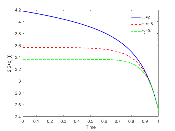
Figure 1: The major agent’s mean reversion rate $2.5+q_{0}(t)$ for various values of $\sigma_{0}$ for the case where $\delta=\delta_{0}=\sigma=1$.

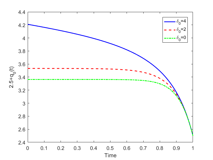
Figure 2: The major agent’s mean reversion rate $2.5+q_{0}(t)$ for various values of $\delta_{0}$ for the case where $\delta=\sigma=\sigma_{0}=1$.

Figures 4 and 4 show the impact of an increase in a representative minor agent’s volatility and degree of risk aversion on the major agent’s mean reversion rate. We observe that this rate decreases slightly with the volatility and the degree of risk aversion of the minor agents. This behavior is due to the structure of (167), which shows that the reversion rate of the major agent depends on that of the minor agents, which, in turn, depends on their parameter values $\sigma$ and $\delta$, as shown in (169).

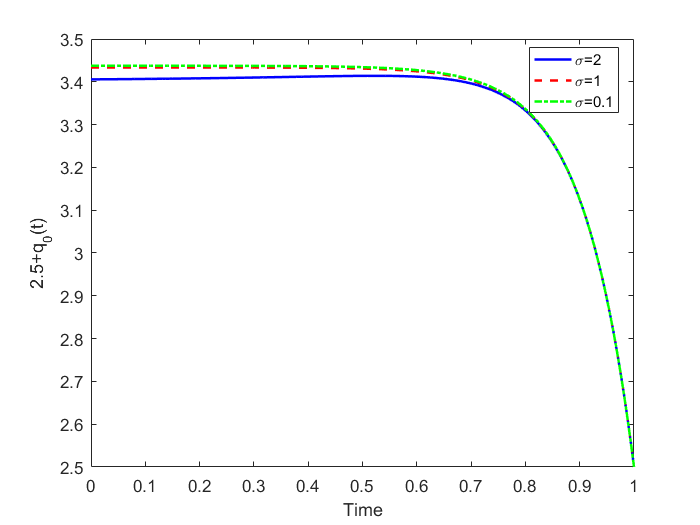
Figure 3: The major agent’s mean reversion rate $2.5+q_{0}(t)$ for various values of $\sigma$ for the case where $\delta=\delta_{0}=\sigma_{0}=1$.

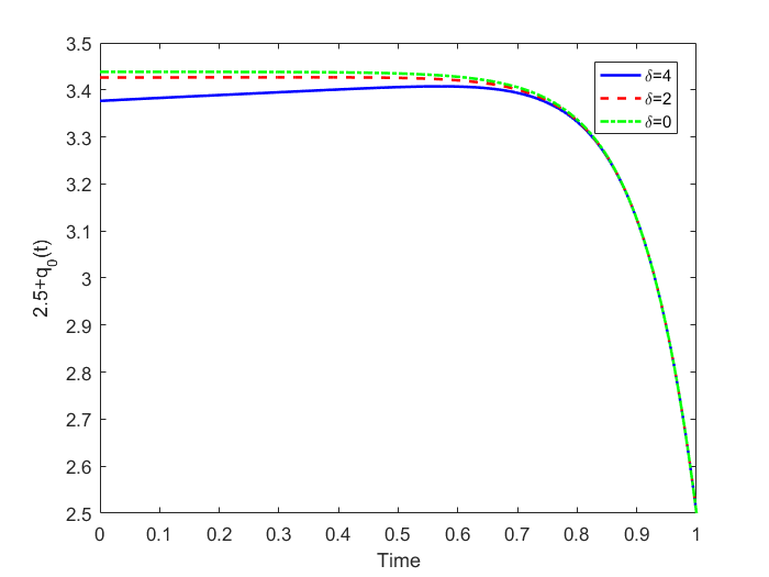
Figure 4: The major agent’s mean reversion rate $2.5+q_{0}(t)$ for various values of $\delta$ for the case where $\delta_{0}=\sigma=\sigma_{0}=1$.

Figures 6 and 6 illustrate how the mean reversion rate of minor agents changes with their volatility and degree of risk aversion. These figures show that the behavior of a representative minor agent follows a similar pattern as that of the major agent, i.e., the mean reversion rate increases with volatility and degree of risk aversion. Furthermore, as depicted in Figure 7, it is evident that the impact of the major agent’s volatility $\sigma_{0}$ on the mean reversion rate of a minor agent is more pronounced, as compared to the opposite scenario illustrated in Figure 4. This observation is intuitively reasonable given the substantial influence of the major agent on the minor agent. Mathematically, this effect can be explained by the explicit presence of $\sigma_{0}$ in equation (169).

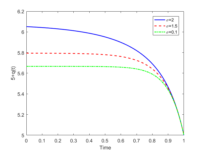
Figure 5: The representative minor agent’s mean reversion rate $5+q(t)$ for various values of $\sigma$ for the case where $\delta_{0}=\delta=\sigma_{0}=1$.

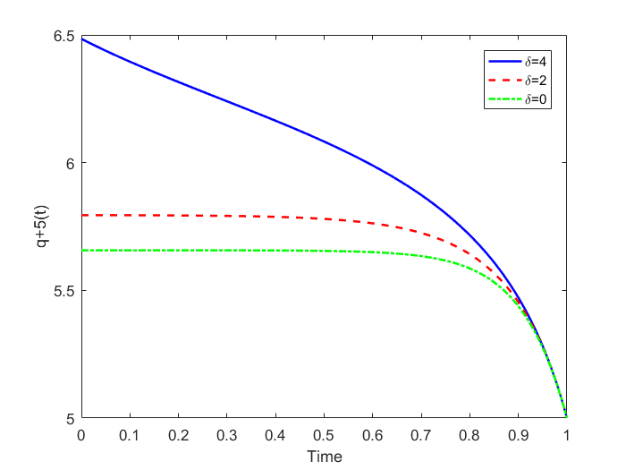
Figure 6: The representative minor agent’s mean reversion rate $5+q(t)$ for various values of $\delta$ for the case where $\delta_{0}=\sigma=\sigma_{0}=1$.

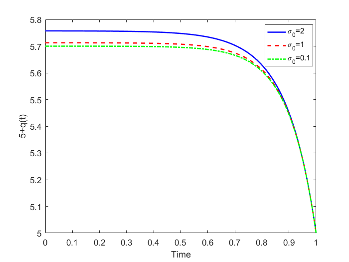
Figure 7: The representative minor agent’s mean reversion rate $5+q(t)$ for various values of $\sigma$ for the case where $\delta_{0}=\sigma=\sigma=1$.

6 Conclusions

In this paper, we began by developing a variational analysis framework for solving risk-sensitive optimal control problems. Subsequently, we extended our investigation to risk-sensitive MFGs that involve both a major agent and a substantial number of minor agents. In particular, we derive an $\epsilon$-Nash equilibrium for LQG models, incorporating risk sensitivity through exponential-of-integral-cost formulations. The variational analysis developed in this work is applied to obtain the equilibrium strategies. Our study emphasizes the significance of incorporating risk sensitivity, particularly in economic and financial models. The obtained results contribute to a deeper understanding of the implications of risk-sensitive decision-making.

References

• Jacobson [1973] D. Jacobson, Optimal stochastic linear systems with exponential performance criteria and their relation to deterministic differential games, IEEE Transactions on Automatic control 18 (1973) 124–131.
• Kumar and Van Schuppen [1981] P. Kumar, J. Van Schuppen, On the optimal control of stochastic systems with an exponential-of-integral performance index, Journal of mathematical analysis and applications 80 (1981) 312–332.
• Nagai [1996] H. Nagai, Bellman equations of risk-sensitive control, SIAM journal on control and optimization 34 (1996) 74–101.
• Pan and Başar [1996] Z. Pan, T. Başar, Model simplification and optimal control of stochastic singularly perturbed systems under exponentiated quadratic cost, SIAM Journal on Control and Optimization 34 (1996) 1734–1766.
• Duncan [2013] T. E. Duncan, Linear-exponential-quadratic gaussian control, IEEE Transactions on Automatic Control 58 (2013) 2910–2911.
• Lim and Zhou [2005] A. E. Lim, X. Y. Zhou, A new risk-sensitive maximum principle, IEEE transactions on automatic control 50 (2005) 958–966.
• Başar [2021] T. Başar, Robust designs through risk sensitivity: An overview, Journal of Systems Science and Complexity 34 (2021) 1634–1665.
• Lasry and Lions [2007] J.-M. Lasry, P.-L. Lions, Mean field games, Japanese journal of mathematics 2 (2007) 229–260.
• Caines [2021] P. E. Caines, Mean field games, in: Encyclopedia of Systems and Control, Springer, 2021, pp. 1197–1202.
• Carmona et al. [2018] R. Carmona, F. Delarue, et al., Probabilistic theory of mean field games with applications I-II, Springer, 2018.
• Bensoussan et al. [2013] A. Bensoussan, J. Frehse, P. Yam, et al., Mean field games and mean field type control theory, volume 101, Springer, 2013.
• Carmona et al. [2015] R. Carmona, J.-P. Fouque, Mousavi, L.-H. Sun, Mean field games and systemic risk, Communications in Mathematical Sciences 13 (2015) 911–933.
• Cardaliaguet et al. [2019] P. Cardaliaguet, F. Delarue, J.-M. Lasry, P.-L. Lions, The master equation and the convergence problem in mean field games:(ams-201), Princeton University Press, 2019.
• Huang [2010] M. Huang, Large-population LQG games involving a major player: the certainty equivalence principle, SIAM Journal on Control and Optimization 48 (2010) 3318–3353.
• Firoozi et al. [2020] D. Firoozi, S. Jaimungal, P. E. Caines, Convex analysis for LQG systems with applications to major–minor LQG mean–field game systems, Systems & Control Letters 142 (2020) 104734.
• Carmona and Zhu [2016] R. Carmona, X. Zhu, A probabilistic approach to mean field games with major and minor players, The Annals of Applied Probability 26 (2016) 1535–1580.
• Garnier et al. [2013] J. Garnier, G. Papanicolaou, T.-W. Yang, Large deviations for a mean field model of systemic risk, SIAM Journal on Financial Mathematics 4 (2013) 151–184.
• Bo and Capponi [2015] L. Bo, A. Capponi, Systemic risk in interbanking networks, SIAM Journal on Financial Mathematics 6 (2015) 386–424.
• Casgrain and Jaimungal [2020] P. Casgrain, S. Jaimungal, Mean‐field games with differing beliefs for algorithmic trading, Mathematical Finance 30 (2020) 995–1034.
• Firoozi and Caines [2017] D. Firoozi, P. E. Caines, The execution problem in finance with major and minor traders: A mean field game formulation, in: Annals of the International Society of Dynamic Games (ISDG): Advances in Dynamic and Mean Field Games, volume 15, Birkhäuser Basel, 2017, pp. 107–130.
• Cardaliaguet and Lehalle [2018] P. Cardaliaguet, C.-A. Lehalle, Mean field game of controls and an application to trade crowding, Mathematics and Financial Economics 12 (2018) 335–363.
• Carmona and Lacker [2015] R. Carmona, D. Lacker, A probabilistic weak formulation of mean field games and applications, The Annals of Applied Probability 25 (2015) 1189–1231.
• Huang et al. [2019] X. Huang, S. Jaimungal, M. Nourian, Mean-field game strategies for optimal execution, Applied Mathematical Finance 26 (2019) 153–185.
• Li et al. [2023] Z. Li, A. M. Reppen, R. Sircar, A mean field games model for cryptocurrency mining, Management Science (2023).
• Lehalle and Mouzouni [2019] C.-A. Lehalle, C. Mouzouni, A mean field game of portfolio trading and its consequences on perceived correlations, arXiv preprint arXiv:1902.09606 (2019).
• Shrivats et al. [2022] A. V. Shrivats, D. Firoozi, S. Jaimungal, A mean-field game approach to equilibrium pricing in solar renewable energy certificate markets, Mathematical Finance 32 (2022) 779–824.
• Gomes and Saúde [2021] D. Gomes, J. Saúde, A mean-field game approach to price formation in electricity markets, Dynamic Games and Applications 11 (2021) 29–53.
• Fujii and Takahashi [2022] M. Fujii, A. Takahashi, A mean field game approach to equilibrium pricing with market clearing condition, SIAM Journal on Control and Optimization 60 (2022) 259–279.
• Shrivats et al. [2021] A. Shrivats, D. Firoozi, S. Jaimungal, Principal agent mean field games in REC markets, arXiv preprint arXiv:2112.11963 (2021).
• Bielecki et al. [2000] T. R. Bielecki, S. R. Pliska, M. Sherris, Risk sensitive asset allocation, Journal of Economic Dynamics and Control 24 (2000) 1145–1177.
• Bielecki and Pliska [2003] T. R. Bielecki, S. R. Pliska, Economic properties of the risk sensitive criterion for portfolio management, Review of Accounting and Finance (2003).
• Fleming and Sheu [2000] W. H. Fleming, S. Sheu, Risk-sensitive control and an optimal investment model, Mathematical Finance 10 (2000) 197–213.
• Tembine et al. [2013] H. Tembine, Q. Zhu, T. Başar, Risk-sensitive mean-field games, IEEE Transactions on Automatic Control 59 (2013) 835–850.
• Saldi et al. [2018] N. Saldi, T. Basar, M. Raginsky, Discrete-time risk-sensitive mean-field games, arXiv preprint arXiv:1808.03929 (2018).
• Saldi et al. [2022] N. Saldi, T. Başar, M. Raginsky, Partially observed discrete-time risk-sensitive mean field games, Dynamic Games and Applications (2022) 1–32.
• Moon and Başar [2016] J. Moon, T. Başar, Linear quadratic risk-sensitive and robust mean field games, IEEE Transactions on Automatic Control 62 (2016) 1062–1077.
• Moon and Başar [2019] J. Moon, T. Başar, Risk-sensitive mean field games via the stochastic maximum principle, Dynamic Games and Applications 9 (2019) 1100–1125.
• Chen, Yan et al. [2023] Chen, Yan, Li, Tao, Xin, Zhixian, Risk-sensitive mean field games with major and minor players, ESAIM: COCV 29 (2023).
• Whittle [1981] P. Whittle, Risk-sensitive linear/quadratic/gaussian control, Advances in Applied Probability 13 (1981) 764–777.
• Duncan [2015] T. E. Duncan, Linear exponential quadratic stochastic differential games, IEEE Transactions on Automatic Control 61 (2015) 2550–2552.
• Huang et al. [2006] M. Huang, R. P. Malhamé, P. E. Caines, Large population stochastic dynamic games: Closed-loop McKean-Vlasov systems and the Nash certainty equivalence principle, Communications in Information & Systems 6 (2006) 221–252.
• Huang and Huang [2017] J. Huang, M. Huang, Robust mean field linear-quadratic-gaussian games with unknown $L^{2}$-disturbance, SIAM Journal on Control and Optimization 55 (2017) 2811–2840.
• Huang and Jaimungal [2017] X. Huang, S. Jaimungal, Robust stochastic games and systemic risk, SSRN preprint: SSRN 3024021 (2017).
• Tchuendom et al. [2019] R. F. Tchuendom, R. Malhamé, P. Caines, A quantilized mean field game approach to energy pricing with application to fleets of plug-in electric vehicles, 2019 IEEE 58th conference on decision and control (CDC) (2019) 299–304.
• Nourian and Caines [2013] M. Nourian, P. E. Caines, $\epsilon$-Nash mean field game theory for nonlinear stochastic dynamical systems with major and minor agents, SIAM Journal on Control and Optimization 51 (2013) 3302–3331.
• Carmona and Wang [2017] R. Carmona, P. Wang, An alternative approach to mean field game with major and minor players, and applications to herders impacts, Applied Mathematics & Optimization 76 (2017) 5–27.
• Huang and Yang [2019] M. Huang, X. Yang, Linear quadratic mean field social optimization: asymptotic solvability, in: 2019 IEEE 58th Conference on Decision and Control (CDC), IEEE, 2019, pp. 8210–8215.
• Lasry and Lions [2018] J.-M. Lasry, P.-L. Lions, Mean-field games with a major player, Comptes Rendus Mathematique 356 (2018) 886–890.
• Huang [2021] M. Huang, Linear-quadratic mean field games with a major player: Nash certainty equivalence versus master equations, Communications in Information and Systems, vol. 21, no. 3 (2021).
• Firoozi [2022] D. Firoozi, LQG mean field games with a major agent: Nash certainty equivalence versus probabilistic approach, Automatica 146 (2022) 110559.
• Bensoussan et al. [2017] A. Bensoussan, M. H. M. Chau, Y. Lai, S. C. P. Yam, Linear-quadratic mean field Stackelberg games with state and control delays, SIAM Journal on Control and Optimization 55 (2017) 2748–2781.
• Moon and Başar [2018] J. Moon, T. Başar, Linear quadratic mean field stackelberg differential games, Automatica 97 (2018) 200–213.
• Ciarlet [2013] P. G. Ciarlet, Linear and nonlinear functional analysis with applications, volume 130, SIAM, 2013.
• Yong and Zhou [1999] J. Yong, X. Y. Zhou, Stochastic controls: Hamiltonian systems and HJB equations, volume 43, Springer Science & Business Media, 1999.
• Chung and Williams [1990] K. L. Chung, R. J. Williams, Introduction to stochastic integration, volume 2, Springer, 1990.
• Karatzas and Shreve [1991] I. Karatzas, S. E. Shreve, Brownian motion and stochastic calculus, volume 113, Springer Science & Business Media, 1991.
• Behr et al. [2019] M. Behr, P. Benner, J. Heiland, Solution formulas for differential sylvester and lyapunov equations, Calcolo 56 (2019) 51.
• Caines and Kizilkale [2017] P. E. Caines, A. C. Kizilkale, $\epsilon$-Nash equilibria for partially observed LQG mean field games with major player, IEEE Transaction on Automatic Control 62 (2017) 3225–3234.
• Moon et al. [2018] J. Moon, T. E. Duncan, T. Başar, Risk-sensitive zero-sum differential games, IEEE Transactions on Automatic Control 64 (2018) 1503–1518.
• Başar and Olsder [1998] T. Başar, G. J. Olsder, Dynamic noncooperative game theory, SIAM, 1998.
• Chang et al. [2022] Y. Chang, D. Firoozi, D. Benatia, Large banks and systemic risk: Insights from a mean-field game model, arXiv preprint arXiv:2305.17830 (2022).