Private and Collaborative Kaplan-Meier Estimators

Abstract.

Kaplan-Meier estimators capture the survival behavior of a cohort. They are one of the key statistics in survival analysis. As with any estimator, they become more accurate in presence of larger datasets. This motivates multiple data holders to share their data in order to calculate a more accurate Kaplan-Meier estimator. However, these survival datasets often contain sensitive information of individuals and it is the responsibility of the data holders to protect their data, thus a naive sharing of data is often not viable.

In this work, we propose two novel differentially private schemes that are facilitated by our novel synthetic dataset generation method. Based on these scheme we propose various paths that allow a joint estimation of the Kaplan-Meier curves with strict privacy guarantees.

Our contribution includes a taxonomy of methods for this task and an extensive experimental exploration and evaluation based on this structure. We show that we can construct a joint, global Kaplan-Meier estimator which satisfies very tight privacy guarantees and with no statistically-significant utility loss compared to the non-private centralized setting.

1. Introduction

Survival analysis or time-to-event analysis (Kleinbaum et al., 2012) refers to all the methods that return statistics on the survival properties of a population. Survival analysis can be utilized in, for example, medical studies to predict the time of death of patients(Goldhirsch et al., 1989; Brenner, 2002), in financial domain to model the time of default of customers or time of unsubscribing from a service (Baesens et al., 2005; Dirick et al., 2017; Lu, 2002) and in general whenever the behavior of a population against time for a specific event of interest should be studied.

One of the mostly-reported, and preferred statistics in survival analysis is the Kaplan-Meier estimator (Goel et al., 2010). This non-parametric estimator uses the survival data to directly approximate the probability of survival for a given population. In the medical domain, this is a very powerful tool, since the effect of, for example, a specific treatment or marker on the overall survival behavior of a population can directly be studied without any complicated formulation or assumptions on the underlying random processes.

The effectiveness and precision of Kaplan-Meier estimators to model the true survival probability can be maximized when they are constructed from a large dataset. Unfortunately, in real world, access to a large and representative dataset is not always possible for individual data centers and research institutes. This motivates collaboration schemes among multiple data holders to jointly build a richer estimator.

Despite this incentive for collaboration, data protection regulations such as General Data Protection Regulation (GDPR) (GDP, 2016), make naive approaches infeasible. Raw data may not simply be shared with other centers and is subject to strict regulations (SUP, 2022; GDP, 2016) to protect the privacy of data contributors, e.g., patients.

Attempts to address the security concerns with making a collaborative Kaplan-Meier estimator, have so far only utilized secure aggregation and encryption schemes (Froelicher et al., 2021; Vogelsang et al., 2020; von Maltitz et al., 2021; Xi et al., 2022). However, these methods increase the computational cost and the execution time and do not scale well to large number of collaborators. Another issue is that these methods cannot offer any privacy guarantees for the released global model. An adversary with access to aggregated statistics can still carry out attacks such as re-identification (El Emam et al., 2011; Rocher et al., 2019) or inference (Backes et al., 2016; Homer et al., 2008).

A solution which theoretically guarantees the privacy of individuals whose data is present in a dataset, is differential privacy(Dwork and Roth, 2014). Differential privacy, which is basically a controlled randomization process, can be applied through different mechanism and at different stages, for example, on data, on functions of data or on aggregated statistics. This randomness ensures the privacy of individuals, however, summary statistics still can be inferred from the dataset. An interesting property of differential privacy is that an adversary, with access to any auxiliary information, is not able to infer further information on any modification of a differentially private state. This is known as the post-processing property of differential privacy.

The studies that attempt to combine differential privacy and Kaplan-Meier estimators have been very limited so far (Gondara and Wang, 2020) and focus on protecting the count numbers and do not propose any solution for when we do not have access to count numbers at each time. The previous method also does not offer protection for the specific times of events. Up until now, no work has suggested differentially private methods that can facilitate a collaboration for this problem.

In this work, we first introduce two new differentially private methods that can be applied on different functions of survival data and based on our methods we suggest various paths that collaborators can take to privately build a joint global Kaplan-Meier estimator. Our paths offer great flexibility for the preferred shared information in a collaborative system and are easy to apply and fast to compute. In summary:

• We present the first approach to the problem of privacy-preserving joint survival estimation over an aggregate of participants and provide a systematic analysis how to achieve this global model.

• We propose two differentially private methods that local sites can utilize for the privacy of their data. We then propose multiple paths that the local site can propagate their private information through, in order to construct a final joint KM estimator. We are able to achieve good utility compared to the centralized setting at a high privacy level ($\varepsilon=1$).

• We are able to release local differentially private surrogate datasets which enable us to construct an accurate, private and joint Kaplan-Meier estimator by pooling these private datasets.

The structure of our paper is as follows: we start off by a brief introduction on survival analysis and also foundations of differential privacy in Section 2, we then give a mathematical presentation of our differentially private methods in Section 3. In Section 4, we explain the private collaboration setting and all the various paths that can be taken by individual collaborators to contribute to a joint global model. We then move to our experiments in Section 5. We first study the effect of hyperparameters in Section 5.4, then we show that our surrogate dataset generation method is stable and accurate in Section 5.3, then show the performance of all our differentially private methods in Section 5.5 and finally and most importantly we show the results for all our private and collaborative paths in Section 5.6. We then give a summary of the related previous work in Section 6 and finally conclude our work in Section 7.

2. Background

In this section, we explain the concepts necessary to understand our methods and the experiments. We first start by introducing the survival probability function and the Kaplan-Meier (KM) estimator for it for the real-world case where number of data is finite and times are discrete. We then introduce a closely-related function over the whole population, namely the event probability mass function.

Finally we move to differential privacy (DP), which is a mathematically driven privacy-preserving method. We will later use DP on various survival statistics to be able to eventually share the survival information in a collaborative system with other participants.

2.1. Survival Analysis and Kaplan-Meier (KM) Estimators

Survival analysis is the collection of statistical methods that aim to model and predict the time duration to an event of interest for a set of data points. As an example, the events of interest in medical survival analysis might be the time it takes for a patient to die from an initial point when the patient enters a study, the time to metastasis, time to relapse, etc.

The dataset for survival analysis is in the form of $D=\{t^{i},e^{i}\}_{i=1}^{N}$ where $t^{i}$ is the time of event for data point $i$ and $e^{i}\in\{0,...,E\}$ is the corresponding type of event for data point $i$, when $E$ types of so-called competing events are considered. In this paper, we focus on single-event survival analysis. In this case, the datapoints might still experience what is known as right-censoring. This happens when an individual is excluded from the study usually due to reasons other than events of interest, or when the event of interest does not occur till the maximum time of the study $T_{\max}$. We consider $e^{i}=0$ when censoring happens, and otherwise; $e^{i}=1$.

The survival function at time $t$ is defined as the probability of the event of interest $t^{*}$ happening after $t$:

(1) $$S(t)=\text{Pr}(t^{*}>t)$$

The survival function is a smooth non-increasing curve over time and its value is bound to $[0,1]$. However, in practice, to model the survival function based on a dataset with finite number of data points, we need to estimate the true value of $S(t)$. The Kaplan-Meier (KM) estimator (Kaplan and Meier, 1958) $\hat{S}$ is a non-parametric step function of data, used to estimate the survival function:

(2) $$\hat{S}(t)=\prod_{t^{\prime}\leq t}\frac{r_{t^{\prime}}-d_{t^{\prime}}}{r_{t^{\prime}}}$$

where $r_{t}$ is the number of datapoints at risk or more commonly known as the risk set (those that have not experienced any type of event) at time $t$ and $d_{t}$ is the number of data points experiencing the event of interest (i.e. $e=1$) at time $t$. Here, we assume that there are $T$ distinct times of event in the whole dataset: $t^{\prime}\in\{0=t_{0},t_{1},t_{2},...,t_{T-1}=T_{\max}\}$. In practice, we can discretize the times of events with an equidistant grid with bin size $b$ and calculate the $\hat{S}(t)$ based on the number of events that occur within each grid

2.2. Event Probability Mass Function

As evident by Equations 1 and 2, the Kaplan-Meier function estimates the probability of the event up to a certain point in time. This is a restrictive view and we might want to instead measure the probability at each specific time or time interval. For this reason, we also consider the closely-related concept of probability mass function:

(3) $$y(t)=\text{Pr}(t^{*}=t|d)$$

which represents the probability that a new data point $d$ will experience the event at time $t$. Throughout this paper, we use probability mass function and probability function or simply probability, interchangeably. The true probability for discretized times of events, $t\in\{0,t_{1},...,T_{\max}\}$, can be approximated by an estimator (Lee et al., 2018; Kvamme et al., 2019) $\hat{y}$:

(4) $$\hat{y}(t_{j})=\begin{cases}0&t_{j}=0\\ \hat{S}(t_{j-1})-\hat{S}(t_{j})&t_{1}\leq t_{j}\leq T_{\max}\\ 1-\sum_{t^{\prime}\leq T_{\max}}y(t^{\prime})&t_{j}=T_{\max}+1\end{cases}$$

(5) $$\hat{S}(t_{j})=1-\sum_{t^{\prime}\leq t_{j}}\hat{y}(t^{\prime})$$

The probability mass function estimator $\hat{y}$ shows the overall probability of incident during each time interval and it contains one element more than $\hat{S}(t)$. This extra element $\hat{y}(T_{\max}+1)$ is considered to capture the probability of event happening past the end time of the study (Kvamme and Borgan, 2021). With this extra element the sum of all the elements in the $\hat{y}$ vector should be 1.0 (i.e. $\sum_{t_{j}=0}^{T_{\max}+1}\hat{y}(t_{j})=1$) as is expected from a probability mass function. As we can see from Equations 4 and 5, the conversion between the estimator for probability mass function $\hat{y}$, and the Kaplan-Meier estimator $\hat{S}$ is straightforward and fast. This gives us the opportunity to convert between the two when we need a different viewpoint on the survival status of the population.

To better demonstrate the relationship between these functions, we provide a toy example in Figure 1 for a small dataset of only 5 individuals. Here $t\in\{0,1,2,3,4,5\}$ months and 2 individuals are censored at times $t=3$ and $t=5=T_{\max}$ (shown with red circles on the survival plot). At each step $t$ we have $\hat{S}(t)=\hat{S}(t-1)\times\frac{r_{t}-d_{t}}{r_{t}}$. Notice that the value of the survival function does not change when a point is censored, however, the individuals that are censored are not considered in the risk set of the next time step. With the same reasoning, the censored data also does not affect the value of the probability function, as seen in, for example, $\hat{y}(3)$. Indeed, the probability mass function only models the probability of the events of interest happening at each time step.

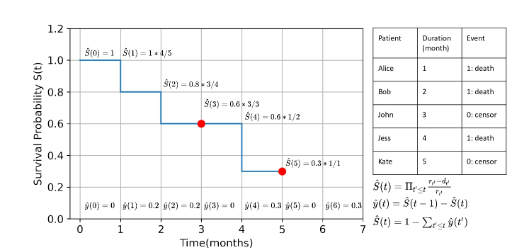
Figure 1. A simple illustrative example of Kaplan-Meier and probability estimators for a dataset of 5 individuals over a time period of 5 months.

2.3. Differential Privacy (DP)

The goal of this paper is to build a global survival model over the collection of data from multiple data owners. However, this collaboration now carries the risk of privacy leakage through these shared data or shared statistics of the data. Differential privacy (Dwork and Roth, 2014) is the standard method to mathematically restrict the probability of information leakage from the data or a function of the data. Differential privacy adds calibrated randomness to data or its functions such that general statistics inferred from the dataset remain accurate but the sensitive information of individual data points is suppressed. There will always be a privacy-utility trade-off: the more randomness is added, the more private the algorithm and less accurate the statistics learned from the collection of the data, and vice versa. Thus we always strive to find an operating point which offers the best privacy-utility trade-off.

Definition 0 ($\varepsilon$-Differential Privacy (Dwork and Roth, 2014)).

A randomized algorithm $\mathcal{A}$ is $\varepsilon$-differentially private, if for any two neighboring datasets $D$ and $D^{\prime}$ differing by at most one data point, and for any $S\subseteq\mathit{Range}(\mathcal{A})$ we have:

$$\Pr(\mathcal{A}(D)\in S)\leq e^{\varepsilon}\Pr(\mathcal{A}(D^{\prime})\in S)$$

Intuitively, this guarantees that an adversary, provided with the output of $\mathcal{A}$, can draw almost the same conclusion (up to ${\varepsilon}$ about whether dataset $D$ or $D^{\prime}$ was used. That is, for any record owner, a privacy breach is unlikely to be due to its participation in the dataset.

2.3.1. Laplace Mechanism

As explained in Definition 1, a randomization process is necessary for differential privacy. There are many mechanism that can be applied on data or functions of data to make these differentially private. Here we focus on the so-called Laplace mechanism. But we first need to define the global sensitivity of a function (Dwork and Roth, 2014):

Definition 0 (Global $L_{p}$-sensitivity).

For any function $f:\mathcal{D}\rightarrow\mathbb{R}^{k}$, the $L_{p}$-sensitivity of $f$ is $\Delta_{p}f=\max_{D,D^{\prime}}||f(D)-f(D^{\prime})||_{p}$, for all $D,D^{\prime}$ differing in at most one record, where $||\cdot||_{p}$ denotes the $L_{p}$-norm.

The Laplace Mechanism (Dwork and Roth, 2014) consists of adding Laplace noise to the true output of a function, in order to make the function differentially private.

Definition 0 (Laplace Mechanism (Dwork and Roth, 2014)).

For any function $f:\mathcal{D}\rightarrow\mathbb{R}^{k}$, the randomized function $\mathcal{A}$:

$$\mathcal{A}(f(.),\varepsilon)=f+(\mathcal{L}_{1},...,\mathcal{L}_{k})$$

is differentially private. Where $\mathcal{L}_{i}$ are drawn independently and randomly from a Laplace distribution centered at 0, with $\mathsf{pdf}_{\mathcal{L}(0,l)}(x)=\frac{1}{2l}\exp\left(-\frac{\lvert x\rvert}{l}\right)$ where the scale parameter $l$ is dependant on the sensitivity through $l=\frac{\Delta_{1}f}{\varepsilon}$.

Differential privacy is immune to post-processing (closure under post-processing), this means that an adversary cannot compute a function of the output of a differentially private mechanism $\mathcal{A}$ and make it less differentially private.

Theorem 4 (Post-Processing Property (Dwork and Roth, 2014)).

Let $\mathcal{A}$ be an $\varepsilon-$DP privacy mechanism which assigns a value $\mathit{Range}(\mathcal{A})$ to a dataset $D$. Let $\mathcal{B}$ be an arbitrary randomized mapping which takes as input $O\in\mathit{Range}(\mathcal{A})$ and returns $O^{\prime}\in\mathit{Range}(\mathcal{B})$. Then $\mathcal{B}\circ\mathcal{A}$ is also $\varepsilon$-differentially private.

3. Differentially Private Survival Statistics Estimators

In this section, we explain the methods that can be used to make a survival dataset or its functions differentially private. Based on these methods, we can later build paths that enable a collaborative learning system. We will first review a previously-suggested method -which we call DP-Matrix- that perturbs the matrix of count numbers at each unique time of event. We then introduce our two novel methods, DP-Surv and DP-Prob, which are more flexible and can be applied directly on Kaplan-Meier function and probability estimator, respectively. In the end of this section, we make a comparison of the methods and argue why our DP-Surv and DP-Prob offer better privacy compared to DP-Matrix.

3.1. DP-Matrix

The first method we look at, applies DP directly on the number counts $d_{t_{j}}$ and risk set $r_{t_{j}}$ in the dataset. In this method suggested by (Gondara and Wang, 2020), first a partial matrix $M=[r_{0},d_{0},d_{t_{1}},...,d_{T_{\max}}]$ of number of events at each unique incident time $d_{t_{j}}$ and the total number of individuals at the initial time $r_{0}$ is constructed, then Laplace noise with sensitivity of 2 is directly added to these numbers, i.e:

(6)

where $M^{\prime}$ is now the DP partial matrix. The authors use this sensitivity since adding or removing one datapoint from the dataset will at most change the count number by 2 (simultaneously in $r_{0}$ and $d_{t_{j}}$ values). After obtaining the noisy $d^{\prime}_{t_{j}}$ values and the noisy number of individuals at the start of the study $r^{\prime}_{0}$, the remaining number of at risk is calculated by:

(7) $$r^{\prime}_{t_{j}}=r^{\prime}_{t_{j-1}}-d^{\prime}_{t_{j-1}}\qquad\forall t_{j}\in\{t_{1},...,T_{\max}\}$$

We can also modify this algorithm to include censored data. So the partial matrix will be $M=[r_{0},d_{0},c_{0},d_{t_{1}},c_{t_{1}},....,d_{T_{\max}},c_{T_{\max}}]$ where $c_{t_{j}}$ is the number of censored individuals at unique time of incident $t_{j}$. The Laplace noise is then added to these numbers to form the DP partial matrix $M^{\prime}$. The noisy risk set at different times will then be calculated as:

(8) $$r^{\prime}_{t_{j}}=r^{\prime}_{t_{j-1}}-(d^{\prime}_{t_{j-1}}+c^{\prime}_{t_{j-1}})\qquad\forall t_{j}\in\{t_{1},...,T_{\max}\}$$

We call this method differentially private matrix or DP-Matrix for short.

A major point of consideration when working with DP-Matrix is that it only perturbs the count numbers at distinct recorded times of events. This means that the algorithm would not perturb the times of incident, hence the times of the events are not protected by this method and this still poses privacy concerns for the dataset. To tackle this problem, we use the KM estimator and the probability estimator sampled at equidistant time intervals as the functions that are to be perturbed by DP mechanism. In the following, we will present our proposed approaches that address this issue.

3.2. DP-Surv

In our first proposed method we strive to offer more flexibility with respect to the function that differential privacy is applied on. This method that we call differentially private Kaplan-Meier estimator or DP-Surv for short, directly tweaks the Kaplan-Meier survival estimator to make it private and no access to the dataset is needed. We also address the issue of privacy of times of events (as discussed in Section 3.1) by sampling the KM estimator at equidistant time intervals. By doing so, the function no longer contains the sensitive distinct times of events and applying differential privacy on this vector now also protects times.

Consider $\hat{S}(t)$ the vector of survival estimates containing the sampled values of the continuous KM function at equidistant time intervals. If we have a bound on its $L_{1}$ sensitivity, we can use the Laplace mechanism (Definition  3) to make this vector differentially private.

Theorem 1.

The $L_{1}$ sensitivity of $\hat{S}(t)$ for datasets with no censored data is $\Delta_{1}\hat{S}=\frac{{T-1}}{N}$ and for datasets with censored data is $\Delta_{1}\hat{S}=\frac{{T}(1+C)}{N}$, where $N$ and $C$ are the total number of data points and the total number of censored data points in the dataset, respectively. $T$ is the number of time bins in the equidistant grid over $t=0$ till $t=T_{\max}$.

Proof.

We provide the proof for $L_{1}$ sensitivity of the Kaplan-Meier estimator $\hat{S}(t)$, in Appendix A. ∎

We see that the sensitivity grows proportional to the number of time intervals $T$ for both cases. This means that only if $T\ll N$ (or $T+TC\ll N$ for when $C\neq 0)$, the sensitivity is reasonably small, otherwise, the DP noise will destroy the utility. Inspired by works of (Rastogi and Nath, 2010; Kerkouche et al., 2021), we solve this issue by first transforming the discrete KM vector with discrete cosine transform (DCT), adding Laplace noise only to the first $k$ coefficients of this vector $DCT(S(t))$ and then transforming the partially-noised vector back to the original time space. The first coefficients of the transformed vector $DCT(S(t))$ only capture the large-scale structure of the KM curve and contain the most condensed statistics such as the mean of the vector. The fine details which are stored in the $T-k$ last coefficients are masked to zero before transforming back to the original space. This helps preserve the overall shape of the KM curve while offering tight privacy guarantees.

Theorem 2.

Denote ${D}^{k}={DCT}^{k}(\hat{S}(t))$ the first $k$ coefficients of the discrete cosine transform of $\hat{S}(t)$, then $\Delta_{1}{D}^{k}\leq\sqrt{k}\Delta_{2}\hat{S}(t)$.

Proof.

DCT preserves the $L_{2}$ norm of vectors, so when taking only the first $k$ coefficients, we have $\Delta_{2}{D}^{k}\leq\Delta_{2}\hat{S}(t)$. And using the inequality between $L_{1}$ and $L_{2}$ norms we have $\Delta_{1}{D}^{k}\leq\sqrt{k}\Delta_{2}{D}^{k}$. ∎

Theorem 3.

The $L_{2}$ sensitivity of $\hat{S}(t)$ for datasets with no censored data is $\Delta_{2}\hat{S}=\frac{\sqrt{T-1}}{N}$ and for datasets with censored data is $\Delta_{2}\hat{S}=\frac{\sqrt{T}(1+C)}{N}$, where $N$ and $C$ are the total number of data points and the total number of censored data points in the dataset, respectively. $T$ is the number of time bins in the equidistant grid over $t=0$ till $t=T_{\max}$.

Proof.

We provide the proof for $L_{2}$ sensitivity of the Kaplan-Meier estimator $\hat{S}(t)$, in Appendix A. ∎

So based on Theorem 2 and the Laplace mechanism 3, we set the scale of the noise that is added to the $k$ first coefficients of $DCT(\hat{S}(t)$ to:

(9) $$l=\frac{\Delta_{1}D^{k}}{\varepsilon}=\frac{\sqrt{k}\Delta_{2}\hat{S}}{\varepsilon}$$

We will then pad this differentially private vector with $T-k$ zeros and transform to the real time space to get a differentially private Kaplan-Meier estimator $\hat{S}^{\prime}(t)$ (for detailed explanation see (Rastogi and Nath, 2010)). Note that the use of an equidistant time grid is necessary for a a meaningful discrete cosine transformation of the survival estimator vector, otherwise the coefficients would not represent details at gradually-growing scales, correctly.

By definition, the Kaplan-Meier estimator should be a non-increasing function. To achieve this, after adding Laplace noise, padding with zeros and transforming back to the real-time space, we apply a post-processing function:

$$p(\hat{S}^{\prime}(t))=\{\forall t>t^{\prime}:(\hat{S}^{\prime}(t)>\hat{S}^{\prime}(t^{\prime}))\rightarrow\texttt{clip}(\hat{S}^{\prime}(t),\hat{S}^{\prime}(t^{\prime}),0)\}$$

where $\texttt{clip}(x,up,low)$ is a clipping function which clips the input $x$, to upper bound $up$ and lower bound $low$. According to the post-processing property of the DP (Theorem 4), the new $\hat{S}^{\prime}$ will also satisfy $\varepsilon$-DP.

3.3. DP-Prob

The next privacy-preserving method that we propose, adds DP randomness to the probability mass function estimator $\hat{y}(t)$. We call this method differentially private probability estimator or DP-Prob for short. Here again, we have the advantage that no direct access to data is required and the probability estimator is modified, directly. We also assume an equidistant time grid when sampling the values of the probability estimator function, to address the issue of privacy of times of events.

Consider $\hat{y}(t)$ the vector of probability estimates containing the sampled values of the continuous probability estimator function at equidistant time intervals. If we have a bound on its $L_{1}$ sensitivity, we can use the Laplace mechanism (Definition  3) to make this vector differentially private.

Theorem 4.

The $L_{1}$ sensitivity of the probability mass function estimator for datasets with no censored data is $\Delta_{1}\hat{y}=\frac{2}{N}$ and for datasets with censored data points, is $\Delta_{1}\hat{y}=\frac{TC}{N}$. where $C$ and $N$ are the total number of censored data and the total number of data points, respectively, and $T$ is the number of time bins in the equidistant grid over $t=0$ till $t=T_{\max}$.

Proof.

We provide the proof for $L_{1}$ and $L_{2}$ sensitivity of the probability mass function estimator $\hat{y}(t)$, in Appendix B. ∎

Here, the adverse effect of $C$ and $T$ on the sensitivity is less compared to $\hat{S}(t)$, especially when no censored data are in the dataset the sensitivity only depends on the total number of datapoints. So, we directly apply the Laplace mechanism 3, with a noise scale of $l=\frac{\Delta_{1}\hat{y}}{\varepsilon}$ to each element of the probability vector. Here, we do not have the non-increasing condition of KM estimators, however, we should make sure that $\hat{y}^{\prime}(t)$ resembles a probability mass function, that is, the values are between 0 and 1, and $\sum_{t=0}^{T+1}\hat{y}^{\prime}(t)=1$. For this reason we apply the following post-processing steps:

$$\hat{y}^{\prime}(t) \leftarrow \texttt{clip}(\hat{y}^{\prime}(t),1,0)\qquad\forall t\in\{1,...,T+1\}$$

$$\hat{y}^{\prime}(t) \leftarrow \frac{\hat{y}^{\prime}(t)}{\sum_{t=0}^{T+1}\hat{y}^{\prime}(t)}\qquad\forall t\in\{1,...,T+1\}$$

Note that the discretized probability estimator function $\hat{y}(t)$ is $(T+1)$-dimensional to account for the probability of events happening after the maximum time of study.

Comparison of the Three DP Methods

There are various advantages to using DP algorithms that modify $\hat{S}$ or $\hat{y}$, directly, as opposed to number counts. In a lot of commonly used packages for survival analysis (e.g. lifelines, pycox , scikit-survival, etc.), the data should be in form of $D=\{t^{i},e^{i}\}_{i=1}^{N}$ and not the number count. This means that for using DP-Matrix we need to convert between survival data and number counts multiple times. Also it is customary for medical centers to only publish survival curves over the whole population as opposed to number counts at each distinct time. This means that the privacy provider might not even have access to the dataset at all. For these reasons, it is important to explore DP methods that can be applied on KM/probability estimators, directly and efficiently. Finally, as mentioned before, DP-Matrix perturbs the number counts at unprotected distinct times of events and suggests no protection mechanism for these times. By reading the values of the $\hat{S}$ and $\hat{y}$ on an equidistant grid and applying DP on these vectors, we also offer protection of the times themselves.

4. Private Kaplan-Meier Estimator Across Multiple Sites

In this section we address the challenge of constructing a reliable and privacy-preserving KM curve over a dataset that is distributed across multiple sites. These sites have an incentive to collaborate to generate the most accurate KM estimator, by taking advantage of the union of their datasets. Privacy protection laws (e.g. Politou et al., 2018; Voigt and Von dem Bussche, 2017; Beverage, 1976; Hodge Jr et al., 1999) and concerns about adversarial attacks (El Emam et al., 2011; Malin, 2005) are some of the barriers that make these collaborators reluctant to share their data or functions of their data - including the KM estimate generated on their data - with each other.

We propose differential privacy (Section 2.3), as a method to protect the privacy of the dataset of each site. We then combine the private information from each site to construct a global estimation for the survival function over all of the data.

We have summarized the overall scheme of our solutions to this problem in the form of a graph in Figure 2. In what follows, we expand on this figure and clarify the possible routes that can be taken to arrive at a final goal of a global and private KM estimator $\hat{S}^{\prime}(t)$. We will first describe the vertical movement in the diagram which corresponds to changing representations of the data. We then move to clarification of the horizontal movement in the graph which corresponds to our various DP methods as suggested in Section3.

Figure 2. Overall scheme of paths that are possible to construct a collaborative private KM estimator over the union of datasets.

4.1. Vertical Movement in the Graph: Representation Conversion

A vertical movement at any of the “stops” in our graph will change the representation of the data. There are many reasons one might want to move along the representations. We take advantage of different representations to add DP noise to different functions of the data, in order to assess the utility of our DP methods for a fixed level of privacy guarantee. We will also explain in the end of this section why a conversion back to a dataset is necessary to calculate the performance metrics for our methods. In the following we will walk through conversion methods between these representations.

Data to Kaplan-Meier estimator:

If a survival dataset is available (the second row from top), the KM estimator can easily be constructed using Equation 2.

Kaplan-Meier estimator to probability estimator and vice versa:

If a KM estimator over a survival dataset is available (the third row from top), using Equation 4, the estimator for the probability mass function can easily be constructed. The conversion in the other way, from probability estimator (the lowest row) is also seamless by utilizing Equation 5. It is worth mentioning that no information is lost when converting between KM estimator and its counterpart, probability estimator, and we can easily convert between these two rows.

Estimators to Data: Surrogate Dataset

Kaplan-Meier estimator (and equally the probability estimator) summarizes the survival information contained in the dataset into one non-parametric curve over time (Kaplan and Meier, 1958; Lee et al., 2018; Kvamme et al., 2019). For meta-analysis or computing more complicated metrics over the population, access to only KM/probability estimator functions is not sufficient and we need the dataset. In our study, one might end up with access to only KM/probability functions (lower two rows) for two reasons: a) when only the KM/probability estimator is shared with other sites, b) when DP is used to modify these two functions. This motivates us to attempt to reconstruct a dataset based on values of probability estimator:

(10) $$\mathcal{R}_{\text{surr}}:[0,1]^{T_{\max}+1}\rightarrow\mathcal{D}$$

where $\mathcal{R}_{\text{surr}}$ is a reconstruction function that takes probability values as input and outputs a surrogate dataset $D_{\text{surr}}\subset\mathcal{D}$.

The problem of converting survival values to the corresponding dataset has been explored in, for example, (Guyot et al., 2012; Wei and Royston, 2017). Here, the most accurate version of the algorithm requires access to various parameters, such as number at risk at regular intervals during the time-frame of the study and total number of events $(\sum_{t_{j}=0}^{T_{\max}}d_{t_{j}})$ over the duration of study. When only the probability estimator or KM estimator are provided, we do not have access to these two parameters, rather the overall probability of experiencing the event at each interval or probability of survival at each interval, respectively. Previous work (Guyot et al., 2012) states that when neither the total number nor multiple values for number at risk are provided, we can assume that there are no censored observations. They mention that although this is a strong assumption, any other assumption about the data without further information would be just as strong.

Inspired by these arguments we propose a simple, yet effective algorithm to construct a surrogate dataset with access to only probability mass function estimator. Algorithm 1 outlines the procedure. We assume that during the time-frame of the study no censoring happens and the probabilities directly reflect the number of datapoints experiencing the event of interest at each time-interval. As explained in Section 2.2, the extra element of the probability vector, $\hat{y}({T_{\max}+1})$, represents the probability of event happening after the maximum time of study $T_{\max}$. So we convert this value to datapoints censored at time $T_{\max}$, as formulated in lines 9-12 of our algorithm.

Since the conversion between the Kaplan-Meier estimator and the probability estimator is straightforward and lossless (see Section 2.2), when access to only KM values is granted, we can first convert to probability values and then apply Algorithm 1 to construct the surrogate dataset.

Algorithm 1
Surrogate Dataset Construction $\mathcal{R}_{\text{surr}}$
Vector of survival probabilities $\hat{y}=\{\hat{y}_{t_{j}}\}_{t_{j}=0}^{T_{\max}+1}$, tuple of datapoints $d^{i}=\{t^{i},e^{i}\}$, number of data points to consider $n$, function to round to the nearest integer $round()$.

1:initialize empty surrogate dataset $D_{\text{surr}}=[]$

2:for $t_{j}=0,...,T_{\max}$ do

3:     $num_{t_{j}}\leftarrow round(\hat{y}_{t_{j}}*n)$

4:     for $i=1,...,num_{t_{j}}$ do

5:         $d^{i}=\{t_{j},1\}$

6:         $D_{\text{surr}}$.append($d^{i}$)

7:     end for

8:end for

9:$num_{T_{\max}+1}\leftarrow round(\hat{y}_{T_{\max}+1}*n)$

10:for $i=1,...,num_{T_{\max}+1}$ do

11:     $d^{i}=\{T_{\max},0\}$

12:     $D_{\text{surr}}$.append($d^{i}$)

13:end for

14:return $D_{\text{surr}}$

Data to Performance Metrics

As explained, when we have access to a real or surrogate dataset (the second row from top) we are much more flexible to run more complex metrics on the population to measure their survival properties. The measurement metrics will be explained in detail in Section 5.2 just before starting our experiments.

4.2. Crossing the Privacy Barrier: DP-methods

In this section, we explain the horizontal movement in our graph across the Privacy Barrier line (leftmost column to the middle column). This is the stage when each site utilizes differential privacy, locally, to construct a private dataset or a private function of their dataset. We look at 3 different DP methods to apply privacy, locally, as explained in Section 3. In the centralized setting, the adversary can be any external entity that has a view on any information that is released from the client’s database. The adversary is passive (i.e., honest-but-curious).

DP-Matrix

When access to the full dataset and the times of events is provided, we can apply DP-Matrix (see Section 3.1) directly on count numbers at each distinct time of event.

DP-Surv

With more flexibility compared to DP-Matrix method, when only access to (discretized) survival functions is provided, each site can directly apply DP-Surv (see Section 3.2) on their survival functions. If the raw dataset is available, first the KM curve is constructed and then this DP method is applied on the KM function. If only probability estimator function is provided, first the corresponding KM estimator is caclulated and then DP is applied.

DP-Prob

When only access to probability mass function is granted, DP is applied according to Section 3.3 to this function. If only the dataset is available, the probability function is first constructed and then the DP noise is added to this vector. Again, when only KM curve is provided the conversion to the probability estimator function is easily possible through Equation 4.

4.3. Crossing the Collaboration Line

We will now continue further in the horizontal direction, from the locally DP functions (middle column) to global, privacy-preserving survival statistics over all of the data (right column). The goal is to collect the privacy-preserving statistics from all sites and construct a KM estimator that uses the information contained in the union of the datasets of all the collaborating sites. A central server is responsible to collect the survival statistics from all site and aggregate them. In the collaborative setting, the adversary can be the central server, other participants or any other entity that has a view on any information released from the clients’ side. The adversary is passive (i.e., honest-but-curious), that is, it follows the protocol faithfully.

As explained in Section 4.1, we always have the option to convert to other representations along the vertical line. So regardless of what method we choose from Section 4.2, the local sites can share one of the 3 different representations of the differentially private information with the central server for a joint calculation of the global model:

Private Data

After applying DP to data directly via DP-Matrix we will be left with a differentially private dataset. However, applying DP-Surv or DP-Prob only changes the KM function and probability function, respectively. To go back to the space of datasets, we can deploy our surrogate data generation method from Section 4.1 to construct a differentially private dataset. Note that since the input of Algorithm 1 is the private probability estimator function, the constructed surrogate dataset will also be private due to the post processing property of DP. For when we choose the DP-Surv method, we can convert the DP KM vector to a DP probability vector first using the Equation 4 and then use the surrogate generation method. Each site can then share their private dataset with the central server and the metrics over the pooled data can be used to construct a global and private KM estimator.

Private KM Estimators

If we choose to convert our DP representations to a private local KM estimator, we can share this estimator with the central server. By inspecting Equation 2, for $K$ collaborating sites we have:

(11) $$\hat{S}_{avg}(t)=\prod_{t^{\prime}\leq t}\left(1-\frac{\sum_{k=1}^{K}d_{t^{\prime},k}}{\sum_{k=1}^{K}r_{t^{\prime},k}}\right)$$

for $t\in\{0,...,T_{\max,k}\}$ distinct times of events in the whole global dataset. We can see that it is mathematically not possible to calculate this average function solely based on the values of the local $\hat{S}^{\prime}(t)$ that are shared, because we need access to the risk sets and number of events at a global level. We propose to estimate this by averaging the local KM estimators:

(12) $$\hat{S}^{\prime}_{avg}(t)=\frac{1}{K}\sum_{k=1}^{K}\hat{S}^{\prime}_{k}(t)$$

The private, global KM estimator can then be used, directly, or converted to its corresponding private surrogate dataset on the server side, to calculate the global metrics.

Private Probability Estimators

The last possible option is to either use DP-Prob directly or to convert our private dataset or private KM estimator - which are obtained by DP-Matrix or DP-Surv, respectively - to a DP probability estimator $\hat{y}^{\prime}$. Unlike $\hat{S}(t)$, each of the local and private $\hat{y}^{\prime}(t)$’s are in form of a probability mass function. In absence of auxiliary information, an effective method to combine probability mass functions is to take the average (Hill and Miller, 2011) over all K sites:

(13) $$\hat{y}^{\prime}_{avg}(t)=\frac{1}{K}\sum_{k=1}^{K}\hat{y}^{\prime}_{k}(t)$$

The private, global probability mass function can then be converted to its corresponding private surrogate dataset or KM estimator to calculate the global metrics on.

5. Experiments

In this section we demonstrate the efficiency of our differentially private methods in a collaborative setting on real-world medical datasets. We first give an overviews of the datasets and then explain the metrics used to evaluate the success of our methods in Section. 5.2. We then show in Section 5.3 that our suggested dataset generation Algorithm 1 is robust and is able to closely mimic the behavior of the original datasets. Next, in Section 5.4 we run experiments that help us tune the hyperparameters of our DP methods. With these found hyperparameters, we initially run the DP methods in a centralized setting in Section 5.5. Finally, we progress to the main goal of our work, to show how our methods and suggested paths according to our workflow (as described in Figure 2 of Section 4) help us to accurately generate a joint and private Kaplan-Meier estimator over multiple data holders.

5.1. Datasets

For our experiments, we chose 3 established publicly-available survival medical dataset:

Rotterdam and German Breast Cancer Study Group (GBSG): Contains data of 2232 breast cancer patients from the Rotterdam tumor bank (Foekens et al., 2000) and the German Breast Cancer Study Group (GBSG) (Schumacher et al., 1994). $960(43\%)$ patients are censored. The data is pre-processed similar to (Katzman et al., 2018) with a maximum survival duration of 87 months.

The Molecular Taxonomy of Breast Cancer International Consortium (METABRIC): This dataset contains gene and protein expressions of 1904 individuals (Curtis et al., 2012). We use a dataset prepared similar to (Katzman et al., 2018). The maximum duration of the study is 355 months ($\sim 30$ years), 801 $(42\%$ of total) patients were right-censored and 1103 $(58\%$ of total) were followed until death.

Study to Understand Prognoses Preferences Outcomes and Risks of Treatment (SUPPORT): This dataset consists of 8873 seriously-ill adults (Knaus et al., 1995). The dataset has a maximum survival time of 2029 days $(\sim 5.6)$ years and $32\%(2839)$ of data is right-censored. We use a pre-processed version according to (Katzman et al., 2018).

Dataset Usage

As explained in Section3, in the most general case, the sensitivity of our differentially private methods DP-Surv and DP-Prob scales proportional to $C$ the number of censored data points in the whole dataset. Previous studies (Ranganathan et al., 2012; Leung et al., 1997; Coemans et al., 2022) mention that the censoring mechanism is unknown in most studies and this introduces bias in the survival behavior of the population. Since the proportion of censored data in all 3 datasets is large ($32\%$-$43\%$) and this will negatively affect the sensitivity of the DP mechanism and also based on the reasoning that these points introduce bias in the outcome, we choose to run all our experiments on only the non-censored ($e=1$) portion of all 3 datasets. For each dataset, we represent the total number of data points, the total number of censored data points and the total number of non-censored data points with $N$, $C$ and $\bar{N}$, respectively.

5.2. Metrics

Logrank Test

In our experiments, we need to compare the quality of DP-generated KM curves and strive for the closest KM distribution to the one generated from the original dataset. To compare KM distributions of two samples, usually hypothesis testing is used. The logrank test is the most common of such tests for survival analysis.

The logrank test (Mantel et al., 1966) is a type of non-parametric hypothesis test used to compare the survival distribution of two populations, even when the right-censored data is present. The null hypothesis for this test is that the two populations have the same survival distribution. So if we calculate a $p-$value smaller than the desired significance level, we reject the null hypothesis and consider the two populations different. However, if the $p-$value is larger than the significance level, we cannot claim anything. In statistics, usually a value of $p<0.05$ is considered small enough to reject the null-hypothesis, however, a lot of debate is surrounding the topic, with many arguing that a much smaller value is needed (Ioannidis, 2019; Di Leo and Sardanelli, 2020).

Consider we would like to compare the survival distribution of two populations $j=\{1,2\}$, and the combined data over these two populations has $t=\{1,...,T\}$ distinct times of event. We define $d_{t,j}$ as observed number of events in group $j$ at time $t$, and $d_{t}=d_{t,1}+d_{t,2}$ as total events at time $t$. If we consider $r_{t,j}$ as the number at risk in group $j$ at time $t$ and $r_{t}=r_{t,1}+r_{t,2}$ as the total number at risk at time $t$, the expected number of events for group $j$ at time $t$ under the null hypothesis would be $E_{t,j}=r_{t,j}\frac{d_{t}}{r_{t}}$.

Using these notations, we can construct test statistics for population 1 under the null hypothesis as:

(14) $$Z=\frac{\sum_{t=1}^{T}(d_{t,1}-E_{t,1})}{\sqrt{\sum_{t=1}^{T}V_{t,1}}}$$

where $V_{t,1}$ is the variance in group 1 at time $t$ and is defined as:

(15) $$V_{t,1} = E_{t,1}(\frac{r_{t}-d_{t}}{r_{t}})(\frac{r_{t}-r_{t,1}}{r_{t}-1})$$

$$= \frac{r_{t,1}r_{t,2}d_{t}(r_{t}-d_{t})}{r_{t}^{2}(r_{t}-1)}$$

By the central limit theorem $Z\sim\mathcal{N}(0,1)$, where $\mathcal{N}(0,1)$ is a Gaussian probability with mean 0 and variance 1. Based on this approximation, the value of $Z$ can be compared with tails of the standard Gaussian distribution in order to obtain the $p-$value of the null hypothesis.

Median Survival Time and Survival Percentage

As mentioned, the $p-$value of the logrank test is a limited metric for comparing survival functions, and we cannot claim anything for large $p-$values. Moreover, the logrank test is defined under the assumption of non-crossing survival curves and it will not correctly represent similarity or dissimilarity for complicated survival functions that cross over each other at some point in time (Bouliotis and Billingham, 2011).

For these reason, other works (e.g. Guyot et al., 2012; Wei and Royston, 2017) also report median survival time and survival percentage at specific time points over the timeframe of each dataset. The median which is the time at which the survival function reaches a value of $\hat{S}=0.5$, is a robust measure over the dataset and gives a general idea about the survival property of the dataset. Another important concept in survival studies is the behavior of the population at the beginning, middle point of the study and towards the end of the study. Therefore we choose to report the survival probability at three different time points $\{0.25T_{\max},0.5T_{\max},0.75T_{\max}\}$, with $T_{\max}$ being the maximum time in the study. For the median and survival probabilities, we can also define confidence interval (systematic error) which is defined directly over the KM curves. The variance of the KM estimator according to Greenwood’s formula (Greenwood et al., 1926) is:

(16) $$\hat{V}(t)=\hat{\sigma}^{2}(t)=\hat{S}^{2}(t)\sum_{t^{\prime}\leq t}\frac{d_{t^{\prime}}}{r_{t^{\prime}}(r_{t^{\prime}}-d_{t^{\prime}})}$$

Once more, for large samples, the Kaplan-Meier curve evaluated at time $t$ is assumed to be normally distributed and the $100(1-\alpha)\%$ confidence interval (CI) can be obtained as:

(17) $$\hat{S}(t)\pm z_{1-\alpha/2}\hat{\sigma}(t)$$

where $z_{1-\alpha/2}$ is the $1-\alpha/2$ fractile of the standard normal distribution. This assumption can be improved for smaller sample size, using Greenwood’s exponential log-log formula (Sawyer, 2003):

(18) $$\hat{S}(t)^{\exp(\pm z_{1-\alpha/2}\hat{\sigma}(t)/[\hat{S}(t)\ln\hat{S}(t)])}$$

For some of our experiments we also introduce a measure of median that makes comparison between different datasets easy. We call this the calibrated median difference or cmd:

(19) $$\text{cmd}_{n,b}=\frac{\mathopen{|}\text{median}_{n,b}-\text{median}_{\text{original}}\mathclose{|}}{\text{median}_{\text{original}}}$$

Privacy Guarantees

According to the post-processing property of DP explained in Section 4, any function of a differentially private function is also differentially private.

In DP-Matrix, we directly add noise to the counts in the original dataset, thus any function of these noisy data, including the constructed $\hat{S},\hat{y}$, as well as the surrogate dataset that helps to calculate logrank test statistics and confidence intervals are differentially private.

For our DP-Surv and DP-Prob methods, any function of these two functions is differentially private and this includes the surrogate dataset used to calculate the test statistics and confidence intervals.

5.3. Construction of Surrogate Datasets

Our metrics (see Section5.2) are reliant on access to individual data points and their times of event in each dataset. This problem motivated us to develop our surrogate dataset generation Algorithm 1 and it is a very important aspect of all of our experiments, since no matter which route we take in Figure 2 of our workflow, we eventually need to reconstruct surrogate datasets to be able to calculate the performance metrics for our methods. In this section, we study the performance of our surrogate dataset generation method in a centralized setting and without any privacy-preserving mechanism.

Parameters

By inspecting Algorithm 1, we see that $n$, the total number of points we choose to populate a KM curve with, is one of the hyperparameters that we need to optimize. We also show in Sections 3.2 and 3.3 that our DP-Surv and DP-Prob methods are based on equidistant time of event discretization. Since we would like to remain consistent among all DP methods, we choose an equidistant grid of size $b$ for times of events for all our experiments from this point on. Now $b$ is also a hyperparameter that can change the results and needs optimization.

Setup

For all our datasets we first produce the discretized KM function $\hat{S}$ and its corresponding probability function $\hat{y}$ based on our bin length $b$, then run our surrogate generation algorithm with $n=\{0.5\bar{N},\bar{N},2\bar{N}\}$ data points, where $\bar{N}$ is the total number of (uncensored) datapoints in each dataset. For discretization step we choose $b=\{1,2,4,6\}$, which is measured in months for METABRIC and GBSG and in days for SUPPORT. The reason we choose a relatively smaller binning size for SUPPORT is that the study is carried on a shorter time frame compared to the other two datasets, and the initial drop in the value of survival function is much more drastic compared to the other two dataset, with a median survival time of only 57 days for $e=1$ points. In comparison, METABRIC and GBSG have median survival time of 86 months and 24 months for $e=1$ datapoints, respectively.

In Tables 1 and  2 we report the calibrated median difference (cmd) and $p-$values to the original dataset for SUPPORT, GBSG, and METABRIC. The $p$-value shows if a surrogate dataset is statistically dissimilar to the original dataset and higher values of it are preferred. The cmd shows how far away from the real median, the reconstructed median is, and lower values of this parameter are desired.

Effect of binning size

Based on both cmd and $p-$value binning length of $b=\{1,2\}$ works best for SUPPORT and GBSG. For GBSG, the effect of discretization only (before construction of the surrogate dataset) for $b>2$ is enough to drop the $p-$value between the discretized KM estimator and the original curve below significant level, so we do not include these larger grid sizes in the results. The same phenomenon happens for SUPPORT for $b>4$. METABRIC seems to be more robust to discretization and up until $b=4$ we observe acceptable results for surrogate dataset generation. In general, for all the datasets we start to see a degradation in the performance for larger binning lengths.

Effect of number of points

We also observe that our surrogate generation method is very robust against changes in $n$, the number of points used to construct the surrogate dataset. We expect the median to be constant with respect to the number of datapoints, as long as we have enough datapoints to populate all the bins over the time of study. However, $p-$value can be less robust, as it is directly calculated on data points and here, number of points we choose to calculate it with is important. But we observe that $p-$value is also always above the significance level of 0.05 for small enough binning size and enough number of points to successfully recreate the KM function.

Table 1. Calibrated difference to the median of the original dataset for reconstructed surrogate datasets for SUPPORT, GBSG and METABRIC only for event $e=1$. A smaller value shows a more accurate reconstruction. The parameter $n$ is the total number of data points in each dataset and $b$ is the time discretization length.

$n$	$b=1$	$b=2$	$b=4$	$b=6$
$2\bar{N}$	0.00, 0.042, 0.000	0.018, 0.083, 0.000	0.053, -, 0.023	-, -, 0.047
$\bar{N}$	0.00, 0.042, 0.000	0.018, 0.083, 0.000	0.053, -, 0.023	-, -, 0.047
$0.5\bar{N}$	0.00, 0.042, 0.047	0.018, 0.083, 0.023	0.053, -, 0.023	-, -, 0.047

Table 2. p-value between the surrogate and original datasets for SUPPORT, GBSG and METABRIC only for event $e=1$. Higher values are preferable and small values show a statistically significant separation between the reconstructed dataset and the original. The parameter $n$ is the total number of data points in each dataset and $b$ is the time discretization length.

$n$	$b=1$	$b=2$	$b=4$	$b=6$
$2\bar{N}$	1.00, 0.21, 0.71	0.53, 0.03, 0.52	0.10, -, 0.23	-, -, 0.08
$\bar{N}$	1.00, 0.33, 0.78	0.63, 0.08, 0.62	0.20, -, 0.35	-, -, 0.18
$0.5\bar{N}$	0.02, 0.27, 0.04	0.14, 0.10, 0.16	0.20, -, 0.16	-, -, 0.11

5.4. Hyperparameter Selection

Our differentially private methods as explained in Section 3, depend on a few hyperparameters. These can influence the performance of our methods. In this section we strive to evaluate the effect of these parameters on our methods in a centralized setting, where all the data is accessible, centrally. Later, we will generalize the results from this section to run experiments in a collaborative setting. In the following, we will go through each DP method and explain which parameters are important for each method and how we choose the optimal values.

DP-Surv

According to Equation 9, the sensitivity of our DP-Surv method scales like

(20) $$\Delta_{1}D^{k}\propto\sqrt{k}\sqrt{T}=\sqrt{k}\sqrt{T_{\text{max}}/b}$$

where $T_{\max}$ is the maximum duration in the study and $k$ is the number of chosen first coefficients of the discrete cosine transform (DCT). So for a smaller sensitivity of DP-Surv and therefore a better expected utility we strive to pick the smallest first $k$ number of coefficient of the DCT and the largest binning size $b$ possible. This is a classic privacy/performance trade-off problem, because the more coefficients $k$ we take and the smaller our discretization step $b$ is, the more accurate our reconstructed private survival function becomes. However, these increase the sensitivity and more noise should be added for the same level of privacy guarantee $\varepsilon$.

Based on our experiments in the previous section and the fact that in general our surrogate generation algorithm only works for small bin sizes, we pick $b=\{1,2,4\}$ and to make the surrogate datasets from noisy survival functions, we set $n=\bar{N}$ where $\bar{N}$ is the total number of uncensored datapoints for each dataset. Table 3 shows the calibrated median difference (cmd) and $p$-values between the original and the reconstructed noisy survival function, for $\varepsilon=1.0$ and averaged over 5 runs of the algorithm for different fractions of the total coefficients of the DCT, $k$. We choose $\varepsilon=1.0$ since it gives tight theoretical guarantees for privacy in a centralized setting (Ponomareva et al., 2023; Desfontaines, 2021; Hsu et al., 2014; Roth, 2022).

Table 3. Calibrated median difference and $p$-value between the original dataset and the private dataset for $e=1$, obtianed by DP-Surv with $\varepsilon=1$ for SUPPORT, GBSG and METABRIC. All results are averaged over 5 independent runs of the DP algorithm. The arrows show if a lower or a higher value indicates better utility of our DP method.

	cmd $\downarrow$			$p-$value $\uparrow$
$k$	$b=1$	$b=2$	$b=4$	$b=1$	$b=2$	$b=4$
$5\%$	0.02, 0.04, 0.01	0.10, 0.28, 0.01	0.23, -, 0.06	0.80, 0.48, 0.18	0.82, 0.03, 0.71	0.79, -, 0.08
$10\%$	0.03, 0.00, 0.01	0.02, 0.07, 0.00	0.08, -, 0.02	0.13, 0.36, 0.16	0.59, 0.12, 0.56	0.39, -, 0.51
$15\%$	0.03, 0.00, 0.01	0.04, 0.01, 0.00	0.11, -, 0.02	0.00, 0.25, 0.79	0.70, 0.07, 0.64	0.21, -, 0.42
$20\%$	0.03, 0.00, 0.00	0.02, 0.01, 0.00	0.05, -, 0.02	0.00, 0.29, 0.65	0.73, 0.09, 0.62	0.23, -, 0.46

Table 4. Calibrated median difference and $p$-value between the original dataset and the private dataset for $e=1$ obtianed by DP-Prob with $\varepsilon=1$ for SUPPORT, GBSG and METABRIC. All results are averaged over 5 independent runs of the DP algorithm. The arrows show if a lower or a higher value indicates better utility of our DP method.

cmd $\downarrow$			$p-$value $\uparrow$
$b=1$	$b=2$	$b=4$	$b=1$	$b=2$	$b=4$
0.25, 0.01, 0.03	0.07, 0.01, 0.02	0.28, -, 0.02	0.04, 0.32, 0.10	0.25, 0.13, 0.09	0.15, -, 0.32

By comparing cmd and $p-$values and striving to choose the lowest possible $k$ and biggest $b$, which return reasonable performance, we choose: for SUPPORT $\{b=2,k=10\%\}$, for GBSG $\{b=1,k=10\%\}$ and for METABRIC $\{b=4,k=10\%\}$. From this point on, we will always use these parameters for our experiments involving DP-Surv.

DP-Prob

As explained in Section 3.3, for DP-Prob and in absense of censored data (as is the case for our experiments) the only important hyperparameter is the discretization grid size of the duration. With bigger binning size, we add noise to a more aggregated function of the data and thus achieve the same level of privacy with less severe adverse effect of noise on utility (Desfontaines and Simmons-Marengo, 2021). However, as seen in Section 5.3, larger bin size degrades the surrogate dataset generation.

To study this effect, we ran DP-Prob with $\varepsilon=1.0$ for bin sizes $b=\{1,2,4\}$. Averaged cmd and $p-$values over 5 runs of the algorithm are shown in Table 4. We again use $n=n_{\text{tot}}$ points to generate the surrogate datasets. Based on these metrics we choose: $b=2$ for SUPPORT, $b=1$ for GBSG and $b=4$ for METABRIC. These binning sizes will be used for our DP-Prob method for all the forthcoming experiments.

DP-Matrix

The original algorithm of DP-Matrix (Gondara and Wang, 2020) uses no binning and no post-processing or pre-processing is mentioned. However, to make DP-Matrix more comparable with our two other DP methods, we first run a discretization with $b$ that we found suitable for each dataset in Section 5.4, i.e., 1, 2, and 4 for GBSG, SUPPORT and METABRIC, respectively. This will be in favor of the performance of this algorithm, because again the noise will be added to aggregated data, which increase the value-to-noise level and thus improve utility. We also add post-processing steps to ensure that the noisy number of at risk group $r_{t}$ does not become negative at any step and that the algorithm halts once all the datapoints have experienced an event. We call this slightly modified version DP-Matrix⁺  and we will carry out experiments only using DP-Matrix⁺ .

5.5. Centralized Performance of DP Algorithms

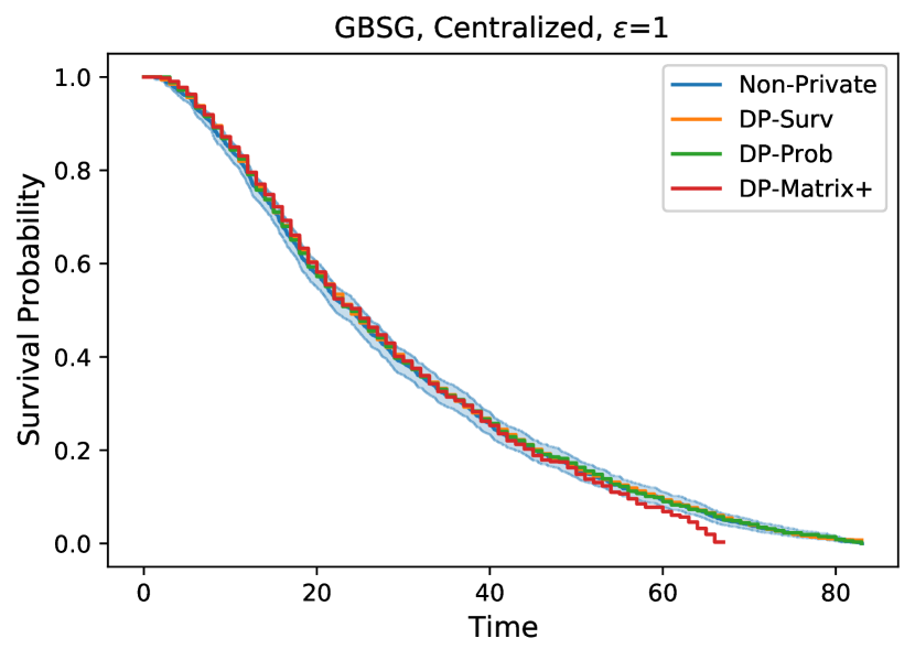
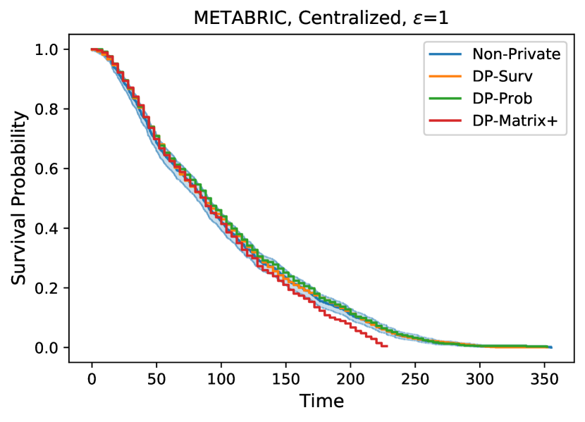
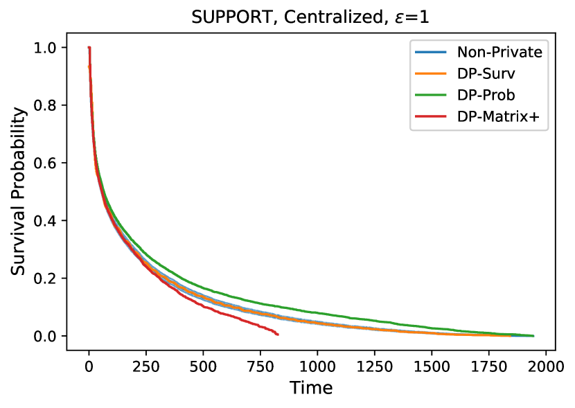
Figure 3. Comparison of all the DP methods in a centralized setting, for $\varepsilon=1$ and one random run of the DP algorithms. The blue shaded region shows the confidence area of the non-private dataset.

Based on the two previous sections, we now know that our surrogate dataset generation algorithm is reliable and we were able to pick suitable hyperparameters for our DP algorithms. Now we would like to study their performance in a centralized setting. The goal is to match the performance of a non-private KM curve as best as we can and with the best privacy guarantee (lower $\varepsilon$ values) possible.

Setup

Since any DP algorithm is based on random noise generation, we run all our DP methods for 5 independent runs to inspect their stability (or instability). We report the highest and lowest obtained value over these 5 runs for $p-$value, median and survival percentage at $t=\{0.25T_{\max},0.5T_{\max},0.75T_{\max}\}$ which represent the survival percentage at the beginning of a study, in the middle point and near the end of the study.

Table 5 shows the results of applying DP-Matrix⁺ , DP-Surv and DP-Prob on all datasets. We analyse the results for $\varepsilon=1$ as this theoretically falls into the tight privacy guarantee regime (Ponomareva et al., 2023). For the non-DP dataset, we show the confidence intervals of the KM curve based on its variance (Equation 18) in parentheses. For DP methods, in square brackets we report the maximum and minimum value over 5 runs. We also demonstrate these results for one random run of the DP algorithms in Figure 3, where the blue line is the survival curve for the non-private dataset and the shaded blue region is its corresponding confidence area. The figures for $\varepsilon={0.5,5}$ can be found in Appendix C.

DP-Surv Performance

Our DP-Surv method shows consistent performance across multiple runs of the DP algorithm for all datasets with very stable survival percentages and median estimates. Its $p-$value is always significantly above the commonly-acceptable statistical difference of $0.05$, and the median as well as survival percentages fall within the confidence interval for all the 3 non-private datasets.

DP-Prob Performance

Our second suggested method, DP-Prob, also performs very well in this tight privacy regime, coming second after DP-Surv, in terms of highest consistent $p-$value across all datasets, with the $p-$value falling below $0.05$ only for SUPPORT dataset. For different runs of the algorithm, we also observe very consistent and stable survival percentages which are always within the confidence interval of all the non-private datasets for GBSG and METABRIC. For SUPPORT we observe a worse performance. As mentioned, SUPPORT is the dataset with the fastest fall of the survival rate in the beginning of the time-frame of the study (this can be seen better in Figure3), and this puts the median in a very sensitive area where a lot of points are experiencing an event and the survival percentages are very close to each other for different times in the study. This issue seems to affect DP-Prob more negatively compared to DP-Surv which shows a good approximation even for median.

DP-Matrix⁺ Performance

DP-Matrix⁺  has the worst performance among the three DP methods, with $p-$value dropping lower than $0.05$ in SUPPORT in all 5 random runs and in METABRIC for at least one of the random runs. We especially see a degradation in the performance of DP-Matrix⁺  towards the endpoint of the study at $0.75\%T_{\max}$ in METABRIC and SUPPORT. The reason is probably the post-processing step as described in Equation 7 of Section 4.2 (corresponding to line 5 of Algorithm 1 in the original paper (Gondara and Wang, 2020)), where the noisy at-risk group is calculated based on the previous step. If we restrict the noisy death numbers to be positive, the noise causes the risk set to drop faster than the original dataset and deplete quickly towards the end of the study. We also see the same issue as DP-Prob for the estimation of median in SUPPORT.

As mentioned in the discussion of Section 3, DP-Matrix only protects the count numbers whereas DP-Surv and DP-Prob offer protection also over time of events, due to our chosen equidistant discretization method. This means that the original DP-Matrix method is not directly comparable with our methods. Moreover, based on our centralized experiments, we observed that even our upgraded version, DP-Matrix⁺ , suffers towards the maximum duration of the datasets. For these reasons, we decide to only focus on DP-Surv and DP-Prob in our de-centralized experiments in the next sections.

Table 5. Performance of the DP methods in the centralized setting for event $e=1$. The goal is to match the survival percentages of the non-private dataset.

		$p$- value	median survival time	$25\%$ $T_{\text{max}}$	$50\%$ $T_{\text{max}}$	$75\%$ $T_{\text{max}}$
GBSG	centralized, non-private	-	$24(22;25)$	$0.58(0.55;0.60)$	$0.24(0.22;0.26)$	$0.08(0.07;0.11)$
	DP-Surv ($\varepsilon=1$)	$[0.30,0.36]$	$[24,24]$	$[0.58,0.58]$	$[0.24,0.25]$	$[0.08,0.08]$
	DP-Prob ($\varepsilon=1$)	$[0.24,0.65]$	$[24,25]$	$[0.57,0.58]$	$[0.24,0.24]$	$[0.08,0.09]$
	DP-Matrix+  ($\varepsilon=1$)	$[0.00,0.30]$	$[22,25]$	$[0.54,0.58]$	$[0.17,0.24]$	$[0.00,0.06]$
METABRIC	centralized, non-private	-	$86(81;90)$	$0.49(0.46;0.51)$	$0.16(0.14;0.18)$	$0.02(0.01;0.03)$
	DP-Surv ($\varepsilon=1$)	$[0.43,0.63]$	$[84,88]$	$[0.48,0.48]$	$[0.16,0.17]$	$[0.02,0.02]$
	DP-Prob ($\varepsilon=1$)	$[0.07,0.33]$	$[88,92]$	$[0.48,0.50]$	$[0.16,0.17]$	$[0.02,0.03]$
	DP-Matrix+  ($\varepsilon=1$)	$[0.01,0.67]$	$[84,88]$	$[0.47,0.48]$	$[0.12,0.16]$	$[0.00,0.02]$
SUPPORT	centralized, non-private	-	$57(53;61)$	$0.14(0.13;0.15)$	$0.05(0.04;0.05)$	$0.01(0.01;0.01)$
	DP-Surv ($\varepsilon=1$)	$[0.71,0.94]$	$[58,58]$	$[0.14,0.14]$	$[0.05,0.05]$	$[0.01,0.01]$
	DP-Prob ($\varepsilon=1$)	$[0.00,0.00]$	$[60,64]$	$[0.16,0.17]$	$[0.07,0.08]$	$[0.02,0.03]$
	DP-Matrix+  ($\varepsilon=1$)	$[0.00,0.00]$	$[56,58]$	$[0.11,0.13]$	$[0.00,0.01]$	$[0.00,0.01]$

5.6. Collaboration

In this section, we study the performance of our DP methods when they are deployed to assist with the construction of a private KM curve over the data that is spread among multiple collaborating site. The goal is to match the KM curve obtained over the collection of the data (equivalent to the centralized setting), with an acceptable privacy guarantee.

According to our overall workflow as shown in Figure 2 of Section 4, to utilize either DP-Surv or DP-Prob, we can take one of the 6 possible routs for this privacy-preserving collaboration:

1. DP-Surv pooled (Path A): DP-Surv is applied locally by each client, then private surrogate datasets are generated and shared with the central server. The pooled collection of all private datasets is used to construct the final KM curve.

2. DP-Surv Averaged $\hat{S}^{\prime}$ (Path B): DP-Surv is applied locally by each client, local private KM curves $\hat{S}^{\prime}$ are shared, an average is taken over them and then a global private surrogate dataset is generated to calculate the metrics.

3. DP-Surv Averaged $\hat{y}^{\prime}$ (Path C): DP-Surv is applied locally by each client, local private probability function is calculated and shared, an average is taken over these local $\hat{y}^{\prime}$s and a global private surrogate dataset is generated using the average. The final private and global KM estimator is calculated using this surrogate dataset.

4. DP-Prob pooled (Path D): DP-Prob is applied locally by each client, private local surrogate datasets are generated and shared with the central server. The pooled collection of all private datasets is used to construct the final KM curve and metrics.

5. DP-Prob Averaged $\hat{S}^{\prime}$ (Path E): DP-Prob is applied locally by each client, local private KM curves $\hat{S}^{\prime}$ are calculated as a function of local $\hat{y}^{\prime}$ by clients and shared, an average is taken over them and then a global private surrogate dataset is generated to calculate the metrics and construct the final global and private KM curve.

6. DP-Prob Averaged $\hat{y}^{\prime}$ (Path F): DP-Prob is applied locally by each client, local private probability function is calculated and shared, an average is taken over these local $\hat{y}^{\prime}$s and a global private surrogate dataset is generated using the average. This dataset is then used to calculate the metrics for the global, private KM estimator.

Setup

We consider the case where 10 sites are collaborating with each other in order to jointly build a KM estimator over the collection of their datasets. For this purpose, we first shuffle each dataset then split it into 10 parts with equal number of datapoints for each client. Again, to analyse the stability of our DP methods, we run all our DP methods for 5 independent runs and we report the highest and lowest obtained value over these 5 runs for $p-$value, median and survival percentage at $t=\{0.25T_{\max},0.5T_{\max},0.75T_{\max}\}$.

Sensitivity calculation and privacy

An important problem when dealing with multiple sites using differential privacy, is calculating the correct sensitivity and privacy budget. We set all the hyperparameters, such as maximum time of the dataset, discretization bin size $b$ and the fraction of the coefficients of DCT $k$ with the same values across all collaborating sites. We use the minimum of the number of local datapoints across all sites as the chosen $n_{\textit{tot}}$ for the local deployment of DP-Surv and DP-Prob. This number will be used to calculate the sensitivity of the noise added locally by each client. This gives a upper bound on the privacy budget spending of the whole system and results in the theoretically worst expected possible utility, because all clients are using a sensitivity that is larger or equal to their true local sensitivity. But this is necessary to ensure that our algorithm remains differentially private. This issue will especially become important in the upcoming Section 5.7 where we look at the uneven distribution of data among clients.

Table 6, shows the results for privacy budget $\varepsilon=1$ and the 6 possible paths. For DP methods we report the lowest and highest value of 5 random runs in square brackets. For the non-private centralized dataset we report the confidence intervals in parantheses.

Performance of DP-Surv Based Methods

at first glance, we can observe that for all dataset the DP-Surv-based methods always achieve a relatively high $p-$value compared to the common significance level of 0.05. All the estimated private median times fall within the confidence interval of the non-DP centralized estimate. Also all the survival percentages show no more than $2\%$ difference from the non-DP centralized value.

An interesting observation when comparing paths A, B and C, is their comparable performances. For the survival percentages, we do not see a difference of more than $2\%$ between these 3 paths in each dataset. The median difference is also at most 4 units of time in all datasets. This shows that averaging the private survival functions or the private probability functions is a reasonable solution for collaboration schemes and very close to sharing the private datasets. This is a strong finding and ultimately gives the participants the flexibility to choose which path they want to take to jointly build a model.

Similar to the centralized application of DP-Surv, we observe very stable results between multiple runs, with $2\%$ maximum difference among survival percentages and 4 units of time difference for median time, among all datasets, compared to the non-private centralized baseline. All in all, although we are in a very tight privacy regime of $\varepsilon=1$, we see a very strong and stable performance for all 3 paths which are based on our DP-Surv method.

Performance of DP-Prob Based Methods

For this stringent privacy-guarantee regime, the DP-Prob-based paths do not work as well as the DP-Surv method according to $p-$value. This shows that the DP-Prob method is more sensitive to the amount of DP-noise added for a specific $\varepsilon$ level, compared to DP-Surv.

Compared to DP-Surv-based methods, we see more deviation between different runs of the DP algorithm for paths D, E and F and this is again due to the more sensitive response of DP-Prob to noise.

Table 6. Collaboration with even data split for $e=1$

			$p$- value	median survival time	$25\%$ $T_{\text{max}}$	$50\%$ $T_{\text{max}}$	$75\%$ $T_{\text{max}}$
GBSG	centralized, non-private		-	$24(22;25)$	$0.58(0.55;0.60)$	$0.24(0.22;0.26)$	$0.08(0.07;0.10)$
		pooled	$[0.19,0.73]$	$[24,25]$	$[0.58,0.59]$	$[0.24,0.25]$	$[0.07,0.09]$
	DP-Surv ($\varepsilon=1$)	Averaged $\hat{S}^{\prime}$	$[0.24,0.40]$	$[24,24]$	$[0.58,0.58]$	$[0.24,0.25]$	$[0.08,0.09]$
		Averaged $\hat{y}^{\prime}$	$[0.24,0.38]$	$[24,24]$	$[0.58,0.58]$	$[0.25,0.25]$	$[0.08,0.09]$
		pooled	$[0.00,0.00]$	$[25,28]$	$[0.59,0.63]$	$[0.28,0.32]$	$[0.11,0.14]$
	DP-Prob ($\varepsilon=1$)	Averaged $\hat{S}^{\prime}$	$[0.00,0.00]$	$[26,28]$	$[0.60,0.63]$	$[0.29,0.31]$	$[0.11,0.13]$
		Averaged $\hat{y}^{\prime}$	$[0.00,0.00]$	$[26,28]$	$[0.61,0.62]$	$[0.29,0.32]$	$[0.11,0.14]$
METABRIC	centralized, non-private		-	$86(81;90)$	$0.49(0.46;0.51)$	$0.16(0.14;0.18)$	$0.02(0.01;0.03)$
		pooled	$[0.25,0.96]$	$[84,84]$	$[0.47,0.49]$	$[0.15,0.17]$	$[0.00,0.01]$
	DP-Surv ($\varepsilon=1$)	Averaged $\hat{S}^{\prime}$	$[0.31,0.69]$	$[84,88]$	$[0.48,0.48]$	$[0.16,0.17]$	$[0.02,0.02]$
		Averaged $\hat{y}^{\prime}$	$[0.35,0.59]$	$[84,88]$	$[0.48,0.49]$	$[0.16,0.17]$	$[0.02,0.02]$
		pooled	$[0.00,0.00]$	$[100,108]$	$[0.55,0.58]$	$[0.25,0.26]$	$[0.08,0.09]$
	DP-Prob ($\varepsilon=1$)	Averaged $\hat{S}^{\prime}$	$[0.00,0.00]$	$[96,104]$	$[0.53,0.57]$	$[0.25,0.27]$	$[0.09,0.10]$
		Averaged $\hat{y}^{\prime}$	$[0.00,0.00]$	$[100,104]$	$[0.55,0.65]$	$[0.24,0.27]$	$[0.09,0.11]$
SUPPORT	centralized, non-private		-	$57(53;61)$	$0.14(0.13;0.15)$	$0.05(0.04;0.05)$	$0.01(0.01;0.01)$
		pooled	$[0.01,0.06]$	$[56,58]$	$[0.12,0.13]$	$[0.04,0.04]$	$[0.00,0.01]$
	DP-Surv ($\varepsilon=1$)	Averaged $\hat{S}^{\prime}$	$[0.26,0.46]$	$[58,58]$	$[0.13,0.14]$	$[0.04,0.05]$	$[0.00,0.01]$
		Averaged $\hat{y}^{\prime}$	$[0.16,0.47]$	$[58,60]$	$[0.13,0.14]$	$[0.04,0.05]$	$[0.00,0.01]$
		pooled	$[0.00,0.00]$	$[270,280]$	$[0.40,0.41]$	$[0.25,0.26]$	$[0.11,0.13]$
	DP-Prob ($\varepsilon=1$)	Averaged $\hat{S}^{\prime}$	$[0.00,0.00]$	$[296,306]$	$[0.42,0.42]$	$[0.26,0.27]$	$[0.12,0.13]$
		Averaged $\hat{y}^{\prime}$	$[0.00,0.00]$	$[294,304]$	$[0.41,0.42]$	$[0.26,0.26]$	$[0.12,0.13]$

5.7. Collaboration: A Broader View

So far we only studied the case of even split of data, where each client has the same number of data point as the others. We now would like to explore more realistic and challenging scenarios, which include uneven distribution of data (similar to previous works on distributed medical data (e.g. Duan et al., 2018)). For this reason we look at two cases: a) One client possesses $50\%$ of all data and b) one client has only $5\%$ of the data.

Our results in the previous section show that DP-Surv-based paths (A, B and C) work best for collaboration with even split of data. Since sharing the private local survival functions $\hat{S}^{\prime}$ would be the most natural and practical scenario among participants, and also since sharing a discrete function is more lightweight compared to sharing datasets when collaborating, we choose path B for our experiments in this section.

Figure 4 shows the results for $\varepsilon=1$ and 10 clients and one random run of path B. For uneven splits, the minority site (the site which has different amount of data compared to other 9 sites) receives either $5\%$ or $50\%$ of all the randomly-shuffled data and the rest of the dataset is split evenly among the 9 remaining participants. The non-DP centralized case is shown with the blue line with its corresponding blue-shaded confidence interval. We also show the KM curves obtained by each client if they used only their local (non-DP) data. We report the $p-$value to the non-DP centralized case as well as median survival time as p and m, respectively. We also include the complete metrics for DP-Surv-based paths as well as the figures for $\varepsilon=0.5$ in Appendix D.

For all datasets the $p-$value of our DP-Surv method is above the significance level of $0.05$ for all 3 types of data split and the median is always in the confidence interval of the non-private centralized setting. We observe that our private curve is always stable and matches the centralized estimator very well, whereas the KM estimator of individual local sites can deviate from the centralized case and are non-smooth, in general.

We see that the collaboration, even when DP-noise is added to guarantee the privacy, is still beneficial for individual sites: For GBSG, our DP method estimates the median of the non-private centralized estimator better than 7, 9 and 4 local sites for even, uneven with $5\%$ and uneven with $50\%$ data splits, respectively. For METABRIC, our DP-Surv method outperforms the local sites in 7, 7 and 6 instances for even, uneven with $5\%$ and uneven with $50\%$ split in terms of median estimation. These numbers are 6, 6 and 8 for SUPPORT dataset, respectively. Most noticably, we see that the minority site which receives $5\%$ of the data (middle column) gains from this collaboration and its local dataset is not informative enough to generalized to the behavior of the whole population.

This is an important finding and shows that there is always an incentive for individual data holders to collaborate for a better estimation of the KM curves. Given that we are applying tight privacy guarantees, the privacy of the datasets of these individual collaborator will not be compromised.

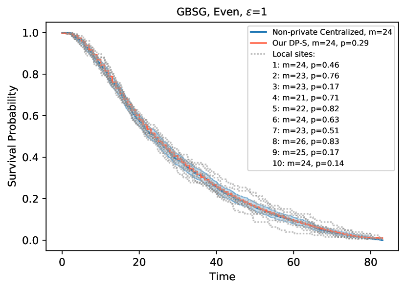
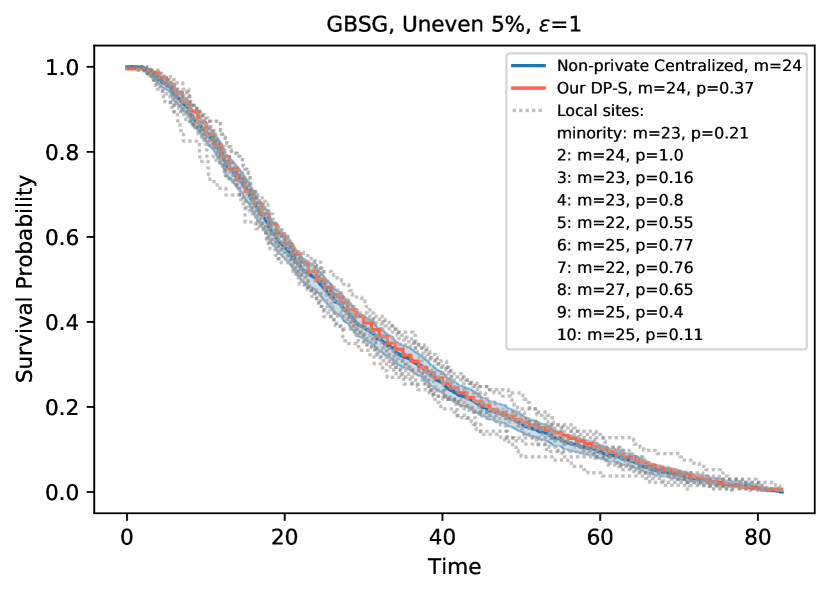
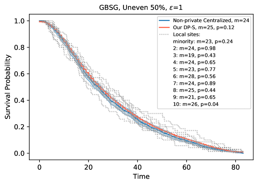
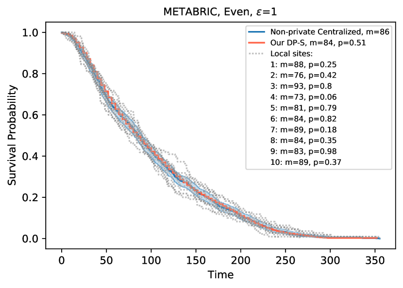
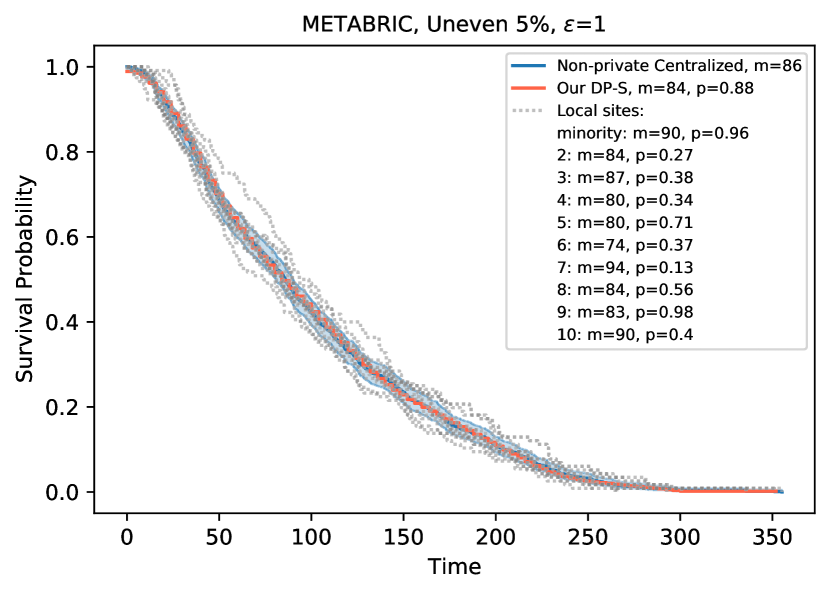
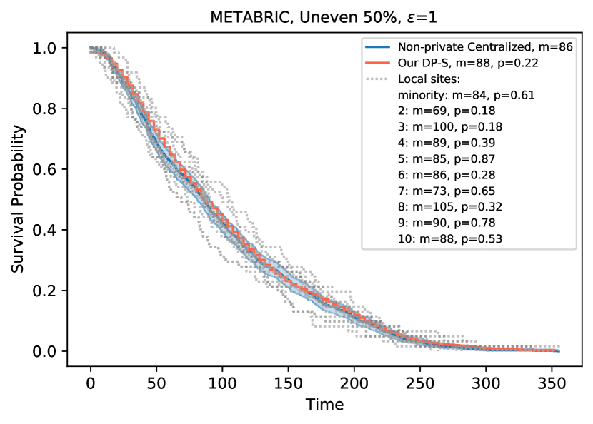
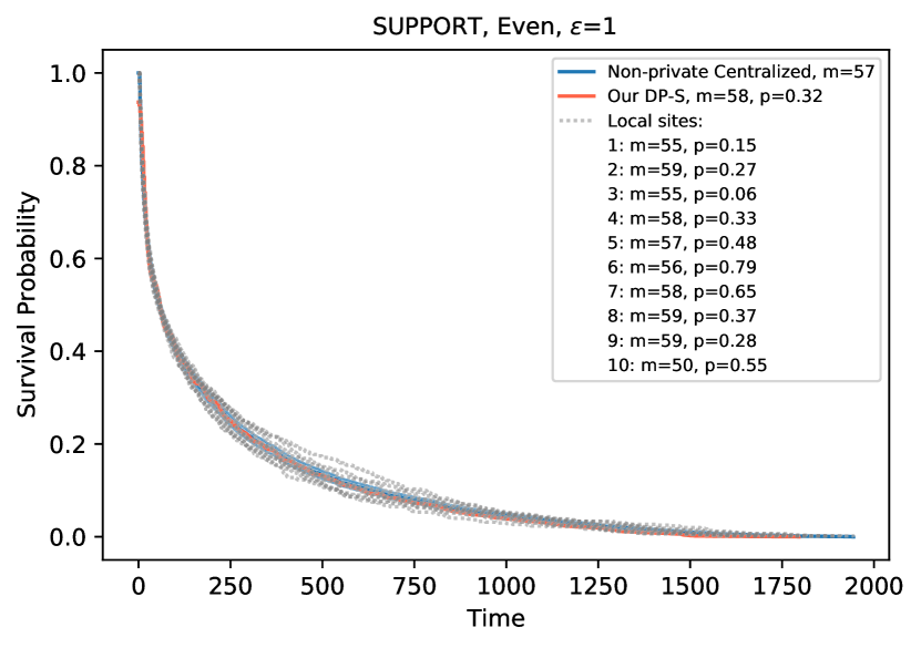
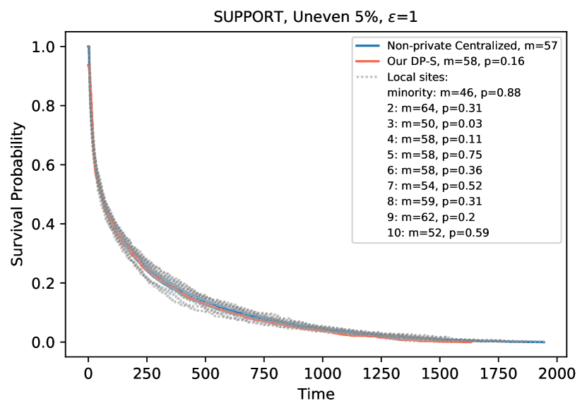
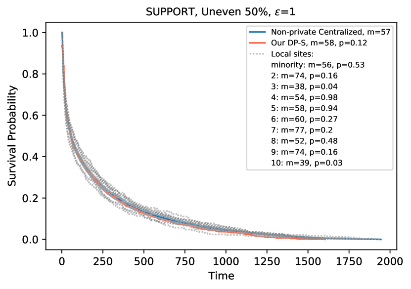
Figure 4. Collaboration among 10 sites for 3 types of data splitting. Our private DP-Surv method is shown with the red line. The median and the $p-$value to the non-private, centralized estimator is shown by m and p for our method and also for each site when only the local data is used to construct the KM curve.

5.8. Summary of Our Findings

Through our experiments we found out that:

1. Our surrogate dataset generation method is a reliable way to generate a surrogate dataset that match the performance of the real dataset, with access to only the probability mass function of the data.

2. Our DP-Surv and DP-Prob method show a near perfect performance in a centralized setting and for very low privacy budgets.

3. Our DP-Surv-based paths for collaboration are all comparable, very stable and return very accurate estimates with respect to the non-DP centralized setting, where we assume all data is stored on a central server.

4. DP-Surv-based paths can successfully be used for uneven splits of data and they offer a strong incentive for collaboration among multiple data centers.

6. Related Work

The power of Kaplan-Meier estimators, especially for medical applications, lies in the fact that they make no assumptions on the underlying factors that contribute to differences in the survival behavior of different populations and can directly be constructed from the data and readily used to draw conclusions. Therefore, these are widely used in the medical domain for treatment assessment (e.g. Castro, 1995; Rossi et al., 2012), gene expression affect on survival (e.g. Mihály et al., 2013; Glinsky et al., 2004), etc.

In presence of a large dataset, the quality of the Kaplan-Meier estimators improves and they generalizes better to the true properties of a population. However, a large enough dataset is not necessarily always available. Survival dataset are usually distributed among multiple centers that are in charge of collecting them, for example, hospitals or banks. This gives rise to the need for collaboration among multiple centers that work on the same goal (e.g. cancer treatment), to form a more accurate and more generalizable model.

KM curves are constructed as a function of the data. In many applications, and especially the medical survival analysis, these data contain sensitive information about the individuals and protection of privacy of these individuals is a matter of utmost concern. Naturally, there are many privacy regulations (e.g. Politou et al., 2018; Voigt and Von dem Bussche, 2017; Beverage, 1976; Hodge Jr et al., 1999) that prohibit the sharing of raw data with other centers. Attempts to overcome this issue and to construct a KM estimator in collaboration with multiple centers have mostly focused on secure multi party computation (SMPC)(Froelicher et al., 2021; Vogelsang et al., 2020; von Maltitz et al., 2021) of KM curves based on secure calculation of statistics needed to construct the estimator. However, there are many issues with this approach. Firstly, SMPC schemes do not scale well to larger settings: the cost of computation and communication usually grows very fast. Second, even after using a secure scheme, there is still privacy risks for the dataset when the summary statistics are shared publicly. An outside adversary can still perform attacks such as re-identification (El Emam et al., 2011; Rocher et al., 2019) or inference (Backes et al., 2016; Homer et al., 2008) on summary statistics.

A practical and strong method to guarantee the privacy of the dataset is using differential privacy (Dwork and Roth, 2014). In contrast to SMPC, differential privacy by definition has the power to neutralize adversarial attacks. DP can be applied either directly on the dataset or functions of the dataset. One way to incorporate DP in the Kaplan-Meier estimation is to add Laplace noise to the number counts in the survival dataset (Gondara and Wang, 2020). This method is restrictive, because always an access to the number counts at specific times of events is required. It also does not offer privacy for the times of events and these will still be published with no DP randomness applied to them.

In our paper, we take advantage of the probability density estimator (Kvamme et al., 2019; Lee et al., 2018), which is an alternative statistic, closely related to the Kaplan-Meier function, to construct surrogate datasets solely based on KM function or probability function. This allows us to offer DP methods that are directly applicable on these two functions and readily converting between summary statistics and (surrogate) dataset. Our first DP method which is inspired by (Kerkouche et al., 2021; Rastogi and Nath, 2010), tweaks the KM function in its discrete cosine space. Our second DP method tweaks the probability function. By sampling these two functions in their time dimension, we are able to offer privacy on the times of events. Our methods show improvement in the privacy budget ($\varepsilon$) spending for the same utility compared to the previously-suggested method (Goel et al., 2010) and this allows us to expand our methods to a collaborative setting. We are able to construct accurate, private and collaborative KM curves which satisfy tight privacy guarantees ($\varepsilon=1$) for various data splitting types among clients.

7. Conclusion and Future Work

In this work, we take a broad view on different representations of survival statistics and show how rapidly we can convert between these representations. Most notably, we show that we can construct a surrogate dataset solely based on the Kaplan-Meier function. This helps us to apply differential privacy in an effective and straightforward way to survival information with no need to have access to the dataset. In comparison to the previous work, we are able to offer privacy not only on the count numbers but also on times of events, by sampling the survival estimator and probability estimators at equidistant time intervals.

With this broader point of view on different representations, we are able to suggest multiple different routes that a system of collaborating sites can utilize to achieve a global private KM estimation. Utilizing this systematic analysis of different constructions, we find effective methods that deliver a private, collaborative Kaplan-Meier estimator that provides results on par with the non-private, centralized version. We show that our methods are robust against different distributions of data among dataholders and how this can motivate small as well as big medical centers to join our private, collaborative scheme.

We believe that with this concept in mind, exploring other potential DP methods on different representations of survival data is an interesting research direction and can offer paths that not only improve the utility of the final aggregated model but are also applicable on different statistics depending on the requirements of the users.

Appendix A Sensitivity of $\hat{S}(t)$

To apply differential privacy on the Kaplan-Meier estimator $\hat{S}(T)$, we consider the notion of neighboring dataset where one dataset is obtained by changing one data point in the other dataset. So both of our neighboring datasets have the same number of total data points $N$. Here, we measure the value of the KM estimator at equidistant time intervals $t_{i}\in\{t_{0}=0,t_{1}=b,...,T_{\max}\}$ with a fixed distance of $b$ to simultaneously gaurantee the privacy of times of events, as described in Section 3. In this case the most affect one data point might have on $\hat{S}(t)$ is obtained by changing the time of event for a point that experiences the event $e=1$ at time $T_{\max}$ to $t_{1}$. We assume this is true since as described in Section 2.1 the effect of censored data on the calculated value of the Kaplan-Meier curve is minimal (only appearing in the risk set of Equation 2) compared to points that experience the event of interest. And also since the effect of an event happening at time $t$ demonstrates itself in all the calculated KM values of the following timesteps $\geq t$ (see Equation 2). Note that the neighboring datasets will have the same number of data points $N$ and also the same number of events $\sum_{i=1}^{T_{\max}}d_{i}$ and same number of censored points $\sum_{i=1}^{T_{\max}}c_{i}$.

To develop an initial intuition, we start with the case when no censoring data is present in the dataset, as this will be the easiest to bound for sensitivity. Assuming that $\hat{S}(t)$ is measured on a dataset with a total of $N$ datapoints with no censored data, and $S^{\prime}(t)$ is measured for the neighboring dataset obtained by moving the time of the event of a point to $t_{1}$, we have:

$$\hat{S}_{1} = \frac{N-d_{1}}{N},\qquad\hat{S}^{\prime}_{1}=\frac{N-d_{1}-1}{N}$$

(21) $$\Rightarrow \hat{S}_{1}-\hat{S}^{\prime}_{1}=\frac{1}{N}$$

$$\hat{S}_{2} = \hat{S}_{1}.\frac{r_{2}-d_{2}}{r_{2}}=\frac{N-d_{1}}{N}.\frac{N-d_{1}-d_{2}}{N-d_{1}}$$

(22) $$= \frac{N-d_{1}-d_{2}}{N}$$

$$\hat{S}^{\prime}_{2} = \hat{S}^{\prime}_{1}.\frac{r^{\prime}_{2}-d_{2}}{r^{\prime}_{2}}=\frac{N-d_{1}-1}{N}.\frac{N-d_{1}-1-d_{2}}{N-d_{1}-1}$$

(23) $$= \frac{N-d_{1}-1-d_{2}}{N}$$

(24) $$\Rightarrow \hat{S}_{2}-\hat{S}^{\prime}_{2}=\frac{1}{N}$$

Where $\hat{S}_{i},d_{i}$ and $r_{i}$ denote the KM estimator, number of events and risk set measured at time $t_{i}$, respectively. The third line is derived from the definition of $\displaystyle{\hat{S}(t)=\hat{S}(t-1)\times\frac{r_{t}-d_{t}}{r_{t}}}$. Now we hypothesize that for the $k$-th term of the survival function we have:

(25) $$\hat{S}_{k} = \frac{N-d_{1}-d_{2}-...-d_{k}}{N}$$

(26) $$\hat{S}^{\prime}_{k} = \frac{N-d_{1}-1-d_{2}-...-d_{k}}{N}$$

and show that for the $k+1$-th term we have:

$$\hat{S}_{k+1} = \hat{S}_{k}\times\frac{r_{k+1}-d_{k+1}}{r_{k+1}}$$

$$= \frac{N-d_{1}-...-d_{k}}{N}.\frac{N-d_{1}-...-d_{k+1}}{N-d_{1}-...-d_{k}}$$

(27) $$= \frac{N-d_{1}-...-d_{k+1}}{N}$$

$$\hat{S}^{\prime}_{k+1} = \hat{S}^{\prime}_{k}\times\frac{r^{\prime}_{k+1}-d_{k+1}}{r^{\prime}_{k+1}}$$

$$= \frac{N-d_{1}-1-...-d_{k}}{N}.\frac{N-d_{1}-1-...-d_{k+1}}{N-d_{1}-1-...-d_{k}}$$

(28) $$= \frac{N-d_{1}-1-...-d_{k+1}}{N}$$

Therefore, we prove by induction that our hypothesis is correct. Now we can calculate the difference of any term $k$ between $S$ and $S^{\prime}$:

$$\hat{S}_{k}-\hat{S}^{\prime}_{k} = \frac{N-d_{1}-...-d_{k}}{N}-\frac{N-d_{1}-1-...-d_{k}}{N}$$

(29) $$= \frac{1}{N}$$

For the last term, there is also a difference between $\hat{S}_{T_{\max}}$ and $\hat{S}^{\prime}_{T_{\max}}$, since now for $\hat{S}^{\prime}$ a datapoint experiencing the event is missing:

$$\hat{S}_{T_{\max}}-\hat{S}^{\prime}_{T_{\max}}=\frac{N-d_{1}-...d_{T_{\max}}}{N}-$$

$$\frac{N-d_{1}-1-...-(d_{T_{\max}}-1)}{N}=\frac{0}{N}$$

So over the time-span of the study the total difference of $\hat{S}$ and $\hat{S}^{\prime}$ would be:

(30) $$\Delta_{1}\hat{S}_{\text{no censor}}=\|\hat{S}-\hat{S}^{\prime}\|_{1}=\frac{T-1}{N}$$

(31) $$\Delta_{2}\hat{S}_{\text{no censor}}=\|\hat{S}-\hat{S}^{\prime}\|_{2}=\frac{\sqrt{T-1}}{N}$$

Where $T$ is the number of time-bins, i.e. $T=T_{\max}/b$.

For when we have censoring in the dataset:

$$\hat{S}_{t}= \frac{N-d_{1}}{N}\frac{N-d_{1}-c_{1}-d_{2}}{N-d_{1}-c_{1}}\times...$$

$$\times\frac{N-d_{1}-...d_{t-1}-c_{1}-....c_{t-1}-d_{t}}{N-d_{1}-...d_{t-1}-c_{1}...-c_{t-1}}$$

(32)

$$\hat{S}^{\prime}_{t}= \frac{N-d_{1}-1}{N}\frac{N-1-d_{1}-c_{1}-d_{2}}{N-1-d_{1}-c_{1}}\times...$$

$$\times\frac{N-1-d_{1}-...d_{t-1}-c_{1}-....c_{t-1}-d_{t}}{N-1-d_{1}-...d_{t-1}-c_{1}...-c_{t-1}}$$

(33)

Lemma 1.

$\forall A,B,c\in\mathbf{N}$ if ($B,B-c>0\land A,c\geq 0\land B\geq A$) :

$$\frac{A-c}{B-c}\leq\frac{A}{B}$$

Proof.

$AB-Bc\leq AB-Ac\Leftrightarrow Bc\geq Ac\Leftrightarrow B\geq A$∎

Lemma 2.

$\forall A,B,c\in\mathbf{N}$ if $B,B-c>0\land A,c\geq 0$:

$$\frac{A}{B}\leq\frac{A}{B-c}$$

Proof.

$AB-Ac\leq AB\Leftrightarrow Ac\geq 0$∎

So we can upper and lower bound each individual $\hat{S}_{t}$ and $\hat{S}^{\prime}_{t}$ by either adding $\sum_{i=1}^{t^{\prime}-1}c_{i}$ to both numerator and denominator of each fraction which represents the new term at time $t^{\prime}$ (for the upper bound) or adding $c_{t^{\prime}}$ to only the denominator of each fraction at time $t^{\prime}$ in the Equation 32 and 33 (for lower bound), that is:

$$\frac{N-d_{1}}{N}\frac{N-d_{1}-c_{1}-d_{2}}{N-d_{1}-c_{1}+c_{1}}\times...$$

$$\frac{N-d_{1}-...d_{t-1}-c_{1}-...c_{t-1}-d_{t}}{N-d_{1}-...d_{t-1}-c_{1}-...c_{t-1}+c_{t-1}}\leq\hat{S}_{t}\leq$$

$$\frac{N-d_{1}}{N}\frac{N-d_{1}-c_{1}+c_{1}-d_{2}}{N-d_{1}-c_{1}+c_{1}}\times...$$

$$\frac{N-d_{1}-...d_{t-1}-c_{1}-...c_{t-1}+c_{1}+...+c_{t-1}-d_{t}}{N-d_{1}-...d_{t-1}-c_{1}-...c_{t-1}+c_{1}+...c_{t-1}}$$

and we can also bound $\hat{S}^{\prime}_{t}$ in the same way. So finally, after cancelling out the consecutive numerators and denominators we are left with:

$$\frac{N-d_{1}...-d_{t}-c_{1}...-c_{t-1}}{N}\leq\hat{S}_{t}$$

(34) $$\leq\frac{N-d_{1}...-d_{t}}{N}$$

$$\frac{N-1-d_{1}...-d_{t}-c_{1}...-c_{t-1}}{N}\leq\hat{S}^{\prime}_{t}$$

(35) $$\leq\frac{N-1-d_{1}...-d_{t}}{N}$$

We know that $S_{t}\geq\hat{S}^{\prime}_{t}$ for all times, because $\hat{S}^{\prime}$ has experienced one extra death in the first time step, so the value of $\hat{S}_{t}-\hat{S}^{\prime}_{t}\geq 0$ at all times. For an upper bound we can subtract the lower bound of $\hat{S}^{\prime}_{t}$ from the upper bound of $\hat{S}_{t}$:

$$\hat{S}_{t}-\hat{S}^{\prime}_{t}\leq \frac{N-d_{1}...-d_{t}}{N}-\frac{N-1-d_{1}...-d_{t}-c_{1}...-c_{t-1}}{N}$$

(36) $$\Rightarrow \hat{S}_{t}-\hat{S}^{\prime}_{t}=\begin{cases}\frac{1}{N}&t=1\\ \frac{1+c_{1}...+c_{t-1}}{N}&1<t<T_{\max}\\ \frac{c_{1}+...+c_{t-1}}{N}&t=T_{\max}\end{cases}$$

if we define $C=\sum^{T_{\max}-1}_{i=1}c_{i}$, we can find a general upper bound over the whole time-span of the study:

$$\Delta_{1}\hat{S}_{\text{w censor}}=\|\hat{S}-\hat{S}^{\prime}\|_{1}=\frac{1}{N}+\frac{1+c_{1}}{N}+...\frac{c_{1}+...c_{T_{\max}-1}}{N}$$

(37) $$\leq\frac{T(1+C)}{N}$$

$$\Delta_{2}\hat{S}_{\text{w censor}}=\|\hat{S}-\hat{S}^{\prime}\|_{2}=\sqrt{(\frac{1}{N})^{2}+(\frac{1+c_{1}}{N})^{2}+...(\frac{c_{1}+...c_{T_{\max}-1}}{N})^{2}}$$

(38) $$\leq\sqrt{(\frac{1+C}{N})^{2}+...+(\frac{1+C}{N})^{2}}=\frac{\sqrt{T}(1+C)}{N}$$

Where $T$ is the number of time-bins, i.e. $T=T_{\max}/b$. Note that this is in line with our proof for the case of no censoring according to Equations 30 and 31. So in general we have:

(39) $$\Delta_{1}\hat{S}=\{(C=0)\rightarrow\frac{T-1}{N},(C\neq 0)\rightarrow\frac{T(1+C)}{N}\}$$

(40) $$\Delta_{2}\hat{S}=\{(C=0)\rightarrow\frac{\sqrt{T-1}}{N},(C\neq 0)\rightarrow\frac{\sqrt{T}(1+C)}{N}\}$$

Appendix B Sensitivity of $\hat{y}(t)$

In this section we derive the sensitivity of $\hat{y}$. The neighboring datasets are defined the same way as in our proof for sensitivity of $\hat{S}$ in Section A: $\mathcal{D^{\prime}}$ is derived from $\mathcal{D}$ by changing the time of event of a point that experiences the event at the end of study $T_{\max}$ to $t=1$, the first time bin in the study. We once more assume that the events are read at equidistant time intervals $t_{i}\in\{t_{0}=0,t_{1}=b,...,T_{\max}\}$ with a fix bin size of $b$. We first derive the sensitivity in absence of censored data and then proceed to the more general case with censored data in the dataset.

We denote the probability mass function of the dataset $\mathcal{D}$ as $\hat{y}$ and the probability mass function of its neighboring dataset $\mathcal{D^{\prime}}$ as $\hat{y}^{\prime}$. According to Equation 4 we have $\hat{y}_{t}=\hat{S}_{t-1}-\hat{S}_{t}$ and $\hat{y}^{\prime}_{t}=\hat{S}^{\prime}_{t-1}-\hat{S}^{\prime}_{t}$, where $\hat{y}_{t}(\hat{y}^{\prime}_{t})$ and $\hat{S}_{t}(\hat{S}^{\prime}_{t})$ indicate the value of the probability mass function and KM estimator at times $t$, respectively. So:

$$\hat{y}_{1}= \hat{S}_{0}-\hat{S}_{1}=1-\frac{N-d_{1}}{N}$$

$$\hat{y}^{\prime}_{1}= \hat{S}_{0}^{\prime}-\hat{S}_{1}^{\prime}=1-\frac{N-d_{1}-1}{N}$$

(41) $$\Rightarrow \hat{y}^{\prime}_{1}-\hat{y}_{1}=\frac{1}{N}$$

According to Equations 27 and 28, we have:

$$\hat{y}_{t}= \frac{N-d_{1}-...d_{t-1}}{N}-\frac{N-d_{1}-...d_{t}}{N}=\frac{d_{t}}{N}$$

$$\hat{y}^{\prime}_{t}= \frac{N-d_{1}-1-...d_{t-1}}{N}-\frac{N-1-d_{1}-...d_{t}}{N}=\frac{d_{t}}{N}$$

(42) $$\Rightarrow \hat{y}^{\prime}_{t}-\hat{y}_{t}=0$$

There is also a difference in the last term due to changing the event of one datapoint from $t=T_{\max}$ to $t=1$:

$$\hat{y}_{T_{\max}}= \frac{N-d_{1}-...d_{T_{\max}-1}}{N}-\frac{N-d_{1}-...d_{T_{\max}}}{N}=\frac{d_{T_{\max}}}{N}$$

$$\hat{y}^{\prime}_{T_{\max}}= \frac{N-d_{1}-1-...d_{T_{\max}-1}}{N}-$$

$$\frac{N-d_{1}-1-...-(d_{T_{\max}}-1)}{N}=\frac{d_{T_{\max}}-1}{N}$$

(43) $$\Rightarrow \hat{y}^{\prime}_{t}-\hat{y}_{t}=\frac{-1}{N}$$

This means that the sensitivity of the probability mass function for datasets with no censoring will be:

(44) $$\Delta_{1}\hat{y}_{\text{no censor}}=\|\hat{y}^{\prime}-\hat{y}\|_{1}=\frac{2}{N}$$

(45) $$\Delta_{2}\hat{y}_{\text{no censor}}=\|\hat{y}^{\prime}-\hat{y}\|_{2}=\frac{\sqrt{2}}{N}$$

Now we derive the sensitivity for the general case of datasets also containing censored datapoints.

$$\hat{y}_{t}=\hat{S}_{t-1}-\hat{S}_{t}=\hat{S}_{t-1}-$$

$$\hat{S}_{t-1}\frac{N-d_{1}-...d_{t-1}-c_{1}-...c_{t-1}-d_{t}}{N-d_{1}-...d_{t-1}-c_{1}-...c_{t-1}}=$$

$$\hat{S}_{t-1}[1-\frac{N-d_{1}-...d_{t-1}-c_{1}-...c_{t-1}-d_{t}}{N-d_{1}-...d_{t-1}-c_{1}-...c_{t-1}}]=$$

(46) $$\hat{S}_{t-1}[\frac{d_{t}}{N-d_{1}-...d_{t-1}-c_{1}-...c_{t-1}}]$$

Where for the first line we use the definition of $S_{t}=S_{t-1}\times\frac{r_{t}-d_{t}}{r_{t}}$. In the same way, we can show that:

$$\hat{y}^{\prime}_{t}=\hat{S}^{\prime}_{t-1}-\hat{S}^{\prime}_{t}$$

(47) $$=\begin{cases}\frac{d_{1}+1}{N}&t=1\\ \hat{S}^{\prime}_{t-1}[\frac{d_{t}}{N-1-d_{1}-...d_{t-1}-c_{1}-...c_{t-1}}]&1<t<T_{\max}\\ \hat{S}^{\prime}_{T_{\max}-1}[\frac{d_{t}-1}{N-1-d_{1}-...d_{t-1}-c_{1}-...c_{t-1}}]&t=T_{\max}\end{cases}$$

here the case of $t=1$ and $t=T_{\max}$ are different because we add and subtract one from $d_{t}$ at these times respectively. Now we can use Lemma 1 and 2 and the same trick we used for $\hat{S}$ to lower and upper bound $\hat{y}_{t}$ and $\hat{y}^{\prime}_{t}$ for $1<t<T_{\max}$:

(48) $$\frac{d_{t}}{N}\leq\hat{y}_{t}\leq\frac{d_{t}+\sum_{i=1}^{t-1}c_{i}}{N}$$

(49) $$\frac{d_{t}}{N}\leq\hat{y}^{\prime}_{t}\leq\frac{d_{t}+\sum_{i=1}^{t-1}c_{i}}{N}$$

and again to find an upper bound on the difference of $|\hat{y}^{\prime}_{t}-\hat{y}_{t}|$ we can subtract the lower bound of $\hat{y}_{t}$ from the upper bound of $\hat{y}^{\prime}_{t}$ (or vice versa):

$$|\hat{y}^{\prime}_{t}-\hat{y}_{t}|=$$

(50) $$\begin{cases}\frac{1}{N}&t=1\\ \frac{d_{t}+\sum_{i=1}^{t-1}c_{i}}{N}-\frac{d_{t}}{N}=\frac{\sum_{i=1}^{t-1}c_{i}}{N}&1<t<T_{\max}\\ \frac{d_{T_{\max}}-1+\sum_{i=1}^{T_{\max}-1}c_{i}}{N}-\frac{d_{T_{\max}}}{N}=\frac{-1+\sum_{i=1}^{T_{\max}-1}c_{i}}{N}&t=T_{\max}\end{cases}$$

Note that this is again consistent with our results for the no censoring case. By defining $C=\sum_{i=1}^{T_{\max}-1}c_{i}$, we can construct a general sensitivity over the whole time-frame of the study:

$$\Delta_{1}\hat{y}_{\text{w censor}}=\|\hat{y}^{\prime}-\hat{y}\|_{1}=\frac{1}{N}+\frac{c_{1}}{N}+...\frac{c_{1}+...c_{T_{\max}-1}-1}{N}$$

(51) $$\leq\frac{TC}{N}$$

$$\Delta_{2}\hat{y}_{\text{w censor}}=\|\hat{y}^{\prime}-\hat{y}\|_{2}=\sqrt{(\frac{1}{N})^{2}+(\frac{c_{1}}{N})^{2}+...(\frac{c_{1}+...c_{T_{\max}-1}}{N})^{2}}$$

(52) $$\leq\sqrt{(\frac{C}{N})^{2}+...+(\frac{C}{N})^{2}}=\frac{\sqrt{T}C}{N}$$

Where $T$ is the number of time-bins, i.e. $T=T_{\max}/b$. And finally we can write the most general case of sensitivity for the probability mass function as:

(53) $$\Delta_{1}\hat{y}=\{(C=0)\rightarrow\frac{2}{N},(C\neq 0)\rightarrow\frac{TC}{N}\}$$

(54) $$\Delta_{2}\hat{y}=\{(C=0)\rightarrow\frac{\sqrt{2}}{N},(C\neq 0)\rightarrow\frac{\sqrt{T}C}{N}\}$$

Appendix C Centralized performance of DP Methods

Here we present the results for our centralized experiments, for other values of privacy budget $\varepsilon$. All the parameters and the procedures are as explained in Section 5.5, however, here we choose two new values of privacy budget $\varepsilon=\{0.5,5\}$. The results are shown in Figure 6 and 5. We observe that for a looser privacy guarantee ($\varepsilon=5$), the performance of all the 3 DP method is comparable and close to the non-private baseline. For tighter privacy regime ($\varepsilon=0.5$), DP-Matrix suffers in all 3 datasets. DP-Prob fails for the more delicate SUPPORT dataset with a very fast slope in KM curve. Our DP-Surv method is the most stable and aligns almost perfectly with the non-private data, for all 3 cases.

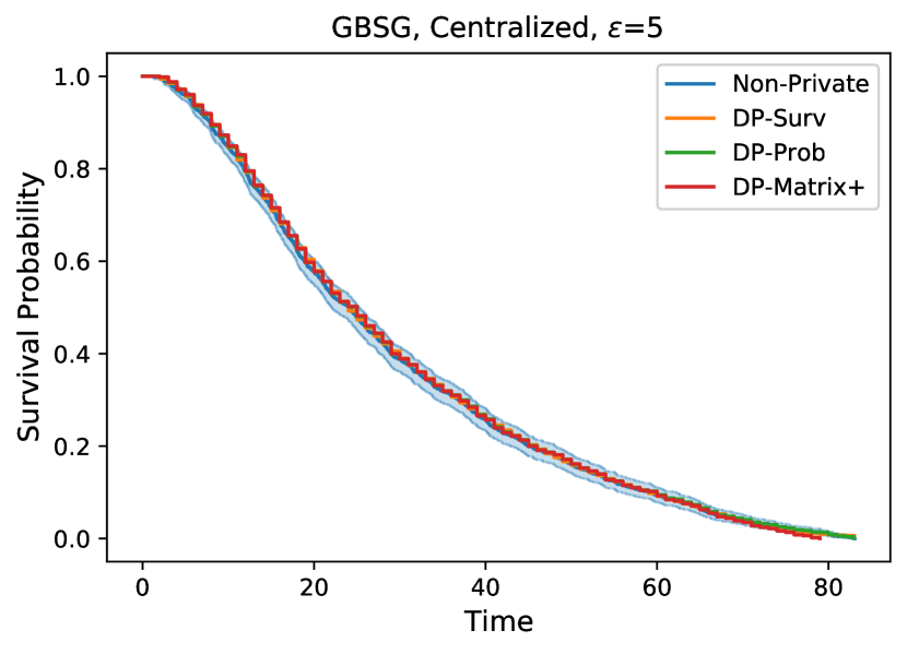
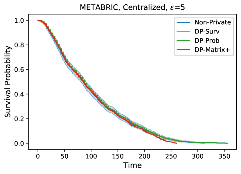
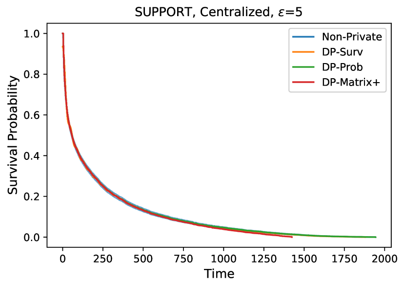
Figure 5. Comparison of all the DP methods in a centralized setting, for $\varepsilon=5$ and one random run of the DP algorithms. The blue shaded region shows the confidence area of the non-private dataset.

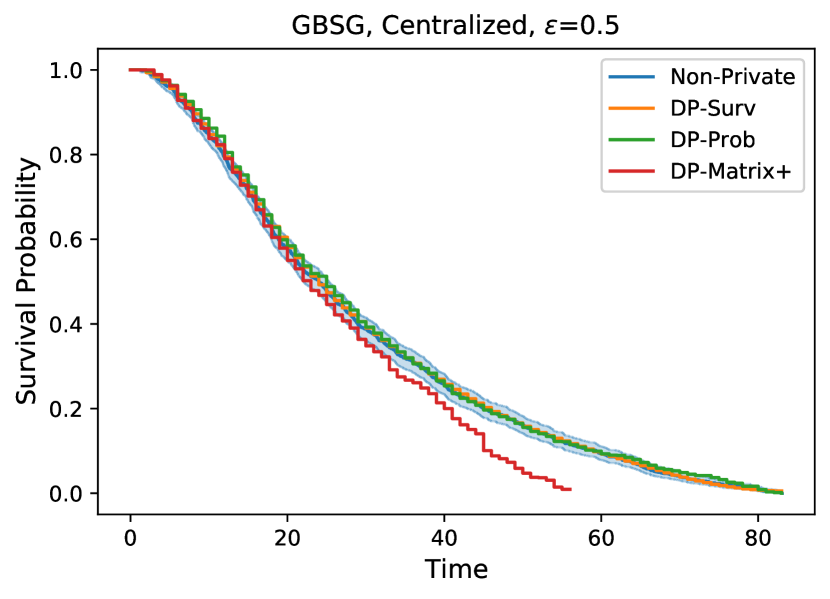
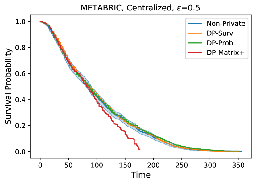
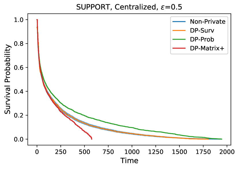
Figure 6. Comparison of all the DP methods in a centralized setting, for $\varepsilon=0.5$ and one random run of the DP algorithms. The blue shaded region shows the confidence area of the non-private dataset.

Appendix D Collaboration

In this section, we first show the complete tables of the metrics for DP-Surv-based methods for uneven splits of the data as explained in Section 5.7. As explained the minority site either receives $5\%$ or $50\%$ of all of the data and the rest is split randomly among the 9 remaining participants. All the parameters and experimental setup is identical to Section 5.7. Table 8 and 7 show the results for paths A, B and C for minority site having $5\%$ and $50\%$ of the data, respectively. As before, the confidence intervals for the non-DP centralized curve is shown with parentheses and for DP curves the lowest and the highest value of the 5 random runs is shown in square brackets.

Split with $50\%$ minority

. As we see in Table 7, the $p-$value never drops below the significance level of 0.05 for GBSG and METABRIC. The median is always within the confidence interval with on exception in path C of METABRIC. This is most likely due to random noise of DP mechanism. And majority of the survival percentages fall within the confidence interval of the non-private case, with the worst case having at most $1\%$ deviation from the confidence interval of the non-private curve. For SUPPORT the $p-$value becomes smaller. This is expected, since SUPPORT has the most drastic fall in the survival percentage in all of our datasets. However, still all the reconstructed private medians fall within the confidence interval of the original non-DP curve. Most of the private survival percentages also agree with the confidence interval of the non-private case, with the worst case having a deviation of at most $1\%$ from the non-DP confidence interval.

Split with $5\%$ minority

In Table 8, we observe that the $p-$value of paths A, B and C are always above the 0.05 significance level for GBSG and METABRIC. In this case, the medians are also always within the confidence interval of the non-DP centralized curve. This is also true for all the survival percentages. For SUPPORT we again observe lower $p-$value, however, the private medians are all within the confidence interval of the non-DP curve. We also observe that the DP survival percentages deviate at most $1\%$ from the correspoding confidence interval of the non-private curve.

Next, we expand our experiments in a collaborative setting for more stringent values of the privacy budget $\varepsilon$. All the parameters and steps are carried out similar to Section 5.7. We show the results for path B and $\varepsilon=0.5$ in Figure 7. In comparison to the experiments explained in Section 5.7, which used a privacy budget of $\varepsilon=1.0$, here we aim for an even tighter privacy regime. We observe that in this very private regime our DP-Surv-based path still performs reasonably well. For GBSG and METABRIC our DP path always has a $p-$value much larger than the significance level of 0.05. The DP estimated medians show at most 2 months deviation from the non-private centralized median for these two datasets. For SUPPORT, we observe that our DP method deviates from the non-private centralized curve for both uneven splits. This is expected, since as explained before, SUPPORT is a special case with a very fast drop in the survival probability of the population. Interestingly, our DP method is still able to estimate the median survival time for SUPPORT with at most 2 days difference from the non-private centralized median of the data.

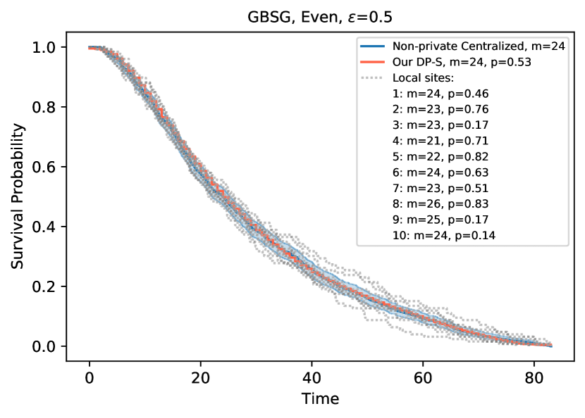
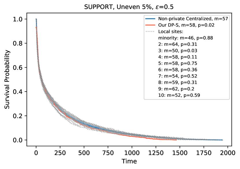
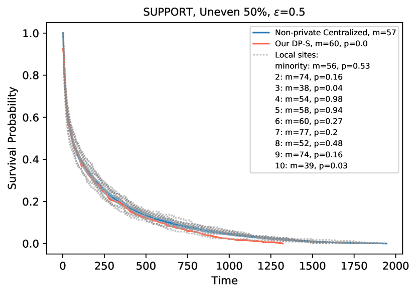
Figure 7. Collaborative private estimation of Kaplan-Meier curves among 10 participating sites for 3 types of data splitting. The blue line shows the non-private centralized case and the red line shows our performance after constructing a joint private estimator. We also plot the locally estimated KM curve with dotted lines for all 10 sites. The median and the $p-$value to the non-DP centralized estimator is shown by m and p.

Table 7. Collaboration with uneven data split with one site receiving $50\%$ of all of the data, for $e=1$ and $\varepsilon=1$

			$p$- value	median survival time	$25\%$ $T_{\text{max}}$	$50\%$ $T_{\text{max}}$	$75\%$ $T_{\text{max}}$
GBSG	centralized, non-private		-	$24(22;25)$	$0.58(0.55;0.60)$	$0.24(0.22;0.26)$	$0.08(0.07;0.10)$
		pooled	$[0.50,0.96]$	$[23,24]$	$[0.56,0.57]$	$[0.22,0.24]$	$[0.06,0.08]$
	DP-Surv ($\varepsilon=1$)	Averaged $\hat{S}^{\prime}$	$[0.07,0.12]$	$[25,25]$	$[0.58,0.59]$	$[0.25,0.26]$	$[0.09,0.10]$
		Averaged $\hat{y}^{\prime}$	$[0.07,0.31]$	$[24,25]$	$[0.59,0.60]$	$[0.25,0.27]$	$[0.09,0.09]$
METABRIC	centralized, non-private		-	$86(81;90)$	$0.49(0.46;0.51)$	$0.16(0.14;0.18)$	$0.02(0.01;0.03)$
		pooled	$[0.41,0.76]$	$[84,84]$	$[0.47,0.48]$	$[0.15,0.16]$	$[0.01,0.02]$
	DP-Surv ($\varepsilon=1$)	Averaged $\hat{S}^{\prime}$	$[0.29,0.57]$	$[84,88]$	$[0.48,0.49]$	$[0.17,0.17]$	$[0.02,0.03]$
		Averaged $\hat{y}^{\prime}$	$[0.06,0.73]$	$[84,92]$	$[0.48,0.50]$	$[0.17,0.18]$	$[0.01,0.04]$
SUPPORT	centralized, non-private		-	$57(53;61)$	$0.14(0.13;0.15)$	$0.05(0.04;0.05)$	$0.01(0.01;0.01)$
		pooled	$[0.02,0.06]$	$[56,58]$	$[0.12,0.13]$	$[0.04,0.04]$	$[0.00,0.01]$
	DP-Surv ($\varepsilon=1$)	Averaged $\hat{S}^{\prime}$	$[0.10,0.21]$	$[58,60]$	$[0.13,0.13]$	$[0.03,0.04]$	$[0.00,0.00]$
		Averaged $\hat{y}^{\prime}$	$[0.10,0.26]$	$[58,60]$	$[0.13,0.14]$	$[0.04,0.04]$	$[0.00,0.00]$

Table 8. Collaboration with uneven data split when one site receives only $5\%$ of all of the data, for $e=1$ and $\varepsilon=1$

			$p$- value	median survival time	$25\%$ $T_{\text{max}}$	$50\%$ $T_{\text{max}}$	$75\%$ $T_{\text{max}}$
GBSG	centralized, non-private		-	$24(22;25)$	$0.58(0.55;0.60)$	$0.24(0.22;0.26)$	$0.08(0.07;0.10)$
		pooled	$[0.44,0.89]$	$[24,24]$	$[0.57,0.59]$	$[0.24,0.24]$	$[0.07,0.08]$
	DP-Surv ($\varepsilon=1$)	Averaged $\hat{S}^{\prime}$	$[0.52,0.79]$	$[24,24]$	$[0.58,0.58]$	$[0.24,0.24]$	$[0.08,0.08]$
		Averaged $\hat{y}^{\prime}$	$[0.43,0.74]$	$[24,24]$	$[0.57,0.58]$	$[0.24,0.25]$	$[0.08,0.08]$
METABRIC	centralized, non-private		-	$86(81;90)$	$0.49(0.46;0.51)$	$0.16(0.14;0.18)$	$0.02(0.01;0.03)$
		pooled	$[0.16,0.66]$	$[84,88]$	$[0.47,0.48]$	$[0.14,0.17]$	$[0.01,0.02]$
	DP-Surv ($\varepsilon=1$)	Averaged $\hat{S}^{\prime}$	$[0.31,0.82]$	$[88,88]$	$[0.49,0.49]$	$[0.16,0.17]$	$[0.02,0.03]$
		Averaged $\hat{y}^{\prime}$	$[0.56,0.97]$	$[84,88]$	$[0.48,0.49]$	$[0.16,0.17]$	$[0.01,0.02]$
SUPPORT	centralized, non-private		-	$57(53;61)$	$0.14(0.13;0.15)$	$0.05(0.04;0.05)$	$0.01(0.01;0.01)$
		pooled	$[0.01,0.03]$	$[56,58]$	$[0.12,0.13]$	$[0.04,0.04]$	$[0.00,0.01]$
	DP-Surv ($\varepsilon=1$)	Averaged $\hat{S}^{\prime}$	$[0.05,0.13]$	$[58,58]$	$[0.13,0.13]$	$[0.03,0.04]$	$[0.00,0.01]$
		Averaged $\hat{y}^{\prime}$	$[0.02,0.15]$	$[58,58]$	$[0.13,0.13]$	$[0.03,0.04]$	$[0.00,0.01]$