Personalized Dictionary Learning for Heterogeneous Datasets

Abstract

We introduce a relevant yet challenging problem named Personalized Dictionary Learning ($\mathsf{PerDL}$), where the goal is to learn sparse linear representations from heterogeneous datasets that share some commonality. In $\mathsf{PerDL}$, we model each dataset’s shared and unique features as global and local dictionaries. Challenges for $\mathsf{PerDL}$ not only are inherited from classical dictionary learning (DL), but also arise due to the unknown nature of the shared and unique features. In this paper, we rigorously formulate this problem and provide conditions under which the global and local dictionaries can be provably disentangled. Under these conditions, we provide a meta-algorithm called Personalized Matching and Averaging ($\mathsf{PerMA}$) that can recover both global and local dictionaries from heterogeneous datasets. $\mathsf{PerMA}$ is highly efficient; it converges to the ground truth at a linear rate under suitable conditions. Moreover, it automatically borrows strength from strong learners to improve the prediction of weak learners. As a general framework for extracting global and local dictionaries, we show the application of $\mathsf{PerDL}$ in different learning tasks, such as training with imbalanced datasets and video surveillance.

1 Introduction

Given a set of $n$ signals $\mathbf{Y}=[\mathbf{y}_{1},\dots,\mathbf{y}_{n}]\in\mathbb{R}^{d\times n}$, dictionary learning (DL) aims to find a dictionary $\mathbf{D}\in\mathbb{R}^{d\times r}$ and a corresponding code $\mathbf{X}=[\mathbf{x}_{1},\dots,\mathbf{x}_{n}]\in\mathbb{R}^{r\times n}$ such that: (1) each data sample $\mathbf{y}_{i}$ can be written as $\mathbf{y}_{i}=\mathbf{D}\mathbf{x}_{i}$ for $1\leq i\leq n$, and (2) the code $\mathbf{X}$ has as few nonzero elements as possible. The columns of the dictionary $\mathbf{D}$, also known as atoms, encode the “common features” whose linear combinations form the data samples. A typical approach to solve DL is via the following optimization problem:

$$\min_{\mathbf{X},\mathbf{D}}\|\mathbf{Y}-\mathbf{D}\mathbf{X}\|_{F}^{2}+\lambda\|\mathbf{X}\|_{\ell_{q}},$$ (DL)

Here $\|\cdot\|_{\ell_{q}}$ is often modeled as a $\ell_{1}$-norm (Arora et al.,, 2015; Agarwal et al.,, 2016) or $\ell_{0}$-(pseudo-)norm (Spielman et al.,, 2012; Liang et al.,, 2022) and has the role of promoting sparsity in the estimated sparse code. Due to its effective feature extraction and representation, DL has found immense applications in data analytics, with applications ranging from clustering and classification (Ramirez et al., (2010); Tošić and Frossard, (2011)), to image denoising (Li et al., (2011)), to document detection(Kasiviswanathan et al., (2012)), to medical imaging (Zhao et al., (2021)), and to many others.

However, the existing formulations of DL hinge on a critical assumption: the homogeneity of the data. It is assumed that the samples share the same set of features (atoms) collected in a single dictionary $D$. This assumption, however, is challenged in practice as the data is typically collected and processed in heterogeneous edge devices (clients). These clients (for instance, smartphones and wearable devices) operate in different conditions (Kontar et al.,, 2017) while sharing some congruity. Accordingly, the collected datasets are naturally endowed with heterogeneous features while potentially sharing common ones. In such a setting, the classical formulation of DL faces a major dilemma: on the one hand, a reasonably-sized dictionary (with a moderate number of atoms $r$) may overlook the unique features specific to different clients. On the other hand, collecting both shared and unique features in a single enlarged dictionary (with a large number of atoms $r$) may lead to computational, privacy, and identifiability issues. In addition, both approaches fail to provide information about “what is shared and unique” which may offer standalone intrinsic value and can potentially be exploited for improved clustering, classification and anomaly detection, amongst others.

With the goal of addressing data heterogeneity in dictionary learning, in this paper, we propose personalized dictionary learning ($\mathsf{PerDL}$); a framework that can untangle and recover global and local (unique) dictionaries from heterogeneous datasets. The global dictionary, which collects atoms that are shared among all clients, represents the common patterns among datasets and serves as a conduit of collaboration in our framework. The local dictionaries, on the other hand, provide the necessary flexibility for our model to accommodate data heterogeneity.

We summarize our contributions below:

• Identifiability of local and global atoms: We provide conditions under which the local and global dictionaries can be provably identified and separated by solving a nonconvex optimization problem. At a high level, our identifiability conditions entail that the true dictionaries are column-wise incoherent, and the local atoms do not have a significant alignment along any nonzero vector.

• Federated meta-algorithm: We present a fully federated meta-algorithm, called $\mathsf{PerMA}$ (Algorithm 1), for solving $\mathsf{PerDL}$. $\mathsf{PerMA}$ only requires communicating the estimated dictionaries among the clients, thereby circumventing the need for sharing any raw data. A key property of $\mathsf{PerMA}$ is its ability to untangle global and local dictionaries by casting it as a series of shortest path problems over a directed acyclic graph (DAG).

• Theoretical guarantees: We prove that, under moderate conditions on the generative model and the clients, $\mathsf{PerMA}$ enjoys a linear convergence to the ground truth up to a statistical error. Additionally, $\mathsf{PerMA}$ borrows strength from strong clients to improve the performance of the weak ones. More concretely, through collaboration, our framework provides weak clients with the extra benefits of averaged initial condition, convergence rate, and final statistical error.

• Practical performance: We showcase the performance of $\mathsf{PerMA}$ on a synthetic dataset, as well as different realistic learning tasks, such as training with imbalanced datasets and video surveillance. These experiments highlight that our method can effectively extract shared global features while preserving unique local ones, ultimately improving performance through collaboration.

1.1 Related Works

Dictionary Learning

Spielman et al., (2012); Liang et al., (2022) provide conditions under which DL can be provably solved, provided that the dictionary is a square matrix (also known as complete DL). For the more complex case of overcomplete DL with $r>d$, Arora et al., (2014, 2015); Agarwal et al., (2016) show that alternating minimization achieves desirable statistical and convergence guarantees. Inspired by recent results on the benign landscape of matrix factorization (Ge et al.,, 2017; Fattahi and Sojoudi,, 2020), Sun et al., (2016) show that a smoothed variant of DL is devoid of spurious local solutions. In contrast, distributed or federated variants of DL are far less explored. Huang et al., (2022); Gkillas et al., (2022) study DL in the federated setting. However, they do not provide any provable guarantees on their proposed method.

Federated Learning & Personalization

Recent years have seen explosive interest in federated learning (FL) following the seminal paper on federated averaging (McMahan et al.,, 2017). Literature along this line has primarily focused on predictive modeling using deep neural networks (DNN), be it through enabling faster convergence (Karimireddy et al.,, 2020), improving aggregation schemes at a central server (Wang et al.,, 2020), promoting fairness across all clients (Yue et al.,, 2022) or protecting against potential adversaries (Bhagoji et al.,, 2019). More recently, the focus has been placed on tackling heterogeneity across client datasets through personalization. The key idea is to allow each client to retain their own tailored model instead of learning one model that fits everyone. Approaches along this line either split weights of a DNN into shared and unique ones and collaborate to learn the shared weights (Liang et al.,, 2020; T Dinh et al.,, 2020), or follow a train-then-personalize approach where a global model is learned and fine-tuned locally, often iteratively (Li et al.,, 2021). Again such models have mainly focused on predictive models. Whilst this literature abounds, personalization that aims to identify what is shared and unique across datasets is very limited. Very recently, personalized PCA (Shi and Kontar,, 2022) was proposed to address this challenge through identifiably extracting shared and unique principal components using distributed Riemannian gradient descent. However, PCA cannot accommodate sparsity in representation and requires orthogonality constraints that may limit its application. In contrast, our work considers a broader setting via sparse dictionary learning.

Notation.

For a matrix $\mathbf{A}$, we use $\|\mathbf{A}\|_{2}$, $\|\mathbf{A}\|_{F}$, $\|\mathbf{A}\|_{1,2}$, and $\|\mathbf{A}\|_{1}$ to denote its spectral norm, Frobenius norm, the maximum of its column-wise 2-norm, and the element-wise 1-norm of $\mathbf{A}$, respectively. We use $\mathbf{A}_{i}$ to indicate that it belongs to client $i$. Moreover, we use $\mathbf{A}_{(i)}$ to denote the $i$-th column of $\mathbf{A}$. We use $\mathcal{P}(n)$ to denote the set of $n\times n$ signed permutation matrices. We define $[n]=\{1,2,\dots,n\}$.

2 $\mathsf{PerDL}$: Personalized Dictionary Learning

In $\mathsf{PerDL}$, we are given $N$ clients, each with $n_{i}$ samples collected in $\mathbf{Y}_{i}\in\mathbb{R}^{d\times n_{i}}$ and generated as a sparse linear combination of $r^{g}$ global atoms and $r_{i}^{l}$ local atoms:

$$\mathbf{Y}_{i}=\mathbf{D}^{*}_{i}\mathbf{X}^{*}_{i},\quad\text{where}\quad\mathbf{D}^{*}_{i}=\begin{bmatrix}\mathbf{D}^{g*}&\mathbf{D}^{l*}_{i}\end{bmatrix},\quad\text{for}\quad 1=1,\dots,N.$$ (1)

Here $\mathbf{D}^{g*}\in\mathbb{R}^{d\times r^{g}}$ denotes a global dictionary that captures the common features shared among all clients, whereas $\mathbf{D}^{l*}_{i}\in\mathbb{R}^{d\times r^{l}_{i}}$ denotes the local dictionary specific to each client. Let $r_{i}=r^{g}+r^{l}_{i}$ denote the total number of atoms in $\mathbf{D}^{*}_{i}$. Without loss of generality, we assume the columns of $\mathbf{D}^{*}_{i}$ have unit $\ell_{2}$-norm. The goal in $\mathsf{PerDL}$ is to recover $\mathbf{D}^{g*}$ and $\{\mathbf{D}^{l*}_{i}\}_{i=1}^{N}$, as well as the sparse codes $\{\mathbf{X}^{*}_{i}\}_{i=1}^{N}$, given the datasets $\{\mathbf{Y}_{i}\}_{i=1}^{N}$. Before presenting our approach for solving $\mathsf{PerDL}$, we first consider the following fundamental question: under what conditions is the recovery of the dictionaries $\mathbf{D}^{g*},\{\mathbf{D}^{l*}_{i}\}_{i=1}^{N}$ and sparse codes $\{\mathbf{X}^{*}_{i}\}_{i=1}^{N}$ well-posed?

To answer this question, we first note that it is only possible to recover the dictionaries and sparse codes up to a signed permutation: given any signed permutation matrix $\mathbf{\Pi}\in\mathcal{P}(r_{i})$, the dictionary-code pairs $(\mathbf{D}_{i},\mathbf{X}_{i})$ and $(\mathbf{D}_{i}\mathbf{\Pi}_{i},\mathbf{\Pi}_{i}^{\top}\mathbf{X}_{i})$ are equivalent. This invariance with respect to signed permutation gives rise to an equivalent class of true solutions with a size that grows exponentially with the dimension. To guarantee the recovery of a solution from this equivalent class, we need the $\mu$-incoherency of the true dictionaries.

Assumption 1 ($\mu$-incoherency).

For each client $1\leq i\leq N$, the dictionary ${\mathbf{D}}^{*}_{i}$ is $\mu$-incoherent for some constant $\mu>0$, that is,

$$\max_{j,k}\left|\left\langle\left({\mathbf{D}}^{*}_{i}\right)_{(j)},\left({\mathbf{D}}^{*}_{i}\right)_{(k)}\right\rangle\right|\leq\frac{\mu}{\sqrt{d}}.$$ (2)

Assumption 1 is standard in dictionary learning (Agarwal et al., (2016); Arora et al., (2015); Chatterji and Bartlett, (2017)) and was independently introduced by Fuchs, (2005); Tropp, (2006) in signal processing and Zhao and Yu, (2006); Meinshausen and Bühlmann, (2006) in statistics. Intuitively, it requires the atoms in each dictionary to be approximately orthogonal. To see the necessity of this assumption, consider a scenario where two atoms of $\mathbf{D}^{*}_{i}$ are perfectly aligned (i.e., $\mu=\sqrt{d}$). In this case, using either of these two atoms achieve a similar effect in reconstructing $\mathbf{Y}_{i}$, contributing to the ill-posedness of the problem.

Our next assumption guarantees the separation of local dictionaries from the global one in $\mathsf{PerDL}$. First, we introduce several signed permutation-invariant distance metrics for dictionaries, which will be useful for later analysis.

Definition 1.

For two dictionaries $\mathbf{D}_{1},\mathbf{D}_{2}\in\mathbb{R}^{d\times r}$, we define their signed permutation-invariant $\ell_{1,2}$-distance and $\ell_{2}$-distance as follows:

$$d_{1,2}(\mathbf{D}_{1},\mathbf{D}_{2}) :=\min_{\mathbf{\Pi}\in\mathcal{P}(r)}\|\mathbf{D}_{1}\mathbf{\Pi}-\mathbf{D}_{2}\|_{1,2},$$ (3)

$$d_{2}(\mathbf{D}_{1},\mathbf{D}_{2}) :=\min_{\mathbf{\Pi}\in\mathcal{P}(r)}\|\mathbf{D}_{1}\mathbf{\Pi}-\mathbf{D}_{2}\|_{2}.$$ (4)

Furthermore, suppose $\mathbf{\Pi}^{*}=\arg\min_{\mathbf{\Pi}\in\mathcal{P}(r)}\|\mathbf{D}_{1}\mathbf{\Pi}-\mathbf{D}_{2}\|_{1,2}$. For any $1\leq j\leq r$, we define

$$d_{2,(j)}(\mathbf{D}_{1},\mathbf{D}_{2}):=\left\|\left(\mathbf{D}_{1}\mathbf{\Pi}^{*}-\mathbf{D}_{2}\right)_{(j)}\right\|_{2}.$$ (5)

Assumption 2 ($\beta$-identifiablity).

The local dictionaries $\left\{{\mathbf{D}}^{l*}_{i}\right\}_{i=1}^{N}$ are $\beta$-identifiable for some constant $0<\beta<1$, that is, there exists no vector ${\mathbf{v}}\in\mathbb{R}^{d}$ with $\|{\mathbf{v}}\|_{2}=1$ such that

$$\max_{1\leq i\leq N}\min_{1\leq j\leq r_{l}}d_{2}\left(\left({\mathbf{D}}^{l*}_{i}\right)_{(j)},{\mathbf{v}}\right)\leq\beta.$$ (6)

Suppose there exists a unit-norm ${\mathbf{v}}$ satisfying (6) for some small $\beta>0$. This implies that ${\mathbf{v}}$ is sufficiently close to at least one atom from each local dictionary. Indeed, one may treat this atom as part of the global dictionary, thereby violating the identifiability of local and global dictionaries. On the other hand, the infeasibility of  (6) for large $\beta>0$ implies that the local dictionaries are sufficiently dispersed, which in turn facilitates their identification.

With the above assumptions in place, we are ready to present our proposed optimization problem for solving $\mathsf{PerDL}$:

$$\min_{\mathbf{D}^{g},\{\mathbf{D}_{i}\},\{\mathbf{X}_{i}\}}\sum_{i=1}^{N}\|\mathbf{Y}_{i}-\mathbf{D}_{i}\mathbf{X}_{i}\|_{F}^{2}+\lambda\sum_{i=1}^{N}\|\mathbf{X}_{i}\|_{\ell_{q}},\quad\mathrm{s.t.}\ \ \left(\mathbf{D}_{i}\right)_{(1:r^{g})}=\mathbf{D}^{g}\quad\mathrm{for}\quad 1\leq i\leq N.$$ (PerDL-NCVX)

For each client $i$, PerDL-NCVX aims to recover a dictionary-code pair $(\mathbf{D}_{i},\mathbf{X}_{i})$ that match $\mathbf{Y}_{i}$ under the constraint that dictionaries for individual clients share the same global components.

3 Meta-algorithm of Solving PerDL

In this section, we introduce our meta-algorithm (Algorithm 1) for solving PerDL-NCVX, which we call Personalized Matching and Averaging ($\mathsf{PerMA}$).

Algorithm 1 $\mathsf{PerMA}$: Federated Matching and Averaging

1:  Input: $\{\mathbf{Y}_{i}\}_{i=1}^{N}$.

2:  for client $i=1,...,N$ do

3:     Client: Obtain $\mathbf{D}^{(0)}_{i}$ based on $\mathbf{Y}_{i}$. // Initialization step

4:     Client: Send $\mathbf{D}^{(0)}_{i}$ to the server.

5:  end for

6:  Server: $\left(\mathbf{D}^{g,(0)},\{\mathbf{D}^{l,(0)}_{i}\}_{i=1}^{N}\right)=\texttt{global\_matching}\left(\{\mathbf{D}^{(0)}_{i}\}_{i=1}^{N}\right)$// Separating local from global dictionaries

7:  Server: Broadcast $\left(\mathbf{D}^{g,(0)},\{\mathbf{D}^{l,(0)}_{i}\}_{i=1}^{N}\right)$

8:  for $t=0,1,\dots,T$ do

9:     for client $i=1,...,N$ do

10:         Client: $\left(\mathbf{D}^{g,(t+1)}_{i},\mathbf{D}^{l,(t+1)}_{i}\right)=\texttt{local\_update}\left(\mathbf{Y}_{i},\mathbf{D}^{g,(t)},\mathbf{D}^{l,(t)}_{i}\right)$// Updating the local and global dictionaries for each client

11:        Client: Send $\mathbf{D}^{g,(t+1)}_{i}$ to the server.

12:     end for

13:     Server: Calculate $\mathbf{D}^{g,(t+1)}=\frac{1}{N}\sum_{i=1}^{N}\mathbf{D}^{g,(t+1)}_{i}$.// Averaging global dictionaries

14:     Server: Broadcast $\mathbf{D}^{g,(t+1)}$.

15:  end for

16:  return  $\left(\mathbf{D}^{g,(T)},\{\mathbf{D}^{l,(T)}_{i}\}_{i=1}^{N}\right)$.

In what follows, we explain the steps of $\mathsf{PerMA}$:

Local initialization (Step 3):

$\mathsf{PerMA}$ starts with a warm-start step where each client runs their own initialization scheme to obtain $\mathbf{D}^{(0)}_{i}$. This step is necessary even for the classical DL to put the initial point inside a basin of attraction of the ground truth. Several spectral methods were proposed to provide a theoretically good initialization(Arora et al.,, 2015; Agarwal et al.,, 2016), while in practice, it is reported that random initialization followed by a few iterations of alternating minimization approach will suffice (Ravishankar et al.,, 2020; Liang et al.,, 2022).

Global matching scheme (Step 6)

Given the clients’ initial dictionaries, our global matching scheme separates the global and local parts of each dictionary by solving a series of shortest path problems on an auxiliary graph. Then, it obtains a refined estimate of the global dictionary via simple averaging. A detailed explanation of this step is provided in the next section.

Dictionary update at each client (Step 10)

During each communication round, the clients refine their own dictionary based on the available data, the aggregated global dictionary, and the previous estimate of their local dictionary. A detailed explanation of this step is provided in the next section.

Global aggregation (Step 13)

At the end of each round, the server updates the clients’ estimate of the global dictionary by computing their average.

A distinguishing property of $\mathsf{PerMA}$ is that it only requires the clients to communicate their dictionaries and not their sparse codes. In fact, after the global matching step on the initial dictionaries, the clients only need to communicate their global dictionaries, keeping their local dictionaries private.

3.1 Global Matching and Local Updates

In this section, we provide detailed implementations of global_matching and local_update subroutines in $\mathsf{PerMA}$ (Algorithm 1).

Given the initial approximations of the clients’ dictionaries $\{\mathbf{D}_{i}^{(0)}\}_{i=1}^{N}$, global_matching seeks to identify and aggregate the global dictionary by extracting the similarities among the atoms of $\{\mathbf{D}_{i}^{(0)}\}$. To identify the global components, one approach is to solve the following optimization problem

$$\min_{\mathbf{\Pi}_{i}}\sum_{i=1}^{N-1}\left\|\left(\mathbf{D}_{i}^{(0)}\mathbf{\Pi}_{i}\right)_{(1:r^{g})}-\left(\mathbf{D}_{i+1}^{(0)}\mathbf{\Pi}_{i+1}\right)_{(1:r^{g})}\right\|_{2}\quad\mathrm{s.t.} \mathbf{\Pi}_{i}\in\mathcal{P}(r_{i})\quad\mathrm{for}\quad 1\leq i\leq N.$$ (7)

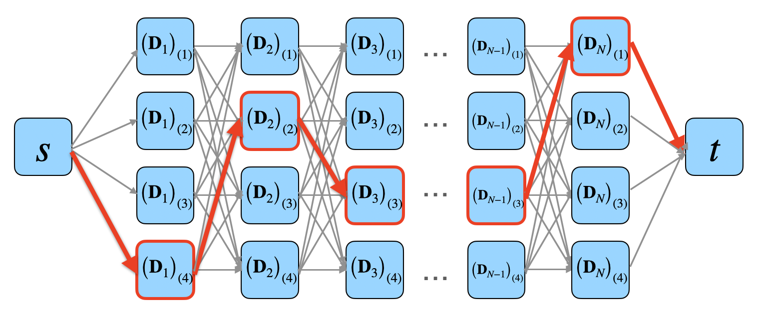
Figure 1: A schematic diagram for global_matching (Algorithm 2). At each iteration, we find the shortest path from $s$ to $t$ (highlighted with red), estimate one atom of $\mathbf{D}^{g*}$ using all passed vertices and remove the path (including the vertices) from $\mathcal{G}$.

The above optimization aims to obtain the appropriate signed permutation matrices $\{\mathbf{\Pi}_{i}\}_{i=1}^{N}$ that align the first $r^{g}$ atoms of the permuted dictionaries. In the ideal regime where $\mathbf{D}_{i}^{(0)}=\mathbf{D}_{i}^{*},1\leq i\leq N$, the optimal solution $\{\mathbf{\Pi}^{*}_{i}\}_{i=1}^{N}$ yields a zero objective value and satisfies $\left(\mathbf{D}_{i}^{(0)}\mathbf{\Pi}^{*}_{i}\right)_{(1:r^{g})}=\mathbf{D}^{g*}$. However, there are two main challenges with the above optimization. First, it is a nonconvex, combinatorial problem over the discrete sets $\{\mathcal{P}(r_{i})\}$. Second, the initial dictionaries may not coincide with their true counterparts. To address the first challenge, we show that the optimal solution to the optimization (7) can be efficiently obtained by solving a series of shortest path problems defined over an auxiliary graph. To alleviate the second challenge, we show that our proposed algorithm is robust against possible errors in the initial dictionaries.

Consider a weighted $N$-layered directed acyclic graph (DAG) $\mathcal{G}$ with $r_{i}$ nodes in layer $i$ representing the $r_{i}$ atoms in $\mathbf{D}_{i}$. We connect any node $a$ from layer $i$ to any node $b$ from layer $i+1$ with a directed edge with weight $w(a,b)=d_{2}\left(\left(\mathbf{D}_{i}\right)_{a},\left(\mathbf{D}_{i+1}\right)_{b}\right)$. We add a source node $s$ and connect it to all nodes in layer 1 with weight 0. Similarly, we include a terminal node $t$ and connect all nodes in layer $N$ to $t$ with weight 0. A schematic construction of this graph is presented in Figure 1. Given the constructed graph, Algorithm 2 aims to solve (7) by running $r^{g}$ rounds of the shortest path problem: at each round, the algorithm identifies the most aligned atoms in the initial dictionaries by obtaining the shortest path from $s$ to $t$. Then it removes the used nodes in the path for the next round. The correctness and robustness of the proposed algorithm are established in the next theorem.

Algorithm 2 global_matching

1:  Input: $\left\{\mathbf{D}^{(0)}_{i}\right\}_{i=1}^{N}$ and $r^{g}$.

2:  Construct the weighted $N$-layer DAG $\mathcal{G}$ described in Section 3.1.

3:  Initialize $\{\mathrm{index}_{i}\}_{i=1}^{N}$ as empty sets and $\mathbf{D}^{g,(0)}$ as an empty matrix.

4:  for $j=1,\dots,r^{g}$ do

5:     Find the shortest path $P=\left(s,(\mathbf{D}^{(0)}_{1})_{(\alpha_{1})},(\mathbf{D}^{(0)}_{1})_{(\alpha_{2})},\cdots,(\mathbf{D}^{(0)}_{N})_{(\alpha_{N})},t\right)$.

6:     Add $\frac{1}{N}\sum_{i=1}^{N}\mathrm{sign}\left(\left\langle(\mathbf{D}^{(0)}_{i})_{(\alpha_{i})},(\mathbf{D}^{(0)}_{1})_{(\alpha_{1})}\right\rangle\right)(\mathbf{D}^{(0)}_{i})_{(\alpha_{i})}$ as a new column of $\mathbf{D}^{g,(0)}$.

7:     Add $\alpha_{i}$ to $\mathrm{index}_{i}$ for every $i=1,\dots,N$.

8:     Remove $\mathcal{P}$ from $\mathcal{G}$.

9:  end for

10:  Set $\mathbf{D}_{i}^{l,(0)}=(\mathbf{D}^{(0)}_{i})_{([r_{i}]\setminus\mathrm{index}_{i})}$ for every $i=1,\dots,N$.

11:  return  $\left(\mathbf{D}^{g,(0)},\left\{\mathbf{D}_{i}^{l,(0)}\right\}_{i=1}^{N}\right)$.

Theorem 1 (Correctness and robustness of global_matching).

Suppose $\{\mathbf{D}^{*}_{i}\}_{i=1}^{N}$ are $\mu$-incoherent (Assumption 1) and $\beta$-identifiable (Assumption 2). Suppose the initial dictionaries $\left\{\mathbf{D}^{(0)}_{i}\right\}_{i=1}^{N}$ satisfy $d_{1,2}\left(\mathbf{D}^{(0)}_{i},\mathbf{D}^{*}_{i}\right)\leq\epsilon_{i}$ with $4\sum_{i=1}^{N}\epsilon_{i}\leq\min\left\{\sqrt{2-2\frac{\mu}{\sqrt{d}}},\beta\right\}$. Then, the output of Algorithm 2 satisfies:

$$d_{1,2}\left(\mathbf{D}^{g,(0)},\mathbf{D}^{g*}\right)\leq\frac{1}{N}\sum_{i=1}^{N}\epsilon_{i},\qquad\text{and}\qquad d_{1,2}\left(\mathbf{D}^{l,(0)}_{i},\mathbf{D}^{l*}_{i}\right)\leq\epsilon_{i},\quad\mathrm{for}\quad 1\leq i\leq N.$$ (8)

According to the above theorem, global_matching can robustly separate the clients’ initial dictionaries into global and local parts, provided that the aggregated error in the initial dictionaries is below a threshold. Specific initialization schemes that can satisfy the condition of Theorem 1 include Algorithm 1 from Agarwal et al., (2013) and Algorithm 3 from Arora et al., (2015). We also remark that since the constructed graph is a DAG, the shortest path problem can be solved in time linear in the number of edges, which is $\mathcal{O}\left(r_{1}+r_{N}+\sum_{i=1}^{N-1}r_{i}r_{i+1}\right)$, via a simple labeling algorithm (see, e.g., (Ahuja et al.,, 1988, Chapter 4.4)). Since we need to solve the shortest path problem $r^{g}$ times, this brings the computational complexity of Algorithm 2 to $\mathcal{O}(r^{g}Nr_{\max}^{2})$, where $r_{\max}=\max_{i}r_{i}$.

Given the initial local and global dictionaries, the clients progressively refine their estimates by applying $T$ rounds of local_update (Algorithm 3). At a high level, each client runs a single iteration of a linearly convergent algorithm $\mathcal{A}_{i}$ (see Definition 2), followed by an alignment step that determines the global atoms of the updated dictionary using $\mathbf{D}^{g,(t)}$ as a "reference point". Notably, our implementation of local_update is adaptive to different DL algorithms. This flexibility is indeed intentional to provide a versatile meta-algorithm for clients with different DL algorithms.

Algorithm 3 local_update

1:  Input: $\mathbf{D}^{(t)}_{i}=\left[\mathbf{D}^{g,(t)}\quad\mathbf{D}^{l,(t)}_{i}\right],\mathbf{Y}_{i}$

2:  $\mathbf{D}^{(t+1)}_{i}=\mathcal{A}_{i}\left(\mathbf{Y}_{i},\mathbf{D}^{(t)}_{i}\right)$ // One iteration of a linearly-convergent algorithm.

3:  Initialize $\mathcal{S}$ as an empty set and $\mathbf{P}\in\mathbb{R}^{r^{g}\times r^{g}}$ as an all-zero matrix.

4:  for $j=1,...,r^{g}$ do

5:     Find $k^{*}=\arg\min_{k}d_{2}\left(\left(\mathbf{D}^{g,(t)}\right)_{(j)},\left(\mathbf{D}^{(t+1)}_{i}\right)_{(k)}\right)$.

6:     Append $k^{*}$ to $\mathcal{S}$.

7:     Set $(i,i)$-th entry of $\mathbf{P}$ to $\mathrm{sign}\left(\left\langle\left(\mathbf{D}^{g,(t)}\right)_{(j)},\left(\mathbf{D}^{(t+1)}_{i}\right)_{(k^{*})}\right\rangle\right)$.

8:  end for

9:  Output: $\mathbf{D}^{g,(t+1)}_{i}=\left(\mathbf{D}^{(t+1)}_{i}\right)_{(\mathcal{S})}\mathbf{P}$ and $\mathbf{D}^{l,(t+1)}_{i}=\left(\mathbf{D}^{(t+1)}_{i}\right)_{([r_{i}]\setminus\mathcal{S})}$.

4 Theoretical Guarantees

In this section, we show that our proposed meta-algorithm provably solves $\mathsf{PerDL}$ under suitable initialization, identifiability, and algorithmic conditions. To achieve this goal, we first present the definition of a linearly-convergent DL algorithm.

Definition 2.

Given a generative model ${\mathbf{Y}}={\mathbf{D}}^{*}{\mathbf{X}}^{*}$, a DL algorithm $\mathcal{A}$ is called ${(\delta,\rho,\psi)}$-linearly convergent for some parameters $\delta,\psi>0$ and $0<\rho<1$ if, for any $\mathbf{D}\in\mathbb{R}^{d\times r}$ such that $d_{1,2}(\mathbf{D},\mathbf{D}^{*})\leq\delta$, the output of one iteration $\mathbf{D}^{+}=\mathcal{A}(\mathbf{D},{\mathbf{Y}})$, satisfies

$$d_{2,(j)}\left(\mathbf{D}^{+},\mathbf{D}^{*}\right)\leq\rho d_{2,(j)}\left(\mathbf{D},\mathbf{D}^{*}\right)+\psi,\quad\forall 1\leq j\leq r.$$ (9)

One notable linearly convergent algorithm is introduced by (Arora et al.,, 2015, Algorithm 5); we will discuss this algorithm in more detail in the appendix. Assuming all clients are equipped with linearly convergent algorithms, our next theorem establishes the convergence of $\mathsf{PerMA}$.

Theorem 2 (Convergence of $\mathsf{PerMA}$).

Suppose $\{\mathbf{D}^{*}_{i}\}_{i=1}^{N}$ are $\mu$-incoherent (Assumption 1) and $\beta$-identifiable (Assumption 2). Suppose, for every client $i$, the DL algorithm $\mathcal{A}_{i}$ used in local_update (Algorithm 3) is $(\delta_{i},\rho_{i},\psi_{i})$-linearly convergent with $4\sum_{i=1}^{N}\delta_{i}\leq\min\left\{\sqrt{2-2\frac{\mu}{\sqrt{d}}},\beta\right\}$. Assume the initial dictionaries $\{\mathbf{D}^{(0)}_{i}\}_{i=1}^{N}$ satisfy:

$$d_{1,2}\left(\frac{1}{N}\sum_{i=1}^{N}\mathbf{D}^{g,(0)}_{i},\mathbf{D}^{g*}\right)\leq\min_{1\leq i\leq N}\delta_{i},\quad d_{1,2}\left(\mathbf{D}^{l,(0)}_{i},\mathbf{D}^{l*}_{i}\right)\leq\delta_{i},\quad\text{for}\quad i=1,\dots,N.$$ (10)

Then, for every $t\geq 0$, $\mathsf{PerMA}$ (Algorithm 1) satisfies

$$d_{1,2}\left(\mathbf{D}^{g,(t+1)},\mathbf{D}^{g*}\right) \leq\left(\frac{1}{N}\sum_{i=1}^{N}\rho_{i}\right)d_{1,2}\left(\mathbf{D}^{g,(t)},\mathbf{D}^{g*}\right)+{\frac{1}{N}\sum_{i=1}^{N}\psi_{i}},$$ (11)

$$d_{1,2}\left(\mathbf{D}^{l,(t+1)}_{i},\mathbf{D}^{l*}_{i}\right) \leq\rho_{i}d_{1,2}\left(\mathbf{D}^{l,(t)},\mathbf{D}^{l*}_{i}\right)+{\psi_{i}},\quad\mathrm{for}\quad 1\leq i\leq N.$$ (12)

The above theorem sheds light on a number of key benefits of $\mathsf{PerMA}$:

Relaxed initial condition for weak clients.

Our algorithm relaxes the initial condition on the global dictionaries. In particular, it only requires the average of the initial global dictionaries to be close to the true global dictionary. Consequently, it enjoys a provable convergence guarantee even if some of the clients do not provide a high-quality initial dictionary to the server.

Improved convergence rate for slow clients.

During the course of the algorithm, the global dictionary error decreases at an average rate of $\frac{1}{N}\sum_{i=1}^{N}\rho_{i}$, improving upon the convergence rate of the slow clients.

Improved statistical error for weak clients.

A linearly convergent DL algorithm $\mathcal{A}_{i}$ stops making progress upon reaching a neighborhood around the true dictionary $\mathbf{D}_{i}^{*}$ with radius $O(\psi_{i})$. This type of guarantee is common among DL algorithms (Arora et al.,, 2015; Liang et al.,, 2022) and often corresponds to their statistical error. In light of this, $\mathsf{PerMA}$ improves the performance of weak clients (i.e., clients with weak statistical guarantees) by borrowing strength from strong ones.

5 Numerical Experiments

In this section, we showcase the effectiveness of Algorithm 1 using synthetic and real data. All experiments are performed on a MacBook Pro 2021 with the Apple M1 Pro chip and 16GB unified memory for a serial implementation in MATLAB 2022a. Due to limited space, we will only provide high-level motivation and implication of our experiments and defer implementation details to the appendix.

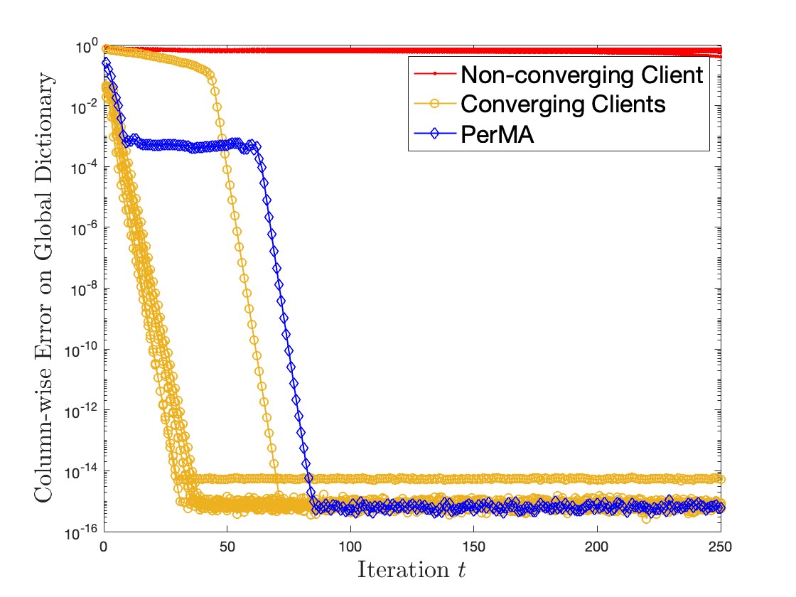
Figure 2: $\mathsf{PerMA}$ improves the accuracy of the recovered global dictionary for all clients, even if some (three out of ten) are weak learners.

5.1 Synthetic Dataset

In this section, we validate our theoretical results on a synthetic dataset. We consider ten clients, each with a dataset generated according to the model 1. The details of our construction are presented in the appendix. Specifically, we compare the performances of two strategies: (1) independent strategy, where each client solves DL without any collaboration, and (2) collaborative strategy, where clients collaboratively learn the ground truth dictionaries by solving $\mathsf{PerDL}$ via the proposed meta-algorithm $\mathsf{PerMA}$. We initialize both strategies using the same $\{\mathbf{D}^{(0)}_{i}\}_{i=1}^{N}$. The initial dictionaries are obtained via a warm-up method proposed in (Liang et al.,, 2022, Algorithm 4). For a fair comparison between independent and collaborative strategies, we use the same DL algorithm ((Liang et al.,, 2022, Algorithm 1)) for different clients. Note that in the independent strategy, the clients cannot separate global from local dictionaries. Nonetheless, to evaluate their performance, we collect the atoms that best align with the true global dictionary $\mathbf{D}^{g*}$ and treat them as the estimated global dictionaries. As can be seen in Figure 2, three out of ten clients are weak learners and fail to recover the global dictionary with desirable accuracy. On the contrary, in the collaborative strategy, all clients recover the same global dictionary almost exactly.

5.2 Training with Imbalanced Data

In this section, we showcase the application of $\mathsf{PerDL}$ in training with imbalanced datasets. We consider an image reconstruction task on MNIST dataset. This dataset corresponds to a set of handwritten digits (see the first row of Figure 3). The goal is to recover a single concise global dictionary that can be used to reconstruct the original handwritten digits as accurately as possible. In particular, we study a setting where the clients have imbalanced label distributions. Indeed, data imbalance can drastically bias the performance of the trained model in favor of the majority groups, while hurting its performance on the minority groups (Leevy et al.,, 2018; Thabtah et al.,, 2020). Here, we consider a setting where the clients have highly imbalanced datasets, where $90\%$ of their samples have the same label. More specifically, for client $i$, we assume that $90\%$ of the samples correspond to the handwritten digit “$i$”, with the remaining $10\%$ corresponding to other digits. The second row of Figure 3 shows the effect of data imbalance on the performance of the recovered dictionary on a single client, when the clients do not collaborate. The last row of Figure 3 shows the improved performance of the recovered dictionary via $\mathsf{PerDL}$ on the same client. Our experiment clearly shows the ability of $\mathsf{PerDL}$ to effectively address the data imbalance issue by combining the strengths of different clients.

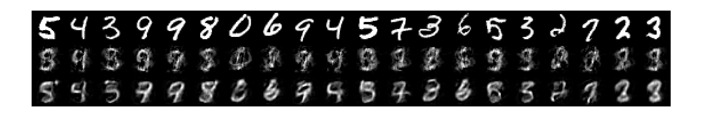
Figure 3: $\mathsf{PerMA}$ improves training with imbalanced datasets. We consider the image reconstruction task on the imbalanced MNIST dataset using only five atoms from a learned global dictionary. The first row corresponds to the original images. The second row is based on the dictionary learned on a single client with an imbalanced dataset. The third row shows the improved performance of the learned dictionary using our proposed method on the same client.

5.3 Surveillance Video Dataset

As a proof of concept, we consider a video surveillance task, where the goal is to separate the background from moving objects. Our data is collected from Cuevas et al., (2016) (see the first column of Figure 4). As these frames are taken from one surveillance camera, they share the same background corresponding to the global features we aim to extract. The frames also exhibit heterogeneity as moving objects therein are different from the background. This problem can indeed be modeled as an instance of $\mathsf{PerDL}$, where each video frame can be assigned to a “client”, with the global dictionary capturing the background and local dictionaries modeling the moving objects. We solve $\mathsf{PerDL}$ by applying $\mathsf{PerMA}$ to obtain a global dictionary and several local dictionaries for this dataset. Figure 4 shows the reconstructed background and moving objects via the recovered global and local dictionaries. Our results clearly show the ability of our proposed framework to separate global and local features.

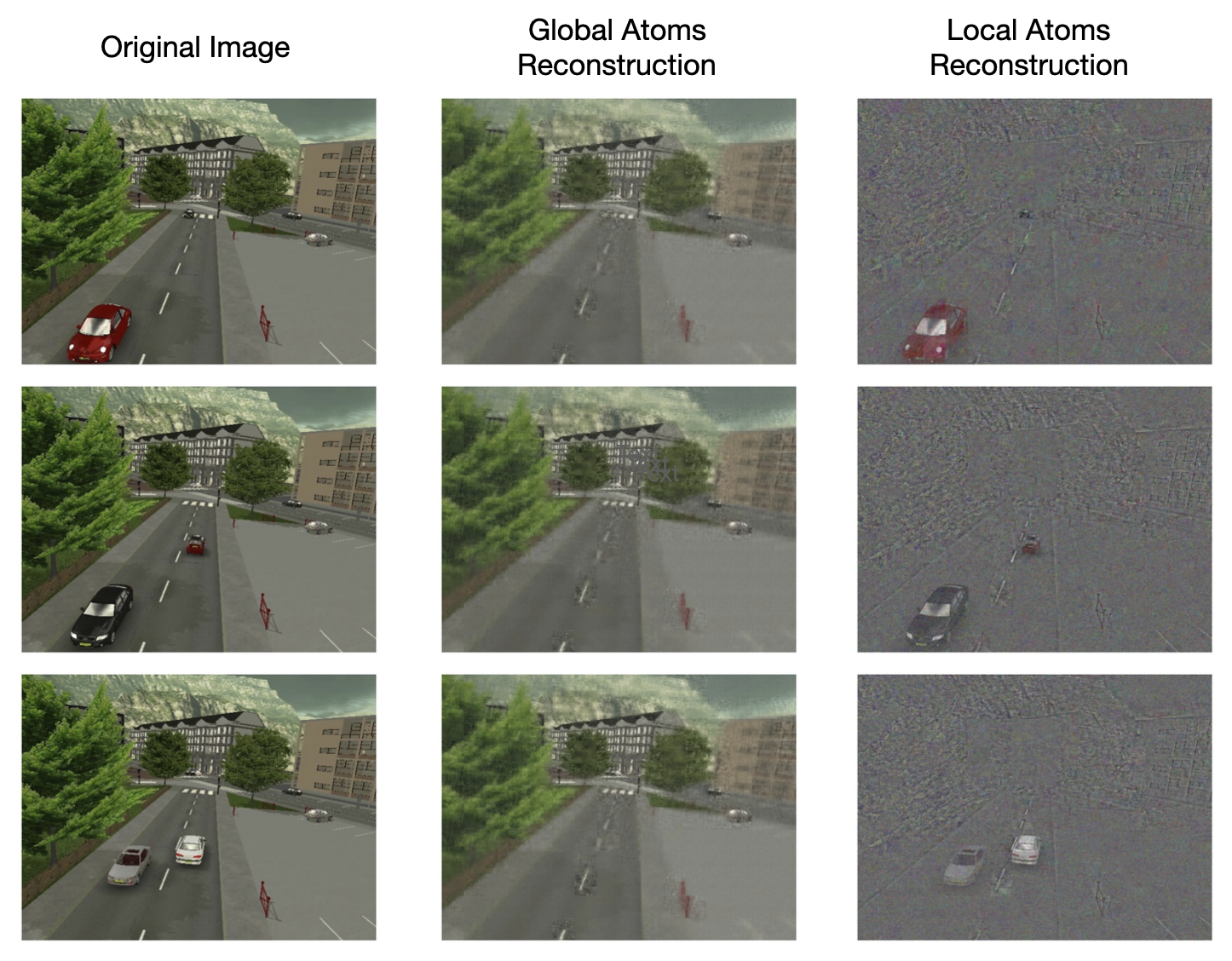
Figure 4: $\mathsf{PerMA}$ effectively separates the background from moving objects in video frames. Here we reconstruct the surveillance video frames using global and local dictionaries learned by $\mathsf{PerMA}$. We reconstruct the frames using only $50$ atoms from the combined dictionaries.

6 Conclusion and Future Directions

In this work, we introduce the problem of Personalized Dictionary Learning (PerDL), where the goal is to learn global and local dictionaries for heterogeneous datasets. One promising direction for future research is to relax the requirement on the linear convergence of the DL algorithm (Definition 2). Moreover, it would be worthwhile to investigate whether the convergence and statistical guarantees of our proposed algorithm can be improved beyond Theorem 2.

Appendix A Further Details on the Experiments

In this section, we provide further details on the numerical experiments reported in Section 5.

A.1 Details of Section 5.1

In Section 5.1, we generate the synthetic datasets according to Model 1 with $N=10$, $d=6$, $r_{i}=6$, and $n_{i}=200$ for each $1\leq i\leq 10$. Each $\mathbf{D}^{*}_{i}$ is an orthogonal matrix with the first $r^{g}=3$ columns shared with every other client and the last $r^{l}_{i}=3$ columns unique to themselves. Each $\mathbf{X}^{*}_{i}$ is first generated from a Gaussian-Bernoulli distribution where each entry is non-zero with a probability $0.2$. Then, $\mathbf{X}^{*}_{i}$ is further truncated, where all the entries $\left(\mathbf{X}^{*}_{i}\right)_{(j,k)}$ with $|\left(\mathbf{X}^{*}_{i}\right)_{(j,k)}|<0.3$ are replaced by $\left(\mathbf{X}^{*}_{i}\right)_{(j,k)}=0.3\times\mathrm{sign}(\left(\mathbf{X}^{*}_{i}\right)_{(j,k)})$.

We use the orthogonal DL algorithm (Algorithm 4) introduced in (Liang et al.,, 2022, Algorithm 1) as the local DL algorithm for each client. This algorithm is simple to implement and comes equipped with a strong convergence guarantee (see (Liang et al.,, 2022, Theorem 1)). Here $\mathrm{HT}_{\zeta}(\cdot)$ denotes the hard-thresholding operator at level $\zeta$, which is defined as:

$$\left(\mathrm{HT}_{\zeta}(\mathbf{A})\right)_{(i,j)}=\begin{cases}\mathbf{A}_{(i,j)}&\text{if}\quad|\mathbf{A}_{(i,j)}|\geq\zeta,\\ 0&\text{if}\quad|\mathbf{A}_{(i,j)}|<\zeta.\\ \end{cases}$$

Specifically, we use $\zeta=0.15$ for the experiments in Section 5.1. $\mathrm{Polar}(\cdot)$ denotes the polar decomposition operater, which is defined as $\mathrm{Polar}(\mathbf{A})=\mathbf{U}_{\mathbf{A}}\mathbf{V}_{\mathbf{A}}^{\top}$, where $\mathbf{U}_{\mathbf{A}}\mathbf{\Sigma}_{\mathbf{A}}\mathbf{V}_{\mathbf{A}}^{\top}$ is the Singular Value Decomposition (SVD) of $\mathbf{A}$.

Algorithm 4 Alternating minimization for orthogonal dictionary learning (Liang et al., (2022))

1:  Input: $\mathbf{Y}_{i}$, $\mathbf{D}^{(t)}_{i}$

2:  Set $\mathbf{X}^{(t)}_{i}=\mathrm{HT}_{\zeta}\left(\mathbf{D}^{(t)_{i}\top}\mathbf{Y}_{i}\right)$

3:  Set $\mathbf{D}^{(t+1)}_{i}=\mathrm{Polar}\left(\mathbf{Y}_{i}\mathbf{X}^{(t)\top}_{i}\right)$

4:  return  $\mathbf{D}^{(t+1)}_{i}$

For a fair comparison, we initialize both strategies using the same $\{\mathbf{D}^{(0)}_{i}\}_{i=1}^{N}$, which is obtained by iteratively calling Algorithm 4 with a random initial dictionary and shrinking thresholds $\zeta$. For a detailed discussion on such an initialization scheme we refer the reader to Liang et al., (2022).

A.2 Details of Section 5.2

In section 5.2, we aim to learn a dictionary with imbalanced data collected from MNIST dataset (LeCun et al.,, 2010). Specifically, we consider $N=10$ clients, each with $500$ handwritten images. Each image is comprised of $28\times 28$ pixels. Instead of randomly assigning images, we construct dataset $i$ such that it contains $450$ images of digit $i$ and $50$ images of other digits. Here client $10$ corresponds to digit $0$. After vectorizing each image into a $784\times 1$ one-dimension signal, our imbalanced dataset contains $10$ matrices $\mathbf{Y}_{i}\in\mathbb{R}^{784\times 500},i=1,\dots,10$.

We first use Algorithm 4 to learn an orthogonal dictionary for each client, using their own imbalanced dataset. For client $i$, given the output of Algorithm 4 after $T$ iterations $\mathbf{D}^{(T)}_{i}$, we reconstruct a new signal $\mathbf{y}$ using the top $k$ atoms according to the following steps: first, we solve a sparse coding problem to find the sparse code $\mathbf{x}$ such that $\mathbf{y}\approx\mathbf{D}^{(T)}_{i}\mathbf{x}$. This can be achieved by Step 2 in Algorithm 4. Second, we find the top $k$ entries in $\mathbf{x}$ that have the largest magnitude: $\mathbf{x}_{(\alpha_{1},1)}$, $\mathbf{x}_{(\alpha_{2},1)},\cdots,\mathbf{x}_{(\alpha_{k},1)}$. Finally, we calculate the reconstructed signal $\tilde{\mathbf{y}}$ as

$$\tilde{\mathbf{y}}=\sum_{j=1}^{k}\mathbf{x}_{(\alpha_{h},1)}\left(\mathbf{D}^{(T)}_{i}\right)_{\alpha_{h}}.$$

The second row of Figure 3 is generated by the above procedure with $k=5$ using the dictionary learned by Client $1$. The third row of Figure 3 corresponds to the reconstructed images using the output of $\mathsf{PerMA}$.

A.3 Details of Section 5.3

Our considered dataset in section 5.3 contains 62 frames, each of which is a $480\times 640\times 3$ RGB image. We consider each frame as one client ($N=62$). After dividing each frame into $40\times 40$ patches, we obtain each data matrix $\mathbf{Y}_{i}\in\mathbb{R}^{576\times 1600}$. Then we apply $\mathsf{PerMA}$ to $\{\mathbf{Y}_{i}\}_{i=1}^{62}$ with $r_{i}=576$ for all $i$ and $r^{g}=30$. Consider $\mathbf{D}^{(T)}_{i}=\left[\mathbf{D}^{g,(T)}\quad\mathbf{D}^{l,(T)}_{i}\right]$, which is the output of $\mathsf{PerMA}$ for client $i$. We reconstruct each $\mathbf{Y}_{i}$ using the procedure described in the previous section with $k=50$. Specifically, we separate the contribution of $\mathbf{D}^{g,(T)}$ from $\mathbf{D}^{l,(T)}_{i}$. Consider the reconstructed matrix $\tilde{Y}_{i}$ as

$$\tilde{\mathbf{Y}}_{i}=\begin{bmatrix}\mathbf{D}^{g,(T)}&\mathbf{D}^{l,(T)}_{i}\end{bmatrix}\begin{bmatrix}\mathbf{X}^{g}_{i}\\ \mathbf{X}^{l}_{i}\end{bmatrix}=\underbrace{\mathbf{D}^{g,(T)}\mathbf{X}^{g}_{i}}_{\tilde{\mathbf{Y}}_{i}^{g}}+\underbrace{\mathbf{D}^{l,(T)}_{i}\mathbf{X}^{l}_{i}}_{\tilde{\mathbf{Y}}_{i}^{l}}$$

The second column and the third column of Figure 4 correspond to reconstructed results of $\tilde{\mathbf{Y}}_{i}^{g}$ and $\tilde{\mathbf{Y}}_{i}^{l}$ respectively. We can see clear separation of the background (which is shared among all frames) from the moving objects (which is unique to each frame).

One notable difference between this experiment and the previous one is in the choice of the DL algorithm $\mathcal{A}_{i}$. To provide more flexibility, we relax the orthogonality condition for the dictionary. Therefore, we use the alternating minimization algorithm introduced in Arora et al., (2015) for each client (see Algorithm 5). The main difference between this algorithm and Algorithm 4 is that the polar decomposition step in Algorithm 4 is replaced by a single iteration of the gradient descent applied to the loss function $\mathcal{L}(\mathbf{D},\mathbf{X})=\|\mathbf{D}\mathbf{X}-\mathbf{Y}\|^{2}_{F}$.

Algorithm 5 Alternating minimization for general dictionary learning (Arora et al., (2015))

1:  Input: $\mathbf{Y}_{i}$, $\mathbf{D}^{(t)}_{i}$

2:  Set $\mathbf{X}^{(t)}_{i}=\mathrm{HT}_{\zeta}\left(\mathbf{D}^{(t)\top}_{i}\mathbf{Y}_{i}\right)$

3:  Set $\mathbf{D}^{(t+1)}_{i}=\mathbf{D}^{(t)}_{i}-2\eta\left(\mathbf{D}^{(t)}_{i}\mathbf{X}^{(t)}_{i}-\mathbf{Y}_{i}\right)\mathbf{X}^{(t)\top}_{i}$

4:  return  $\mathbf{D}^{(t+1)}_{i}$

Even with the computational saving brought up by Algorithm 5, the runtime significantly slows down for $\mathsf{PerMA}$ due to large $N$, $d$, and $p$. Here we report a practical trick to speed up $\mathsf{PerMA}$, which is a local refinement procedure (Algorithm 6) added immediately before local_update (Step 10 of Algorithm 1). At a high level, local_dictionary_refinement first finds the local residual data matrix $\mathbf{Y}^{l}_{i}$ by removing the contribution of the global dictionary. Then it iteratively refines the local dictionary with respect to $\mathbf{Y}^{l}_{i}$. We observed that local_dictionary_refinement significantly improves the local reconstruction quality. We leave its theoretical analysis as a possible direction for future work.

Algorithm 6 local_dictionary_refinement

1:  Input: $\mathbf{D}^{(t)}_{i}=\left[\mathbf{D}^{g,(t)}\quad\mathbf{D}^{l,(t)}_{i}\right],\mathbf{Y}_{i}$

2:  Find $\begin{bmatrix}\mathbf{X}^{g}_{i}\\ \mathbf{X}^{l}_{i}\end{bmatrix}$ such that $\mathbf{Y}_{i}\approx\left[\mathbf{D}^{g,(t)}\quad\mathbf{D}^{l,(t)}_{i}\right]\begin{bmatrix}\mathbf{X}^{g}_{i}\\ \mathbf{X}^{l}_{i}\end{bmatrix}$// Solving a sparse coding problem

3:  Set $\mathbf{Y}^{l}_{i}=\mathbf{Y}_{i}-\mathbf{D}^{g,(t)}\mathbf{X}^{g}_{i}$

4:  Set $\mathbf{D}^{\mathrm{refine},(0)}_{i}=\mathbf{D}^{l,(t)}_{i}$.

5:  for $\tau=0,1,...,T^{\mathrm{refine}}-1$ do

6:     Set $\mathbf{D}^{\mathrm{refine},(\tau+1)}_{i}=\mathcal{A}_{i}\left(\mathbf{Y}^{l}_{i},\mathbf{D}^{\mathrm{refine},(\tau)}_{i}\right)$ // Improving local dictionary

7:  end for

8:  return  $\mathbf{D}^{\mathrm{refine},(T^{\mathrm{refine}})}_{i}$ as refined $\mathbf{D}^{l,(t)}_{i}$

Appendix B Further Discussion on Linearly Convergent Algorithms

In this section, we discuss a linearly convergent DL algorithm that satisfies the conditions of our Theorem 2. In particular, the next theorem is adapted from (Arora et al.,, 2015, Theorem 12) and shows that a modified variant of Algorithm 5 introduced in (Arora et al.,, 2015, Algorithm 5) is indeed linearly-convergent.

Theorem 3 (Linear convergence of Algorithm 5 in Arora et al., (2015)).

Suppose that the data matrix satisfies $\mathbf{Y}=\mathbf{D}^{*}\mathbf{X}^{*}$, where $\mathbf{D}^{*}$ is an $\mu$-incoherent dictionary and the sparse code $\mathbf{X}^{*}$ satisfies the generative model introduced in Section 1.2 and Section 4.1 of Arora et al., (2015). For any initial dictionary $\|\mathbf{D}^{(0)}\|_{2}\leq 1$, Algorithm 5 in Arora et al., (2015) is $(\delta,\rho,\psi)$-linearly convergent with $\delta=O(1/\log d)$, $\rho\in(1/2,1)$, and $\psi=O(d^{-\omega(1)})$.

Algorithm 5 in Arora et al., (2015) is a refinement of Algorithm 5, where the error is further reduced by projecting out the components along the column currently being updated. For brevity, we do not discuss the exact implementation of the algorithm; an interested reader may refer to Arora et al., (2015) for more details. Indeed, we have observed in our experiments that the additional projection step does not provide a significant benefit over Algorithm 5.

Appendix C Proofs of Theorems

C.1 Proof of Theorem 1

To begin with, we establish a triangular inequality for $d_{1,2}(\cdot,\cdot)$, which will be important in our subsequent arguments:

Lemma 1 (Triangular inequality for $d_{1,2}(\cdot,\cdot)$).

For any dictionary $\mathbf{D}_{1}$, $\mathbf{D}_{2}$, $\mathbf{D}_{3}\in\mathbb{R}^{d\times r}$, we have

$$d_{1,2}\left(\mathbf{D}_{1},\mathbf{D}_{2}\right)\leq d_{1,2}\left(\mathbf{D}_{1},\mathbf{D}_{3}\right)+d_{1,2}\left(\mathbf{D}_{3},\mathbf{D}_{2}\right)$$ (13)

Proof.

Suppose $\mathbf{\Pi}_{1,3}$ and $\mathbf{\Pi}_{3,2}$ satisfy $d_{1,2}\left(\mathbf{D}_{1},\mathbf{D}_{3}\right)=\|\mathbf{D}_{1}\mathbf{\Pi}_{1,3}-\mathbf{D}_{3}\|_{1,2}$ and $d_{1,2}\left(\mathbf{D}_{3},\mathbf{D}_{2}\right)=\|\mathbf{D}_{3}-\mathbf{D}_{2}\mathbf{\Pi}_{3,2}\|_{1,2}$. Then we have

$$d_{1,2}\left(\mathbf{D}_{1},\mathbf{D}_{3}\right)+d_{1,2}\left(\mathbf{D}_{3},\mathbf{D}_{2}\right) =\|\mathbf{D}_{1}\mathbf{\Pi}_{1,3}-\mathbf{D}_{3}\|_{1,2}+\|\mathbf{D}_{3}-\mathbf{D}_{2}\mathbf{\Pi}_{3,2}\|_{1,2}$$ (14)

$$\geq\|\mathbf{D}_{1}\mathbf{\Pi}_{1,3}-\mathbf{D}_{2}\mathbf{\Pi}_{3,2}\|_{1,2}$$

$$\geq d_{1,2}\left(\mathbf{D}_{1},\mathbf{D}_{2}\right).$$

∎

Given how the directed graph $\mathcal{G}$ is constructed and modified, any directed path from $s$ to $t$ will be of the form $\mathcal{P}=s\rightarrow(\mathbf{D}^{(0)}_{1})_{\alpha(1)}\rightarrow(\mathbf{D}^{(0)}_{2})_{\alpha(2)}\rightarrow\cdots\rightarrow(\mathbf{D}^{(0)}_{N})_{\alpha(N)}\rightarrow t$. Specifically, each layer (or client) contributes exactly one node (or atom), and the path is determined by $\alpha(\cdot):[N]\rightarrow[r]$. Recall that $\mathbf{D}^{*}_{i}=\begin{bmatrix}\mathbf{D}^{g*}&\mathbf{D}^{l*}_{i}\end{bmatrix}$ for every $1\leq i\leq N$. Assume, without loss of generality, that for every client $1\leq i\leq N$,

$$\mathbf{I}_{r_{i}\times r_{i}}=\arg\min_{\mathbf{\Pi}\in\mathcal{P}(r_{i})}\left\|\mathbf{D}^{*}_{i}\mathbf{\Pi}-\mathbf{D}^{(0)}_{i}\right\|_{1,2}.$$ (15)

In other words, the first $r^{g}$ atoms in the initial dictionaries $\{D_{i}^{(0)}\}_{i=1}^{N}$ are aligned with the global dictionary. Now consider the special path $\mathcal{P}^{*}_{j}$ for $1\leq j\leq r^{g}$ defined as

$$\mathcal{P}^{*}_{j}=s\rightarrow(\mathbf{D}^{(0)}_{1})_{j}\rightarrow(\mathbf{D}^{(0)}_{2})_{j}\rightarrow\cdots\rightarrow(\mathbf{D}^{(0)}_{N})_{j}\rightarrow t.$$ (16)

To prove that Algorithm 2 correctly selects and aligns global atoms from clients, it suffices to show that $\{\mathcal{P}^{*}_{j}\}_{j=1}^{r^{g}}$ are the top-$r^{g}$ shortest paths from $s$ to $t$ in $\mathcal{G}$. The length of the path $\mathcal{P}^{*}_{j}$ can be bounded as

$$\mathcal{L}\left(\mathcal{P}^{*}_{j}\right) =\sum_{i=1}^{N-1}d_{2}\left((\mathbf{D}^{(0)}_{i})_{j},(\mathbf{D}^{(0)}_{i+1})_{j}\right)$$ (17)

$$=\sum_{i=1}^{N-1}\min\left\{\|(\mathbf{D}^{(0)}_{i})_{j}-(\mathbf{D}^{(0)}_{i+1})_{j}\|_{2},\|(\mathbf{D}^{(0)}_{i})_{j}+(\mathbf{D}^{(0)}_{i+1})_{j}\|_{2}\right\}$$

$$\leq\sum_{i=1}^{N-1}\|(\mathbf{D}^{(0)}_{i})_{j}-(\mathbf{D}^{(0)}_{i+1})_{j}\|_{2}$$

$$\leq\sum_{i=1}^{N-1}\|(\mathbf{D}^{(0)}_{i})_{j}-(\mathbf{D}^{g*})_{j}\|_{2}+\|(\mathbf{D}^{(0)}_{i+1})_{j}-(\mathbf{D}^{g*})_{j}\|_{2}$$

$$\leq\sum_{i=1}^{N-1}(\epsilon_{i}+\epsilon_{i+1})$$

$$\leq 2\sum_{i=1}^{N}\epsilon_{i}.$$

We move on to prove that all the other paths from $s$ to $t$ will have a distance longer than $2\sum_{i=1}^{N}\epsilon_{i}$. Consider a general directed path $\mathcal{P}=s\rightarrow(\mathbf{D}^{(0)}_{1})_{\alpha(1)}\rightarrow(\mathbf{D}^{(0)}_{2})_{\alpha(2)}\rightarrow\cdots\rightarrow(\mathbf{D}^{(0)}_{N})_{\alpha(N)}\rightarrow t$ that is not in $\{\mathcal{P}^{*}_{j}\}_{j=1}^{r^{g}}$. Based on whether or not $\mathcal{P}$ contains atoms that align with the true global ground atoms, there are two situations:

Case 1: Suppose there exists $1\leq i\leq N$ such that $\alpha(i)\leq r^{g}$. Given Model 1 and the assumed equality (15), we know that for layer $i$, $\mathcal{P}$ contains a global atom. Since $\mathcal{P}$ is not in $\{\mathcal{P}^{*}_{j}\}_{j=1}^{r^{g}}$, there must exist $k\neq i$ such that $\alpha(k)\neq\alpha(i)$. As a result, we have

$$\mathcal{L}(\mathcal{P}) \overset{(a)}{\geq}d_{1,2}\left((\mathbf{D}^{(0)}_{i})_{\alpha(i)},(\mathbf{D}^{(0)}_{k})_{\alpha(k)}\right)$$ (18)

$$\overset{(b)}{\geq}\min\left\{\|(\mathbf{D}^{*}_{i})_{\alpha(i)}-(\mathbf{D}^{*}_{k})_{\alpha(k)}\|_{2},(\mathbf{D}^{*}_{i})_{\alpha(i)}+(\mathbf{D}^{*}_{k})_{\alpha(k)}\|_{2}\right\}$$

$$\ \ \ \ \ -\|(\mathbf{D}^{*}_{i})_{\alpha(i)}-(\mathbf{D}^{(0)}_{i})_{\alpha(i)}\|_{2}-\|(\mathbf{D}^{*}_{k})_{\alpha(k)}-(\mathbf{D}^{(0)}_{k})_{\alpha(k)}\|_{2}$$

$$\overset{(c)}{\geq}\sqrt{2-2\left|\left\langle(\mathbf{D}^{*}_{k})_{\alpha(i)},(\mathbf{D}^{*}_{k})_{\alpha(k)}\right\rangle\right|}-2\max_{1\leq i\leq N}\epsilon_{i}$$

$$\overset{(d)}{\geq}\sqrt{2-2\frac{\mu}{\sqrt{d}}}-2\max_{1\leq i\leq N}\epsilon_{i}$$

$$\overset{(e)}{\geq}2\sum_{i=1}^{N}\epsilon^{g}_{i}$$

Here $(a)$ and $(b)$ are due to Lemma 1, $(c)$ is due to assumed equality (15), $(d)$ is due to the $\mu$-incoherency of $\mathbf{D}^{*}_{k}$, and finally $(e)$ is given by the assumption of Theorem 1.

Case 2: Suppose $\alpha(i)>r^{g}$ for all $1\leq i\leq N$, which means that the path $\mathcal{P}$ only uses approximations to local atoms. Consider the ground truth of these approximations, $(\mathbf{D}^{*}_{1})_{\alpha(1)},(\mathbf{D}^{*}_{2})_{\alpha(2)},...,(\mathbf{D}^{*}_{N})_{\alpha(N)}$. There must exist $1\leq i,j\leq N$ such that $d_{1,2}\left((\mathbf{D}^{*}_{i})_{\alpha(i)},(\mathbf{D}^{*}_{j})_{\alpha(j)}\right)\geq\beta$. Otherwise, it is easy to see that $\{\mathbf{D}^{l*}_{i}\}_{i=1}^{N}$ would not be $\beta$-identifiable because any $(\mathbf{D}^{*}_{i})_{\alpha(i)}$ will satisfy (6). As a result, we have the following:

$$\mathcal{L}(\mathcal{P}) \geq d_{1,2}\left((\mathbf{D}^{(0)}_{i})_{\alpha(i)},(\mathbf{D}^{(0)}_{j})_{\alpha(j)}\right)$$ (19)

$$\geq d_{1,2}\left((\mathbf{D}^{*}_{i})_{\alpha(i)},(\mathbf{D}^{*}_{j})_{\alpha(j)}\right)-\|(\mathbf{D}^{*}_{i})_{\alpha(i)}-(\mathbf{D}^{(0)}_{i})_{\alpha(i)}\|_{2}-\|(\mathbf{D}^{*}_{j})_{\alpha(j)}-(\mathbf{D}^{(0)}_{j})_{\alpha(j)}\|_{2}$$

$$\geq\beta-2\max_{i}\epsilon_{i}$$

$$\geq 2\sum_{i=1}^{N}\epsilon_{i}$$

So we have shown that $\{\mathcal{P}^{*}_{j}\}_{j=1}^{r^{g}}$ are the top-$r^{g}$ shortest paths from $s$ to $t$ in $\mathcal{G}$. Moreover, it is easy to show that $\mathrm{sign}\left(\left\langle(\mathbf{D}^{(0)}_{1})_{j},(\mathbf{D}^{(0)}_{i})_{j}\right\rangle\right)=1$ for small enough $\{\epsilon_{i}\}_{i=1}^{N}$. Therefore, the proposed algorithm correctly recovers the global dictionaries (with the correct identity permutation). Finally, we have $\mathbf{D}^{g,(0)}=\frac{1}{N}\sum_{i=1}^{N}(\mathbf{D}^{(0)}_{i})_{1:r^{g}}$, which leads to:

$$d_{1,2}\left(\mathbf{D}^{g,(0)},{\mathbf{D}}^{g*}\right) \leq\max_{1\leq j\leq r^{g}}\left\|\frac{1}{N}\sum_{i=1}^{N}(\mathbf{D}^{(0)}_{i})_{j}-(\mathbf{D}^{g*})_{j}\right\|_{2}$$ (20)

$$\leq\max_{1\leq j\leq r^{g}}\frac{1}{N}\sum_{i=1}^{N}\left\|(\mathbf{D}^{(0)}_{i})_{j}-(\mathbf{D}^{g*})_{j}\right\|_{2}$$

$$\leq\max_{1\leq j\leq r^{g}}\frac{1}{N}\sum_{i=1}^{N}\epsilon_{i}$$

$$=\frac{1}{N}\sum_{i=1}^{N}\epsilon_{i}.$$

This completes the proof of Theorem 1. $\hfill\square$

C.2 Proof of Theorem 2

Throughout this section, we define:

$$\bar{\rho}:=\frac{1}{N}\sum_{i=1}^{N}\rho_{i},\quad\quad\bar{\psi}:=\frac{1}{N}\sum_{i=1}^{N}\psi_{i}.$$ (21)

We will prove the convergence of the global dictionary in Theorem 2 by proving the following induction: at each $t\geq 1$, we have

$$d_{1,2}\left(\mathbf{D}^{g,(t+1)},\mathbf{D}^{g*}\right)\leq\bar{\rho}d_{1,2}\left(\mathbf{D}^{g,(t)},\mathbf{D}^{g*}\right)+\bar{\psi}.$$ (22)

At the beginning of communication round $t$, each client $i$ performs local_update to get $\mathbf{D}^{(t+1)}_{i}$ given $\left[\mathbf{D}^{g,(t)}\quad\mathbf{D}^{l,(t)}_{i}\right]$. Without loss of generality, we assume

$$\mathbf{I}_{r_{i}\times r_{i}} =\arg\min_{\mathbf{\Pi}\in\mathcal{P}(r_{i})}\left\|\mathbf{D}^{*}_{i}\mathbf{\Pi}-\left[\mathbf{D}^{g,(t)}\quad\mathbf{D}^{l,(t)}_{i}\right]\right\|_{1,2},$$ (23)

$$\mathbf{I}_{r_{i}\times r_{i}} =\arg\min_{\mathbf{\Pi}\in\mathcal{P}(r_{i})}\left\|\mathbf{D}^{*}_{i}\mathbf{\Pi}-\mathbf{D}^{(t+1)}_{i}\right\|_{1,2}.$$ (24)

Assumed equalities (23) and (24) imply that the permutation matrix that aligns the input and the output of $\mathcal{A}_{i}$ is also $\mathbf{I}_{r_{i}\times r_{i}}$. Specifically, the linear convergence property of $\mathcal{A}_{i}$ and Theorem 1 thus suggest:

$$\left\|\left(\mathbf{D}^{(t+1)}_{i}\right)_{j}-\left(\mathbf{D}^{*}_{i}\right)_{j}\right\|_{2}\leq\rho_{i}\left\|\left(\mathbf{D}^{g,(t)}\right)_{j}-\left(\mathbf{D}^{*}_{i}\right)_{j}\right\|_{2}+\psi_{i}\quad\forall 1\leq j\leq r^{g},1\leq i\leq N.$$ (25)

However, our algorithm is unaware of this trivial alignment. We will next show the remaining steps in local_update correctly recovers the identity permutation. The proof is very similar to the proof of Theorem 1 since we are essentially running Algorithm 2 on a two-layer $\mathcal{G}$. For every $1\leq i\leq N$, $1\leq j\leq r^{g}$, we have

$$d_{1,2}\left(\left(\mathbf{D}^{(t+1)}_{i}\right)_{j},\left(\mathbf{D}^{g,(t)}\right)_{j}\right) \leq d_{1,2}\left(\left(\mathbf{D}^{(t+1)}_{i}\right)_{j},\left(\mathbf{D}^{*}_{i}\right)_{j}\right)+d_{1,2}\left(\left(\mathbf{D}^{*}_{i}\right)_{j},\left(\mathbf{D}^{g,(t)}\right)_{j}\right)$$ (26)

$$\leq 2\delta_{i}.$$

Meanwhile for $k\neq j$,

$$d_{1,2}\left(\left(\mathbf{D}^{(t+1)}_{i}\right)_{k},\left(\mathbf{D}^{g,(t)}\right)_{j}\right)$$ (27)

$$\geq\ d_{1,2}\left(\left(\mathbf{D}^{*}_{i}\right)_{k},\left(\mathbf{D}^{*}_{i}\right)_{j}\right)-d_{1,2}\left(\left(\mathbf{D}^{(t+1)}_{i}\right)_{k},\left(\mathbf{D}^{*}_{i}\right)_{k}\right)-d_{1,2}\left(\left(\mathbf{D}^{*}_{i}\right)_{j},\left(\mathbf{D}^{g,(t)}\right)_{j}\right)$$

$$\geq\sqrt{2-\frac{2\mu}{\sqrt{d}}}-2\delta_{i}.$$

$$\geq 2\delta_{i}.$$

As a result, we successfully recover the identity permutation, which implies

$$\left\|\left(\mathbf{D}^{g,(t+1)}_{i}\right)_{j}-\left(\mathbf{D}^{g*}_{i}\right)_{j}\right\|_{2}\leq\rho_{i}\left\|\left(\mathbf{D}^{g,(t)}\right)_{j}-\left(\mathbf{D}^{g*}_{i}\right)_{j}\right\|_{2}+\psi_{i}\quad\forall 1\leq j\leq r^{g},1\leq i\leq N.$$ (28)

Finally, the aggregation step (Step 13 in Algorithm 1) gives:

$$d_{1,2}\left(\mathbf{D}^{g,(t+1)},\mathbf{D}^{g*}\right) \leq\left\|\frac{1}{N}\sum_{i=1}^{N}\mathbf{D}^{g,(t+1)}_{i}-\mathbf{D}^{g*}\right\|_{1,2}$$ (29)

$$=\max_{1\leq j\leq r^{g}}\left\|\left(\frac{1}{N}\sum_{i=1}^{N}\mathbf{D}^{g,(t+1)}_{i}\right)_{j}-\left(\mathbf{D}^{g*}\right)_{j}\right\|$$

$$\leq\max_{1\leq j\leq r^{g}}\frac{1}{N}\sum_{i=1}^{N}\left\|\left(\mathbf{D}^{g,(t+1)}_{i}\right)_{j}-\left(\mathbf{D}^{g*}_{i}\right)_{j}\right\|_{2}$$

$$\leq\max_{1\leq j\leq r^{g}}\frac{1}{N}\sum_{i=1}^{N}\left(\rho_{i}\left\|\left(\mathbf{D}^{g,(t)}\right)_{j}-\left(\mathbf{D}^{g*}_{i}\right)_{j}\right\|_{2}+\psi_{i}\right)$$

$$\leq\frac{1}{N}\sum_{i=1}^{N}\left(\rho_{i}d_{1,2}\left(\mathbf{D}^{g,(t)},\mathbf{D}^{g*}\right)+\psi_{i}\right)$$

$$=\bar{\rho}d_{1,2}\left(\mathbf{D}^{g,(t)},\mathbf{D}^{g*}\right)+\bar{\psi}.$$

As a result, we prove the induction (22) for all $0\leq t\leq T-1$. Inequality (12) is a by-product of the accurate separation of global and local atoms and can be proved by similar arguments. The proof is hence complete. $\hfill\square$

References

• Agarwal et al., (2016) Agarwal, A., Anandkumar, A., Jain, P., and Netrapalli, P. (2016). Learning sparsely used overcomplete dictionaries via alternating minimization. SIAM Journal on Optimization, 26(4):2775–2799.
• Agarwal et al., (2013) Agarwal, A., Anandkumar, A., and Netrapalli, P. (2013). Exact recovery of sparsely used overcomplete dictionaries. stat, 1050:8–39.
• Ahuja et al., (1988) Ahuja, R. K., Magnanti, T. L., and Orlin, J. B. (1988). Network flows.
• Arora et al., (2015) Arora, S., Ge, R., Ma, T., and Moitra, A. (2015). Simple, efficient, and neural algorithms for sparse coding. In Conference on learning theory, pages 113–149. PMLR.
• Arora et al., (2014) Arora, S., Ge, R., and Moitra, A. (2014). New algorithms for learning incoherent and overcomplete dictionaries. In Conference on Learning Theory, pages 779–806. PMLR.
• Bhagoji et al., (2019) Bhagoji, A. N., Chakraborty, S., Mittal, P., and Calo, S. (2019). Analyzing federated learning through an adversarial lens. In International Conference on Machine Learning, pages 634–643. PMLR.
• Chatterji and Bartlett, (2017) Chatterji, N. and Bartlett, P. L. (2017). Alternating minimization for dictionary learning with random initialization. Advances in Neural Information Processing Systems, 30.
• Cuevas et al., (2016) Cuevas, C., Yáñez, E. M., and García, N. (2016). Labeled dataset for integral evaluation of moving object detection algorithms: Lasiesta. Computer Vision and Image Understanding, 152:103–117.
• Fattahi and Sojoudi, (2020) Fattahi, S. and Sojoudi, S. (2020). Exact guarantees on the absence of spurious local minima for non-negative rank-1 robust principal component analysis. Journal of machine learning research.
• Fuchs, (2005) Fuchs, J.-J. (2005). Recovery of exact sparse representations in the presence of bounded noise. IEEE Transactions on Information Theory, 51(10):3601–3608.
• Ge et al., (2017) Ge, R., Jin, C., and Zheng, Y. (2017). No spurious local minima in nonconvex low rank problems: A unified geometric analysis. In International Conference on Machine Learning, pages 1233–1242. PMLR.
• Gkillas et al., (2022) Gkillas, A., Ampeliotis, D., and Berberidis, K. (2022). Federated dictionary learning from non-iid data. In 2022 IEEE 14th Image, Video, and Multidimensional Signal Processing Workshop (IVMSP), pages 1–5. IEEE.
• Huang et al., (2022) Huang, K., Liu, X., Li, F., Yang, C., Kaynak, O., and Huang, T. (2022). A federated dictionary learning method for process monitoring with industrial applications. IEEE Transactions on Artificial Intelligence.
• Karimireddy et al., (2020) Karimireddy, S. P., Kale, S., Mohri, M., Reddi, S., Stich, S., and Suresh, A. T. (2020). Scaffold: Stochastic controlled averaging for federated learning. In International Conference on Machine Learning, pages 5132–5143. PMLR.
• Kasiviswanathan et al., (2012) Kasiviswanathan, S., Wang, H., Banerjee, A., and Melville, P. (2012). Online l1-dictionary learning with application to novel document detection. Advances in neural information processing systems, 25.
• Kontar et al., (2017) Kontar, R., Zhou, S., Sankavaram, C., Du, X., and Zhang, Y. (2017). Nonparametric-condition-based remaining useful life prediction incorporating external factors. IEEE Transactions on Reliability, 67(1):41–52.
• LeCun et al., (2010) LeCun, Y., Cortes, C., Burges, C., et al. (2010). Mnist handwritten digit database.
• Leevy et al., (2018) Leevy, J. L., Khoshgoftaar, T. M., Bauder, R. A., and Seliya, N. (2018). A survey on addressing high-class imbalance in big data. Journal of Big Data, 5(1):1–30.
• Li et al., (2011) Li, S., Fang, L., and Yin, H. (2011). An efficient dictionary learning algorithm and its application to 3-d medical image denoising. IEEE transactions on biomedical engineering, 59(2):417–427.
• Li et al., (2021) Li, T., Hu, S., Beirami, A., and Smith, V. (2021). Ditto: Fair and robust federated learning through personalization. International Conference on Machine Learning.
• Liang et al., (2022) Liang, G., Zhang, G., Fattahi, S., and Zhang, R. Y. (2022). Simple alternating minimization provably solves complete dictionary learning. arXiv preprint arXiv:2210.12816.
• Liang et al., (2020) Liang, P. P., Liu, T., Ziyin, L., Allen, N. B., Auerbach, R. P., Brent, D., Salakhutdinov, R., and Morency, L.-P. (2020). Think locally, act globally: Federated learning with local and global representations. arXiv preprint arXiv:2001.01523.
• McMahan et al., (2017) McMahan, B., Moore, E., Ramage, D., Hampson, S., and y Arcas, B. A. (2017). Communication-efficient learning of deep networks from decentralized data. In Artificial Intelligence and Statistics, pages 1273–1282. PMLR.
• Meinshausen and Bühlmann, (2006) Meinshausen, N. and Bühlmann, P. (2006). High-dimensional graphs and variable selection with the lasso. Annals of Statistics.
• Ramirez et al., (2010) Ramirez, I., Sprechmann, P., and Sapiro, G. (2010). Classification and clustering via dictionary learning with structured incoherence and shared features. In 2010 IEEE Computer Society Conference on Computer Vision and Pattern Recognition, pages 3501–3508. IEEE.
• Ravishankar et al., (2020) Ravishankar, S., Ma, A., and Needell, D. (2020). Analysis of fast structured dictionary learning. Information and Inference: A Journal of the IMA, 9(4):785–811.
• Shi and Kontar, (2022) Shi, N. and Kontar, R. A. (2022). Personalized pca: Decoupling shared and unique features. arXiv preprint arXiv:2207.08041.
• Spielman et al., (2012) Spielman, D. A., Wang, H., and Wright, J. (2012). Exact recovery of sparsely-used dictionaries. In Conference on Learning Theory, pages 37–1. JMLR Workshop and Conference Proceedings.
• Sun et al., (2016) Sun, J., Qu, Q., and Wright, J. (2016). Complete dictionary recovery over the sphere i: Overview and the geometric picture. IEEE Transactions on Information Theory, 63(2):853–884.
• T Dinh et al., (2020) T Dinh, C., Tran, N., and Nguyen, J. (2020). Personalized federated learning with moreau envelopes. Advances in Neural Information Processing Systems, 33:21394–21405.
• Thabtah et al., (2020) Thabtah, F., Hammoud, S., Kamalov, F., and Gonsalves, A. (2020). Data imbalance in classification: Experimental evaluation. Information Sciences, 513:429–441.
• Tošić and Frossard, (2011) Tošić, I. and Frossard, P. (2011). Dictionary learning. IEEE Signal Processing Magazine, 28(2):27–38.
• Tropp, (2006) Tropp, J. A. (2006). Just relax: Convex programming methods for identifying sparse signals in noise. IEEE transactions on information theory, 52(3):1030–1051.
• Wang et al., (2020) Wang, H., Yurochkin, M., Sun, Y., Papailiopoulos, D., and Khazaeni, Y. (2020). Federated learning with matched averaging. arXiv preprint arXiv:2002.06440.
• Yazdi and Bouwmans, (2018) Yazdi, M. and Bouwmans, T. (2018). New trends on moving object detection in video images captured by a moving camera: A survey. Computer Science Review, 28:157–177.
• Yue et al., (2022) Yue, X., Nouiehed, M., and Al Kontar, R. (2022). Gifair-fl: A framework for group and individual fairness in federated learning. INFORMS Journal on Data Science.
• Zhao and Yu, (2006) Zhao, P. and Yu, B. (2006). On model selection consistency of lasso. The Journal of Machine Learning Research, 7:2541–2563.
• Zhao et al., (2021) Zhao, R., Li, H., and Liu, X. (2021). A survey of dictionary learning in medical image analysis and its application for glaucoma diagnosis. Archives of Computational Methods in Engineering, 28(2):463–471.