Mean field type control with species dependent dynamics
via structured tensor optimization

Abstract

In this work we consider mean field type control problems with multiple species that have different dynamics. We formulate the discretized problem using a new type of entropy-regularized multimarginal optimal transport problems where the cost is a decomposable structured tensor. A novel algorithm for solving such problems is derived, using this structure and leveraging recent results in entropy-regularized optimal transport. The algorithm is then demonstrated on a numerical example in robot coordination problem for search and rescue, where three different types of robots are used to cover a given area at minimal cost.

I Introduction

In recent years, mean field type control problems have emerged as a powerful tool for analysis and control of large-scale dynamical systems consisting of subsystem that are also dynamical systems. It provides a framework for modeling the behavior of a large population of interacting agents, where i) each individual’s decision is negligible to others at the individual level, but where the actions are significant when aggregated, and ii) the number of agents is too large to model each one individually. In such cases, one instead often seek a model that explains the aggregate behavior of the population [30, 32, 29, 17]. Mean field type control problems are density optimal control problems where the density abides to a controlled Fokker-Planck equation with distributed control [32, 10, 7, 13]. For example, potential mean field games are a particular type of such models [32, 6].

In basic formulations of mean field type control problems, all agents are equivalent in the sense that they all have the same dynamics and they all have the same objective function which they try to minimize. However, an important generalization is the multispecies setting, where the population consists of several different types of agents [30, 32, 31, 1, 15, 8]. This type of problem occurs in, e.g., coordination of multiple types of robots, where the robots have different properties (such as movement speed, movement capabilities, cost, etc.), but they still have a common goal of achieving a given task as efficiently as possible.

Recently optimal transport has been successfully used to address a number of problems in control, see, e.g., [9, 42, 45]. In the seminal paper [4], certain optimal transport problems were formulated as density control problems over the continuity equation, and this idea can be generalized to allow for optimal transport problems that have general underlying dynamics [28, 12]. Moreover, the recently developed Sinkhorn method, for numerically solving large-scale optimal transport problems [16, 37], is closely related to the density control formulation in [4]. In fact, the added entropy regularization leading to the Sinkhorn method corresponds to adding a stochastic term to the underlying particle dynamics, which leads to a controlled Fokker–Planck equation in the density control problem [11, 14]. This has been used to develop methods for solving potential mean field games [6, 38, 39], by formulating the potential mean field game as a mean field type control problem and then formulated the latter as a multimarginal optimal transport problem. Due to the Markov property, such multimarginal optimal transport problems have a graph-structured cost, and this type of graph structures has also been used to develop efficient computational methods to solve problems in control [23, 25], estimation [24], and information fusion [18].

In this paper, we consider mean field type control problems with multiple species that have different dynamics. First, we reformulate the problem as a multimarginal optimal transport problem. However, in this case the resulting problem turns out to have a cost function that is no longer graph-structured; instead, the cost function is a decomposable structured tensor, i.e., a multi-indexed matrix, which can be represented by a hypergraph. Next, for this type of structured multimarginal optimal transport problem, we develop an efficient solution algorithm. Finally, we illustrate the developed method on an example in coordination of multiple types of robots in a search-and-rescue type mission.

The outline of the paper is as follows: in Section II we briefly review the areas of multimarginal optimal transport, and mean field control problems. In Section III we formulate the multispecies mean field control problem as a structured multimarginal optimal transport problems, discretize it, and present an efficient numerical method for computing the optimal solution of the latter. In Section IV we present a detailed numerical example of robot coordination, and finally in Section V we present conclusions and future directions.

II Background

II-A Multimarginal optimal transport

The optimal transport problem is a classic problem in mathematics that involves finding the most efficient way of moving mass to transform one distribution into another [44]. The multimarginal optimal transport problem is an extension of this concept that deals with multiple distributions [40, 22, 36, 5]. Here, we focus on the discrete case, where the marginal distributions are represented by a finite set of nonnegative vectors $\mu_{1},\ldots,\mu_{\mathcal{T}}\in{\mathbb{R}}^{N}_{+}$. The transport plan and cost are both represented by ${\mathcal{T}}$-mode tensors, ${\bf M}\in{{\mathbb{R}}^{N^{\mathcal{T}}}}$ and ${\bf C}\in{{\mathbb{R}}^{N^{\mathcal{T}}}}$, respectively, and the marginal distributions of the transport plan are given by projections $P_{j}({\bf M})\in{\mathbb{R}}^{N}_{+}$, where

$$(P_{j}({\bf M}))_{i_{j}}:=\sum_{i_{1}=1}^{N}\cdots\sum_{i_{j-1}=1}^{N}\sum_{i_{j+1}=1}^{N}\cdots\sum_{i_{{\mathcal{T}}}=1}^{N}{\bf M}_{i_{1}\ldots i_{\mathcal{T}}}.$$

The discrete multimarginal optimal transport problem can then be formulated as

$$\underset{{\bf M}\in{\mathbb{R}}^{N^{{\mathcal{T}}}}_{+}}{\text{minimize }} \quad\langle{\bf C},{\bf M}\rangle$$ (1a)

subject to $$\quad P_{j}({\bf M})=\mu_{j},\;j\in\Gamma,$$ (1b)

where $\langle{\bf C},{\bf M}\rangle:=\sum_{i_{1},\ldots,i_{\mathcal{T}}}{\bf C}_{i_{1}\ldots i_{\mathcal{T}}}{\bf M}_{i_{1}\ldots i_{\mathcal{T}}}$ is the standard inner product, and where we impose constraints on the marginals corresponding to the index set $\Gamma\subset\{1,\ldots,{\mathcal{T}}\}$. Although the optimal transport problem (1) is a linear program, it can be challenging to solve it numerically due to the large number of variables. A popular method for approximately solving (1) is to perturb the problem by adding a small $\epsilon>0$ times the entropy term

$$D({\bf M}):=\sum_{i_{1},\ldots,i_{\mathcal{T}}}\big{(}{\bf M}_{i_{1}\ldots i_{\mathcal{T}}}\log({\bf M}_{i_{1}\ldots i_{\mathcal{T}}})-{\bf M}_{i_{1}\ldots i_{\mathcal{T}}}+1\big{)}$$

to the cost function and use Sinkhorn iterations to solve the resulting problem [16, 37]. The optimal transport plan for the perturbed problem is of the form ${\bf M}={\bf K}\odot{\bf U}$, where ${\bf K}=\exp(-{\bf C}/\epsilon)$, and ${\bf U}_{i_{1}\dots i_{\mathcal{T}}}=\prod_{j\in\Gamma}(u_{j})_{i_{j}}$ a rank-one tensor, see [5, 18]. Sinkhorn’s method iteratively updates $u_{j}$ as

$$u_{j}\leftarrow u_{j}\odot\mu_{j}\oslash P_{j}({\bf K}\odot{\bf U}),\quad\text{ for }j\in\Gamma,$$ (2)

where $\odot$ and $\oslash$ means pointwise multiplication and pointwise division, respectively, and the algorithm converges (linearly) to an optimal solution of the perturbed problem [35, 43]. In the multimarginal case, computing $P_{j}({\bf K}\odot{\bf U})$ suffers from the curse of dimensionality. However, in some cases, structures in the underlying cost ${\bf C}$ can be used to circumvent these issues, for instance when the cost decouples into pairwise interactions according to a graph-structure [5, 24, 23, 18, 25, 26, 27, 41, 2, 38, 39, 19].

II-B Multispecies mean field control problems

Consider a set of infinitesimal agents moving in a state space $X\subset{\mathbb{R}}^{n}$. Assume that they belong to $L$ different classes, and that each infinitesimal agent of species $\ell\in\{1,\ldots,L\}$ obeys the dynamics

$$dx_{\ell}(t)=f_{\ell}(x_{\ell})dt+B_{\ell}(x_{\ell})\big{(}v_{\ell}dt+\sqrt{\epsilon}dw_{\ell}\big{)},$$ (3)

subject to the initial condition $x_{\ell}(0)=x_{0,\ell}$, where the latter is a realization from a distribution $\rho_{0,\ell}(x)$. Moreover, $w_{\ell}$, for $\ell\in\{1,\ldots,L\}$, are $n$-dimensional Wiener processes that are independent of each other. We also assume that $f_{\ell}:X\to{\mathbb{R}}^{n}$ and $B_{\ell}:X\to{\mathbb{R}}^{n\times n}$ are continuously differentiable with bounded derivatives. Then, under suitable conditions on the (Markovian) feedback $v_{\ell}$, there exists a unique solution almost surely to (3), cf. [20, Thm. V.4.1], [7, pp. 7-8]. Moreover, the density of the particles of species $\ell$, $\rho_{\ell}$, is the solution of a controlled Fokker-Planck equation. Therefore, the multispecies mean field control problem is defined as the density optimal control problem

$$\underset{\begin{subarray}{c}\rho,\rho_{\ell},v_{\ell}\end{subarray}}{\text{minimize }} \;\int_{0}^{1}\!\!\!\int_{X}\sum_{\ell=1}^{L}\frac{1}{2}\|v_{\ell}\|^{2}\rho_{\ell}\,dxdt$$

$$+\!\int_{0}^{1}\!\!\mathcal{F}_{t}(\rho(t,\cdot))dt+\mathcal{G}(\rho(1,\cdot))$$ (4a)

$$+\sum_{\ell=1}^{L}\left(\int_{0}^{1}\mathcal{F}^{\ell}_{t}(\rho_{\ell}(t,\cdot))dt+\mathcal{G}^{\ell}(\rho_{\ell}(1,\cdot))\right)$$

subject to $$\;\frac{\partial\rho_{\ell}}{\partial t}+\nabla\cdot((f_{\ell}+B_{\ell}v_{\ell})\rho_{\ell})$$ (4b)

$$\quad-\frac{\epsilon}{2}\sum_{i,k=1}^{n}\frac{\partial^{2}((\sigma_{\ell})_{ik}\rho_{\ell})}{\partial x_{i}\partial x_{k}}=0,\quad\ell=1,\ldots L,$$

$$\;\rho_{\ell}(0,\cdot)=\rho_{0,\ell},\quad\rho(t,\cdot)=\sum_{\ell=1}^{L}\rho_{\ell}(t,\cdot),$$ (4c)

cf. [7, Chp. 2 and 4]. Here $\nabla\cdot$ denotes the divergence operator, $\sigma_{\ell}:=B_{\ell}B_{\ell}^{T}$, and $\mathcal{F}_{t}$, $\mathcal{G}$, $\mathcal{F}^{\ell}_{t}$ and $\mathcal{G}^{\ell}$ are functionals on on $L_{2}\cap L_{\infty}$. These functionals are the costs that the species are trying to minimize by their behavior: $\mathcal{F}^{\ell}_{t}$ and $\mathcal{G}^{\ell}$ are species-dependent costs, where the former is the running cost and the latter is the terminal cost. $\mathcal{F}_{t}$ and $\mathcal{G}$ are cooperative costs that link the species together by acting on the total density of all species. We assume that all these functionals are proper, convex, and lower-semicontinuous. Moreover, we assume that $\mathcal{F}_{t}$ and $\mathcal{F}^{\ell}_{t}$ are piece-wise continuous in time.

III Discretization and solution via tensor optimization

Recently, an approach for solving some types of potential mean field games was proposed in [38, 39]. The approach is based on formulating the problem on path space, i.e., on $C([0,1],X):=$ the set of continuous functions from $[0,1]$ to $X$, and then discretizing the problem in time and space, which results in a tensor optimization problem. Here we generalize this approach in order to derive a numerical solution algorithm for multispecies mean field control problems of the form (4).

III-A Discretization of the problem

Let ${\mathcal{P}}^{v_{\ell}}$ denote the distribution of species $\ell$ on path space, induced by the controlled process (3). Then ${\mathcal{P}}^{v_{\ell}}_{t}=\rho_{\ell}(t,\cdot)$, where ${\mathcal{P}}^{v_{\ell}}_{t}$ is the marginal of ${\mathcal{P}}^{v_{\ell}}$ corresponding to time $t$, and $\rho_{\ell}$ is the solution to (4b) with initial condition $\rho_{\ell}(0,\cdot)=\rho_{0,\ell}$. Moreover, let ${\mathcal{P}}^{0}_{\ell}$ denote the corresponding uncontrolled process ($v_{\ell}\equiv 0$) with initial density $\rho_{0,\ell}$. By the Girsanov theorem (see, e.g., [21, pp. 156-157]), we get that

$$\frac{1}{2}\int_{X}\int_{0}^{1}\!\!\|v_{\ell}\|^{2}\rho_{\ell}dtdx=\epsilon{\rm KL}({\mathcal{P}}^{v_{\ell}}\|{\mathcal{P}}^{0}_{\ell})$$ (5)

where ${\rm KL}(\cdot\|\cdot)$ is the Kullback-Leibler divergence, see, e.g., [11, 13, 6, 33, 34]. Utilizing (5), problem (4) can be reformulated as an optimization problem over path space measures that corresponds to a generalized entropy-regularized multimarginal optimal transport problem, see [38, 39]. In particular, discretizing the space into points $x_{1},\dots,x_{N}$, and considering time steps $j\Delta t$, for $j=1,\dots,{\mathcal{T}}$, where $\Delta t=1/{\mathcal{T}}$, the term (5) takes the form $\langle{\bf C}_{\ell},{\bf M}_{\ell}\rangle+\epsilon D({\bf M}_{\ell})$, where the tensor ${\bf M}_{\ell}\in{\mathbb{R}}^{N^{{\mathcal{T}}+1}}$ describes the flow of agents in class $\ell$, and the cost tensor ${\bf C}_{\ell}\in{\mathbb{R}}^{N^{{\mathcal{T}}+1}}$ describes the associated cost of moving agents. More precisely, $({\bf C}_{\ell})_{i_{0}\ldots i_{{\mathcal{T}}}}=\sum_{j=0}^{{\mathcal{T}}-1}C_{\ell i_{j}i_{j+1}}$, where $C_{\ell ik}$ is the optimal cost for moving a unit mass of species $\ell$ from point $x_{i}$ to $x_{k}$ in one time step, i.e.,

$$C_{\ell ik}\;=\;\begin{cases}\displaystyle\;\underset{v\in L_{2}([0,\Delta t])}{\text{minimize }}&\;\displaystyle\int_{0}^{\Delta t}\frac{1}{2}\|v\|^{2}dt\\ \;\text{subject to }&\;\displaystyle\dot{x}=f_{\ell}(x)+B_{\ell}(x)v\\ &\;\displaystyle x(0)=x_{i},\quad x(\Delta t)=x_{k}.\end{cases}$$ (6)

Thus, the discretization of (4) takes the form

$$\!\!\!\!\!\underset{\begin{subarray}{c}{\bf M}_{\ell},\mu_{j},\mu_{j}^{(\ell)}\\ j=1,\ldots,{\mathcal{T}}\\ \ell=1,\ldots,L\end{subarray}}{\text{minimize }} \,\sum_{\ell=1}^{L}\big{(}\langle{\bf C}_{\ell},{\bf M}_{\ell}\rangle+\epsilon D({\bf M}_{\ell})\big{)}+\Delta t\sum_{j=1}^{{\mathcal{T}}-1}F_{j}(\mu_{j})$$

$$+\!G(\mu_{\mathcal{T}})\!+\!\sum_{\ell=1}^{L}\!\!\left(\!\Delta t\!\sum_{j=1}^{{\mathcal{T}}-1}\!F_{j}^{\ell}(\mu_{j}^{(\ell)})\!+\!G^{\ell}(\mu_{\mathcal{T}}^{(\ell)})\!\right)$$ (7a)

subject to $$\,P_{j}({\bf M}_{\ell})=\mu_{j}^{(\ell)},\,j=1,\ldots,{\mathcal{T}},\,\ell=1,\ldots,L,$$ (7b)

$$\,P_{0}({\bf M}_{\ell})=\mu_{0,\ell},\;\ell=1,\ldots,L,$$ (7c)

$$\,\sum_{\ell=1}^{L}\mu_{j}^{(\ell)}=\mu_{j},\;\;\;j=0,\ldots,{\mathcal{T}}$$ (7d)

where $\mu_{0,\ell}$ are discrete approximations of $\rho_{0,\ell}$.

III-B Solution method based on tensor optimization

Note that (7) consists of $L$ coupled tensor optimization problems as in [38], which are coupled through the constraint (7d) and the cost imposed on $\mu_{j}$, for $j=1,\ldots,{\mathcal{T}}$, in (7a). Next, we reformulate (7) into a single tensor optimization problem (cf. [39, 26]) by “stacking together” the tensors ${\bf M}_{\ell}$ for $\ell=1,\dots,L$ to form a $({\mathcal{T}}+2)$-mode tensor ${\bf M}\in{\mathbb{R}}^{L\times N^{{\mathcal{T}}+1}}$, where the index $-1$ refers to the species. That is, its elements are given by ${\bf M}_{\ell i_{0}\dots i_{\mathcal{T}}}=({\bf M}_{\ell})_{i_{0}\dots i_{\mathcal{T}}}$, and ${\bf M}_{\ell i_{0}\dots i_{\mathcal{T}}}$ is the amount of mass of species $\ell$ that moves along the path $x_{i_{0}},\dots,x_{i_{\mathcal{T}}}$. Therefore, the additional marginal $\mu_{-1}=(P_{-1}({\bf M}))_{\ell}\in{\mathbb{R}}_{+}^{L}$ describes the total mass of the densities for the different species. Moreover, the bi-marginal projection $P_{-1,j}({\bf M})\in{\mathbb{R}}^{L\times N}$, defined by

$$(P_{-1,j}({\bf M}))_{\ell i_{j}}:=\sum_{i_{0},\dots,i_{j-1},i_{j+1},\dots,i_{\mathcal{T}}}{\bf M}_{\ell i_{0}\dots i_{\mathcal{T}}},$$

satisfies $P_{-1,j}({\bf M})=[\mu_{j}^{(1)},\ldots,\mu_{j}^{(L)}]^{T}$, and $P_{j}({\bf M})$ is the total distribution $\mu_{j}$ at time $j\Delta t$.

Finally note that $\sum_{\ell=1}^{L}D({\bf M}_{\ell})=D({\bf M})$, and hence problem (7) can be written as the tensor optimization problem

$$\underset{\begin{subarray}{c}{\bf M},\mu_{j},R^{(-1,j)}\\ j=1,\ldots,{\mathcal{T}}\end{subarray}}{\text{minimize }} \;\langle{\bf C},{\bf M}\rangle+\epsilon D({\bf M})+\Delta t\sum_{j=1}^{{\mathcal{T}}-1}F_{j}(\mu_{j})+G(\mu_{\mathcal{T}})$$

$$\;+\sum_{j=1}^{{\mathcal{T}}-1}\mathscr{F}_{j}^{L}(R^{(-1,j)})+\mathscr{G}^{L}(R^{(-1,{\mathcal{T}})})$$ (8a)

subject to $$\;P_{j}({\bf M})=\mu_{j},\qquad\qquad\;j=1,\ldots,{\mathcal{T}},$$ (8b)

$$\;P_{-1,j}({\bf M})=R^{(-1,j)},\quad j=1,\ldots,{\mathcal{T}},$$ (8c)

$$\;P_{-1,0}({\bf M})=\mathfrak{R}^{(-1,0)},$$ (8d)

where $\mathfrak{R}^{(-1,0)}=[\mu_{0,1},\ldots,\mu_{0,L}]^{T}\in{\mathbb{R}}_{+}^{L\times N}$ and where $\mathscr{F}_{j}^{L}(R^{(-1,j)})=\sum_{\ell=1}^{L}\Delta tF_{j}^{\ell}(\mu_{j}^{(\ell)})$, $j=1,\ldots,{\mathcal{T}}$, and similarly for $\mathscr{G}^{L}$. Here, the cost tensor ${\bf C}$ is given by ${\bf C}_{\ell i_{0}\ldots i_{\mathcal{T}}}=\sum_{j=0}^{{\mathcal{T}}-1}C_{\ell i_{j}i_{j+1}}$, which means that the problem has a structure as the hypergraph illustrated in Figure 1.

(a) Full problem structure.

(b) One triangle in (a).

Figure 1: Illustration of the structure for the multispecies density optimal control problem. Red dots correspond to marginal constraints (8b), blue lines to bi-marginal constraints (8d) and (8c), and yellow triangles to cost interactions. Note that marginal $\mu_{0}$ does not have a constraint, thus for the corresponding triangle in (b), the bottom left node is not colored red.

In contrast to previous works, the cost tensor ${\bf C}$ is not composed of pairwise cost interactions, and problem (8) does not fall into the framework for graph-structured optimal transport and tensor optimization problems [25, 39, 27]. However, similar to the setting in Section II-A, the solution to (8) is of the form ${\bf M}={\bf K}\odot{\bf U}$, where

$${\bf K}_{\ell i_{0}\dots i_{\mathcal{T}}}=\prod_{j=0}^{{\mathcal{T}}-1}K_{\ell i_{j}i_{j+1}},$$ (9)

with $K_{\ell i_{j}i_{j+1}}=\exp(-C_{\ell i_{j}i_{j+1}}/\epsilon)$, and where

$${\bf U}_{\ell i_{0}\dots i_{\mathcal{T}}}=(U_{-1,0})_{\ell i_{0}}\!\left(\prod_{j=1}^{\mathcal{T}}(U_{-1,j})_{\ell i_{j}}\!\right)\!\!\left(\prod_{j=1}^{\mathcal{T}}(u_{j})_{i_{j}}\!\right)\!.$$ (10)

This can be readily derived using Lagrangian relaxation and is omitted for brevity (cf. [25, 39, 27]). Moreover, the components of the tensor ${\bf U}$ can be found by generalized Sinkhorn iterations [39]. In particular, the problem can be solved by Algorithm 1. in which ^∗ denotes the Fenchel conjugate of a function and $\partial$ denotes the subdifferential (for definitions, see, e.g., [3]). Under relatively mild conditions on the cost functions, the algorithm is in fact globally convergent (see [39, Sec. III] for details). Akin to the classical Sinkhorn iterations (2), the computational bottleneck is to compute the relevant marginal and bi-marginal projections of the tensor ${\bf M}={\bf K}\odot{\bf U}$. An efficient way to compute these is described in the following Theorem, and the structure of these computations are illustrated in Figure 2.

Theorem 1

The bi-marginal projections of the tensor ${\bf M}={\bf K}\odot{\bf U}$, with ${\bf K}$ and ${\bf U}$ as in (9) and (10), respectively, on the marginals $-1$ and $j$, are given by

$$P_{-1,j}({\bf K}\odot{\bf U})=\Psi_{j}\odot\hat{\Psi}_{j}\odot U_{-1,j}\text{diag}(u_{j}),$$ (11)

for $j=1,\dots,{\mathcal{T}}-1$, and

$$P_{-1,0}({\bf K}\odot{\bf U}) =\Psi_{0}\odot U_{-1,0}$$ (12)

$$P_{-1,{\mathcal{T}}}({\bf K}\odot{\bf U}) =\hat{\Psi}_{\mathcal{T}}\odot U_{-1,{\mathcal{T}}}\text{diag}(u_{\mathcal{T}}).$$ (13)

The components in these expressions are defined as

$$\hat{\Psi}_{j}\!=\!\begin{cases}\!\hat{S}_{K}(U_{-1,0})&j=1\\ \!\hat{S}_{K}(\hat{\Psi}_{{j-1}}\odot U_{-1,j-1}\text{diag}(u_{j-1})),&j=2,\ldots,{\mathcal{T}}\end{cases}$$

with

$$\left(\hat{S}_{K}(A)\right)_{i_{1}i_{3}}=\sum_{i_{2}}K_{i_{1}i_{2}i_{3}}A_{i_{1}i_{2}},$$ (14)

and

$$\Psi_{j}\!=\!\begin{cases}\!S_{K}(U_{-1,{\mathcal{T}}}\text{diag}(u_{{\mathcal{T}}}))&j={\mathcal{T}}-1\\ \!S_{K}(\Psi_{j+1}\odot U_{-1,j+1}\text{diag}(u_{j+1})),&j=0,\ldots,{\mathcal{T}}-2,\end{cases}$$

with

$$\left(S_{K}(A)\right)_{i_{1}i_{2}}=\sum_{i_{3}}K_{i_{1}i_{2}i_{3}}A_{i_{1}i_{3}}.$$ (15)

Proof:

Note that ${\bf K}_{\ell i_{0}\ldots i_{\mathcal{T}}}=\prod_{t=0}^{{\mathcal{T}}-1}K_{\ell i_{t}i_{t+1}}$. Together with (10), this means that

$$(P_{-1,j}({\bf K}\odot{\bf U}))_{\ell i_{j}}=\sum_{\begin{subarray}{c}i_{0},\ldots,i_{j-1}\\ i_{j+1},\ldots,i_{{\mathcal{T}}}\end{subarray}}\Bigg{(}\!\!\left(\prod_{t=0}^{{\mathcal{T}}-1}K_{\ell i_{t}i_{t+1}}(U_{-1,0})_{\ell i_{0}}\!\right)$$

$$\!\!\left(\prod_{t=1}^{\mathcal{T}}(U_{-1,t})_{\ell i_{t}}\!\!\right)\!\!\!\left(\prod_{t=1}^{\mathcal{T}}(u_{t})_{i_{t}}\!\!\right)\!\!\!\Bigg{)}\!\!=(U_{-1,j})_{\ell i_{j}}(u_{j})_{i_{j}}(\hat{\Psi}_{j})_{\ell i_{j}}(\Psi_{j})_{\ell i_{j}},$$

where $\hat{\Psi}_{j}$ and $\Psi_{j}$, for $j=1,\dots,{\mathcal{T}}$, are given by

$$\!\!(\hat{\Psi}_{j})_{\ell i_{j}}\! =\!\!\!\!\!\sum_{i_{0},\ldots,i_{j-1}}\!\!\!\!K_{\ell i_{0}i_{1}}(U_{-1,0})_{\ell i_{0}}\!\left(\prod_{t=1}^{j-1}K_{\ell i_{t}i_{t+1}}(U_{-1,t})_{\ell i_{t}}(u_{t})_{i_{t}}\!\right)\!\!,$$

$$\!\!(\Psi_{j})_{\ell i_{j}}\! =\sum_{i_{j+1},\ldots,i_{{\mathcal{T}}}}\left(\prod_{t=j+1}^{{\mathcal{T}}}K_{\ell i_{t-1}i_{t}}(U_{-1,t})_{\ell i_{t}}(u_{t})_{i_{t}}\right)\!\!.$$

This proves (11), and similar derivations (omitted due to space constraints) yield the expressions (12) and (13). ∎

Figure 2: Illustration of how the structure of problem (8) can be used for computations. The components in each triangle in Figure 1 give rise to computational components as indicated in this Figure. The operators $\hat{S}_{K}$ and $S_{K}$, defined in (14) and (15), respectively, map these components forward and backwards over the triangles.

Remark 1

The expressions in Theorem 1 can be seen as a message-passing scheme similar to [27, 19]. More precisely, the operators $\hat{S}_{K}$ and $S_{K}$ are then interpreted as messages that propagate information forward and backwards, respectively, through the time instances $t=0,\dots,{\mathcal{T}}$. Moreover, it is easy to adapt this to accommodate time-varying dynamics. In this case, ${\bf C}_{\ell i_{0}\ldots i_{\mathcal{T}}}=\sum_{j=0}^{{\mathcal{T}}-1}C^{j}_{\ell i_{j}i_{j+1}}$ and ${\bf K}_{\ell i_{0}\dots i_{\mathcal{T}}}=\prod_{j=0}^{{\mathcal{T}}-1}K^{j}_{\ell i_{j}i_{j+1}}$, and $\hat{S}_{K}$ and $S_{K}$ in (14) and (15) are changed to $\hat{S}_{K^{j-1}}$ and $S_{K^{j}}$, respectively (cf. Figure 2).

1:  Given: Initial guess $u_{1},\dots,u_{{\mathcal{T}}}$, $U_{-1,0},\ldots,U_{-1,{\mathcal{T}}}$.

2:  Denote $\mathscr{G}^{L}$ by $\mathscr{F}_{\mathcal{T}}^{L}$, and $G$ by $F_{{\mathcal{T}}}$.

3:  while Not converged do

4:   for  $j=1,\dots,{\mathcal{T}}$ do

5:     Let $W_{-1,j}$ be so that $P_{-1,j}({\bf K}\odot{\bf U})\!=\!U_{-1,j}\odot W_{-1,j}$. Update $U_{-1,j}$ by solving $0\in-U_{-1,j}\odot W_{-1,j}+\partial((\mathscr{F}_{j}^{L})^{*})\big{(}-\!\epsilon\log(U_{-1,j})\big{)}$.

6:     Let $w_{j}$ be so that $P_{j}({\bf K}\odot{\bf U})=u_{j}\odot w_{j}$. Update $u_{j}$ by solving $0\in-u_{j}\odot w_{j}+\partial(F_{j}^{*})\big{(}-\epsilon\log(u_{j})\big{)}.$

7:   end for

8:  end while

9:  return  $u_{1},\dots,u_{{\mathcal{T}}}$, $U_{-1,0},\ldots,U_{-1,{\mathcal{T}}}$

Algorithm 1 Method for solving (8).

IV Numerical example in coordination of multiple types of robots

In this section, we illustrate the method by considering a numerical example of a robot coordination task. The scenario is a search-and-rescue-type mission, with $L=3$ different types of robots and three different types of terrains. The goal for the robots is to, at the last time point, cover the entire area, and to do so as cheap as possible. The exact costs are defined below. The set-up is shown in Figure 3(a), where blue area is water, red area is rough terrain, and green area is normal terrain. Moreover, the three different types of robots start in the three areas marked in the lower left corner of the figure: robot type 1, which start in the dark blue starting area, can move on water and in normal terrain; robot type 2, which start in the dark red starting area, can move in rough terrain and normal terrain; and robot type 3, which start in the black starting area, can only move in normal terrain.

The state space is the rectangle $[-1,1]\times[-1,1]$, which we uniformly discretize it into $100\times 100$ grid points; the latter are denoted $x_{i}=x_{i_{1},i_{2}}$ for $i_{1},i_{2}=1,\ldots,100$, and the distance (in each direction) between discrete points is denoted $\Delta x$. Moreover, time is discretized into ${\mathcal{T}}+1=61$ time steps. The dynamics for each robot type is taken to be $f_{\ell}(x)\equiv 0$ and $B_{\ell}(x)=(1/\sqrt{\alpha_{\ell}})I$, where $1/\sqrt{\alpha_{\ell}}$ is a robot-type-dependent weight modeling the energy efficiency of the robot type. By the reparametrization $\tilde{v}_{\ell}=(1/\sqrt{\alpha_{\ell}})v_{\ell}$, $\alpha_{\ell}$ can equivalently understood as a cost of movement for robot type $\ell$. However, the distance each type of robots can travel with one time step is also limited: robot type 1 and 2 can travel to points inside a circle of radius $\sqrt{6}\Delta x$, and robot type 3 can travel to points inside a circle of radius $3\Delta x$. In free terrain, this results in the corresponding discrete movement stencils shown in Figure 3(b), but we also disallow robots to “jump over” areas where they cannot enter. This means that the cost tensor has elements (6) given by $C_{\ell ik}=\alpha_{\ell}\|x_{i_{1},i_{2}}-x_{k_{1},k_{2}}\|^{2}$ if, for robot type $\ell$, state $x_{k_{1},k_{2}}$ is in range from state $x_{i_{1},i_{2}}$, and $C_{\ell ik}=\infty$ else. This means that the corresponding ${\bf K}$ in (9) is a sparse tensor, since $K_{\ell ik}=0$ if $C_{\ell ik}=\infty$. We set $\alpha_{1}=400$, $\alpha_{2}=400$, and $\alpha_{3}=100$.

More precisely, we consider the discrete problem

$$\underset{\begin{subarray}{c}{\bf M}\in{\mathbb{R}}_{+}^{3(100^{2})^{61}}\\ \mu_{j},\,\mu_{j}^{(\ell)}\in{\mathbb{R}}_{+}^{100^{2}}\end{subarray}}{\text{minimize }} \;\langle{\bf C},{\bf M}\rangle\!+\!0.2\,D({\bf M})\!+\!\sum_{j=1}^{59}\!\left(\!F(\mu_{j})\!+\!\sum_{\ell=1}^{3}\langle c_{\ell},\mu_{j}^{(\ell)}\rangle\!\right)$$

subject to $$\;P_{-1,j}({\bf M})=[\mu_{j}^{(1)},\mu_{j}^{(2)},\mu_{j}^{(3)}]^{T},$$

$$\;\sum_{\ell=1}^{3}\mu_{j}^{(\ell)}=\mu_{j},\quad\mu_{j}^{(\ell)}\leq\kappa^{(\ell)},\quad\mu_{0}^{(\ell)}=\mu_{0,\ell},$$

$$\;\mbox{for }\ell=1,2,3,\mbox{ and }j=0,1,\ldots,60,$$

$$\;\mu_{60}\mbox{ uniform outside starting areas, see below.}$$

The total mass of each robot type is set to $10$, and the starting distributions $\mu_{0,\ell}$ are set to even distribution in each robots starting area. As final distribution $\mu_{60}$, we enforce a uniform distribution of total mass 10 in all areas outside the starting areas; inside the starting areas, no constraint is enforced at the last time point. Moreover, the running cost $F$ is a cost for congestion in states outside of the starting areas: $F(\mu)=\sum_{(i_{1},i_{2})\not\in\text{starting area}}f((\mu)_{i_{1},i_{2}})$ where $f:{\mathbb{R}}_{+}\to{\mathbb{R}}_{+}\cup\{\infty\}$, $f(x)=x/(1-x)+I_{[0,1]}(x)$ where $I_{A}(x)$ is the indicator function on a set $A$, i.e., $I_{A}(x)=0$ if $x\in A$ and $\infty$ else. The running cost $c_{\ell}$ is a fixed cost for each time step a robot is deployed, i.e., it is $0$ in the starting area of robot type $\ell$ and equal to a constant $\tilde{c}_{\ell}$ in all other points in state space. In particular, $\tilde{c}_{1}=0.2$, $\tilde{c}_{2}=0.2$, and $\tilde{c}_{3}=0.1$. The constraint $\kappa^{(\ell)}$ is zero in regions where the robot type cannot move (including other robot types starting areas), it is 10 in the starting regions of robot type $\ell$, and it is 1 elsewhere. The latter has no impact on the optimal solution, since the running cost $F$ limits the total density to $1$ in any given point.

The problem is solved using Algorithm 1, where the projections needed in the algorithm are computed using Theorem 1. The optimal solution is shown in Figure 4. It is nontrivial to allocate the robots due to interaction costs and capacity constraints, nevertheless, the behaviors in the solution is consistent with the intuition. Robot type 1 and type 2 focus on the regions where only they can reach, while robot type 3 covers most of the area that all robots can reach due to the smaller cost and larger speed. It can also be seen that deployment of the robots is delayed as much as possible due to the cost of being outside the starting region.

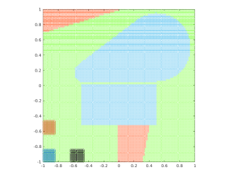
(a) Terrain and starting positions.

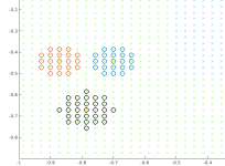
(b) Movement patterns.

Figure 3: Set-up for the numerical example. In (a), blue area is water, red area is rough terrain, and green area is normal terrain. The three different types of robots start in the three areas marked in the lower left corner: robot type 1 in the dark blue area, robot type 2 in the dark red area, and robot type 3 in the black area. In (b), the color of the (free) movement stencils are the same as the starting positions of the corresponding robot type.

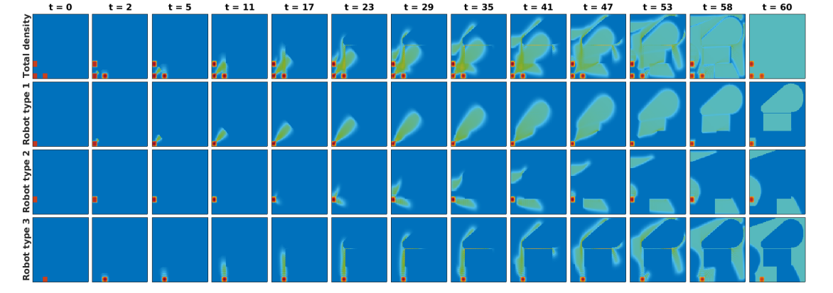
Figure 4: Time evolution of optimal total density and optimal densities of the different robots types.

V Conclusions and future directions

In this work we developed an efficient method for multispecies mean field type control problems, where each species have different dynamics. We also illustrated its use by solving a robot coordination task for a search-and-rescue-type scenario. One limitation of our method is that it becomes ill-conditioned when the intensity of noise $\epsilon$ becomes too small. One future direction is to address this issue by incorporating ideas from proximal point methods.

References

• [1] Y. Achdou, M. Bardi, and M. Cirant. Mean field games models of segregation. Mathematical Models and Methods in Applied Sciences, 27(01):75–113, 2017.
• [2] J.M. Altschuler and E. Boix-Adsera. Polynomial-time algorithms for multimarginal optimal transport problems with structure. arXiv preprint arXiv:2008.03006, 2020.
• [3] H.H. Bauschke and P.L. Combettes. Convex analysis and monotone operator theory in Hilbert spaces. Springer, Cham, 2nd edition, 2017.
• [4] J.-D. Benamou and Y. Brenier. A computational fluid mechanics solution to the Monge-Kantorovich mass transfer problem. Numerische Mathematik, 84(3):375–393, 2000.
• [5] J.-D. Benamou, G. Carlier, M. Cuturi, L. Nenna, and G. Peyré. Iterative Bregman projections for regularized transportation problems. SIAM Journal on Scientific Computing, 37(2):A1111–A1138, 2015.
• [6] J.-D. Benamou, G. Carlier, S. Di Marino, and L. Nenna. An entropy minimization approach to second-order variational mean-field games. Mathematical Models and Methods in Applied Sciences, 29(08):1553–1583, 2019.
• [7] A. Bensoussan, J. Frehse, and P. Yam. Mean field games and mean field type control theory. Springer, New York, NY, 2013.
• [8] A. Bensoussan, T. Huang, and M. Laurière. Mean field control and mean field game models with several populations. Minimax Theory and its Applications, 3(2):173–209, 2018.
• [9] B. Bonnet and H. Frankowska. Necessary optimality conditions for optimal control problems in Wasserstein spaces. Applied Mathematics & Optimization, 84:1281–1330, 2021.
• [10] P. Cardaliaguet, P.J. Graber, A. Porretta, and D. Tonon. Second order mean field games with degenerate diffusion and local coupling. Nonlinear Differential Equations and Applications NoDEA, 22(5):1287–1317, 2015.
• [11] Y. Chen, T.T. Georgiou, and M. Pavon. On the relation between optimal transport and Schrödinger bridges: A stochastic control viewpoint. Journal of Optimization Theory and Applications, 169(2):671–691, 2016.
• [12] Y. Chen, T.T. Georgiou, and M. Pavon. Optimal transport over a linear dynamical system. IEEE Transactions on Automatic Control, 62(5):2137–2152, 2017.
• [13] Y. Chen, T.T. Georgiou, and M. Pavon. Steering the distribution of agents in mean-field games system. Journal of Optimization Theory and Applications, 179(1):332–357, 2018.
• [14] Y. Chen, T.T. Georgiou, and M. Pavon. Stochastic control liasons: Richard Sinkhorn meets Gaspard Monge on a Schrödinger bridge. SIAM Review, 63(2):249–313, 2021.
• [15] M. Cirant. Multi-population mean field games systems with Neumann boundary conditions. Journal de Mathématiques Pures et Appliquées, 103(5):1294–1315, 2015.
• [16] M. Cuturi. Sinkhorn distances: Lightspeed computation of optimal transport. In Advances in Neural Information Processing Systems (NIPS), pages 2292–2300, 2013.
• [17] B. Djehiche, A. Tcheukam, and H. Tembine. Mean-field-type games in engineering. AIMS Electronics and Electrical Engineering, 1(1):18–73, 2017.
• [18] F. Elvander, I. Haasler, A. Jakobsson, and J. Karlsson. Multi-marginal optimal transport using partial information with applications in robust localization and sensor fusion. Signal Processing, 171:107474, 2020.
• [19] J. Fan, I. Haasler, J. Karlsson, and Y. Chen. On the complexity of the optimal transport problem with graph-structured cost. In Proceedings of The 25th International Conference on Artificial Intelligence and Statistics, pages 9147–9165. PMLR, 2022.
• [20] W.H. Fleming and R.W. Rishel. Deterministic and stochastic optimal control. Springer-Verlag, New York, N.Y., 1975.
• [21] H. Föllmer. Random fields and diffusion processes. In P.-L. Hennequin, editor, École d’Été de Probabilités de Saint-Flour XV–XVII, 1985–87, volume 1362 of Lecture Notes in Mathematics, pages 101–203. Springer, Berlin, Heidelberg, 1988.
• [22] W. Gangbo and A. Świkech. Optimal maps for the multidimensional Monge-Kantorovich problem. Communications on Pure and Applied Mathematics: A Journal Issued by the Courant Institute of Mathematical Sciences, 51(1):23–45, 1998.
• [23] I. Haasler, Y. Chen, and J. Karlsson. Optimal steering of ensembles with origin-destination constraints. IEEE Control Systems Letters, 5(3):881–886, 2020.
• [24] I. Haasler, A. Ringh, Y. Chen, and J. Karlsson. Estimating ensemble flows on a hidden Markov chain. In 2019 IEEE 58th Conference on Decision and Control (CDC), pages 1331–1338. IEEE, 2019.
• [25] I. Haasler, A. Ringh, Y. Chen, and J. Karlsson. Multimarginal optimal transport with a tree-structured cost and the Schrödinger bridge problem. SIAM Journal on Control and Optimization, 59(4):2428–2453, 2021.
• [26] I. Haasler, A. Ringh, Y. Chen, and J. Karlsson. Scalable computation of dynamic flow problems via multi-marginal graph-structured optimal transport. arXiv preprint arXiv:2106.14485v1, 2021.
• [27] I. Haasler, R. Singh, Q. Zhang, J. Karlsson, and Y. Chen. Multi-marginal optimal transport and probabilistic graphical models. IEEE Transactions on Information Theory, 67(7):4647–4668, 2021.
• [28] A. Hindawi, J.-B. Pomet, and L. Rifford. Mass transportation with LQ cost functions. Acta applicandae mathematicae, 113(2):215–229, 2011.
• [29] M. Huang, P.E. Caines, and R.P. Malhamé. Social optima in mean field LQG control: centralized and decentralized strategies. IEEE Transactions on Automatic Control, 57(7):1736–1751, 2012.
• [30] M. Huang, R.P. Malhamé, and P.E. Caines. Large population stochastic dynamic games: closed-loop McKean-Vlasov systems and the Nash certainty equivalence principle. Communications in Information & Systems, 6(3):221–252, 2006.
• [31] A. Lachapelle and M.-T. Wolfram. On a mean field game approach modeling congestion and aversion in pedestrian crowds. Transportation research part B: methodological, 45(10):1572–1589, 2011.
• [32] J.-M. Lasry and P.-L. Lions. Mean field games. Japanese journal of mathematics, 2(1):229–260, 2007.
• [33] C. Léonard. From the Schrödinger problem to the Monge–Kantorovich problem. Journal of Functional Analysis, 262(4):1879–1920, 2012.
• [34] C. Léonard. A survey of the Schrödinger problem and some of its connections with optimal transport. Discrete & Continuous Dynamical Systems - A, 34(4):1533–1574, 2014.
• [35] Z.-Q. Luo and P. Tseng. On the convergence of the coordinate descent method for convex differentiable minimization. Journal of Optimization Theory and Applications, 72(1):7–35, 1992.
• [36] B. Pass. Multi-marginal optimal transport: theory and applications. ESAIM: Mathematical Modelling and Numerical Analysis, 49(6):1771–1790, 2015.
• [37] G. Peyré and M. Cuturi. Computational optimal transport: With applications to data science. Foundations and Trends® in Machine Learning, 11(5-6):355–607, 2019.
• [38] A. Ringh, I. Haasler, Y. Chen, and J. Karlsson. Efficient computations of multi-species mean field games via graph-structured optimal transport. In 2021 60th IEEE Conference on Decision and Control (CDC), pages 5261–5268. IEEE, 2021.
• [39] A. Ringh, I. Haasler, Y. Chen, and J. Karlsson. Graph-structured tensor optimization for nonlinear density control and mean field games. arXiv preprint arXiv:2112.05645, 2021.
• [40] L. Rüschendorf. Optimal solutions of multivariate coupling problems. Applicationes Mathematicae, 23(3):325–338, 1995.
• [41] R. Singh, I. Haasler, Q. Zhang, J. Karlsson, and Y. Chen. Inference with aggregate data in probabilistic graphical models: An optimal transport approach. IEEE Transactions on Automatic Control, 67(9):4483–4497, 2022.
• [42] A. Terpin, N. Lanzetti, and F. Dörfler. Dynamic programming in probability spaces via optimal transport. arXiv preprint arXiv:2302.13550, 2023.
• [43] P. Tseng. Dual ascent methods for problems with strictly convex costs and linear constraints: A unified approach. SIAM Journal on Control and Optimization, 28(1):214–242, 1990.
• [44] C. Villani. Topics in optimal transportation. American Mathematical Society, Providence, RI, 2003.
• [45] M. Zorzi. Optimal transport between Gaussian stationary processes. IEEE Transactions on Automatic Control, 66(10):4939–4944, 2020.