Self-Evolution Learning for Discriminative Language Model Pretraining

Abstract

Masked language modeling, widely used in discriminative language model (e.g., BERT) pretraining, commonly adopts a random masking strategy. However, random masking does not consider the importance of the different words in the sentence meaning, where some of them are more worthy to be predicted. Therefore, various masking strategies (e.g., entity-level masking) are proposed, but most of them require expensive prior knowledge and generally train from scratch without reusing existing model weights. In this paper, we present Self-Evolution learning ($\mathbb{SE}$), a simple and effective token masking and learning method to fully and wisely exploit the knowledge from data. $\mathbb{SE}$ focuses on learning the informative yet under-explored tokens and adaptively regularizes the training by introducing a novel Token-specific Label Smoothing approach. Experiments on 10 tasks show that our $\mathbb{SE}$ brings consistent and significant improvements (+1.43$\sim$2.12 average scores) upon different PLMs. In-depth analyses demonstrate that $\mathbb{SE}$ improves linguistic knowledge learning and generalization.

1 Introduction

Masked language modeling (MLM), which commonly adopts a random masking strategy to select the mask tokens, has become the de-facto standard for discriminative pretrained language models (PLMs) Devlin et al. (2019); Liu et al. (2019); He et al. (2020); Joshi et al. (2020). However, such a random masking process is usually criticized as being sub-optimal, as it allocates an equal masking rate for all tokens. In particular, the masked tokens are sometimes too easy to guess with only local cues or shallow patterns Joshi et al. (2020), while the informative tokens that carry more critical linguistic knowledge may be neglected Church and Hanks (1990); Sadeq et al. (2022). For example, “Bush” and “Sharon” express more important meaning than “a” in the sample sentence “Bush held a talk with Sharon”. MLM with predicting the above easy-to-guess tokens, e.g., “a”, would lead to low data efficiency and sub-optimal model capability.

To address this problem, various methods have been carefully designed to improve MLM via fully leveraging the training data Sun et al. (2019); Joshi et al. (2020); Levine et al. (2020). The common goal is to inject language prior knowledge into the pretraining process Cui et al. (2022); Ding et al. (2021). Although empirically successful, there are still some limitations. First, they usually require annotation derived from off-the-shelf tools to select mask tokens, which is not only expensive but also too deterministic, and may cause error propagation from the third-party tool. For instance, Sun et al. (2019) employ external linguistic tools, e.g., Stanford CoreNLP Manning et al. (2014), to annotate the entities. Second, to ensure the effectiveness of the masking strategy, most previous works train PLM from scratch without reusing the existing models trained with vanilla MLM Sun et al. (2019); Joshi et al. (2020); Levine et al. (2020); Sadeq et al. (2022), which is wasteful and inefficient.

Thus, there raises a question: whether we can strengthen the PLM capability and data efficiency through further learning from the informative yet under-explored tokens, where such tokens are determined by the existing PLM itself. In fact, an off-the-shelf PLM already has the ability to determine the worthy and informative tokens that should be further exploited, as the representation of PLM generally can reveal good enough linguistic properties Hewitt and Manning (2019); Swayamdipta et al. (2020). For example, tokens that PLMs predict incorrect or low confidence are usually more hard-to-learn and challenging, which are essential for further training. Also, the conjecture to improve the off-the-shelf PLM is model-agnostic, green, and efficient, thus having the great potential to evolve any existing discriminative PLMs.

Motivated by this, we design a simple and effective Self-Evolution learning ($\mathbb{SE}$) mechanism to improve the pretraining of discriminative PLMs. Specifically, the $\mathbb{SE}$ contains two stages: ❶self-questioning and ❷self-evolution training. In stage 1, the PLM is forced to locate the informative but under-explored tokens from the pretraining data. After locating these hard-to-learn tokens, we then encourage the PLM to learn from them in stage 2, where we basically follow the vanilla MLM to mask these tokens and then optimize the PLM by minimizing the loss between the predictions and one-hot labels. It should be noted that due to the hard-to-learn properties, directly enforcing the PLM to fit the hard labels may lead to overfitting or overconfidence problem Miao et al. (2021). Inspired by the label smoothing (LS) Szegedy et al. (2016) that regularizes the learning by smoothing target labels with a pre-defined (static) prior distribution, we propose a novel Token-specific Label Smoothing (TLS) approach. Our TLS considers both the precise hard label and, importantly, the easily-digestible distribution that is adaptively generated by the PLM itself.

We validated our $\mathbb{SE}$ on several benchmarks including GLUE Wang et al. (2018), SuperGLUE Wang et al. (2019), SQuAD2.0 Rajpurkar et al. (2018), SWAG Zellers et al. (2018) and LAMA Petroni et al. (2019) over several PLMs: BRET Devlin et al. (2019)-Base, -Large, RoBERTa Liu et al. (2019)-Base, and -Large. Experiments demonstrate the effectiveness and universality of our approach. Extensive analyses confirm that $\mathbb{SE}$ effectively enhances the ability of PLMs on linguistic knowledge learning, model generalization and robustness.

Contributions

Our main contributions are:

• We propose $\mathbb{SE}$ to strengthen the MLM-based PLMs, where our mechanism does not require external tools and enjoys a simple recipe: continue pretraining with $\mathbb{SE}$.

• We design a novel token-specific label smoothing approach for regularization, which adopts the token-specific knowledge-intensive distributions to adaptively smooth the target labels.

• Extensive experiments show that our $\mathbb{SE}$ could significantly and robustly evolve a series of backbone PLMs, up to +2.36 average score improvement on GLUE benchmark upon RoBERTa.

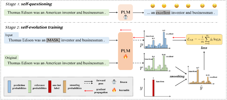
Figure 1: Overview of the proposed $\mathbb{SE}$ mechanism, which contains two stages: ❶ using an existing PLM to locate the informative yet under-explored tokens and ❷ encouraging the PLM to robustly learn from these tokens via a token-specific label smoothing approach.

2 Related Works

In recent years, we have witnessed numerous discriminative PLMs Devlin et al. (2019); Liu et al. (2019); He et al. (2020); Sun et al. (2019); Joshi et al. (2020) that achieved tremendous success in various natural language understanding (NLU) tasks. Although the discriminative PLMs vary in terms of pretraining data or model architecture, they are commonly based on MLM loss function. MLM mechanism is pioneered in BERT Devlin et al. (2019) that uses a random masking strategy to mask some tokens, and then enforces the PLM to learn to recover word information from the masked tokens. Obviously, the vanilla MLM is a linguistic-agnostic task, as the random masking procedure does not integrate linguistic knowledge explicitly, which is sub-optimal. Thus, several previous studies attempt to improve MLM by exploring a diverse of linguistically-motivated masking strategies, such as entity-level masking Sun et al. (2019), span-level masking Joshi et al. (2020), N-grams masking Levine et al. (2020), etc., to fully leverage the pretraining data.

Although achieving remarkable performance, these strategies still have some limitations. First, their implementations are relatively complex, as they usually require annotation derived from external models or tools to select tokens for masking. Even for the unsupervised PMI-masking Sadeq et al. (2022), it is still expensive to measure the pointwise mutual information for pretrain-level large-scale data, and the annotated labels are static, while our $\mathbb{SE}$ could obtain dynamic annotations via given existing PLMs. Second, in order to ensure the effectiveness of masking strategy, most previous works Sun et al. (2019); Joshi et al. (2020); Levine et al. (2020); Sadeq et al. (2022) train the language models from scratch without reusing the existing PLMs trained with vanilla MLM, which is wasteful and inefficient.

Along the same research line, in this paper, we improve the MLM-based PLMs with a novel self-evolution learning mechanism. Instead of training a PLM from scratch based on a carefully-designed and complex masking strategy, our mechanism aims to strengthen the PLM’s capability and data efficiency by further learning from the informative yet under-explored tokens, which are determined by the existing PLM itself.

3 Methodology

3.1 Preliminary

Given a sentence $S=\{t_{1},t_{2},...,t_{n}\}$ with $n$ tokens, MLM first randomly selects some percentage of the input tokens and replaces them with a special mask symbol [MASK]. Suppose that there are $m$ masked tokens and $\{k_{1},k_{2},...,k_{m}\}$ is the set of masked positions, we can denote the masked tokens as $M=\{t_{k_{1}},t_{k_{2}},...,t_{k_{m}}\}$. Let $S^{\prime}$ denote the masked sentence, we can feed $S^{\prime}$ into the model and obtain the last hidden layer representations as $H\in\mathbb{R}^{n\times d}$ ($d$ is the hidden size), and a subset of representations w.r.t masked positions as $H^{m}\in\mathbb{R}^{m\times d}$. Subsequently, the input word embedding matrix $E\in\mathbb{R}^{V\times d}$ ($V$ is the vocabulary size) is used to project the hidden representations into vocabulary space. Lastly, we can get the normalized prediction probabilities for each masked token as:

$$p_{i}=\text{softmax}(H^{m}_{i}E^{T}+b),$$ (1)

where $p_{i}\in\mathbb{R}^{V}$ and $i\in\{1,2,...,m\}$. Finally, given the one-hot labels $y_{i}$, we use the cross-entropy loss to optimize the MLM task:

$$\mathcal{L}_{MLM}=-\frac{1}{m}\sum_{i=1}^{m}y_{i}\log p_{i}$$ (2)

3.2 Self-Evolution Learning for PLMs

In this part, we introduce our $\mathbb{SE}$ mechanism in detail. At its core, $\mathbb{SE}$ is to enforce the existing PLM to further learn from the informative yet under-explored tokens, which are wisely determined by the PLM itself. Figure 1 illustrates the process of $\mathbb{SE}$ mechanism, which contains two stages: (1) self-questioning and (2) self-evolution training.

❶ Self-questioning Stage.

The goal of this stage is to select the informative yet under-explored tokens, i.e., these hard-to-learn tokens that the PLMs do not learn well during the previous pretraining. However, how to select these target tokens? Inspired by the finding of the representations of the off-the-shelf PLM on individual tokens can reveal good enough linguistic properties Hewitt and Manning (2019); Swayamdipta et al. (2020), we hereby propose to straightforwardly leverage the behavior of PLMs to wisely select target tokens in this stage. Specifically, we mainly focus on two important properties, i.e., correctness (accuracy) and confidence (the probability output that the model assigns to the prediction), as the tokens that PLMs predict incorrect or low confidence are usually more hard-to-learn and worthy for further exploring Guo et al. (2017); Park and Caragea (2022). Based on the above two properties, we introduce two simple metrics to estimate the learning value of tokens:

Correctness-based metric. In practice, we first feed the original sentence $S$ into the existing frozen PLM and enforce it to output the prediction probabilities $p_{i}$ ($i\in\{1,2,...,n\}$) for each token. Given the one-hot labels $y_{i}$ ($i\in\{1,2,...,n\}$), we calculate the cross-entropy loss (i.e., correctness) for each token position (denoted as $\{l_{1},l_{2},...,l_{n}\}$). Then, we set a loss threshold $\mathcal{T}_{l}$ and select the tokens that exceed $\mathcal{T}_{l}$ as the target tokens, i.e., $M=\{t_{i}|l_{i}>\mathcal{T}_{l}\}$ where $i\in\{1,2,...,n\}$.

Confidence-based metric. Similarly, we can measure the confidence of tokens and use it as the metric. Different from the above process, in this metric, we compute the entropy of $p_{i}$ as the confidence for each token (denoted as $\{e_{1},e_{2},...,e_{n}\}$). Intuitively, the tokens with high entropy value are hard-to-learn, as the PLM predict them with low confidence towards the gold labels. Also, an entropy threshold $\mathcal{T}_{e}$ is used to select the target tokens, i.e., $M=\{t_{i}|e_{i}>\mathcal{T}_{e}\}$.

❷ Self-evolution Training Stage.

After estimating these hard-to-learn tokens, we can then choose them for masking and encourage the PLM to learn from them. Intuitively, we can follow the vanilla MLM process to optimize the PLM by minimizing the loss between the predictions and one-hot labels, as implemented in Eq. 2. However, due to the hard-to-learn properties of these tokens, directly enforcing the PLM to fit the hard labels may lead to overfitting or overconfidence problem Miao et al. (2021); Li et al. (2022). To tackle this issue, in this stage, inspired by the label smoothing (LS) regularization approach Szegedy et al. (2016), we further propose a novel token-specific label smoothing (TLS) approach to adaptively regularize the training and improve the generalization of PLMs.

Mathematically, in LS approach, it minimizes the cross-entropy between modified label distribution $y^{\prime}_{i}$ and the model output $p_{i}$, where $y^{\prime}_{i}$ is the smoothed label distribution formulated as:

$$y^{\prime}_{i}=(1-\lambda)*y_{i}+\lambda*u_{i},$$ (3)

where $u_{i}$ is a fixed distribution that is usually a uniform distribution, and $\lambda$ is a weighting factor. Furthermore, following Yuan et al. (2020), we reformulate the loss function of LS as:

$$\mathcal{L}_{LS}=(1-\lambda)*H(y,p)+\lambda*D_{kl}(u,p),$$ (4)

where $H$ denotes the ordinary cross-entropy loss and $D_{kl}$ denotes the KL divergence loss. We can regard $D_{kl}(u,p)$ as a knowledge distillation process, where $u$ corresponds to a virtual teacher to guide the student model (i.e., the PLM). Obviously, it is sub-optimal as $u$ hardly provides enough linguistic information to guide the training of PLM.

Motivated by this, in our TLS, we design a more informative prior distribution to smooth the labels. Specifically, inspired by human learning behavior (it is often easier for humans to grasp new things described by their familiar knowledge Reder et al. (2016)), we improve the $D_{kl}$ supervision with a more easily-digestible and informative distribution that is adaptively generated by the PLM itself. In other words, $D_{kl}$ can be recast as a self-distillation process, where the virtual teacher distribution is acquired from the student model itself. In practice, for each masked position $k_{i}$, in addition to the prediction probabilities $p_{i}$ on the corrupted $S^{\prime}$, we also feed the original sentence $S$ into the current PLM and regard the corresponding probabilities as the reference probabilities $r_{i}$. Then, similar to Eq. 3, we can obtain the smoothed label $\tilde{y}_{i}$ via:

$$\tilde{y}_{i}=(1-\lambda)*y_{i}+\lambda*r_{i}$$ (5)

Lastly, we use the cross-entropy as the loss function in the $\mathbb{SE}$ training stage, as follows:

$$\mathcal{L}_{SE}=-\frac{1}{m}\sum_{i=1}^{m}\tilde{y}_{i}\log p_{i}$$ (6)

	CoLA	MRPC	RTE	BoolQ	CB	WiC	COPA	Score
Method	Mcc.	Acc.	Acc.	Acc.	Acc.	Acc.	Acc.	Avg.	$\Delta$ ($\uparrow$)
Performance of Different Masking Strategies
BERT$\rm{}_{\texttt{base}}$	62.33	88.97	76.89	75.05	85.71	66.77	63.00	74.10	–
-w/ Entity-level masking	60.06	88.73	76.53	74.77	87.50	66.61	65.00	74.17	+0.07
-w/ Span-level masking	61.41	88.48	78.34	74.28	87.50	67.40	65.00	74.63	+0.53
-w/ PMI-based masking	61.09	88.24	76.90	74.25	87.50	66.61	65.00	74.23	+0.13
-w/ Self-questioning	63.78	87.99	78.34	74.13	85.71	67.87	66.00	74.83	+0.73
BERT-SE$\rm{}_{\texttt{base}}$	63.63	89.50	77.98	74.37	89.29	67.40	66.00	75.45	+1.35
Performance upon More Discriminative PLMs
BERT$\rm{}_{\texttt{large}}$	63.00	87.25	83.80	78.40	91.07	67.24	72.00	77.54	–
BERT-SE$\rm{}_{\texttt{large}}$	65.66	88.23	85.20	80.18	92.86	68.34	78.00	79.78	+2.24
RoBERTa$\rm{}_{\texttt{base}}$	62.00	90.20	83.12	78.72	83.93	69.12	70.00	76.72	–
RoBERTa-SE$\rm{}_{\texttt{base}}$	62.11	89.71	84.12	79.39	92.86	71.40	74.00	79.08	+2.36
RoBERTa$\rm{}_{\texttt{large}}$	64.73	90.69	88.44	84.37	91.07	69.90	78.00	81.03	–
RoBERTa-SE$\rm{}_{\texttt{large}}$	67.80	91.91	90.25	84.56	96.40	70.53	80.00	83.06	+2.03

Table 1: Comparison between our $\mathbb{SE}$ and the vanilla method applied to all PLMs on the combination of GLUE and SuperGLUE benchmarks. Average scores on all tasks are underlined. The best results are given in bold. “$\Delta$” denotes the improvement of $\mathbb{SE}$ methods compared to the baseline PLMs.

4 Experiments

4.1 Tasks and Datasets

We follow many previous studies Zhong et al. (2022a, c, 2023a, 2023b) and conduct extensive experiments on various NLU tasks, including a diversity of tasks from GLUE Wang et al. (2018) and SuperGLUE Wang et al. (2019) benchmarks, i.e., linguistic acceptability (CoLA), natural language inference (RTE, CB), paraphrase (MRPC), question answering (BoolQ), word sense disambiguation (WiC) and causal reasoning (COPA). Additionally, we also evaluate on three knowledge-intense tasks, which require the ability of commonsense knowledge reasoning, i.e., SQuAD2.0 Rajpurkar et al. (2018), SWAG Zellers et al. (2018) and LAMA Petroni et al. (2019). In practice, we report the performance with Accuracy (“Acc.”) metric for most tasks, except the Matthew correlation (“Mcc.”) for CoLA, the F1 and Exact Match (“EM”) scores for SQuAD2.0, and the Mean Reciprocal Rank (“MRR”) scores for LAMA. We report the averaged results over 10 random seeds to avoid stochasticity. The details of all tasks and datasets are provided in Appendix A.1.

4.2 Implementation Details

Pre-training.

We employ the representative BRET Devlin et al. (2019)-Base, -Large, RoBERTa Liu et al. (2019)-Base, and -Large as the backbone discriminative PLMs, and implement our methods in a continued pretraining manner. For pretraining settings, we follow the original papers Devlin et al. (2019); Liu et al. (2019) and use the same pretraining corpus and (most of) hyper-parameters (e.g., batch size and the maximum length of the input sentence), respectively.

Especially, as suggested by Liu et al. (2019), we do not use the next sentence prediction (NSP) objective during BERT pretraining. For our methods, we continue pretraining the backbone PLMs with 2 epochs. Additionally, for reference, we train the PLMs with the vanilla MLM for the same steps and refer to them as the baselines.

Fine-tuning.

The learning rate is selected in {1e-5, 2e-5, 3e-5, 5e-5}, while the batch size is in {12, 16, 32} depending on tasks. The maximum length of the input sentence is 384 for SQuAD2.0 and 256/512 for other tasks. We use AdamW Loshchilov and Hutter (2018) as the optimizer, and set the $\beta_{2}$ and weight decay as 0.98 and 0.01, respectively. All experiments are conducted on NVIDIA A100 GPUs. The detailed hyper-parameters are provided in Appendix A.2.

Compared Methods.

For references, we compare our $\mathbb{SE}$ method with other cutting-edge counterparts. Specifically, taking the BERT$\rm{}_{\texttt{base}}$ as the baseline, we use the following masking strategies to further improve its performance:

• Entity-level masking: following Sun et al. (2019), we mask the named entities in the sentence and enforce the model to predict them.

• Span-level masking: as done in Joshi et al. (2020), we randomly select spans from the sentence based on a geometric distribution and mask the selected span.

• PMI-based masking: similar to Sadeq et al. (2022), we use PMI to identify a set of contiguous (informative) N-grams and mask them.

• Self-questioning masking: We adopt our stage 1 to select the hard-to-learn tokens and directly follow the vanilla MLM to mask them and predict the one-hot labels.

Notably, for a fair comparison, we implement all these methods in a continual pretraining manner, same to the settings of our $\mathbb{SE}$.

Method	SQuAD2.0		SWAG	Avg.
	EM	F1	Acc.
BERT$\rm{}_{\texttt{base}}$	72.18	75.07	77.53	74.93
BERT-SE$\rm{}_{\texttt{base}}$	72.89	75.64	77.91	75.48
BERT$\rm{}_{\texttt{large}}$	81.35	84.38	83.40	83.04
BERT-SE$\rm{}_{\texttt{large}}$	81.94	85.00	83.61	83.52
RoBERTa$\rm{}_{\texttt{base}}$	78.79	81.92	79.69	80.13
RoBERTa-SE$\rm{}_{\texttt{base}}$	79.41	82.55	79.88	80.61
RoBERTa$\rm{}_{\texttt{large}}$	84.70	87.65	84.34	85.56
RoBERTa-SE$\rm{}_{\texttt{large}}$	85.03	87.93	84.54	85.83

Table 2: Performance on SQuAD2.0 Rajpurkar et al. (2018) and SWAG Zellers et al. (2018) dev sets.

Method	Google-RE (LAMA)			Avg.
	date-birth	place-birth	place-death
RoBERTa$\rm{}_{\texttt{base}}$	5.51	11.52	2.68	6.57
RoBERTa-SE$\rm{}_{\texttt{base}}$	6.35	15.16	9.61	10.37

Table 3: Performance of our $\mathbb{SE}$ on LAMA Petroni et al. (2019) to probe the factual knowledge.

Method	BERT$\rm{}_{\texttt{base}}$	BERT$\rm{}_{\texttt{large}}$	RoBERTa$\rm{}_{\texttt{base}}$	RoBERTa$\rm{}_{\texttt{large}}$	Avg.
Baseline	74.10	77.54	76.73	81.03	77.35
Selecting metrics in self-questioning stage
-w/ randomly selecting	73.85 (-0.25)	78.28 (+0.74)	77.09 (+0.36)	81.64 (+0.61)	77.72 (+0.37)
-w/ Correctness-based	75.45 (+1.35)	79.78 (+2.24)	79.08 (+2.35)	83.06 (+2.03)	79.34 (+1.99)
-w/ Confidence-based	75.77 (+1.67)	78.88 (+1.34)	77.86 (+1.13)	82.46 (+1.43)	78.74 (+1.39)

Table 4: Ablation study of different metrics used to select the hard-to-learn tokens in $\mathbb{SE}$, evaluated on the combination of GLUE and SuperGLUE benchmarks. For simplicity, we show the overall score here. The full results and analyses about the superiority of the correctness-based metric can be found in Appendix (Table 11&10).

4.3 Main Results

$\mathbb{SE}$ surpasses the previous carefully-designed masking strategies.

Results on GLUE and SuperGLUE benchmarks are shown in Table 1. Compared with the baseline BERT$\rm{}_{\texttt{base}}$, all masking strategies bring the average performance gains, proving the necessity of improving MLM. Among all these methods, our proposed self-questioning masking achieves the relatively better performance on many tasks, confirming the effectiveness of using the PLMs themselves to select the hard-to-learn tokens. More encouragingly, with the help of self-evolution training, our final BERT-SE$\rm{}_{\texttt{base}}$ can achieve further performance improvements. These results can prove the superiority of our $\mathbb{SE}$.

$\mathbb{SE}$ brings consistent and significant performance improvements among all PLMs.

In addition to the results upon BERT$\rm{}_{\texttt{base}}$, we also apply our method on more discriminative PLMs and report the results in Table 1. Compared with the baselines, $\mathbb{SE}$ brings consistent and significant performance improvements across all BERT/RoBERTa model sizes. Specifically, for Base and Large RoBERTa models, $\mathbb{SE}$ brings 2.36% and 2.03% relative gains in overall score respectively. Also, the gain for BERT is up to 2.24%. These results prove the effectiveness and universality of our $\mathbb{SE}$.

$\mathbb{SE}$ enhances the ability of knowledge learning.

For the knowledge-intense tasks, i.e., SQuAD2.0 and SWAG, we report the results in Table 2. With the help of $\mathbb{SE}$, all PLMs consistently achieve better performance. Specifically, the performance improvements on SQuAD2.0 in terms of EM and F1 are up to 0.71% and 0.64%, respectively. Besides QA tasks that require to be fine-tuned, we conduct experiments on a widely-used factual knowledge probing task, i.e., LAMA Petroni et al. (2019), to verify whether $\mathbb{SE}$ improves the ability of PLMs on commonsense knowledge. We report the results in Table 3. Based on the powerful RoBERTa, $\mathbb{SE}$ still brings significant improvements, i.e. +3.8 average score, to the knowledge-learning ability of PLMs.

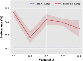
Figure 2: Parameter analysis of $\lambda$ on BERT-SE$\rm{}_{\texttt{large}}$.

4.4 Ablation Study

We evaluate the impact of each component of our $\mathbb{SE}$, including i) token-selecting metrics, ii) token-specific label smoothing approach, iii) coefficient $\lambda$, and iv) more $\mathbb{SE}$ iterations.

Impact of Token Selecting Metrics.

As mentioned in §3.2, we introduce several metrics to select the hard-to-learn tokens in the self-questioning stage. Here, we conduct experiments to analyze the impact of different metrics. Specifically, for reference, we compare the “Correctness-based” and “Confidence-based” metrics with a simple alternative, i.e., “randomly selecting”. Results in Table 4.2 show that 1) although the “randomly selecting” performs worst, it still outperforms the continually trained baseline, showing the effectiveness of the self-evolution training. 2) both our proposed metrics “Correctness-based” and “Confidence-based” achieve significantly better performance, confirming our claim that learning on informative yet under-explored tokens can strengthen the capability of PLMs and data efficiency. Notably, the correctness-based metric outperforms the confidence-based metric in most cases, thus leaving as our default setting in $\mathbb{SE}$.

Method	GLUE/SGLUE	SQuAD/SWAG
	Avg. ($\Delta\uparrow$)	Avg. ($\Delta\uparrow$)
RoBERTa$\rm{}_{\texttt{base}}$	76.73	80.13
RoBERTa-SE$\rm{}_{\texttt{base}}$
-w/ vanilla LS	78.37 (+1.64)	80.37 (+0.24)
-w/ TLS (Ours)	79.08 (+2.35)	80.61 (+0.48)

Table 5: Ablation study of our TLS approach. “-w/ vanilla LS” and “-w/ TLS (Ours)” refer to using the vanilla and our proposed token-specific label smoothing approaches in $\mathbb{SE}$ mechanism, respectively. Full results are shown in Appendix (Table A.5).

Impact of Token-specific Label Smoothing.

A key technology in our $\mathbb{SE}$ is the TLS, which uses the token-specific smoothed label to adaptively guide training. To verify its effectiveness, we conduct experiments and present the results in Table 4.4. We show that 1) the vanilla label smoothing approach equipped $\mathbb{SE}$ could easily outperform the continuously trained backbone, showing the superiority of our $\mathbb{SE}$ framework, and importantly, 2) our TLS could further improve the results by a large margin against vanilla LS equipped $\mathbb{SE}$, e.g. averaging +0.71, indicating the effectiveness of TLS.

Impact of Coefficient $\lambda$.

The factor $\lambda$ in Eq. 5, which is used to control the ratio of label smoothing, is an important hyper-parameters. In this study, we analyze its influence by evaluating the performance with different $\lambda$ spanning {0.1, 0.3, 0.5, 0.7, 0.9} on several GLUE tasks. Figure 2 illustrates the average results. Compared with the baseline, our $\mathbb{SE}$ consistently brings improvements across all ratios of $\lambda$, basically indicating that the performance of $\mathbb{SE}$ is not sensitive to $\lambda$. More specifically, the case of $\lambda=0.1$ performs best, and we thereby use this setting in our experiments.

GLUE	$N=1$	$N=2$	$N=3$
CoLA	63.63	63.59	63.60
MRPC	89.50	88.23	88.97
RTE	77.98	79.42	78.70
Avg. ($\Delta\uparrow$)	+0.97	+1.02	+1.03

Table 6: Performance for different iterations $N$ on BERT-SE${}_{\texttt{base}}$. “Avg. ($\Delta\uparrow$)” indicates the relative improvement against the vanilla BERT${}_{\texttt{base}}$.

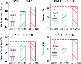
Figure 3: Analysis of task generalization. The model is fine-tuned on the QNLI task and transferred to four different tasks. We can see that $\mathbb{SE}$ consistently brings better generalization compared with its counterparts.

Figure 4: The 3D loss surface comparison between baseline, $\mathbb{SE}$ (“-w/ vanilla LS”) and $\mathbb{SE}$ (“-w/ TLS”) methods applied to RoBERTa$\rm{}_{\texttt{base}}$. Note that the PLMs are fine-tuned on the CoLA task.

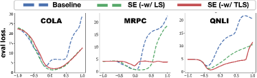
Figure 5: 1D visualization of loss landscapes of RoBERTa$\rm{}_{\texttt{base}}$ models fine-tuned on different tasks.

Impact of More $\mathbb{SE}$ Iterations.

Researchers may doubt whether $\mathbb{SE}$ can be further augmented by performing the self-questioning and token-specific label smoothing with already evolved PLMs that own better representations. That is, whether more iterations (denoted as “$N$”) further enhance $\mathbb{SE}$? To answer this question, we continuously train the PLMs with more $\mathbb{SE}$ iterations and report the performance of several GLUE tasks in Table 6. As seen, increasing the iterations improves the performance but the gain margin is insignificant. Given that increasing $N$ costs more, we suggest using $\mathbb{SE}$ for only one iteration to achieve a better trade-off between costs and performance.

5 Discussion

To better understand $\mathbb{SE}$, we conduct extensive analyses to discuss whether it gains better generalization/ robustness and knowledge-learning ability.

5.1 Does $\mathbb{SE}$ Bring Better Generalization?

We examine from two perspectives: i) measuring the cross-task zero-shot performance, and ii) visualizing the loss landscapes of PLMs.

Task Generalization.

The performance of out-of-domain (OOD) data is widely used to verify the model generalization Wang et al. (2022); Ding et al. (2022). Thus, we follow Xu et al. (2021); Zhong et al. (2022b) and evaluate the performance of PLMs on several OOD data. In practice, we first fine-tune RoBERTa$\rm{}_{\texttt{base}}$ models trained with different methods (including “Baseline”, “$\mathbb{SE}$ (-w/ LS)”, and “$\mathbb{SE}$ (-w/ TLS)”) on the QNLI task, and then inference on other tasks, i.e., CoLA, MRPC, STS-B, and RTE. The results are illustrated in Figure 3. We observe that “$\mathbb{SE}$ (-w/ TLS)” consistently outperforms the other counterparts. To be more specific, compared with baseline, our $\mathbb{SE}$ brings a +2.90 average improvement score on these tasks, indicating that our $\mathbb{SE}$ boosts the performance of PLMs on OOD data.

Visualization of Landscape.

To have a close look, we visualize the loss landscapes of different RoBERTa$\rm{}_{\texttt{base}}$ models fine-tuned on the CoLA task. In practice, we first show the 3D loss surface results in Figure 4 following the “filter normalized” setting in Li et al. (2018); Zan et al. (2022). As seen, $\mathbb{SE}$-equipped PLMs show flatter smoother surfaces compared with the vanilla. To closely compare the differences of “$\mathbb{SE}$ (-w/ LS)” and “$\mathbb{SE}$ (-w/ TLS)” in the loss landscape, we follow He et al. (2021) to plot the 1D loss curve on more tasks in Figure 5. We find that through detailed 1D visualization, our optimal setting “$\mathbb{SE}$ (-w/ TLS)” shows a flatter and optimal property. These results prove that $\mathbb{SE}$ can smooth the loss landscape and improve the generalization of PLMs effectively.

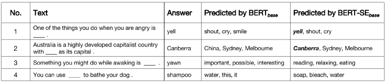
Figure 6: Cloze test comparison between BERT$\rm{}_{\texttt{base}}$ and BERT-SE$\rm{}_{\texttt{base}}$. The correct predictions are in bold.

5.2 Cloze Test

To verify whether $\mathbb{SE}$ enforces the PLMs to learn from the informative tokens, we follow Sun et al. (2019) and apply the Cloze test Taylor (1953) to evaluate the knowledge learning ability of PLMs. For each test sample, we first remove the informative token and then enforce the PLMs to infer what it is. Some cases are shown in Figure 6.

In case 1 and case 2, both BERT$\rm{}_{\texttt{base}}$ and BERT-SE$\rm{}_{\texttt{base}}$ can successfully predict the type of masked tokens according to the contexts. However, with the help of the $\mathbb{SE}$ mechanism, BERT-SE$\rm{}_{\texttt{base}}$ performs more correctly on filling in the slot. Dramatically, in case 3, the baseline BERT$\rm{}_{\texttt{base}}$ makes unreasonable predictions. One possible reason is that the baseline PLM only learns the shallow pattern and fails to understand the meaning of the context. Additionally, due to the unsatisfactory ability of the baseline PLM on commonsense reasoning, the baseline PLM also predicts strangely in case 4. Different from the baseline, while BERT-SE$\rm{}_{\texttt{base}}$ does not predict the completely correct tokens in case 3 and case 4, it can capture deep patterns and make more reasonable predictions. In general, these cases prove that $\mathbb{SE}$ indeed improves the knowledge-learning ability of PLMs.

☞ More analyses in Appendix

In addition to the above discussions, we conduct more related analyses and show them in Appendix, e.g., parameter analyses on $\mathcal{T}_{l}$ and $\mathcal{T}_{e}$ (Appendix A.4), robustness analysis based on the empirical results on AdvGLUE Wang et al. (2021) (Appendix A.3), and non-complementarity analysis between token-selecting metrics (Appendix A.5). Please refer to Appendix for more details.

6 Conclusion

In this paper, we propose a simple and effective self-evolution ($\mathbb{SE}$) learning mechanism to improve the existing discriminative PLMs by fully exploiting the knowledge from data. $\mathbb{SE}$ follows two stages, i.e., self-questioning and self-evolution training, and can be used to evolve any MLM-based PLMs with a simple recipe: continue pretraining with $\mathbb{SE}$. We empirically demonstrated the effectiveness and universality of the $\mathbb{SE}$ on a series of widely-used benchmarks. Further analyses show our approach improves the generalization, robustness, and knowledge-learning ability. We hope our work could facilitate more research on how to improve existing trained models after all the previous PLM weights are expensive and knowledgeable.

Limitations

Our work has several potential limitations. First, given the limited computational budget, we only validate our self-evolution learning on the Large and Base sizes. It will make our work more convincing if scaling the experiments up to the larger model size and training corpus. On the other hand, besides the improved commonsense knowledge learning ability, we believe that there are still other abilities, e.g., mathematical word problems, of PLMs that can be improved by our method, which are not fully explored in this work.

Ethics and Reproducibility Statements

Ethics

We take ethical considerations very seriously, and strictly adhere to the ACL Ethics Policy. This paper focuses on higher data and model efficiency for discriminative pretrained language models, but not capturing the privacy knowledge. Both the pretraining datasets and models used in this paper are publicly available and have been widely adopted by researchers. Therefore, we believe that this research will not pose ethical issues.

Reproducibility

We will publicly release our code in https://github.com/WHU-ZQH/SE4PLMs to help reproduce the experimental results of this paper.

Acknowledgements

We are grateful to the anonymous reviewers and the area chair for their insightful comments and suggestions. This work was supported in part by the National Natural Science Foundation of China under Grants 62225113 and 62076186, and in part by the Science and Technology Major Project of Hubei Province (Next-Generation AI Technologies) under Grant 2019AEA170. The numerical calculations in this paper have been done on the supercomputing system in the Supercomputing Center of Wuhan University.

Appendix A Appendix

Task		#Train	#Dev	#Class	LR	BSZ	Epochs/Steps
GLUE	CoLA	8.5K	1,042	2	2e-5	32	2668 steps
	MRPC	3.7K	409	2	1e-5	32	1148 steps
	RTE	2.5K	278	2	1e-5	16	2036 steps
SuperGLUE	BoolQ	9.4K	3,270	2	1e-5	16	10 epochs
	CB	250	57	2	2e-5	16	20 epochs
	WiC	6K	638	2	2e-5	16	10 epochs
	COPA	400	100	2	2e-5	16	10 epochs
Commonsense QA	SQuAD2.0	130K	11,873	-	3e-5	12	2 epochs
	SWAG	73K	20K	-	5e-5	16	3 epochs
LAMA	Google-RE	60K		-	N/A

Table 7: Data statistics and fine-tuning hyper-parameters of all used tasks in this paper. “Class” refers to the label class, “LR” means the learning rate and “BSA” denotes the batch size. Note that the LAMA benchmark is wrapped into a cloze test to probe the PLM without fine-tuning.

Method	BERT$\rm{}_{\texttt{base}}$						RoBERTa$\rm{}_{\texttt{base}}$
	RTE	SST-2	QNLI	MNLI	QQP	Avg.	RTE	SST-2	QNLI	MNLI	QQP	Avg.
Baseline	32.8	29.7	40.5	22.8	38.5	32.9	47.1	41.9	36.2	21.0	30.9	35.4
-w/ SE	33.3	28.4	42.6	23.5	42.3	34.0	45.7	37.8	32.4	23.5	38.5	35.6
Method	BERT$\rm{}_{\texttt{large}}$						RoBERTa$\rm{}_{\texttt{large}}$
	RTE	SST-2	QNLI	MNLI	QQP	Avg.	RTE	SST-2	QNLI	MNLI	QQP	Avg.
Baseline	45.6	35.8	41.4	25.3	45.4	38.7	64.1	43.9	61.5	33.9	44.9	49.7
-w/ SE	53.1	35.1	45.3	24.7	50.0	41.6	67.9	48.6	58.1	34.6	55.1	52.9

Table 8: Comparison between $\mathbb{SE}$ and vanilla method applied to all PLMs on AdvGLUE Wang et al. (2021) benchmark. Average scores on all tasks are underlined. The best results are given in bold.

A.1 Details of Tasks and Datasets

Here, we introduce the descriptions of all downstream tasks and datasets in detail. Firstly, we present the statistics of all datasets in Table 7. Then, each task is described as:

CoLA Corpus of Linguistic Acceptability Warstadt et al. (2019) is a binary single-sentence classification task to determine whether a given sentence is linguistically “acceptable”.

MRPC Microsoft Research Paraphrase Corpus Dolan and Brockett (2005) is a task to predict whether two sentences are semantically equivalent.

RTE Recognizing Textual Entailment Giampiccolo et al. (2007), given a premise and a hypothesis, is a task to predict whether the premise entails the hypothesis.

QNLI Question Natural Language Inference is a binary classification task constructed from SQuAD Rajpurkar et al. (2016), which aims to predict whether a context sentence contains the answer to a question sentence.

CB CommitmentBank De Marneffe et al. (2019) can be framed as three-class textual entailment on a corpus of 1,200 naturally occurring discourses.

BoolQ Boolean Question Clark et al. (2019) is a question answering task where each sample consists of a short passage and a yes/no question about the passage.

WiC Word-in-Context Pilehvar and Camacho-Collados (2019) is a word sense disambiguation task that aims to predict whether the word is used with the same sense in sentence pairs.

COPA Choice of Plausible AlternativesRoemmele et al. (2011) is a causal reasoning task in which a system is given a premise sentence and must determine either the cause or effect of the premise from two possible choices.

SQuAD2.0 The latest version of the Stanford Question Answering Dataset Rajpurkar et al. (2018) is one of the most widely-used reading comprehension benchmarks that require the systems to acquire knowledge reasoning ability.

SWAG Situations With Adversarial Generations Zellers et al. (2018) is a task of grounded commonsense inference, which unified natural language inference and commonsense reasoning. It is also widely used to evaluate the ability of PLMs on commonsense knowledge reasoning.

Google-RE The Google-RE corpus contains  60K facts manually extracted from Wikipedia. The LAMA Petroni et al. (2019) benchmark manually defines a template for each considered relation, e.g., “[S] was born in [O]” for “place of birth”. Each fact in the Google-RE dataset is, by design, manually aligned to a short piece of Wikipedia text supporting it. There is no training process and during inference, we query the PLMs using a standard cloze template for each relation. It is widely used to probe the model’s world knowledge, especially factual knowledge.

A.2 Hyper-parameters of Fine-tuning

For fine-tuning, we use the BERT and RoBERTa models as the backbone PLMs and conduct experiments using the open-source toolkit fairseq and transformers. Notably, we apply the same hyper-parameters to all PLMs for simplicity. The training epochs/steps, batch size, and learning rate for each downstream task are listed in Table 7.

A.3 Does $\mathbb{SE}$ Improve the Robustness?

Here, we conduct experiments to verify whether $\mathbb{SE}$ improves the robustness of PLMs. In practice, following Jiang et al. (2022), we use the Adversarial GLUE (AdvGLUE) Wang et al. (2021), which is a robustness benchmark that was created by applying 14 textual adversarial attack methods to GLUE tasks, to measure the robustness in this study. Table 8 lists the results on all PLMs. With the help of our $\mathbb{SE}$ method, the PLMs achieve consistent improvements on the AdvGLUE benchmark. These results prove that our $\mathbb{SE}$ method is beneficial to the robustness of PLMs.

Method	GLUE/SGLUE	SQuAD2.0/SWAG
	Avg. ($\Delta$)	Avg. ($\Delta$)
BERT$\rm{}_{\texttt{base}}$	74.10	74.93
BERT-SE$\rm{}_{\texttt{base}}$
$\mathcal{T}_{l}=0.05$	74.63 (+0.53)	75.44 (+0.51)
$\mathcal{T}_{l}=0.1$	75.45 (+1.35)	75.48 (+0.55)
$\mathcal{T}_{l}=0.5$	73.93 (-0.17)	75.22 (+0.29)
$\mathcal{T}_{l}=1$	74.02 (-0.08)	75.37 (+0.44)

Table 9: Parameter analysis on the threshold $\mathcal{T}_{l}$ used in self-questioning stage. The “Correctness-based” metric is used in this study. Full results are in Table A.5.

A.4 Parameter Analyses on $\mathcal{T}_{l}$ and $\mathcal{T}_{e}$

As stated in §3.2, we respectively set a threshold $\mathcal{T}_{l}$ and $\mathcal{T}_{e}$ for the Correctness-based and Confidence-based metrics to select the hard-to-learn tokens. Here, we analyze the influence of different $\mathcal{T}$ in detail. In practice, taking the $\mathcal{T}_{l}$ as an example, we train the BERT$\rm{}_{\texttt{base}}$ with different $\mathcal{T}_{l}$ (in {0.05,0.1,0.5,1}) and evaluate the performance on a combination of GLUE, SuperGLUE (SGLUE for short), SQuAD2.0 and SWAG benchmarks. Table A.3 lists the average scores of these benchmarks.

Specifically, when the $\mathcal{T}_{l}$ (i.e., 0.05) is too small, there may be too many easy-to-learn tokens selected by the metric, which could make the PLM pay less attention to the target hard-to-learn tokens and thus slightly affect the efficacy of $\mathbb{SE}$ mechanism. On the other hand, increasing the $\mathcal{T}_{l}$ makes it hard to learn the few amounts but greatly challenging tokens, thus slightly harming the performance on GLUE/SGLUE. Among them, $\mathcal{T}_{l}=0.1$ achieves the best, thus leaving as the default setting for correctness-based metric.

JS($P_{1}||P_{2}$)	KL($P_{2}||P_{1}$)	KL($P_{1}||P_{2}$)
0.1681	0.3875	0.7506

Table 10: Distribution difference between vocabulary distributions selected by Correctness-based “$P_{1}$” and Confidence-based “$P_{2}$” metrics. BERT-SE$\rm{}_{\texttt{large}}$ is used.

A.5 Analysis of non-complementarity between token-selecting metrics.

As aforementioned in the ablation study, costly combining both correctness- and confidence-based metrics to select the tokens in the self-questioning stage does not show complementarity, having not outperformed the default one (correctness-based). To explain their non-complementarity, we quantitatively analyze the difference in their vocabulary distributions in Table 10.

Specifically, let $P_{1}$ and $P_{2}$ denote the token frequency distributions of “Correctness-based” and “Confidence-based” metrics, respectively. We first use the Jensen-Shannon (JS) divergence Lin (1991) to measure the overall difference between $P_{1}$ and $P_{2}$. It can be found that the JS($P_{1}||P_{2}$) is only 0.1681, indicating that both distributions are overall similar. Furthermore, to fine-grained analyze the impact of both distributions on each other, we compute the KL divergence Kullback and Leibler (1951) for $P_{1}\xrightarrow{}P_{2}$ (i.e., KL($P_{2}||P_{1}$)) and $P_{2}\xrightarrow{}P_{1}$ (i.e., KL($P_{1}||P_{2}$)), respectively. Clearly, estimating $P_{2}$ based on $P_{1}$ is much easier than the opposite direction, i.e., KL($P_{2}||P_{1}$) $<$ KL($P_{1}||P_{2}$), indicating that tokens selected by the correctness-based metric contain most of those selected by confidence-based metric. These statistics nicely explain the empirical superiority of the correctness-based metric in Table 4.2.

	CoLA	MRPC	RTE	BoolQ	CB	WiC	COPA	Score
Method	Mcc.	Acc.	Acc.	Acc.	Acc.	Acc.	Acc.	Avg.	$\Delta$
Baseline PLMs
BERT$\rm{}_{\texttt{base}}$	62.33	88.97	76.89	75.05	85.71	66.77	63.00	74.10	–
BERT$\rm{}_{\texttt{large}}$	63.00	87.25	83.80	78.40	91.07	67.24	72.00	77.54	–
RoBERTa$\rm{}_{\texttt{base}}$	62.00	90.20	83.12	78.72	83.93	69.12	70.00	76.73	–
RoBERTa$\rm{}_{\texttt{large}}$	64.73	90.69	88.44	84.37	91.07	69.90	78.00	81.03	–
“Randomly selecting”
BERT-SE$\rm{}_{\texttt{base}}$	63.23	87.01	76.17	74.83	85.70	68.00	62.00	73.85	-0.25
BERT-SE$\rm{}_{\texttt{large}}$	65.28	87.74	84.12	80.10	92.90	68.8	69.00	78.28	+0.74
RoBERTa-SE$\rm{}_{\texttt{base}}$	63.78	88.73	81.59	78.83	89.29	69.43	68.00	77.09	+0.36
RoBERTa-SE$\rm{}_{\texttt{large}}$	63.42	90.20	89.89	84.13	92.86	71.00	80.00	81.64	+0.61
“Correctness-based” metric
BERT-SE$\rm{}_{\texttt{base}}$	63.63	89.50	77.98	74.37	89.29	67.40	66.00	75.45	+1.35
BERT-SE$\rm{}_{\texttt{large}}$	65.66	88.23	85.20	80.18	92.86	68.34	78.00	79.78	+2.24
RoBERTa-SE$\rm{}_{\texttt{base}}$	62.11	89.71	84.12	79.39	92.86	71.40	74.00	79.08	+2.35
RoBERTa-SE$\rm{}_{\texttt{large}}$	67.80	91.91	90.25	84.56	96.40	70.53	80.00	83.06	+2.03
“Confidence-based” metric
BERT-SE$\rm{}_{\texttt{base}}$	63.17	89.22	80.51	73.98	89.29	67.24	67.00	75.77	+1.67
BERT-SE$\rm{}_{\texttt{large}}$	64.07	88.48	84.84	79.30	92.86	69.59	73.00	78.88	+1.34
RoBERTa-SE$\rm{}_{\texttt{base}}$	64.06	89.71	83.03	78.10	85.71	69.44	75.00	77.86	+1.13
RoBERTa-SE$\rm{}_{\texttt{large}}$	64.17	89.71	90.61	84.13	96.40	70.22	82.00	82.46	+1.43

Table 11: Full comparison results (corresponding to the average results in Table 4.2) between different metrics used to select the hard-to-learn tokens on the combination of GLUE and SuperGLUE benchmarks. “$\Delta$” denotes the improvement of $\mathbb{SE}$ methods compared to the baseline PLMs. Average scores on all tasks are underlined.

	CoLA	MRPC	RTE	BoolQ	CB	WiC	COPA	SQuAD2.0		SWAG
Method	Mcc.	Acc.	Acc.	Acc.	Acc.	Acc.	Acc.	EM	F1	Acc.
RoBERTa$\rm{}_{\texttt{base}}$	62.00	90.20	83.12	78.72	83.93	69.12	70.00	78.79	81.92	79.69
RoBERTa-SE$\rm{}_{\texttt{base}}$
-w/ vanilla LS	63.18	89.71	83.39	78.29	89.29	69.75	75.00	79.01	82.12	79.97
-w/ TLS (Ours)	62.11	89.71	84.12	79.39	92.86	71.40	74.00	79.41	82.55	79.88
BERT$\rm{}_{\texttt{base}}$	62.33	88.97	76.89	75.05	85.71	66.77	63.00	72.85	75.63	77.83
BERT-SE$\rm{}_{\texttt{base}}$
$\mathcal{T}_{l}=0.05$	63.30	87.50	77.26	73.91	85.71	67.71	67.00	72.85	75.63	77.83
$\mathcal{T}_{l}=0.1$	63.63	89.50	77.98	74.37	89.29	67.40	66.00	72.89	75.64	77.91
$\mathcal{T}_{l}=0.5$	61.31	88.24	77.26	73.88	85.71	67.08	64.00	72.46	75.36	77.84
$\mathcal{T}_{l}=1$	62.06	88.24	77.26	73.82	82.14	68.65	66.00	72.62	75.56	77.93

Table 12: Full comparison results (corresponding to the average results in Table 4.4 and A.3, respectively) on the combination of GLUE, SuperGLUE, SQuAD2.0 and SWAG benchmarks. Best results are given in bold.

References

- Church and Hanks (1990) Kenneth Church and Patrick Hanks. 1990. Word association norms, mutual information, and lexicography. Computational linguistics.
- Clark et al. (2019) Christopher Clark, Kenton Lee, Ming-Wei Chang, Tom Kwiatkowski, Michael Collins, and Kristina Toutanova. 2019. Boolq: Exploring the surprising difficulty of natural yes/no questions. In NAACL.
- Cui et al. (2022) Yiming Cui, Wanxiang Che, Shijin Wang, and Ting Liu. 2022. Lert: A linguistically-motivated pre-trained language model. arXiv.
- De Marneffe et al. (2019) Marie-Catherine De Marneffe, Mandy Simons, and Judith Tonhauser. 2019. The commitmentbank: Investigating projection in naturally occurring discourse. In proceedings of Sinn und Bedeutung.
- Devlin et al. (2019) Jacob Devlin, Ming-Wei Chang, Kenton Lee, and Kristina Toutanova. 2019. Bert: Pre-training of deep bidirectional transformers for language understanding. In NAACL.
- Ding et al. (2021) Liang Ding, Longyue Wang, Xuebo Liu, Derek F Wong, Dacheng Tao, and Zhaopeng Tu. 2021. Understanding and improving lexical choice in non-autoregressive translation. In ICLR.
- Ding et al. (2022) Liang Ding, Longyue Wang, Shuming Shi, Dacheng Tao, and Zhaopeng Tu. 2022. Redistributing low-frequency words: Making the most of monolingual data in non-autoregressive translation. In ACL.
- Dolan and Brockett (2005) Bill Dolan and Chris Brockett. 2005. Automatically constructing a corpus of sentential paraphrases. In Third International Workshop on Paraphrasing (IWP2005).
- Giampiccolo et al. (2007) Danilo Giampiccolo, Bernardo Magnini, Ido Dagan, and William B Dolan. 2007. The third pascal recognizing textual entailment challenge. In ACL.
- Guo et al. (2017) Chuan Guo, Geoff Pleiss, Yu Sun, and Kilian Q Weinberger. 2017. On calibration of modern neural networks. In ICML.
- He et al. (2020) Pengcheng He, Xiaodong Liu, Jianfeng Gao, and Weizhu Chen. 2020. Deberta: Decoding-enhanced bert with disentangled attention. In ICLR.
- He et al. (2021) Ruidan He, Linlin Liu, Hai Ye, Qingyu Tan, Bosheng Ding, Liying Cheng, Jiawei Low, Lidong Bing, and Luo Si. 2021. On the effectiveness of adapter-based tuning for pretrained language model adaptation. In ACL.
- Hewitt and Manning (2019) John Hewitt and Christopher D. Manning. 2019. A structural probe for finding syntax in word representations. In NAACL.
- Jiang et al. (2022) Lan Jiang, Hao Zhou, Yankai Lin, Peng Li, Jie Zhou, and Rui Jiang. 2022. Rose: Robust selective fine-tuning for pre-trained language models. arXiv.
- Joshi et al. (2020) Mandar Joshi, Danqi Chen, Yinhan Liu, Daniel S Weld, Luke Zettlemoyer, and Omer Levy. 2020. Spanbert: Improving pre-training by representing and predicting spans. TACL.
- Kullback and Leibler (1951) Solomon Kullback and Richard A Leibler. 1951. On information and sufficiency. The annals of mathematical statistics.
- Levine et al. (2020) Yoav Levine, Barak Lenz, Opher Lieber, Omri Abend, Kevin Leyton-Brown, Moshe Tennenholtz, and Yoav Shoham. 2020. Pmi-masking: Principled masking of correlated spans. In ICLR.
- Li et al. (2018) Hao Li, Zheng Xu, Gavin Taylor, Christoph Studer, and Tom Goldstein. 2018. Visualizing the loss landscape of neural nets. In NeurIPS.
- Li et al. (2022) Shaobo Li, Xiaoguang Li, Lifeng Shang, Chengjie Sun, Bingquan Liu, Zhenzhou Ji, Xin Jiang, and Qun Liu. 2022. Pre-training language models with deterministic factual knowledge. EMNLP.
- Lin (1991) Jianhua Lin. 1991. Divergence measures based on the shannon entropy. IEEE Transactions on Information theory.
- Liu et al. (2019) Yinhan Liu, Myle Ott, Naman Goyal, Jingfei Du, Mandar Joshi, Danqi Chen, Omer Levy, Mike Lewis, Luke Zettlemoyer, and Veselin Stoyanov. 2019. Roberta: A robustly optimized bert pretraining approach. arXiv.
- Loshchilov and Hutter (2018) Ilya Loshchilov and Frank Hutter. 2018. Decoupled weight decay regularization. In ICLR.
- Manning et al. (2014) Christopher D Manning, Mihai Surdeanu, John Bauer, Jenny Rose Finkel, Steven Bethard, and David McClosky. 2014. The stanford corenlp natural language processing toolkit. In ACL.
- Miao et al. (2021) Mengqi Miao, Fandong Meng, Yijin Liu, Xiao-Hua Zhou, and Jie Zhou. 2021. Prevent the language model from being overconfident in neural machine translation. In ACL.
- Park and Caragea (2022) Seo Yeon Park and Cornelia Caragea. 2022. On the calibration of pre-trained language models using mixup guided by area under the margin and saliency. In ACL.
- Petroni et al. (2019) Fabio Petroni, Tim Rocktäschel, Sebastian Riedel, Patrick Lewis, Anton Bakhtin, Yuxiang Wu, and Alexander Miller. 2019. Language models as knowledge bases? In EMNLP.
- Pilehvar and Camacho-Collados (2019) Mohammad Taher Pilehvar and Jose Camacho-Collados. 2019. Wic: the word-in-context dataset for evaluating context-sensitive meaning representations. In NAACL.
- Rajpurkar et al. (2018) Pranav Rajpurkar, Robin Jia, and Percy Liang. 2018. Know what you don’t know: Unanswerable questions for squad. In ACL.
- Rajpurkar et al. (2016) Pranav Rajpurkar, Jian Zhang, Konstantin Lopyrev, and Percy Liang. 2016. Squad: 100,000+ questions for machine comprehension of text. In EMNLP.
- Reder et al. (2016) Lynne M Reder, Xiaonan L Liu, Alexander Keinath, and Vencislav Popov. 2016. Building knowledge requires bricks, not sand: The critical role of familiar constituents in learning. Psychonomic bulletin & review, 23(1):271–277.
- Roemmele et al. (2011) Melissa Roemmele, Cosmin Adrian Bejan, and Andrew S Gordon. 2011. Choice of plausible alternatives: An evaluation of commonsense causal reasoning. In AAAI.
- Sadeq et al. (2022) Nafis Sadeq, Canwen Xu, and Julian McAuley. 2022. Informask: Unsupervised informative masking for language model pretraining. arXiv.
- Sun et al. (2019) Yu Sun, Shuohuan Wang, Yukun Li, Shikun Feng, Xuyi Chen, Han Zhang, Xin Tian, Danxiang Zhu, Hao Tian, and Hua Wu. 2019. Ernie: Enhanced representation through knowledge integration. arXiv.
- Swayamdipta et al. (2020) Swabha Swayamdipta, Roy Schwartz, Nicholas Lourie, Yizhong Wang, Hannaneh Hajishirzi, Noah A. Smith, and Yejin Choi. 2020. Dataset cartography: Mapping and diagnosing datasets with training dynamics. In EMNLP.
- Szegedy et al. (2016) Christian Szegedy, Vincent Vanhoucke, Sergey Ioffe, Jon Shlens, and Zbigniew Wojna. 2016. Rethinking the inception architecture for computer vision. In CVPR.
- Taylor (1953) Wilson L Taylor. 1953. “cloze procedure”: A new tool for measuring readability. Journalism quarterly.
- Wang et al. (2019) Alex Wang, Yada Pruksachatkun, Nikita Nangia, Amanpreet Singh, Julian Michael, Felix Hill, Omer Levy, and Samuel Bowman. 2019. Superglue: A stickier benchmark for general-purpose language understanding systems. In NeurIPS.
- Wang et al. (2018) Alex Wang, Amanpreet Singh, Julian Michael, Felix Hill, Omer Levy, and Samuel Bowman. 2018. Glue: A multi-task benchmark and analysis platform for natural language understanding. In EMNLP.
- Wang et al. (2021) Boxin Wang, Chejian Xu, Shuohang Wang, Zhe Gan, Yu Cheng, Jianfeng Gao, Ahmed Hassan Awadallah, and Bo Li. 2021. Adversarial glue: A multi-task benchmark for robustness evaluation of language models. In NeurIPS Datasets and Benchmarks Track.
- Wang et al. (2022) Wenxuan Wang, Wenxiang Jiao, Yongchang Hao, Xing Wang, Shuming Shi, Zhaopeng Tu, and Michael R. Lyu. 2022. Understanding and improving sequence-to-sequence pretraining for neural machine translation. In ACL.
- Warstadt et al. (2019) Alex Warstadt, Amanpreet Singh, and Samuel R Bowman. 2019. Neural network acceptability judgments. TACL.
- Xu et al. (2021) Runxin Xu, Fuli Luo, Zhiyuan Zhang, Chuanqi Tan, Baobao Chang, Songfang Huang, and Fei Huang. 2021. Raise a child in large language model: Towards effective and generalizable fine-tuning. In EMNLP.
- Yuan et al. (2020) Li Yuan, Francis EH Tay, Guilin Li, Tao Wang, and Jiashi Feng. 2020. Revisiting knowledge distillation via label smoothing regularization. In CVPR.
- Zan et al. (2022) Changtong Zan, Liang Ding, Li Shen, Yu Cao, Weifeng Liu, and Dacheng Tao. 2022. On the complementarity between pre-training and random-initialization for resource-rich machine translation. In COLING.
- Zellers et al. (2018) Rowan Zellers, Yonatan Bisk, Roy Schwartz, and Yejin Choi. 2018. SWAG: A large-scale adversarial dataset for grounded commonsense inference. In EMNLP.
- Zhong et al. (2022a) Qihuang Zhong, Liang Ding, Juhua Liu, Bo Du, and Dacheng Tao. 2022a. Panda: Prompt transfer meets knowledge distillation for efficient model adaptation. arXiv.
- Zhong et al. (2023a) Qihuang Zhong, Liang Ding, Juhua Liu, Xuebo Liu, Min Zhang, Bo Du, and Dacheng Tao. 2023a. Revisiting token dropping strategy in efficient bert pretraining. In ACL.
- Zhong et al. (2023b) Qihuang Zhong, Liang Ding, Keqin Peng, Juhua Liu, Bo Du, Li Shen, Yibing Zhan, and Dacheng Tao. 2023b. Bag of tricks for effective language model pretraining and downstream adaptation: A case study on glue. arXiv.
- Zhong et al. (2022b) Qihuang Zhong, Liang Ding, Li Shen, Peng Mi, Juhua Liu, Bo Du, and Dacheng Tao. 2022b. Improving sharpness-aware minimization with fisher mask for better generalization on language models. In Findings of EMNLP.
- Zhong et al. (2022c) Qihuang Zhong, Liang Ding, Yibing Zhan, Yu Qiao, Yonggang Wen, Li Shen, Juhua Liu, Baosheng Yu, Bo Du, Yixin Chen, et al. 2022c. Toward efficient language model pretraining and downstream adaptation via self-evolution: A case study on superglue. arXiv.