Ranger: A Toolkit for Effect-Size Based Multi-Task Evaluation

Abstract

In this paper, we introduce Ranger - a toolkit to simplify the utilization of effect-size-based meta-analysis for multi-task evaluation in NLP and IR. We observed that our communities often face the challenge of aggregating results over incomparable metrics and scenarios, which makes conclusions and take-away messages less reliable. With Ranger, we aim to address this issue by providing a task-agnostic toolkit that combines the effect of a treatment on multiple tasks into one statistical evaluation, allowing for comparison of metrics and computation of an overall summary effect. Our toolkit produces publication-ready forest plots that enable clear communication of evaluation results over multiple tasks. Our goal with the ready-to-use Ranger toolkit is to promote robust, effect-size based evaluation and improve evaluation standards in the community. We provide two case studies for common IR and NLP settings to highlight Ranger’s benefits.

1 Introduction

We in the NLP (natural language processing) and IR (information retrieval) communities maneuvered ourselves into somewhat of a predicament: We want to evaluate our models on a range of different tasks to make sure they are robust and generalize well. However, this goal is often reached by aggregating results over incomparable metrics and scenarios Thakur et al. (2021); Bowman and Dahl (2021). This in turn makes conclusions and take away messages much less reliable than we would like. Other disciplines, such as social and medical sciences have much more robust tools and norms in place to address the challenge of meta-analysis.

In this paper we present Ranger – a toolkit to facilitate an easy use of effect-size based meta-analysis for multi-task evaluation. Ranger produces beautiful, publication-ready forest plots to help everyone in the community to clearly communicate evaluation results over multiple tasks. Ranger is written in python and makes use of matplotlib. Thus it will be easy and time-efficient to customize if needed.

With the effect-size based meta-analysis Borenstein et al. (2009) Ranger lets you synthesize the effect of a treatment on multiple tasks into one statistical evaluation. Since in meta-analysis the influence of each task on the overall effect is measured with the tasks’ effect size, meta-analysis provides a robust evaluation for a suite of tasks with more insights about the influence of one task for the overall benchmark. With the effect-size based meta-analysis in Ranger one can compare metrics across different tasks which are not comparable over different test sets, like nDCG, where the mean over different test sets holds no meaning. Ranger is not limited to one metric and can be used for all evaluation tasks with metrics, which provide a sample-wise metric for each sample in the test set. Ranger can compare effects of treatments across different metrics. How the effect size is measured, depends on experiment characteristics like the computation of the metrics or the homogeneity of the metrics between the multiple tasks. In order to make Ranger applicable to a wide range of multi-task evaluation, Ranger offers effect size measurement using the mean differences, the standardized mean difference or the correlation of the metrics. In order to have an aggregated, robust comparison over the whole benchmark, Ranger computes an overall combined summary effect for the multi-task evaluation. Since these statistical analysis are rather hard to interpret by only looking at the numbers, Ranger includes clear visualization of the meta-analysis comprised in a forest plot as in Figure 1.

In order to promote robust, effect-size based evaluation of multi-task benchmarks we open source the ready-to-use toolkit at:
https://github.com/MeteSertkan/ranger

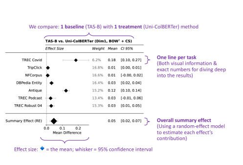
Figure 1: Example forest plot, with explanations highlighting the output of our Ranger toolkit for a multi-task meta-analysis using effect sizes between a control baseline and treatment methods (In this case we use experiments from ColBERTer Hofstätter et al. (2022)).

2 Related Work

In the last years, increasingly more issues of benchmarking have been discussed in NLP Church et al. (2021); Colombo et al. (2022) and IR Craswell et al. (2022); Voorhees and Roberts (2021). Bowman and Dahl (2021) raise the issue that unreliable and biased systems score disproportionately high on benchmarks in Natural Language Understanding and that constructing adversarial, out-of-distribution test sets also only hides the abilities that the benchmarks should measure. Bowman (2022) notice that the now common practices for evaluation lead to unreliable, unrealistically positive claims about the systems. In IR one common multi-task benchmark is BEIR Thakur et al. (2021), which evaluates retrieval models on multiple tasks and domains, however in the evaluation the overall effect of a model is measured by averaging the nDCG scores over each task. As the nDCG score is task dependent and can only be compared within one task, it can not be averaged over different tasks and the mean of the nDCG scores does not hold any meaning. Thus there is the urgent need in the NLP and IR community for a robust, synthesized statistical evaluation over multiple tasks, which is able to aggregate scores, which are not comparable, to an overall effect.

To address these needs Soboroff (2018) propose effect-size based meta-analysis with the use case of evaluation in IR for a robust, aggregated evaluation over multiple tasks. Similarily, Colombo et al. (2022) propose a new method for ranking systems based on their performance across different tasks based on theories of social choice.

In NLP and IR research exist numerous single evaluation tools Azzopardi et al. (2019); MacAvaney et al. (2022), however to the best of our knowledge there exists no evaluation tool addressing the needs for robust, synthesized multi-task evaluation based on meta-analysis.

In order to make this robust, effect-size based evaluation easily accessible for a broad range of tasks, we present our Ranger toolkit and demonstrate use cases in NLP and IR.

3 Ranger

3.1 Methodology

Besides analyzing the effects in individual studies, meta-analysis aims to summarize those effects in one statistical synthesis Borenstein et al. (2009). Translated to the use case of NLP and IR, meta-analysis is a tool to compare whether a treatment model yields gains over a control model within different data collections and overall Soboroff (2018). A treatment, for example, could be an incremental update to the control model, a new model, or a model trained with additional data; a control model can be considered as the baseline (e.g., current SOTA, etc.) to compare the treatment with. To conduct a meta-analysis, defining an effect size is necessary. In this work, we quantify the effect size utilizing the raw mean difference, the standardized mean difference, and the correlation. In particular, we implement the definitions of those effect sizes as defined by Borenstein et al. (2009) for paired study designs since, typically, the compared metrics in IR and NLP experiments are obtained by employing treatment and control models on the same collections.

Raw Mean Difference $D$.

In IR and NLP experiments, researchers usually obtain performance metrics for every item in a collection. By comparing the average of these metrics, they can make statements about the relative performance of different models. Thus, the difference in means is a simple and easy-to-interpret measure of the effect size, as it is on the same scale as the underlying metric. We compute the raw mean difference $D$ by averaging the pairwise differences between treatment $X_{T}$ and control metric $X_{C}$ and use the standard deviation ($S_{diff}$) of the pairwise differences to compute its corresponding variance $V_{D}$ as follows:

$$\begin{split}D&=\frac{X_{T}-X_{C}}{n},\\ V_{D}&=\frac{S^{2}_{diff}}{n},\\ \end{split}$$ (1)

where $n$ is the number of compared pairs.

Standardized Mean Difference $d$.

Sometimes, we might consider standardizing the mean difference (i.e., transforming it into a “unitless” form) to make the effect size comparable and combinable across studies. For example, if a benchmark computes accuracy differently in its individual collections or employs different ranking metrics. The standardized mean difference is computed by dividing the raw mean difference $D$ by the within-group standard deviation $S_{within}$ calculated across the treatment and control metrics.

$$d=\frac{D}{S_{within}}$$ (2)

Having the standard deviation of the pairwise differences $S_{diff}$ and the correlation of the corresponding pairs $r$, we compute $S_{within}$ as follows:

$$S_{within}=\frac{S_{diff}}{\sqrt{2(1-r)}}$$ (3)

The variance of standardized mean difference $d$ is

$$V_{d}=(\frac{1}{n}+\frac{d^{2}}{2n})2(1-r),$$ (4)

where $n$ is the number of compared pairs. In small samples, $d$ tends to overestimate the absolute value of the true standardized mean difference $\delta$, which can be corrected by factor $J$ to obtain an unbiased estimate called Hedges’ $g$ Hedges (1981); Borenstein et al. (2009) and its corresponding variance$V_{g}$:

$$\begin{split}J&=1-\frac{3}{4df-1},\\ g&=J\times d,\\ V_{g}&=J^{2}\times V_{d},\end{split}$$ (5)

where $df$ is degrees of freedom which is $n-1$ in the paired study setting with $n$ number of pairs.

Correlation $r$.

Some studies might utilize the correlation coefficient as an evaluation metric, for example, how the output of an introduced model (treatment) correlates with a certain gold standard (control). In such cases, the correlation coefficient itself can serve as the effect size, and its variance is approximated as follows:

$$V_{r}=\frac{(1-r^{2})^{2}}{n-1},$$ (6)

where $n$ is the sample size. Since the variance strongly depends on the correlation, the correlation coefficient is typically converted to Fisher’s $z$ scale to conduct a meta-analysis Borenstein et al. (2009). The transformation and corresponding variance is:

$$\begin{split}z&=0.5\times ln(\frac{1+r}{1-r}),\\ V_{z}&=\frac{1}{n-3}\end{split}$$ (7)

As already mentioned, $z$ and $V_{z}$ are used throughout the meta-analysis; however, for reporting/communication, $z$ metrics are transformed back into the correlation scale using:

$$r=\frac{e^{2z}-1}{e^{2z}+1}$$ (8)

Combined Effect $M^{*}$.

After calculating the individual effect sizes ($Y_{i}$) and corresponding variances ($V_{Y_{i}}$) for a group of $k$ experiments, the final step in meta-analysis is to merge them into a single summary effect. As Soboroff (2018), we assume heterogeneity, i.e., that the effect size variance varies across the experiments. Following Soboroff (2018), we employ the random-effects model as defined in Borenstein et al. (2009) to consider the between-study variance $T^{2}$ for the summary effect computation. We use the DerSimonian and Laird method DerSimonian and Laird (2015) to estimate $T^{2}$:

$$\begin{split}T^{2}&=\frac{Q-df}{C},\\ Q&=\sum^{k}_{i=1}W_{i}Y^{2}_{i}-\frac{(\sum^{k}_{i=1}W_{i}Y^{2}_{i})^{2}}{\sum^{k}_{i=1}W_{i}},\\ df&=k-1,\\ C&=\sum W_{i}-\frac{\sum W^{2}_{i}}{\sum W_{i}}.\end{split}$$ (9)

where the weight of the individual experiments $W_{i}=1/V_{Y_{i}}$. We adjust the weights by $T^{2}$ and compute the weighted average of the individual effect sizes, i.e., the summary effect $M^{*}$, and its corresponding variance $V_{M^{*}}$ as follows:

$$\begin{split}W^{*}_{i}&=\frac{1}{V_{Y_{i}}+T^{2}},\\ M^{*}&=\frac{\sum^{k}_{i=1}W^{*}_{i}Y_{i}}{\sum^{k}_{i=1}W^{*}_{i}},\\ V_{M^{*}}&=\frac{1}{\sum^{k}_{i=1}W^{*}_{i}}.\end{split}$$ (10)

Confidence Interval (CI).

We determine the corresponding confidence interval (represented by the lower limit, $LL_{Y}$, and the upper limit, $UL_{Y}$) for a given effect size $Y$, which can be the result of an individual experiment ($Y_{i}$) or the summary effect ($M^{*}$), as follows:

$$\begin{split}SE_{Y}&=\sqrt{V_{Y}},\\ LL_{Y}&=Y-Z^{\alpha}\times SE_{Y},\\ UL_{Y}&=Y+Z^{\alpha}\times SE_{Y},\end{split}$$ (11)

where $SE_{Y}$ is the standard error, $V_{Y}$ the variance of the effect size, and $Z^{\alpha}$ the Z-value corresponding to the desired significance level $\alpha$. Given $\alpha$ we compute $Z^{\alpha}$:

$$Z^{\alpha}=ppf(1-\frac{\alpha}{2}),$$ (12)

where $ppf()$ is the percent point function (we use scipy.stats.norm.ppf). For example, $\alpha=0.05$ yields the 95% CI of $Y\pm 1.96\times SE_{Y}$.

Forest Plots.

The meta-analysis results in the individual experiments’ effect sizes, a statistical synthesis of them, and their corresponding confidence intervals. Forest plots are a convenient way of reporting those results, which enables a very intuitive interpretation at one glance. Ranger supports forest plots out of the box, which can easily be customized to one’s needs since it is based on python and matplotlib. We provide an example with explanations in Figure 1. Effect sizes and corresponding confidence intervals are depicted as diamonds with whiskers $\vdash\blacklozenge\dashv$. The size of the diamonds is scaled by the experiments’ weights ($W^{*}_{i}$). The dotted vertical line $\vdots$ at zero represents the zero effect. The observed effect size is not significant when its confidence interval crosses the zero effect line; in other words, we cannot detect the effect size at the given confidence level.

3.2 Usage

We explain the easy usage of Ranger along with two examples on classification evaluation of GLUE in NLP and retrieval evaluation of BEIR in IR.

The meta-analysis with Ranger requires as input either 1) a text file already containing the sample-wise metrics for each task (in the GLUE example) or 2) a text file containing the retrieval runs and the qrels containing the labels (in the BEIR example).

The paths to the text files for each task are stored in a config.yaml file and read in with the class ClassificationLocationConfig or RetrievalLocationConfig. The entry point for loading the data and possibly computing metrics is load_and_compute_metrics(name, measure, config). Having the treatment and control data, we can analyze the effects and compute effect sizes:

⬇

from ranger.metric_containers import

AggregatedPairedMetrics, AggregatedMetrics

from ranger.meta_analysis import

analyze_effects

\pareffects = AggregatedPairedMetrics(

treatment=t.get_metrics(),

control=c.get_metrics())

eff_size = analyze_effects(

list(conf.display_names.values()),

effects=effects,

effect_type="SMD")

Here the effect_type variable refers to the type of difference measurement in the meta-analysis as introduced in the previous section. The choice is between Raw Mean differences ("MD"), standardized mean differences ("SMD") or correlation ("CORR"). In order to visualize the effects, Ranger produces beautiful forest plots:

⬇

from ranger.forest_plots import forest_plot

\parplot = forest_plot(title=title,

experiment_names=list(config.display_names

.values()),

label_x_axis="Standardized Mean Difference",

effect_size=eff_size,

fig_width=8,

fig_height=8)

4 Case Study NLP: GLUE benchmark

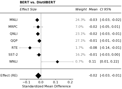
Figure 2: Forest plot of Ranger toolkit for tasks of the GLUE benchmark. Comparison in terms of accuracy between BERT and DistilBERT.

In order to demonstrate the usage of the Ranger toolkit for various multi-task benchmarks, we conduct an evaluation on the popular General Language Understanding (GLUE) Benchmark Wang et al. (2018).

We train and compare two classifiers on the GLUE benchmark: one classifier based on BERT Devlin et al. (2018), the latter based on a smaller, more efficient transformer model trained on BERT scores, namely DistilBERT Sanh et al. (2019) .

The official evaluation metric for two of the nine tasks (for CoLA and STS-B) is a correlation-based metric. Since these correlation-based metrics can not be computed sample-wise for each sample in the test set, the effect-size based meta-analysis can not be applied to those metrics and we exclude these two tasks from our evaluation.

We conduct the effect-size based meta-analysis based on the accuracy as metric and use Standardized Mean Difference to measure the effect-size (type in Ranger toolkit is ’SMD’). We illustrate the meta-analysis of the BERT and DistilBERT classifier in Figure 2. We also publish the Walk-you-Through Jupyter notebook in the Ranger toolkit to attain this forest plot for GLUE.

The location of the black diamonds visualizes the effect of the treatment (DistilBERT) compared to the baseline (BERT), whereas the size of the diamonds refers to the weight of this effect in the overall summary effect. We can see that using DistilBERT as base model for the classifier compared to BERT, has overall effect of a minor decrease in effectiveness. This behaviour is similar with the results on the MNLI, QNLI, and QQP where we also notice that the confidence intervals are very narrow or even non existent in the forest plot. For MRPC and SST-2 there is also a negative effect, however the effect is not significant, since the confidence intervals overlap with the baseline performance. For RTE and WNLI the effect of using DistilBERT compared to BERT is rather big compared to the summary effect, where for RTE the mean is 8% lower and for WNLI the mean is 11% higher than for the BERT classifier. However the large confidence intervals of these tasks indicate the large variability in the effect and thus the weight for taking these effects into account in the summary effect are rather low (0.7% and 1.7%).

Overall the summary effect shows that the DistilBERT classifier decreases effectiveness consistently by 2%. Since the confidence intervals are so narrow for the overall effect and do not overlap with the baseline (BERT classifier), we see that the overall effect is also significant.

5 Case Study IR: BEIR benchmark

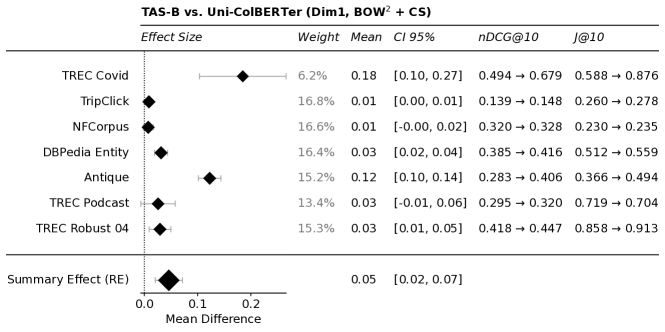
Figure 3: Forest plot of Ranger toolkit for tasks of the BEIR benchmark. Comparison in terms of nDCG@10 between TAS-B and ColBERTer.

Especially in IR evaluation, where it is common to evaluate multiple tasks with metrics, which are not comparable over different tasks Thakur et al. (2021), we see a great benefit of using Ranger to aggregate the results of multiple tasks into one comparable statistical analysis. Thus we demonstrate the case study of using the Ranger toolkit for evaluation on commonly used IR collections, including a subset of the BEIR benchmark Thakur et al. (2021). We presented this study originally as part of Hofstätter et al. (2022), and the Ranger toolkit is a direct descendent of these initial experiments.

We select tasks, which either 1) were annotated at a TREC track and thus contain high quality judgements, 2) were annotated according to the Cranfield paradigm Cleverdon (1967) or 3) contain a large amount of labels. All collections are evaluated with the ranking metric nDCG@10. We compare zero-shot retrieval with TAS-B Hofstätter et al. (2021) as baseline to retrieval with Uni-ColBERTer Hofstätter et al. (2022) as treatment.

We conduct a meta-analysis of the evaluation results based on nDCG@10 as metric and measure the effect-size with the mean difference (type is ’MD’). The output of the Ranger toolkit is illustrated in Figure 3. We publish a walk-through Jupyter notebook in the Ranger toolkit to attain this forest plot for BEIR benchmark evaluation.

In Figure 3 the effect size, the weight of the effect on the overall effect as well as the mean and confidence intervals of the effect are visualized. As an extension for IR we also visualize the nDCG@10 performance and J@10 judgement ratio from baseline $\rightarrow$ to treatment.

For NFCorpus and TREC Podcast we see a small positive effect of Uni-ColBERTer compared to TAS-B, however the confidence intervals are overlapping with the baseline performance incdicating no clear positive effect on these tasks. For TripClick, DBPedia Entity and TREC Robust 04 we see a consistent and significant small positive effect with narrow confidence intervals of Uni-ColBERTer and this effect is even greater for Antique and TREC Covid. Notice the great confidence intervals for TREC Covid, since the evaluation of TREC Covid is only based on 50 queries and thus its influence for the overall effect should be and is the lowest (6.2%) among the test sets.

The judgement ratio J@10 in the left most column shows the percentage of judged documents in the Top 10 of retrieved results. Analyzing the judgement ratio one can also get an understanding of how reliable the evaluation results are and how comparable the results of the two different retrieval models are, since a high difference in judgement ratio could indicate lower comparability of the two models with the respective test set.

Overall the summary effect of Uni-ColBERTer compared to TAS-B is consistent and significantly positive, increasing effectiveness by 0.05.

6 Conclusion

We presented Ranger – a task-agnostic toolkit for easy-to-use meta-analysis to evaluate multiple tasks. We described the theoretical basis on which we built our toolkit; the implementation and usage; and furthermore we provide two cases studies for common IR and NLP settings to highlight capabilities of Ranger. We do not claim to have all the answers, nor that using Ranger will solve all your multi-task evaluation problems. Nevertheless, we hope that Ranger is useful for the community to improve multi-task experimentation and make its evaluation more robust.

Acknowledgements

This work is supported by the Christian Doppler Research Association (CDG) and has received funding from the EU Horizon 2020 ITN/ETN project on Domain Specific Systems for Information Extraction and Retrieval (H2020-EU.1.3.1., ID: 860721).

References

- Azzopardi et al. (2019) Leif Azzopardi, Paul Thomas, and Alistair Moffat. 2019. Cwl_eval: An evaluation tool for information retrieval. In Proceedings of the 42nd International ACM SIGIR Conference on Research and Development in Information Retrieval, SIGIR’19, page 1321–1324, New York, NY, USA. Association for Computing Machinery.
- Borenstein et al. (2009) Michael Borenstein, Larry V Hedges, Julian PT Higgins, and Hannah R Rothstein. 2009. Introduction to meta-analysis. John Wiley & Sons, Ltd.
- Bowman (2022) Samuel Bowman. 2022. The dangers of underclaiming: Reasons for caution when reporting how NLP systems fail. In Proceedings of the 60th Annual Meeting of the Association for Computational Linguistics (Volume 1: Long Papers), pages 7484–7499, Dublin, Ireland. Association for Computational Linguistics.
- Bowman and Dahl (2021) Samuel R. Bowman and George Dahl. 2021. What will it take to fix benchmarking in natural language understanding? In Proceedings of the 2021 Conference of the North American Chapter of the Association for Computational Linguistics: Human Language Technologies, pages 4843–4855, Online. Association for Computational Linguistics.
- Church et al. (2021) Kenneth Church, Mark Liberman, and Valia Kordoni. 2021. Benchmarking: Past, present and future. In Proceedings of the 1st Workshop on Benchmarking: Past, Present and Future, pages 1–7, Online. Association for Computational Linguistics.
- Cleverdon (1967) Cyril Cleverdon. 1967. The Cranfield Tests on Index Language Devices. San Francisco, CA, USA.
- Colombo et al. (2022) Pierre Colombo, Nathan Noiry, Ekhine Irurozki, and Stephan Clémençon. 2022. What are the best systems? new perspectives on nlp benchmarking. In Advances in Neural Information Processing Systems, volume 35, pages 26915–26932. Curran Associates, Inc.
- Craswell et al. (2022) Nick Craswell, Bhaskar Mitra, Emine Yilmaz, Daniel Campos, and Jimmy Lin. 2022. Overview of the trec 2021 deep learning track. In Text REtrieval Conference (TREC). TREC.
- DerSimonian and Laird (2015) Rebecca DerSimonian and Nan Laird. 2015. Meta-analysis in clinical trials revisited. Contemporary Clinical Trials, 45:139–145. 10th Anniversary Special Issue.
- Devlin et al. (2018) Jacob Devlin, Ming-Wei Chang, Kenton Lee, and Kristina Toutanova. 2018. Bert: Pre-training of deep bidirectional transformers for language understanding. arXiv preprint arXiv:1810.04805.
- Hedges (1981) Larry V Hedges. 1981. Distribution theory for glass’s estimator of effect size and related estimators. journal of Educational Statistics, 6(2):107–128.
- Hofstätter et al. (2022) Sebastian Hofstätter, Omar Khattab, Sophia Althammer, Mete Sertkan, and Allan Hanbury. 2022. Introducing neural bag of whole-words with colberter: Contextualized late interactions using enhanced reduction.
- Hofstätter et al. (2021) Sebastian Hofstätter, Sheng-Chieh Lin, Jheng-Hong Yang, Jimmy Lin, and Allan Hanbury. 2021. Efficiently Teaching an Effective Dense Retriever with Balanced Topic Aware Sampling. In Proceedings of the 44rd International ACM SIGIR Conference on Research and Development in Information Retrieval (SIGIR ’21).
- MacAvaney et al. (2022) Sean MacAvaney, Craig Macdonald, and Iadh Ounis. 2022. Streamlining evaluation with ir-measures. In Advances in Information Retrieval: 44th European Conference on IR Research, ECIR 2022, Stavanger, Norway, April 10–14, 2022, Proceedings, Part II, page 305–310, Berlin, Heidelberg. Springer-Verlag.
- Sanh et al. (2019) Victor Sanh, Lysandre Debut, Julien Chaumond, and Thomas Wolf. 2019. Distilbert, a distilled version of bert: smaller, faster, cheaper and lighter. arXiv preprint arXiv:1910.01108.
- Soboroff (2018) Ian Soboroff. 2018. Meta-analysis for retrieval experiments involving multiple test collections. In Proc. of CIKM.
- Thakur et al. (2021) Nandan Thakur, Nils Reimers, Andreas Rücklé, Abhishek Srivastava, and Iryna Gurevych. 2021. Beir: A heterogenous benchmark for zero-shot evaluation of information retrieval models.
- Voorhees and Roberts (2021) Ellen M. Voorhees and Kirk Roberts. 2021. On the quality of the TREC-COVID IR test collections. In SIGIR ’21: The 44th International ACM SIGIR Conference on Research and Development in Information Retrieval, Virtual Event, Canada, July 11-15, 2021, pages 2422–2428. ACM.
- Wang et al. (2018) Alex Wang, Amanpreet Singh, Julian Michael, Felix Hill, Omer Levy, and Samuel Bowman. 2018. GLUE: A multi-task benchmark and analysis platform for natural language understanding. In Proceedings of the 2018 EMNLP Workshop BlackboxNLP: Analyzing and Interpreting Neural Networks for NLP, pages 353–355, Brussels, Belgium. Association for Computational Linguistics.