Electric $1^{+}$ state below nuclear scissors

Abstract

The solution of time dependent Hartree-Fock-Bogoliubov equations by the Wigner function moments method predicts four low-lying $1^{+}$ states. Three of them are known as various scissors modes. Fourth state is disposed below all scissors modes and has the electrical nature. It is found that it represents one of three branches of $2^{+}$ state which can exist in spherical nuclei and which is split in deformed nuclei. It is discovered, that the antiferromagnetic properties of nuclei lead to the splitting of $2^{+}$ states already at the zero deformation.

I Introduction

The theoretical interpretation of collective nuclear dynamics, realized through electromagnetic transitions in the low-energy region, is one of the most interesting topics in nuclear structure physics. The method of Wigner function moments (WFM) or phase space moments turned out to be very convenient to describe the collective excitations of nuclei. On the one hand, this is a purely microscopic approach, since it is based on the non-stationary Hartree-Fock-Bogolyubov equation. On the other hand, the method works with average values (moments) of operators, which have a transparent physical meaning, and their dynamics is directly related to the processes under consideration. Thus, a natural bridge is thrown over with a macroscopic description. All this makes the WFM method an ideal instrument for describing the main characteristics (energies and excitation probabilities) of collective excitations.

The description of the collective motion of nuclei in terms of WFM was first proposed in 1981 Ba81 . It has been successfully applied to study giant multipole resonances and low-lying collective modes of rotating and non-rotating nuclei with different realistic forces Ba91 ; BaMo94 . The catalyst for further progression along this path of research was the understanding of the conceptual closeness of the WFM method and the variances-covariances approach developed by Peter Schuck Sc84 . This formed the basis for joining efforts in this common direction of research. Initially, the method was applied to the study of large amplitude motion. Its Fourier analysis gave a lot of information about the variety of multiphonon states of nuclei BaSc97 ; BaSc99 .

A significant point in the study of the nature of collective vibrations was the idea of orbital scissors, first reported by R. Hilton in 1976 at the conference on nuclear structure in Dubna Hilt . This idea was subsequently developed in the works of Suzuki and Rowe Suzuki , Lo Iudice and Palumbo LoIP78 and other authors. The first experimental detection of the nuclear scissors in ¹⁵⁶Gd by the Darmstadt group Bohle has initiated a cascade of experimental and theoretical studies. An exhaustive review of the subject is given in the paper Heyd containing about 400 references.

The detailed analysis of the scissors mode in the framework of a solvable model (harmonic oscillator with quadrupole-quadrupole residual interaction) was given in BaSc . These investigations have shown that in the small-amplitude approximation, already the minimal set of collective variables, i.e. phase space moments up to quadratic order, is sufficient to reproduce the most important property of the scissors mode: its inevitable coexistence with the isovector Giant Quadrupole Resonance (GQR) implying a deformation of the Fermi surface. Additionally, this simple model, which allows one to obtain exact analytical solutions, proved to be a good basis for studying the interrelation between WFM method and Random Phase Approximation (RPA). It was shown that these two methods give identical formulae for eigenfrequencies and transition probabilities of all collective excitations of the model, including the scissors mode. On the whole, it can be concluded that the second order moment equations yield an optimally coarse grained image of the full QRPA spectrum BaSc06 ; Ann .

The simple model provided a lot of useful information about collective motion, correctly conveyed the observed tendences for scissors mode, and helped to better understand the potential capability of the method of moments and its relationship to microscopics. However, the energy of the scissors mode turned out to be too low, and the values of $B(M1)$ were too large compared to the experimental data. Accounting for pair correlations significantly improved agreement with experiment, but did not completely solve the problem Malov ; Malov1 . It became clear that the spin-orbit interaction must be included in the consideration. In the paper BaMo the WFM method was generalized to solve the TDHF equations including spin dynamics. The most remarkable result was the prediction of a new type of nuclear collective motion: rotational oscillations of ”spin up” nucleons with respect to ”spin down” nucleons (the spin scissors mode). A generalization of the WFM method which takes into account spin degrees of freedom and pair correlations simultaneously was outlined in BaMoPRC2 , where the Time Dependent Hartree-Fock-Bogoliubov (TDHFB) equations were considered. As a result the agreement between theory and experiment in the description of nuclear scissors modes was improved considerably. Furthermore, after taking into account the isovector-isoscalar coupling BaMoPRC22 one more magnetic mode (third type of scissors) emerged. Actually, the possible existence of three scissors motions is easily explained by combinatoric consideration – there are only three ways to divide the four different kinds of objects (spin up and spin down protons and neutrons in our case) into two pairs. The three types of scissors modes can be approximately classified as isovector spin-scalar (conventional), isovector spin-vector and isoscalar spin-vector.

All these results have been obtained through many years of exciting and fruitful collaboration with Peter Schuck, whose intellectual contribution to the development of the WFM method is invaluable.

The WFM based calculations also predict low-lying excitation with large $B(E2)$ and negligible $B(M1)$ values, which is disposed just below all scissors modes. Until now, we have left this topic out of the discussion. The focus of the present work is an analysis of the nature of this state.

II TDHFB equations and WFM equations of motion

The TDHFB equations in matrix formulation Solov ; Ring are

$$i\hbar\dot{\cal R}=[{\cal H},{\cal R}]$$ (1)

with

$${\cal R}={\hat{\rho}\qquad-\hat{\kappa}\choose-\hat{\kappa}^{\dagger}\;\;1-\hat{\rho}^{*}},\quad{\cal H}={\hat{h}\quad\;\;\hat{\Delta}\choose\hat{\Delta}^{\dagger}\quad-\hat{h}^{*}}$$ (2)

The normal density matrix $\hat{\rho}$ and Hamiltonian $\hat{h}$ are hermitian whereas the anomalous density $\hat{\kappa}$ and the pairing gap $\hat{\Delta}$ are skew symmetric: $\hat{\kappa}^{\dagger}=-\hat{\kappa}^{*}$, $\hat{\Delta}^{\dagger}=-\hat{\Delta}^{*}$. The detailed form of the TDHFB equations is

$$i\hbar\dot{\hat{\rho}}=\hat{h}\hat{\rho}-\hat{\rho}\hat{h}-\hat{\Delta}\hat{\kappa}^{\dagger}+\hat{\kappa}\hat{\Delta}^{\dagger},$$

$$-i\hbar\dot{\hat{\rho}}^{*}=\hat{h}^{*}\hat{\rho}^{*}-\hat{\rho}^{*}\hat{h}^{*}-\hat{\Delta}^{\dagger}\hat{\kappa}+\hat{\kappa}^{\dagger}\hat{\Delta},$$

$$-i\hbar\dot{\hat{\kappa}}=-\hat{h}\hat{\kappa}-\hat{\kappa}\hat{h}^{*}+\hat{\Delta}-\hat{\Delta}\hat{\rho}^{*}-\hat{\rho}\hat{\Delta},$$

$$-i\hbar\dot{\hat{\kappa}}^{\dagger}=\hat{h}^{*}\hat{\kappa}^{\dagger}+\hat{\kappa}^{\dagger}\hat{h}-\hat{\Delta}^{\dagger}+\hat{\Delta}^{\dagger}\hat{\rho}+\hat{\rho}^{*}\hat{\Delta}^{\dagger}.$$ (3)

Let us consider their matrix form in coordinate space keeping all spin indices $s,s^{\prime}$: $\langle{\bf r},s|\hat{\rho}|{\bf r}^{\prime},s^{\prime}\rangle$, $\langle{\bf r},s|\hat{\kappa}|{\bf r}^{\prime},s^{\prime}\rangle$, etc. We do not specify the isospin indices in order to make formulae more transparent. After introduction of the more compact notation $\langle{\bf r},s|\hat{X}|{\bf r}^{\prime},s^{\prime}\rangle=X_{rr^{\prime}}^{ss^{\prime}}$ the set of equations (3) with specified spin indices reads

$$i\hbar\dot{\rho}_{rr^{\prime\prime}}^{\uparrow\uparrow}=\int\!d^{3}r^{\prime}(h_{rr^{\prime}}^{\uparrow\uparrow}\rho_{r^{\prime}r^{\prime\prime}}^{\uparrow\uparrow}-\rho_{rr^{\prime}}^{\uparrow\uparrow}h_{r^{\prime}r^{\prime\prime}}^{\uparrow\uparrow}+h_{rr^{\prime}}^{\uparrow\downarrow}\rho_{r^{\prime}r^{\prime\prime}}^{\downarrow\uparrow}-\rho_{rr^{\prime}}^{\uparrow\downarrow}h_{r^{\prime}r^{\prime\prime}}^{\downarrow\uparrow}-\Delta_{rr^{\prime}}^{\uparrow\downarrow}{\kappa^{\dagger}}_{r^{\prime}r^{\prime\prime}}^{\downarrow\uparrow}+\kappa_{rr^{\prime}}^{\uparrow\downarrow}{\Delta^{\dagger}}_{r^{\prime}r^{\prime\prime}}^{\downarrow\uparrow}),$$

$$i\hbar\dot{\rho}_{rr^{\prime\prime}}^{\uparrow\downarrow}=\int\!d^{3}r^{\prime}(h_{rr^{\prime}}^{\uparrow\uparrow}\rho_{r^{\prime}r^{\prime\prime}}^{\uparrow\downarrow}-\rho_{rr^{\prime}}^{\uparrow\uparrow}h_{r^{\prime}r^{\prime\prime}}^{\uparrow\downarrow}+h_{rr^{\prime}}^{\uparrow\downarrow}\rho_{r^{\prime}r^{\prime\prime}}^{\downarrow\downarrow}-\rho_{rr^{\prime}}^{\uparrow\downarrow}h_{r^{\prime}r^{\prime\prime}}^{\downarrow\downarrow}),$$

$$i\hbar\dot{\rho}_{rr^{\prime\prime}}^{\downarrow\uparrow}=\int\!d^{3}r^{\prime}(h_{rr^{\prime}}^{\downarrow\uparrow}\rho_{r^{\prime}r^{\prime\prime}}^{\uparrow\uparrow}-\rho_{rr^{\prime}}^{\downarrow\uparrow}h_{r^{\prime}r^{\prime\prime}}^{\uparrow\uparrow}+h_{rr^{\prime}}^{\downarrow\downarrow}\rho_{r^{\prime}r^{\prime\prime}}^{\downarrow\uparrow}-\rho_{rr^{\prime}}^{\downarrow\downarrow}h_{r^{\prime}r^{\prime\prime}}^{\downarrow\uparrow}),$$

$$i\hbar\dot{\rho}_{rr^{\prime\prime}}^{\downarrow\downarrow}=\int\!d^{3}r^{\prime}(h_{rr^{\prime}}^{\downarrow\uparrow}\rho_{r^{\prime}r^{\prime\prime}}^{\uparrow\downarrow}-\rho_{rr^{\prime}}^{\downarrow\uparrow}h_{r^{\prime}r^{\prime\prime}}^{\uparrow\downarrow}+h_{rr^{\prime}}^{\downarrow\downarrow}\rho_{r^{\prime}r^{\prime\prime}}^{\downarrow\downarrow}-\rho_{rr^{\prime}}^{\downarrow\downarrow}h_{r^{\prime}r^{\prime\prime}}^{\downarrow\downarrow}-\Delta_{rr^{\prime}}^{\downarrow\uparrow}{\kappa^{\dagger}}_{r^{\prime}r^{\prime\prime}}^{\uparrow\downarrow}+\kappa_{rr^{\prime}}^{\downarrow\uparrow}{\Delta^{\dagger}}_{r^{\prime}r^{\prime\prime}}^{\uparrow\downarrow}),$$

$$i\hbar\dot{\kappa}_{rr^{\prime\prime}}^{\uparrow\downarrow}=-\Delta_{rr^{\prime\prime}}^{\uparrow\downarrow}+\int\!d^{3}r^{\prime}\left(h_{rr^{\prime}}^{\uparrow\uparrow}\kappa_{r^{\prime}r^{\prime\prime}}^{\uparrow\downarrow}+\kappa_{rr^{\prime}}^{\uparrow\downarrow}{h^{*}}_{r^{\prime}r^{\prime\prime}}^{\downarrow\downarrow}+\Delta_{rr^{\prime}}^{\uparrow\downarrow}{\rho^{*}}_{r^{\prime}r^{\prime\prime}}^{\downarrow\downarrow}+\rho_{rr^{\prime}}^{\uparrow\uparrow}\Delta_{r^{\prime}r^{\prime\prime}}^{\uparrow\downarrow}\right),$$

$$i\hbar\dot{\kappa}_{rr^{\prime\prime}}^{\downarrow\uparrow}=-\Delta_{rr^{\prime\prime}}^{\downarrow\uparrow}+\int\!d^{3}r^{\prime}\left(h_{rr^{\prime}}^{\downarrow\downarrow}\kappa_{r^{\prime}r^{\prime\prime}}^{\downarrow\uparrow}+\kappa_{rr^{\prime}}^{\downarrow\uparrow}{h^{*}}_{r^{\prime}r^{\prime\prime}}^{\uparrow\uparrow}+\Delta_{rr^{\prime}}^{\downarrow\uparrow}{\rho^{*}}_{r^{\prime}r^{\prime\prime}}^{\uparrow\uparrow}+\rho_{rr^{\prime}}^{\downarrow\downarrow}\Delta_{r^{\prime}r^{\prime\prime}}^{\downarrow\uparrow}\right).$$ (4)

with the conventional notation

$$\uparrow\,\mbox{for}\quad s=\frac{1}{2}\quad\mbox{and}\quad\downarrow\,\mbox{for}\quad s=-\frac{1}{2}.$$

This set of equations must be complemented by the complex conjugated equations. Writing these equations we neglected the diagonal in spin matrix elements of the anomalous density: $\kappa_{rr^{\prime}}^{ss}$ and $\Delta_{rr^{\prime}}^{ss}$. It was shown in BaMoPRC2 that such an approximation works very well in the case of monopole pairing considered here.

We will consider the Wigner transform Ring of equations (4) (see Malov ; Malov1 for mathematical details). So, instead of four (in $ss^{\prime}$) matrix elements of the density matrix $\rho_{rr^{\prime}}^{ss^{\prime}}$ and two matrix elements $\kappa_{rr^{\prime}}^{\uparrow\downarrow}$, $\kappa_{rr^{\prime}}^{\downarrow\uparrow}$ we will consider four Wigner functions $f^{ss^{\prime}}({\bf r},{\bf p})$ and two phase space distributions $\kappa^{ss^{\prime}}({\bf r},{\bf p})$, that is more convenient for WFM method (see BaMoPRC2 ; BaMoPRC22 for details). From now on, we will not write out the coordinate dependence $({\bf r},{\bf p})$ of all functions in order to make the formulae more transparent. We have

$$i\hbar\dot{f}^{\uparrow\uparrow} = i\hbar\{h^{\uparrow\uparrow},f^{\uparrow\uparrow}\}+h^{\uparrow\downarrow}f^{\downarrow\uparrow}-f^{\uparrow\downarrow}h^{\downarrow\uparrow}+\frac{i\hbar}{2}\{h^{\uparrow\downarrow},f^{\downarrow\uparrow}\}-\frac{i\hbar}{2}\{f^{\uparrow\downarrow},h^{\downarrow\uparrow}\}$$

$$- \frac{\hbar^{2}}{8}\{\!\{h^{\uparrow\downarrow},f^{\downarrow\uparrow}\}\!\}+\frac{\hbar^{2}}{8}\{\!\{f^{\uparrow\downarrow},h^{\downarrow\uparrow}\}\!\}+\kappa\Delta^{*}-\Delta\kappa^{*}$$

$$+ \frac{i\hbar}{2}\{\kappa,\Delta^{*}\}-\frac{i\hbar}{2}\{\Delta,\kappa^{*}\}-\frac{\hbar^{2}}{8}\{\!\{\kappa,\Delta^{*}\}\!\}+\frac{\hbar^{2}}{8}\{\!\{\Delta,\kappa^{*}\}\!\}+...,$$

$$i\hbar\dot{f}^{\downarrow\downarrow} = i\hbar\{h^{\downarrow\downarrow},f^{\downarrow\downarrow}\}+h^{\downarrow\uparrow}f^{\uparrow\downarrow}-f^{\downarrow\uparrow}h^{\uparrow\downarrow}+\frac{i\hbar}{2}\{h^{\downarrow\uparrow},f^{\uparrow\downarrow}\}-\frac{i\hbar}{2}\{f^{\downarrow\uparrow},h^{\uparrow\downarrow}\}$$

$$- \frac{\hbar^{2}}{8}\{\!\{h^{\downarrow\uparrow},f^{\uparrow\downarrow}\}\!\}+\frac{\hbar^{2}}{8}\{\!\{f^{\downarrow\uparrow},h^{\uparrow\downarrow}\}\!\}+\bar{\Delta}^{*}\bar{\kappa}-\bar{\kappa}^{*}\bar{\Delta}$$

$$+ \frac{i\hbar}{2}\{\bar{\Delta}^{*},\bar{\kappa}\}-\frac{i\hbar}{2}\{\bar{\kappa}^{*},\bar{\Delta}\}-\frac{\hbar^{2}}{8}\{\!\{\bar{\Delta}^{*},\bar{\kappa}\}\!\}+\frac{\hbar^{2}}{8}\{\!\{\bar{\kappa}^{*},\bar{\Delta}\}\!\}+...,$$

$$i\hbar\dot{f}^{\uparrow\downarrow} = f^{\uparrow\downarrow}h^{-}+\frac{i\hbar}{2}\{h^{+},f^{\uparrow\downarrow}\}-\frac{\hbar^{2}}{8}\{\!\{h^{-},f^{\uparrow\downarrow}\}\!\}$$

$$- h^{\uparrow\downarrow}f^{-}+\frac{i\hbar}{2}\{h^{\uparrow\downarrow},f^{+}\}+\frac{\hbar^{2}}{8}\{\!\{h^{\uparrow\downarrow},f^{-}\}\!\}+....,$$

$$i\hbar\dot{f}^{\downarrow\uparrow} = -f^{\downarrow\uparrow}h^{-}+\frac{i\hbar}{2}\{h^{+},f^{\downarrow\uparrow}\}+\frac{\hbar^{2}}{8}\{\!\{h^{-},f^{\downarrow\uparrow}\}\!\}$$

$$+ h^{\downarrow\uparrow}f^{-}+\frac{i\hbar}{2}\{h^{\downarrow\uparrow},f^{+}\}-\frac{\hbar^{2}}{8}\{\!\{h^{\downarrow\uparrow},f^{-}\}\!\}+...,$$

$$i\hbar\dot{\kappa} = \kappa\,(h^{\uparrow\uparrow}+\bar{h}^{\downarrow\downarrow})+\frac{i\hbar}{2}\{(h^{\uparrow\uparrow}-\bar{h}^{\downarrow\downarrow}),\kappa\}-\frac{\hbar^{2}}{8}\{\!\{(h^{\uparrow\uparrow}+\bar{h}^{\downarrow\downarrow}),\kappa\}\!\}$$

$$+ \Delta\,(f^{\uparrow\uparrow}+\bar{f}^{\downarrow\downarrow})+\frac{i\hbar}{2}\{(f^{\uparrow\uparrow}-\bar{f}^{\downarrow\downarrow}),\Delta\}-\frac{\hbar^{2}}{8}\{\!\{(f^{\uparrow\uparrow}+\bar{f}^{\downarrow\downarrow}),\Delta\}\!\}-\Delta+...,$$

$$i\hbar\dot{\kappa}^{*} = -\kappa^{*}(h^{\uparrow\uparrow}+\bar{h}^{\downarrow\downarrow})+\frac{i\hbar}{2}\{(h^{\uparrow\uparrow}-\bar{h}^{\downarrow\downarrow}),\kappa^{*}\}+\frac{\hbar^{2}}{8}\{\!\{(h^{\uparrow\uparrow}+\bar{h}^{\downarrow\downarrow}),\kappa^{*}\}\!\}$$ (5)

$$- \Delta^{*}(f^{\uparrow\uparrow}+\bar{f}^{\downarrow\downarrow})+\frac{i\hbar}{2}\{(f^{\uparrow\uparrow}-\bar{f}^{\downarrow\downarrow}),\Delta^{*}\}+\frac{\hbar^{2}}{8}\{\!\{(f^{\uparrow\uparrow}+\bar{f}^{\downarrow\downarrow}),\Delta^{*}\}\!\}+\Delta^{*}+...,\qquad$$

where the functions $h^{s,s^{\prime}}({\bf r},{\bf p})$, $f^{s,s^{\prime}}({\bf r},{\bf p})$, $\Delta^{s,s^{\prime}}({\bf r},{\bf p})$, and $\kappa^{s,s^{\prime}}({\bf r},{\bf p})$ are the Wigner transforms of $h^{s,s^{\prime}}_{r,r^{\prime}}$, $\rho^{s,s^{\prime}}_{r,r^{\prime}}$, $\Delta^{s,s^{\prime}}_{r,r^{\prime}}$, and $\kappa^{s,s^{\prime}}_{r,r^{\prime}}$, respectively, $\bar{f}({\bf r},{\bf p})=f({\bf r},-{\bf p})$, $\{f,g\}$ is the Poisson bracket of the functions $f({\bf r},{\bf p})$ and $g({\bf r},{\bf p})$, $\{\{f,g\}\}$ is their double Poisson bracket, $f^{\pm}=f^{\uparrow\uparrow}{\pm}f^{\downarrow\downarrow}$ and $h^{\pm}=h^{\uparrow\uparrow}\pm h^{\downarrow\downarrow}$. The dots stand for terms proportional to higher powers of $\hbar$ – after integration over phase space these terms disappear and we arrive to the set of exact integral equations. This set of equations must be complemented by the dynamical equations for $\bar{f}^{\uparrow\uparrow},\bar{f}^{\downarrow\downarrow},\bar{f}^{\uparrow\downarrow},\bar{f}^{\downarrow\uparrow},\bar{\kappa},\bar{\kappa}^{*}$. They are obtained by the change ${\bf p}\rightarrow-{\bf p}$ in arguments of functions and Poisson brackets. So, in reality we deal with the set of twelve equations. We introduced the notation $\kappa\equiv\kappa^{\uparrow\downarrow}$ and $\Delta\equiv\Delta^{\uparrow\downarrow}$. Symmetry properties of matrices $\hat{\kappa},\hat{\Delta}$ and the properties of their Wigner transforms allow one to replace the functions $\kappa^{\downarrow\uparrow}({\bf r},{\bf p})$ and $\Delta^{\downarrow\uparrow}({\bf r},{\bf p})$ by the functions $\bar{\kappa}^{\uparrow\downarrow}({\bf r},{\bf p})$ and $\bar{\Delta}^{\uparrow\downarrow}({\bf r},{\bf p})$.

The microscopic Hamiltonian of the model, harmonic oscillator with spin orbit potential plus separable quadrupole-quadrupole and spin-spin residual interactions is given by

$$H=\sum\limits_{i=1}^{A}\left[\frac{\hat{\bf p}_{i}^{2}}{2m}+\frac{1}{2}m\omega^{2}{\bf r}_{i}^{2}-\eta\hat{\bf l}_{i}\hat{\bf S}_{i}\right]+H_{qq}+H_{ss},$$ (6)

with

$$H_{qq}=\!\sum_{\mu=-2}^{2}(-1)^{\mu}\left\{\bar{\kappa}\sum\limits_{i}^{Z}\!\sum\limits_{j}^{N}+\frac{\kappa}{2}\left[\sum\limits_{i,j(i\neq j)}^{Z}+\sum\limits_{i,j(i\neq j)}^{N}\right]\right\}q_{2-\mu}({\bf r}_{i})q_{2\mu}({\bf r}_{j}),$$ (7)

$$H_{ss}=\!\sum_{\mu=-1}^{1}(-1)^{\mu}\left\{\bar{\chi}\sum\limits_{i}^{Z}\!\sum\limits_{j}^{N}+\frac{\chi}{2}\left[\sum\limits_{i,j(i\neq j)}^{Z}+\sum\limits_{i,j(i\neq j)}^{N}\right]\right\}\hat{S}_{-\mu}(i)\hat{S}_{\mu}(j)\,\delta({\bf r}_{i}-{\bf r}_{j}),$$ (8)

where $\displaystyle q_{2\mu}({\bf r})=\sqrt{16\pi/5}\,r^{2}Y_{2\mu}(\theta,\phi)=\sqrt{6}\{r\otimes r\}_{2\mu},$ $\{r\otimes r\}_{\lambda\mu}=\sum_{\sigma,\nu}C_{1\sigma,1\nu}^{\lambda\mu}r_{\sigma}r_{\nu},$ $C_{1\sigma,1\nu}^{\lambda\mu}$ is the Clebsch-Gordan coefficient, cyclic coordinates $r_{-1},r_{0},r_{1}$ are defined in Var , $N$ and $Z$ are the numbers of neutrons and protons. $\hat{S}_{\mu}$ are spin matrices Var :

$$\hat{S}_{1}=-\frac{\hbar}{\sqrt{2}}{0\quad 1\choose 0\quad 0},\ \hat{S}_{0}=\frac{\hbar}{2}{1\quad\,0\choose 0\,-\!1},\ \hat{S}_{-1}=\frac{\hbar}{\sqrt{2}}{0\quad 0\choose 1\quad 0}.$$

The mean field generated by this Hamiltonian was derived in BaMoPRC13 .

Equations (5) will be solved in a small amplitude approximation by the WFM method. Integrating them over phase space with the weights

$$W=\{r\otimes p\}_{\lambda\mu},\,\{r\otimes r\}_{\lambda\mu},\,\{p\otimes p\}_{\lambda\mu},\mbox{ and }1$$

one gets dynamic equations for the following collective variables:

$${\cal L}^{\tau\varsigma}_{\lambda\mu}(t)=\int\!d({\bf p},{\bf r})\{r\otimes p\}_{\lambda\mu}\delta f^{\tau\varsigma}({\bf r},{\bf p},t),$$

$${\cal R}^{\tau\varsigma}_{\lambda\mu}(t)=\int\!d({\bf p},{\bf r})\{r\otimes r\}_{\lambda\mu}\delta f^{\tau\varsigma}({\bf r},{\bf p},t),$$

$${\cal P}^{\tau\varsigma}_{\lambda\mu}(t)=\int\!d({\bf p},{\bf r})\{p\otimes p\}_{\lambda\mu}\delta f^{\tau\varsigma}({\bf r},{\bf p},t),$$

$${\cal F}^{\tau\varsigma}(t)=\int\!d({\bf p},{\bf r})\delta f^{\tau\varsigma}({\bf r},{\bf p},t),$$

$$\tilde{{\cal L}}^{\tau}_{\lambda\mu}(t)=\int\!d({\bf p},{\bf r})\{r\otimes p\}_{\lambda\mu}\delta\kappa^{\tau i}({\bf r},{\bf p},t),$$

$$\tilde{{\cal R}}^{\tau}_{\lambda\mu}(t)=\int\!d({\bf p},{\bf r})\{r\otimes r\}_{\lambda\mu}\delta\kappa^{\tau i}({\bf r},{\bf p},t),$$

$$\tilde{{\cal P}}^{\tau}_{\lambda\mu}(t)=\int\!d({\bf p},{\bf r})\{p\otimes p\}_{\lambda\mu}\delta\kappa^{\tau i}({\bf r},{\bf p},t),$$ (9)

where $\delta f^{\tau\varsigma}$ and $\delta\kappa^{\tau i}$ are variations of $f^{\tau\varsigma}$ and $\kappa^{\tau i}$, $\kappa^{\tau i}=\frac{1}{2i}(\kappa^{\tau}-\kappa^{\tau*})$, $\tau$ denotes the isospin index, $\varsigma\!=+,\,-,\,\uparrow\downarrow,\,\downarrow\uparrow$ and $\int\!d({\bf p},{\bf r})\equiv(2\pi\hbar)^{-3}\int\!d{\bf r}\int\!d{\bf p}$.

The integration yields the sets of coupled (due to neutron-proton interaction) equations for neutron and proton variables. The found equations are nonliner due to quadrupole-quadrupole and spin-spin interactions. The small amplitude approximation allows one to linearize the equations. It is convenient to rewrite them in terms of isoscalar and isovector variables ${\cal R}_{\lambda\mu}={\cal R}_{\lambda\mu}^{\rm n}+{\cal R}_{\lambda\mu}^{\rm p},\quad\bar{\cal R}_{\lambda\mu}={\cal R}_{\lambda\mu}^{\rm n}-{\cal R}_{\lambda\mu}^{\rm p}\,,$ and so on. We also define isovector and isoscalar strength constants $\kappa_{1}=\frac{1}{2}(\kappa-\bar{\kappa})$ and $\kappa_{0}=\frac{1}{2}(\kappa+\bar{\kappa})$ connected by the relation $\kappa_{1}=\alpha\kappa_{0}$ with $\alpha=-2$ BaSc . The sets of coupled equations for isovector and isoscalar variables are written out in the Appendix A.

III Results of calculations

The procedure of calculations and parameters of the WFM method are mostly the same as in our previous papers BaMoPRC18 ; BaMoPRC22 . The calculations are performed for the nucleus ¹⁶⁴Dy. The solution of equations (15, 16) for $\mu=1$ are presented in the Table 1, where the energies of $1^{+}$ levels with their magnetic dipole and electric quadrupole strengths (see BaMoPRC22 and Appendix B) are shown. Left panel – the solutions of decoupled equations, right – isoscalar-isovector coupling is taken into account.

Table 1: The results of WFM calculations for ¹⁶⁴Dy: energies $E$ (MeV), magnetic dipole $B(M1)$ ($\mu_{N}^{2}$) and electric quadrupole $B(E2)$ (W.u.) strengths of $1^{+}$ excitations. The marks IS – isoscalar and IV – isovector are valid only for the decoupled case.

Decoupled equations					Coupled equations
	$E$	$B(M1)$	$B(E2)$		$E$	$B(M1)$	$B(E2)$
IS	1.29	0.02	43.60		1.47	0.17	25.44
IV	2.44	1.56	0.29		2.20	1.76	3.30
IS	2.62	0.06	2.29		2.87	2.24	0.34
IV	3.35	1.08	1.29		3.59	1.56	4.37
IS	10.94	0.00	44.36		10.92	0.04	50.37
IS	14.04	0.00	2.23		13.10	0.00	2.85
IV	14.60	0.05	0.39		15.42	0.07	0.57
IS	15.88	0.00	0.45		15.55	0.00	1.12
IV	16.46	0.06	0.28		16.78	0.06	0.53
IS	17.69	0.00	0.36		17.69	0.01	0.68
IS	17.90	0.00	0.41		17.91	0.00	0.53
IV	18.22	0.14	1.49		18.22	0.13	0.89
IV	19.32	0.07	0.78		19.32	0.08	0.61
IV	21.29	2.00	25.26		21.26	2.03	21.60

Among the high-lying states $\mu=1$ branches of isoscalar (at the energy of $10.92$ MeV) and isovector ($E=21.26$ MeV) GQR are distinguished by large $B(E2)$ values. The rest of high-lying states have quite small excitation probabilities and we omit them from further discussion. Low-lying magnetic states have already been analyzed in BaMoPRC22 . Here the focus will be on the study of the nature of the lowest electrical state.

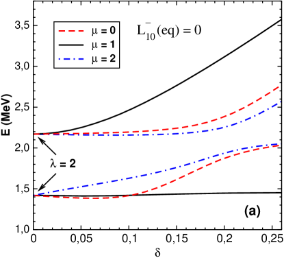
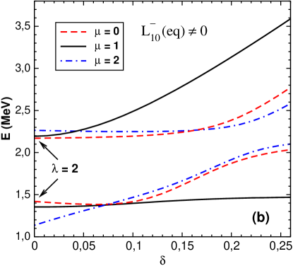
Figure 1: Energies $E$ of the low-lying $\mu=0,1,2$ levels as a function of deformation $\delta$. (a) The calculations were performed without $L^{-}_{10}$(eq). (b) Splitting of the $2^{+}$ states into three branches in a spherical nucleus as a result of accounting for nuclear antiferromagnetism: $L^{-}_{10}({\rm eq})=L^{{{\uparrow\uparrow}}}_{10}({\rm eq})-L^{{{\downarrow\downarrow}}}_{10}({\rm eq})$.

First of all, we note that this state is not a spurious mode. The WFM method ensures the conservation of the total angular momentum BaMo ; BaMoPRC13 (see Appendix C) and, as a result, does not produce the spurious state. In the absence of coupling, the lowest level with an energy of 1.29 MeV is an isoscalar state of an irrotational nature with large $B(E2)$ value and near to zero $B(M1)$ strength. The isoscalar-isovector coupling strongly affects this state, reducing its $B(E2)$ value by almost half (from 43 W.u. up to 25 W.u.). However, it retains its electrical nature, and its energy changes only from 1.29 MeV to 1.47 MeV (see Table 1).

The nature of this state can be understood after solving dynamical equations for irreducible tensors (9) with $\mu=2$ and $\mu=0$ (see Appendix A), and studying the deformation dependence of the found low-lying levels. The results of required calculations for ¹⁶⁴Dy are shown in Fig. 1(a). They demonstrate in an obvious way that the lowest $1.47$ MeV $1^{+}$ state is just one of three ($K^{\pi}=0^{+},1^{+},2^{+}$) branches of $J^{\pi}=2^{+}$ state, which can exist in a spherical nucleus (and which splits due to deformation into three branches with projections $\mu=0,\pm 1,\pm 2$).

In a spherical nucleus the equations for different $\lambda$ are decoupled. The equations describing the dynamics of $\lambda=2$ variables, in addition to the state that is the subject of our interest, give one more low-lying solution, which is a quadrupole vibrational “ground” of the orbital scissors (see Fig. 1(a)). As shown in BaMoPRC22 , the scissors mode is a mixture of rotational and irrotational flows (see also section IV Currents). In a spherical nucleus, rotational oscillations are not excited Balb22 . However, due to the coupled dynamics of the conventional scissors mode and isovector GQR BaSc ; Ann , the vibrational $2^{+}$ state is excited at the energy of 2.17 MeV with a small value of $B(E2)=0.63$ W.u.. As can be seen from the Fig. 1(a), in the deformed nucleus this level also splits into three branches with different $K^{\pi}$.

It is necessary to say that there is one more item that must be taken into account in the calculations. The point is that the results used to draw Fig. 1(a) are approximate ones. They are obtained by neglecting the equilibrium value of the collective variable $L^{\tau-}_{10}$(eq), which is responsible for the phenomenon of “hidden angular momenta” BaMoPRC2 . By definition, $L^{\tau-}_{10}=L^{\tau{{\uparrow\uparrow}}}_{10}-L^{\tau{{\downarrow\downarrow}}}_{10}$, where $L^{\tau{{\uparrow\uparrow}}}_{10}$ and $L^{\tau{{\downarrow\downarrow}}}_{10}$ are the average values of the $z$-component of the orbital angular momentum of all nucleons with the spin projections $\uparrow$ and $\downarrow$ respectively. It was shown in BaMoPRC2 , that $L^{\tau{{\uparrow\uparrow}}}_{10}\mbox{\rm(eq)}=-L^{\tau{{\downarrow\downarrow}}}_{10}$(eq) in the equilibrium state. So, the ground-state nucleus consists of two equal parts having nonzero angular momenta with opposite directions, which compensate each other resulting in the zero total angular momentum ($L^{\tau+}_{10}\mbox{\rm(eq)}=L^{\tau{{\uparrow\uparrow}}}_{10}\mbox{\rm(eq)}+L^{\tau{{\downarrow\downarrow}}}_{10}\mbox{\rm(eq)}=0$), whereas $L^{\tau-}_{10}\mbox{\rm(eq)}\neq 0$ even in the spherical limit. This phenomenon is quite similar to the phenomenon of the antiferromagnetism Gurevich , so we will use in the following namely this term.

The simplest model of an antiferromagnet is one in which it is represented as a set of two equivalent interpenetrating magnetic sublattices characterized by the same value but antiparallel oriented magnetization densities Akhiezer . In the ground state, the magnetic moments of the sublattices are compensated. The action of an external magnetic field leads to the appearance of a macroscopic magnetic moment of the antiferromagnet. The manifestation of antiferromagnetism in our calculations is a consequence of the fact that the WFM method deals with a dynamic mean field BaMoPRC13 ; Balb22 . The resulting splitting is the reaction of the mean field of the nucleus to an external perturbation. The results of calculations, including $L^{\tau-}_{10}$(eq)), are shown in Fig. 1(b). It is seen that taking into account the antiferromagnetic properties of nuclei leads to the splitting of $2^{+}$ states already at zero deformation. It is interesting to note that the energy of the lowest $\mu=1$ state weakly depends on the deformation (see Figs. 1(a), 1(b)), while the $E2$ strength decreases from $25.44$ W.u. to $15.56$ W.u. in the spherical limit.

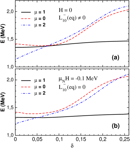
Figure 2: The $\mu=0,1,2$ energy branches of nucleus with $N$ and $Z$ corresponding to ¹⁶⁴Dy vs. deformation $\delta$. The results of calculations with $L_{10}^{-}\neq 0,{\cal H}=0$ (a) and $L_{10}^{-}=0,{\cal H}\neq 0$ (b) (see also columns I and III in Table 2).

To verify the relevance of the analogy with antiferromagnetism, we compare the effect of $L^{\tau-}_{10}$(eq) with the influence of an external magnetic field Gurevich ; Davydov . In the absence of an external magnetic field the states with different projections of the nuclear magnetic moment onto the quantization axis are degenerate. When an external magnetic field ${\cal H}$ is applied, the magnetic moment acquires the potential energy in this field (Zeeman energy) and, as a result, the degeneracy of states with different projections is removed. According to Davydov , the action of a uniform magnetic field ${\cal H}$ can be described in a linear approximation by adding to the Hamiltonian the term ${\cal M}=-\hat{\mu}\cdot\hat{{\cal H}}$, where

$$\hat{\mu}=\frac{e}{2mc}\sum\limits_{\tau={\rm p,n}}\left(g_{l}^{\tau}\hat{\bf l}^{\tau}+g_{s}^{\tau}\hat{\bf s}^{\tau}\right)$$ (10)

is the operator of the magnetic moment of the nucleus, $\hat{\bf l}=[\hat{{\bf r}}\times\hat{{\bf p}}]$ – the orbital angular momentum, $\hat{{\bf p}}=-i\hbar\bf{\nabla}$, $\hat{\bf s}=\frac{\hbar}{2}\hat{\bf\sigma}$ – the spin operator, $\hat{\sigma}$ – Pauli matrix, $g_{l}$ and $g_{s}$ are orbital and spin $g$-factors (see Appendix B).

Table 2: The calculated splitting of $2^{+}$ state which can exist in spherical nucleus with N and Z corresponding to ¹⁶⁴Dy:
I – $L_{10}^{-}({\rm eq})=22i\hbar$, ${\cal H}=0$,
II – $L_{10}^{-}({\rm eq})=0$, $\mu_{N}{\cal H}=-0.13$ MeV,
III – $L_{10}^{-}({\rm eq})=0$, $\mu_{N}{\cal H}=-0.1$ MeV,
IV – $L_{10}^{-}({\rm eq})=0$, $\mu_{N}{\cal H}=-0.05$ MeV.

$\mu$	$E$, MeV
	I	II	III	IV
0	1.42	1.42	1.42	1.42
1	1.35	1.28	1.32	1.37
2	1.14	1.15	1.21	1.31

Let us consider the magnetic field directed along $z$-axis. In this case $\hat{{\cal H}}={\cal H}_{z}\equiv{\cal H}$ and

$${\cal M}^{\tau} =-\frac{e{\cal H}}{2mc}(g_{l}^{\tau}\hat{l_{0}}+g_{s}^{\tau}\hat{s_{0}})$$

$$=\frac{e\hbar{\cal H}}{2mc}\left(g_{l}^{\tau}\sqrt{2}\{\hat{r}\otimes\nabla\}_{10}-\frac{g_{s}^{\tau}}{2}\hat{\sigma_{0}}\right).$$

The Wigner transformation of ${\cal M}^{\tau}$ reads:

$${\cal M}^{\tau}_{W}=\frac{e{\cal H}}{2mc}\left(g_{l}^{\tau}i\sqrt{2}\{r\otimes p\}_{10}-g_{s}^{\tau}\frac{\hbar}{2}{\sigma_{0}}\right).$$

By definition $h^{\pm}=h^{\uparrow\uparrow}\pm h^{\downarrow\downarrow}$. Remembering that $\sigma_{0}={1\quad\,0\choose\,0\;\;\;-\!1}$ Var , one finds

$$h_{W}^{\tau+}=i\mu_{N}{\cal H}g_{l}^{\tau}\frac{2\sqrt{2}}{\hbar}\{r\otimes p\}_{10},\quad h_{W}^{\tau-}=-g_{s}^{\tau}\,\mu_{N}{\cal H},$$

where $\mu_{N}=\frac{e\hbar}{2mc}$ is the nuclear magneton. The contribution of the magnetic field into dynamical equations for variables ${\cal L}^{\tau\varsigma}_{\lambda\mu}(t)$, ${\cal R}^{\tau\varsigma}_{\lambda\mu}(t)$, ${\cal P}^{\tau\varsigma}_{\lambda\mu}(t)$ is written out in Appendix A. There are 24 equations for $\mu=2$, 44 equations for $\mu=1$ and 52 ones for $\mu=0$. It is worth to note, that magnetic field contributes into all 24 equations for $\mu=2$, into 38 equations for $\mu=1$ and into 16 equations for $\mu=0$, whereas $L_{10}^{-}$(eq) enters only in two equations for $\mu=1$ and $\mu=2$, and does not contribute to the equations for $\mu=0$. Nevertheless their influence on the splitting of $2^{+}$ state turns out quite close (at the proper choice of the magnetic field strength ${\cal H}$). At the zero deformation, the energy of splitting (Zeeman energy) is $\Delta E\simeq\mu{\cal H}\mu_{N}$ MeV. The results of calculations with $L_{10}^{-}\neq 0,{\cal H}=0$ and $L_{10}^{-}=0,{\cal H}\neq 0$ for the lowest state are compared in the Table 2 and Fig. 2 (a, b). There are no fundamental differences between the effect produced by nuclear antiferromagnetism and the result obtained when a uniform magnetic field is turned on. Remarkably, the nuclear level spacing $\sim 0.1$ MeV gives respective field strength scale ${\cal H}=\Delta E/\mu_{N}\sim$ 1 TT (Teratesla) = $10^{16}$ G (Gauss), which is comparable to the range of magnetic strength of magnetars Pena .

What variables are responsible for the generation of this excitation? First of all, it is the branch of the splitted 2⁺ state, which can exist in spherical nuclei. Therefore, the respective variables should have $\lambda=2$. Furthermore, the calculations without pair correlations show, that the energy of this state goes to zero if to omit the variables ${\cal R}^{\uparrow\downarrow}_{22}$, ${\cal R}^{\downarrow\uparrow}_{20}$, ${\cal P}^{\uparrow\downarrow}_{22}$, ${\cal P}^{\downarrow\uparrow}_{20}$ together with their dynamical equations (see Appendix A). According to the spin indexes, these variables describe spin-flip processes. Similarly, the solution disappears if variables ${\cal R}^{+}_{21}$ and ${\cal P}^{+}_{21}$ are omitted together with their dynamical equations. The natural conclusion is that these two sets of variables are the generators of the excitation. This fact allows one to suppose the rather interesting peculiarity of the excitation process of this nuclear mode: the electric external field $\hat{O}_{21}=er^{2}Y_{21}$ (see Appendix B) initiates the dynamical deformation ${\cal R}^{+}_{21}(t)$ together with the Fermi surface deformation ${\cal P}^{+}_{21}(t)$, which in their turn initiate spin-flip transitions ${\cal R}^{\uparrow\downarrow}_{22}(t)$, ${\cal R}^{\downarrow\uparrow}_{20}(t)$, ${\cal P}^{\uparrow\downarrow}_{22}(t)$, ${\cal P}^{\downarrow\uparrow}_{20}(t)$. Our calculations show that this is the only low-lying state in the formation of which spin-flip variables are involved.

IV Currents

The analysis of currents of three low-lying magnetic excitations had shown that every of them represents rather complicate mixture of all three possible scissors modes BaMoPRC22 . Besides, as Lipparini and Stringari LS83 and later Balbutsev et al Malov ; Ann have shown, microscopically there is a strong coupling between the scissors mode and the isovector GQR. Actually without this coupling the scissors mode comes at zero energy. The result of this coupling is also that the rotation is accompanied by a quadrupole distortion of the shape of the nucleus, see BaSc .

Now it will be interesting to analyze the structure of currents corresponding to the electric excitation disposed at the energy $E=1.47$ MeV, just below all scissors modes. The detailed description of the procedure of constructing nuclear currents is given in the paper BaMoPRC22 .

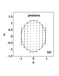
Figure 3: The proton and neutron currents in ¹⁶⁴Dy for the lowest electrical level with energy $E=1.29$ MeV. The calculations were performed without the isoscalar-isovector coupling. Here and below, a sharp-edge density distribution is used for visualization; y $=y/R_{0}$, z $=z/R_{0}$, $R_{0}$ – nuclear radius.

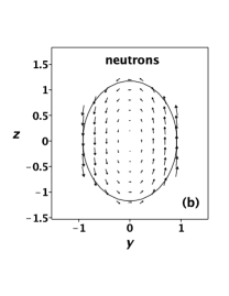
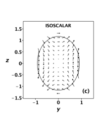
Figure 4: The currents in ¹⁶⁴Dy for the lowest electrical level with energy $E=1.47$ MeV. The isoscalar-isovector coupling is taken into account.

The resulting spin-scalar current field can be represented as a superposition of rotational and vibrational fields

$${\bf J}^{\tau}({\bf r})=n({\bf r})\left[a^{\tau}\left[{\bf e}_{x}\times{\bf r}\right]+b^{\tau}\nabla(yz)\right],$$ (11)

with amplitudes $a^{\tau}$ and $b^{\tau}$ respectively

$$a^{\tau}=3i\,\frac{{\cal L}^{+\tau}_{11}\left(1+\delta/3\right)+\delta{\cal L}^{+\tau}_{21}}{Q_{00}\left(1-2/3\delta\right)\left(1+4/3\delta\right)},$$

$$b^{\tau}=3i\,\frac{{\cal L}^{+\tau}_{21}\left(1+\delta/3\right)+\delta{\cal L}^{+\tau}_{11}}{Q_{00}\left(1-2/3\delta\right)\left(1+4/3\delta\right)},$$ (12)

where $n({\bf r})$ – nuclear density distribution, $\delta$ – deformation (see Appendix A for parameters). As can be seen from (11, IV), the rotational contribution is determined predominantly by the $\mu=1$ projection of the collective orbital angular momentum ${\cal L}^{+\tau}_{11}$, while the vibrational component is determined mainly by the value of the variable ${\cal L}^{+\tau}_{21}$ which represents the velocity of changing of the nuclear shape (${\cal L}^{+\tau}_{21}\sim\dot{{\cal R}}^{+\tau}_{21}$). It was shown in BaMoPRC22 that in the case of three magnetic excitations the field (11) is flat, all motions take place only in one plane, as it should be for real scissors. The same is true for the considered excitation.

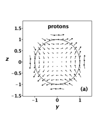
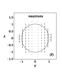
Figure 5: The currents in the nucleus with $N$ and $Z$ corresponding to ¹⁶⁴Dy for the lowest electrical level: (a),(b) – $\delta=0$, (c),(d) – $\delta=0.02$, (e),(f) – $\delta=0.032$, (g),(h) – $\delta=0.06$.

Calculations performed without the coupling of isovector and isoscalar equations demonstrate a clear quadrupole vibrational pattern (see Fig. 3, where the currents of neutrons and protons are shown separately). Protons and neutrons move in phase. This is the expected result, since in such approximation the considered solution is purely isoscalar (see Table 1). Taking into account the isovector-isoscalar coupling greatly changes the pattern of flows. As can be seen from Fig. 4 (a, b), both currents acquire a rotational character. The trajectories of nucleons are the strongly stretched (prolate) ellipses, their long axes being perpendicular one to another. The overall picture is close to a shear displacements. The sum of proton and neutron currents is shown in Fig. 4 (c). Surprisingly, the character of the displacements turns out almost pure vibrational. This result is confirmed by the rather large $B(E2)$ value (see Table 1, first line). The isovector contribution is shown in Fig. 4 (d). It is almost purely rotational, that obviously corresponds to the conventional scissors (see Table 1, fourth line).

Let us stress, that we define the isoscalar (isovector) mode as the sum (difference) of neutron and proton amplitudes, independently of the character of their relative motion – in phase or out of phase. For example, it is impossible to say anything definite about the relative phase of neutron and proton currents in Figs. 4 (a) and 4 (b). Nevertheless their sum and difference (Figs. 4 (c) and 4 (d)) produce evident pictures of the isoscalar vibrational and the isovector rotational motions.

Finally, it is interesting to investigate the behavior of currents in the spherical limit ($\delta=0$). The collective rotation is completely absent at zero deformation. So in this case, as expected, we obtain an undoubtedly quadrupole vibrational picture for considered constituents, which is shown in the Fig. 5 (a, b). As a consequence, this leads to an increase in the value of $B(E2)$ up to 43 W.u. and $B(M1)=0$ $\mu_{N}^{2}$. But even negligibly small deviation from a spherical shape immediately transforms the vibrational motion of protons and neutrons into the “shear-rotational” one. The evolution of the flow distributions with increasing deformation is tracked down in Fig. 5 (a, b, c, d, e, f, g, h). Such behavior is a direct effect of the isoscalar-isovector coupling, which enables the admixture of the scissors rotation. Thus, the analysis shows that in even-even heavy nuclei, the collective motion of protons and neutrons associated with low-energy quadrupole vibrational excitations is strongly influenced by the scissors-like rotation. Although the summed flow distribution of nucleons retains its vibrational character, the isovector contribution has an appreciable effect.

We are only considering convection currents here. As discussed in the previous section, spin-flip processes are essential for the formation of the state under consideration. In the future, we plan to study the effect of spin currents. It is also important to note that if the spin degrees of freedom are neglected, this solution goes to zero BaMo .

The present analysis shows that the electrical state considered here has a complex internal structure, but invariably demonstrates an overall irrotational flow pattern.

V Conclusion

The WFM method was applied to solve TDHFB equations for the harmonic oscillator with the spin-orbital potential plus quadrupole-quadrupole and spin-spin residual interactions. The dynamics of collective variables ${\cal L}^{\tau\varsigma}_{\lambda\mu}(t)$, ${\cal R}^{\tau\varsigma}_{\lambda\mu}(t)$ and ${\cal P}^{\tau\varsigma}_{\lambda\mu}(t)$ with $\lambda=1,2$ and $\mu=0,1,2$ was studied taking into account pair correlations.

The subject of the especial interest was the predicted low-lying $K^{\pi}=1^{+}$ excitation located at 1.47 MeV, below of all scissors modes, and having a $B(E2)$ value of 25.44 W.u., which allowed us to assume the electric character of this state. It is found that this state is one of three branches of $2^{+}$ state which can exist in spherical nuclei and which is split due to the deformation. An analysis of the dynamical equations allows us to conclude that the variables describing the quadrupole distortions of the shape of the nucleus ${\cal R}^{+}_{21}(t)$, the Fermi surface deformation ${\cal P}^{+}_{21}(t)$, as well as the variables ${\cal R}^{\uparrow\downarrow}_{22}(t)$, ${\cal R}^{\downarrow\uparrow}_{20}(t)$, ${\cal P}^{\uparrow\downarrow}_{22}(t)$, ${\cal P}^{\downarrow\uparrow}_{20}(t)$ associated with spin-flip processes, are predominantly responsible for the formation of this excitation. The underlying physical nature of this mode is revealed by an examination of the nucleons currents. Despite the complex internal structure of the flow, which is determined by the superposition of irrotational and rotational contributions, the nucleus as a whole demonstrates the quadrupole character of collective oscillations. All this confirms the conclusion about the electrical nature of the state under study.

It is discovered, that the antiferromagnetic properties of nuclei lead to the splitting of the low-lying $2^{+}$ states already at the zero deformation. Nuclear antiferromagnetism is expressed in the nonzero equilibrium value of the variable $L^{\tau-}_{10}$ and manifests itself as a response of the dynamic mean field to an external perturbation. It is shown that splitting of $2+$ states in spherical nuclei induced by the nuclear antiferromagnetism is very similar to the Zeeman splitting in an external uniform magnetic field.

Appendix A Dynamical equations

The set of dynamical equations for isovector variables with $\mu=2$ reads

$$\dot{\bar{\cal L}}^{+}_{22} = 2\frac{i}{\hbar}\mu_{N}{\cal H}\bar{\cal L}^{+}_{22}+\frac{1}{m}\bar{\cal P}^{+}_{22}-m\,\omega^{2}\bar{\cal R}^{+}_{22}-i\hbar\eta\left[\bar{\cal L}^{-}_{22}+\bar{\cal L}^{{\downarrow\uparrow}}_{21}\right]$$

$$+2\kappa_{0}\left[\left(\left(1+\alpha\right)Q_{20}-2\alpha Q_{00}\right)\bar{\cal R}^{+}_{22}+\left(\left(1+\alpha\right)\bar{Q}_{20}-2\bar{Q}_{00}\right){\cal R}^{+}_{22}\right],$$

$$\dot{\bar{\cal R}}^{+}_{22} = 2\frac{i}{\hbar}\mu_{N}{\cal H}\bar{\cal R}^{+}_{22}+\frac{2}{m}\bar{\cal L}^{+}_{22}-i\hbar\eta\left[\bar{\cal R}^{-}_{22}+\bar{\cal R}^{{\downarrow\uparrow}}_{21}\right],$$

$$\dot{\bar{\cal P}}^{+}_{22} = 2\frac{i}{\hbar}\mu_{N}{\cal H}\bar{\cal P}^{+}_{22}-2m\,\omega^{2}\bar{\cal L}^{+}_{22}+4\kappa_{0}\left[Q_{20}\bar{\cal L}^{+}_{22}+\alpha\bar{Q}_{20}{\cal L}^{+}_{22}\right]-i\hbar\eta\left[\bar{\cal P}^{-}_{22}+\bar{\cal P}^{{\downarrow\uparrow}}_{21}\right]$$

$$+\frac{3I_{2}\hbar^{2}}{2A_{1}A_{2}}\chi\left[\left({Q_{00}}+{Q_{20}}\right)\bar{\cal L}^{+}_{22}+\left({\bar{Q}_{00}}+{\bar{Q}_{20}}\right){\cal L}^{+}_{22}\right]+\frac{4}{\hbar}\left[I_{pp}^{\kappa\Delta}{\bar{\tilde{\cal P}}}_{22}+\bar{I}_{pp}^{\kappa\Delta}{\tilde{\cal P}}_{22}\right],$$

$$\dot{\bar{\cal L}}^{-}_{22} = 2\frac{i}{\hbar}\mu_{N}{\cal H}\bar{\cal L}^{-}_{22}+\frac{1}{m}\bar{\cal P}^{-}_{22}-m\,\omega^{2}\bar{\cal R}^{-}_{22}+2\kappa_{0}\left[Q_{20}\bar{\cal R}^{-}_{22}+\alpha\bar{Q}_{20}{\cal R}^{-}_{22}\right]-i\hbar\eta\bar{\cal L}^{+}_{22}$$

$$+\frac{I_{1}\hbar^{2}}{15A_{1}A_{2}}\left[\left(3\chi-\bar{\chi}\right)\left({Q_{00}}+{Q_{20}}\right)\bar{\cal R}^{-}_{22}+\left(3\chi+\bar{\chi}\right)\left({\bar{Q}_{00}}+{\bar{Q}_{20}}\right){\cal R}^{-}_{22}\right]+\frac{4}{\hbar}\left[I_{rp}^{\kappa\Delta}{\bar{\tilde{\cal L}}}_{22}+\bar{I}_{rp}^{\kappa\Delta}{{\tilde{\cal L}}}_{22}\right],$$

$$\dot{\bar{\cal R}}^{-}_{22} = 2\frac{i}{\hbar}\mu_{N}{\cal H}\bar{\cal R}^{-}_{22}+\frac{2}{m}\bar{\cal L}^{-}_{22}-i\hbar\eta\bar{\cal R}^{+}_{22},$$

$$\dot{\bar{\cal P}}^{-}_{22} = 2\frac{i}{\hbar}\mu_{N}{\cal H}\bar{\cal P}^{-}_{22}-2m\,\omega^{2}\bar{\cal L}^{-}_{22}+4\kappa_{0}\left[Q_{20}\bar{\cal L}^{-}_{22}+\alpha\bar{Q}_{20}{\cal L}^{-}_{22}\right]-12\sqrt{2}\kappa_{0}\left[\alpha L^{-}_{10}({\rm eq})\bar{\cal R}^{+}_{22}+\bar{L}^{-}_{10}({\rm eq}){\cal R}^{+}_{22}\right]$$

$$-i\hbar\eta\bar{\cal P}^{+}_{22}+\frac{3I_{2}\hbar^{2}}{2A_{1}A_{2}}\chi\left[\left({Q_{00}}+{Q_{20}}\right)\bar{\cal L}^{-}_{22}+\left({\bar{Q}_{00}}+{\bar{Q}_{20}}\right){\cal L}^{-}_{22}\right],$$

$$\dot{\bar{\cal L}}^{{{\downarrow\uparrow}}}_{21} = \frac{i}{\hbar}\mu_{N}{\cal H}(2-g)\bar{\cal L}^{{\downarrow\uparrow}}_{21}+\frac{1}{m}\bar{\cal P}^{{\downarrow\uparrow}}_{21}-\left[m\,\omega^{2}+\kappa_{0}Q_{20}\right]\bar{\cal R}^{{\downarrow\uparrow}}_{21}-\alpha\kappa_{0}\bar{Q}_{20}{\cal R}^{{\downarrow\uparrow}}_{21}-i\hbar\frac{\eta}{2}\bar{\cal L}^{+}_{22}$$

$$+\frac{I_{1}\hbar^{2}}{15A_{1}A_{2}}\left[\left(3\chi-\bar{\chi}\right)\left({Q_{00}}+{Q_{20}}/4\right)\bar{\cal R}^{{\downarrow\uparrow}}_{21}+\left(3\chi+\bar{\chi}\right)\left({\bar{Q}_{00}}+{\bar{Q}_{20}}/4\right){\cal R}^{{\downarrow\uparrow}}_{21}\right],$$

$$\dot{\bar{\cal R}}^{{\downarrow\uparrow}}_{21} = \frac{i}{\hbar}\mu_{N}{\cal H}(2-g)\bar{\cal R}^{{\downarrow\uparrow}}_{21}+\frac{2}{m}\bar{\cal L}^{{\downarrow\uparrow}}_{21}-i\hbar\frac{\eta}{2}\bar{\cal R}^{+}_{22},$$

$$\dot{\bar{\cal P}}^{{{\downarrow\uparrow}}}_{21} = \frac{i}{\hbar}\mu_{N}{\cal H}(2-g)\bar{\cal P}^{{\downarrow\uparrow}}_{21}-2m\,\omega^{2}\bar{\cal L}^{{\downarrow\uparrow}}_{21}+2\kappa_{0}\left[Q_{20}\left(3\bar{\cal L}^{{\downarrow\uparrow}}_{11}-\bar{\cal L}^{{\downarrow\uparrow}}_{21}\right)+\alpha\bar{Q}_{20}\left(3{\cal L}^{{\downarrow\uparrow}}_{11}-{\cal L}^{{\downarrow\uparrow}}_{21}\right)\right]-i\hbar\frac{\eta}{2}\bar{\cal P}^{+}_{22}$$

$$+\frac{3I_{2}\hbar^{2}}{8A_{1}A_{2}}\chi\left[3{Q_{20}}\bar{\cal L}^{{\downarrow\uparrow}}_{11}+\left(4{Q_{00}}+{Q_{20}}\right)\bar{\cal L}^{{\downarrow\uparrow}}_{21}+3{\bar{Q}_{20}}{\cal L}^{{\downarrow\uparrow}}_{11}+\left(4{\bar{Q}_{00}}+{\bar{Q}_{20}}\right){\cal L}^{{\downarrow\uparrow}}_{21}\right],$$

$$\dot{\bar{\cal L}}^{{{\downarrow\uparrow}}}_{11} = \frac{i}{\hbar}\mu_{N}{\cal H}(2-g)\bar{\cal L}^{{\downarrow\uparrow}}_{11}-3\kappa_{0}\left[Q_{20}\bar{\cal R}^{{\downarrow\uparrow}}_{21}+\alpha\bar{Q}_{20}{\cal R}^{{\downarrow\uparrow}}_{21}\right]-\frac{I_{1}\hbar^{2}}{20A_{1}A_{2}}\left[\left(3\chi-\bar{\chi}\right){Q_{20}}\bar{\cal R}^{{\downarrow\uparrow}}_{21}+\left(3\chi+\bar{\chi}\right){\bar{Q}_{20}}{\cal R}^{{\downarrow\uparrow}}_{21}\right],$$

$$\dot{\bar{\tilde{\cal L}}}_{22} = 2\frac{i}{\hbar}\mu_{N}{\cal H}{\bar{\tilde{\cal L}}}_{22}-\frac{\Delta}{2\hbar}\bar{\cal L}^{-}_{22}-\frac{\bar{\Delta}}{2\hbar}{\cal L}^{-}_{22},$$

$$\dot{\bar{\tilde{\cal P}}}_{22} = 2\frac{i}{\hbar}\mu_{N}{\cal H}{\bar{\tilde{\cal P}}}_{22}-\frac{\Delta}{2\hbar}\bar{\cal P}^{+}_{22}-\frac{\bar{\Delta}}{2\hbar}{\cal P}^{+}_{22}+3\hbar\kappa_{0}\left[\alpha K_{0}\bar{\cal R}^{+}_{22}+\bar{K}_{0}{\cal R}^{+}_{22}\right].$$ (13)

The set of dynamical equations for isoscalar variables with $\mu=2$ reads

$$\dot{{\cal L}}^{+}_{22} = -2\frac{i}{\hbar}\mu_{N}{\cal H}{\cal L}^{+}_{22}+\frac{1}{m}{\cal P}^{+}_{22}-m\,\omega^{2}{\cal R}^{+}_{22}-i\hbar\eta\left[{\cal L}^{-}_{22}+{\cal L}^{{\downarrow\uparrow}}_{21}\right]$$

$$+4\kappa_{0}\left[\left(Q_{20}-Q_{00}\right){\cal R}^{+}_{22}+\alpha\left(\bar{Q}_{20}-\bar{Q}_{00}\right)\bar{\cal R}^{+}_{22}\right],$$

$$\dot{{\cal R}}^{+}_{22} = -2\frac{i}{\hbar}\mu_{N}{\cal H}{\cal R}^{+}_{22}+\frac{2}{m}{\cal L}^{+}_{22}-i\hbar\eta\left[{\cal R}^{-}_{22}+{\cal R}^{{\downarrow\uparrow}}_{21}\right],$$

$$\dot{{\cal P}}^{+}_{22} = -2\frac{i}{\hbar}\mu_{N}{\cal H}{\cal P}^{+}_{22}-2m\,\omega^{2}{\cal L}^{+}_{22}+4\kappa_{0}\left[Q_{20}{\cal L}^{+}_{22}+\alpha\bar{Q}_{20}\bar{\cal L}^{+}_{22}\right]-i\hbar\eta\left[{\cal P}^{-}_{22}+{\cal P}^{{\downarrow\uparrow}}_{21}\right]$$

$$+\frac{3I_{2}\hbar^{2}}{2A_{1}A_{2}}\chi\left[\left({Q_{00}}+{Q_{20}}\right)\bar{\cal L}^{+}_{22}+\left({\bar{Q}_{00}}+{\bar{Q}_{20}}\right){\cal L}^{+}_{22}\right]+\frac{4}{\hbar}\left[I_{pp}^{\kappa\Delta}{{\tilde{\cal P}}}_{22}+\bar{I}_{pp}^{\kappa\Delta}{\bar{\tilde{\cal P}}}_{22}\right],$$

$$\dot{{\cal L}}^{-}_{22} = -2\frac{i}{\hbar}\mu_{N}{\cal H}{\cal L}^{-}_{22}+\frac{1}{m}{\cal P}^{-}_{22}-m\,\omega^{2}{\cal R}^{-}_{22}+2\kappa_{0}\left[Q_{20}{\cal R}^{-}_{22}+\alpha\bar{Q}_{20}\bar{\cal R}^{-}_{22}\right]+\frac{4}{\hbar}\left[I_{rp}^{\kappa\Delta}{{\tilde{\cal L}}}_{22}+\bar{I}_{rp}^{\kappa\Delta}{\bar{\tilde{\cal L}}}_{22}\right]$$

$$-i\hbar\eta{\cal L}^{+}_{22}+\frac{I_{1}\hbar^{2}}{15A_{1}A_{2}}\left[\left(3\chi+\bar{\chi}\right)\left({Q_{00}}+{Q_{20}}\right){\cal R}^{-}_{22}+\left(3\chi-\bar{\chi}\right)\left({\bar{Q}_{00}}+{\bar{Q}_{20}}\right)\bar{\cal R}^{-}_{22}\right],$$

$$\dot{{\cal R}}^{-}_{22} = -2\frac{i}{\hbar}\mu_{N}{\cal H}{\cal R}^{-}_{22}+\frac{2}{m}{\cal L}^{-}_{22}-i\hbar\eta{\cal R}^{+}_{22},$$

$$\dot{{\cal P}}^{-}_{22} = -2\frac{i}{\hbar}\mu_{N}{\cal H}{\cal P}^{-}_{22}-2m\,\omega^{2}{\cal L}^{-}_{22}+4\kappa_{0}\left[Q_{20}{\cal L}^{-}_{22}+\alpha\bar{Q}_{20}\bar{\cal L}^{-}_{22}\right]-12\sqrt{2}\kappa_{0}\left[L^{-}_{10}({\rm eq}){\cal R}^{+}_{22}+\alpha\bar{L}^{-}_{10}({\rm eq})\bar{\cal R}^{+}_{22}\right]$$

$$-i\hbar\eta{\cal P}^{+}_{22}+\frac{3I_{2}\hbar^{2}}{2A_{1}A_{2}}\chi\left[\left({Q_{00}}+{Q_{20}}\right){\cal L}^{-}_{22}+\left({\bar{Q}_{00}}+{\bar{Q}_{20}}\right)\bar{\cal L}^{-}_{22}\right],$$

$$\dot{{\cal L}}^{{{\downarrow\uparrow}}}_{21} = -\frac{i}{\hbar}\mu_{N}{\cal H}(2+g){\cal L}^{{\downarrow\uparrow}}_{21}+\frac{1}{m}{\cal P}^{{\downarrow\uparrow}}_{21}-\left[m\,\omega^{2}+\kappa_{0}Q_{20}\right]{\cal R}^{{\downarrow\uparrow}}_{21}-\alpha\kappa_{0}\bar{Q}_{20}\bar{\cal R}^{{\downarrow\uparrow}}_{21}-i\hbar\frac{\eta}{2}{\cal L}^{+}_{22}$$

$$+\frac{I_{1}\hbar^{2}}{15A_{1}A_{2}}\left[\left(3\chi+\bar{\chi}\right)\left({Q_{00}}+{Q_{20}}/4\right){\cal R}^{{\downarrow\uparrow}}_{21}+\left(3\chi-\bar{\chi}\right)\left({\bar{Q}_{00}}+{\bar{Q}_{20}}/4\right)\bar{\cal R}^{{\downarrow\uparrow}}_{21}\right],$$

$$\dot{{\cal R}}^{{\downarrow\uparrow}}_{21} = -\frac{i}{\hbar}\mu_{N}{\cal H}(2+g){\cal R}^{{\downarrow\uparrow}}_{21}+\frac{2}{m}{\cal L}^{{\downarrow\uparrow}}_{21}-i\hbar\frac{\eta}{2}{\cal R}^{+}_{22},$$

$$\dot{{\cal P}}^{{{\downarrow\uparrow}}}_{21} = -\frac{i}{\hbar}\mu_{N}{\cal H}(2+g){\cal P}^{{\downarrow\uparrow}}_{21}-2m\,\omega^{2}{\cal L}^{{\downarrow\uparrow}}_{21}+2\kappa_{0}\left[Q_{20}\left(3{\cal L}^{{\downarrow\uparrow}}_{11}-{\cal L}^{{\downarrow\uparrow}}_{21}\right)+\alpha\bar{Q}_{20}\left(3\bar{\cal L}^{{\downarrow\uparrow}}_{11}-\bar{\cal L}^{{\downarrow\uparrow}}_{21}\right)\right]-i\hbar\frac{\eta}{2}{\cal P}^{+}_{22}$$

$$+\frac{3I_{2}\hbar^{2}}{8A_{1}A_{2}}\chi\left[3{Q_{20}}{\cal L}^{{\downarrow\uparrow}}_{11}+\left(4{Q_{00}}+{Q_{20}}\right){\cal L}^{{\downarrow\uparrow}}_{21}+3{\bar{Q}_{20}}\bar{\cal L}^{{\downarrow\uparrow}}_{11}+\left(4{\bar{Q}_{00}}+{\bar{Q}_{20}}\right)\bar{\cal L}^{{\downarrow\uparrow}}_{21}\right],$$

$$\dot{{\cal L}}^{{{\downarrow\uparrow}}}_{11} = -\frac{i}{\hbar}\mu_{N}{\cal H}(2+g){\cal L}^{{\downarrow\uparrow}}_{11}-3\kappa_{0}\left[Q_{20}{\cal R}^{{\downarrow\uparrow}}_{21}+\alpha\bar{Q}_{20}\bar{\cal R}^{{\downarrow\uparrow}}_{21}\right]-\frac{I_{1}\hbar^{2}}{20A_{1}A_{2}}\left[\left(3\chi+\bar{\chi}\right){Q_{20}}{\cal R}^{{\downarrow\uparrow}}_{21}+\left(3\chi-\bar{\chi}\right){\bar{Q}_{20}}\bar{\cal R}^{{\downarrow\uparrow}}_{21}\right],$$

$$\dot{{\tilde{\cal L}}}_{22} = -2\frac{i}{\hbar}\mu_{N}{\cal H}{{\tilde{\cal L}}}_{22}-\frac{\Delta}{2\hbar}{\cal L}^{-}_{22}-\frac{\bar{\Delta}}{2\hbar}\bar{\cal L}^{-}_{22},$$

$$\dot{{\tilde{\cal P}}}_{22} = -2\frac{i}{\hbar}\mu_{N}{\cal H}{{\tilde{\cal P}}}_{22}-\frac{\Delta}{2\hbar}{\cal P}^{+}_{22}-\frac{\bar{\Delta}}{2\hbar}\bar{\cal P}^{+}_{22}+3\hbar\kappa_{0}\left[K_{0}{\cal R}^{+}_{22}+\alpha\bar{K}_{0}\bar{\cal R}^{+}_{22}\right].$$ (14)

The set of dynamical equations for isovector variables with $\mu=1$ reads

$$\dot{\bar{\cal L}}^{+}_{21} = \frac{i}{\hbar}\mu_{N}{\cal H}\bar{\cal L}^{+}_{21}+\frac{1}{m}\bar{\cal P}_{21}^{+}-\left[m\,\omega^{2}+\kappa_{0}\left(4\alpha Q_{00}+(1+\alpha)Q_{20}\right)\right]\bar{\cal R}^{+}_{21}-i\hbar\frac{\eta}{2}\left[\bar{\cal L}_{21}^{-}+2\bar{\cal L}^{{\uparrow\downarrow}}_{22}+\sqrt{6}\bar{\cal L}^{{\downarrow\uparrow}}_{20}\right]$$

$$-\kappa_{0}\left(4\bar{Q}_{00}+(1+\alpha)\bar{Q}_{20}\right){\cal R}^{+}_{21},$$

$$\dot{\bar{\cal L}}^{-}_{21} = \frac{i}{\hbar}\mu_{N}{\cal H}\bar{\cal L}^{-}_{21}+\frac{1}{m}\bar{\cal P}_{21}^{-}-\left[m\,\omega^{2}+\kappa_{0}Q_{20}-\frac{\hbar^{2}}{15}\left(3\chi-\bar{\chi}\right)\frac{I_{1}}{A_{1}A_{2}}\left(Q_{00}+Q_{20}/4\right)\right]\bar{\cal R}^{-}_{21}-i\hbar\frac{\eta}{2}\bar{\cal L}_{21}^{+}$$

$$+\frac{4}{\hbar}I_{rp}^{\kappa\Delta}(r^{\prime}){\bar{\tilde{\cal L}}}_{21}-\left[\alpha\kappa_{0}\bar{Q}_{20}-\frac{\hbar^{2}}{15}\left(3\chi+\bar{\chi}\right)\frac{I_{1}}{A_{1}A_{2}}\left(\bar{Q}_{00}+\bar{Q}_{20}/4\right)\right]{\cal R}^{-}_{21}+\frac{4}{\hbar}\bar{I}_{rp}^{\kappa\Delta}(r^{\prime}){{\tilde{\cal L}}}_{21},$$

$$\dot{\bar{\cal L}}^{{\uparrow\downarrow}}_{22} = \frac{1}{m}\bar{\cal P}_{22}^{{\uparrow\downarrow}}-\left[m\,\omega^{2}-2\kappa_{0}Q_{20}-\frac{\hbar^{2}}{15}\left(3\chi-\bar{\chi}\right)\frac{\sqrt{3}I_{1}}{A_{2}}\right]\bar{\cal R}^{{\uparrow\downarrow}}_{22}-i\hbar\frac{\eta}{2}\bar{\cal L}_{21}^{+}$$

$$+\left[2\alpha\kappa_{0}\bar{Q}_{20}+\frac{\hbar^{2}}{15}\left(3\chi+\bar{\chi}\right)\frac{I_{1}}{A_{1}A_{2}}\left(\bar{Q}_{20}+\bar{Q}_{00}\right)\right]{\cal R}^{{\uparrow\downarrow}}_{22},$$

$$\dot{\bar{\cal L}}^{{\downarrow\uparrow}}_{20} = \frac{i}{\hbar}\mu_{N}{\cal H}(1-g)\bar{\cal L}^{{\downarrow\uparrow}}_{20}+\frac{1}{m}\bar{\cal P}_{20}^{{\downarrow\uparrow}}-\left[m\,\omega^{2}+2\kappa_{0}Q_{20}\right]\bar{\cal R}^{{\downarrow\uparrow}}_{20}+2\sqrt{2}\kappa_{0}Q_{20}\,\bar{\cal R}^{{\downarrow\uparrow}}_{00}-i\hbar\frac{\eta}{2}\sqrt{\frac{3}{2}}\bar{\cal L}_{21}^{+}$$

$$+\frac{\hbar^{2}}{15}\left(3\chi-\bar{\chi}\right)\frac{I_{1}}{A_{1}A_{2}}\,\left[Q_{00}\bar{\cal R}_{20}^{{\downarrow\uparrow}}+Q_{20}\bar{\cal R}_{00}^{{\downarrow\uparrow}}/\sqrt{2}\right],$$

$$-2\alpha\kappa_{0}\bar{Q}_{20}\left[{\cal R}_{20}^{{\downarrow\uparrow}}+\sqrt{2}{\cal R}_{00}^{{\downarrow\uparrow}}\right]+\frac{\hbar^{2}}{15}\left(3\chi+\bar{\chi}\right)\frac{I_{1}}{A_{1}A_{2}}\,\left[\bar{Q}_{00}{\cal R}_{20}^{{\downarrow\uparrow}}+\bar{Q}_{20}{\cal R}_{00}^{{\downarrow\uparrow}}/\sqrt{2}\right],$$

$$\dot{\bar{\cal L}}^{+}_{11} = \frac{i}{\hbar}\mu_{N}{\cal H}\bar{\cal L}^{+}_{11}-3(1-\alpha)\kappa_{0}Q_{20}\,\bar{\cal R}^{+}_{21}-i\hbar\frac{\eta}{2}\left[\bar{\cal L}_{11}^{-}+\sqrt{2}\bar{\cal L}^{{\downarrow\uparrow}}_{10}\right]+3(1-\alpha)\kappa_{0}\bar{Q}_{20}\,{\cal R}^{+}_{21},$$

$$\dot{\bar{\cal L}}^{-}_{11} = \frac{i}{\hbar}\mu_{N}{\cal H}\bar{\cal L}^{-}_{11}-\left[3\kappa_{0}Q_{20}+\frac{\hbar^{2}}{20}\left(3\chi-\bar{\chi}\right)\frac{I_{1}}{A_{1}A_{2}}Q_{20}\right]\bar{\cal R}^{-}_{21}+\frac{4}{\hbar}I_{rp}^{\kappa\Delta}(r^{\prime}){\bar{\tilde{\cal L}}}_{11}-\hbar\frac{\eta}{2}\left[i\bar{\cal L}_{11}^{+}+\hbar\bar{\cal F}^{{\downarrow\uparrow}}\right]$$

$$-\left[3\alpha\kappa_{0}\bar{Q}_{20}+\frac{\hbar^{2}}{20}\left(3\chi+\bar{\chi}\right)\frac{I_{1}}{A_{1}A_{2}}\bar{Q}_{20}\right]{\cal R}^{-}_{21}+\frac{4}{\hbar}\bar{I}_{rp}^{\kappa\Delta}(r^{\prime}){{\tilde{\cal L}}}_{11},$$

$$\dot{\bar{\cal L}}^{{\downarrow\uparrow}}_{10} = \frac{i}{\hbar}\mu_{N}{\cal H}(1-g)\bar{\cal L}^{{\downarrow\uparrow}}_{10}-\hbar\frac{\eta}{2\sqrt{2}}\left[i\bar{\cal L}_{11}^{+}+\hbar\bar{\cal F}^{{\downarrow\uparrow}}\right],$$

$$\dot{\bar{\cal F}}^{{\downarrow\uparrow}} = \frac{i}{\hbar}\mu_{N}{\cal H}(1-g)\bar{\cal F}^{{\downarrow\uparrow}}-\eta\left[\bar{\cal L}_{11}^{-}+\sqrt{2}\bar{\cal L}^{{\downarrow\uparrow}}_{10}\right],$$

$$\dot{\bar{\cal R}}^{+}_{21} = \frac{i}{\hbar}\mu_{N}{\cal H}\bar{\cal R}^{+}_{21}+\frac{2}{m}\bar{\cal L}_{21}^{+}-i\hbar\frac{\eta}{2}\left[\bar{\cal R}_{21}^{-}+2\bar{\cal R}^{{\uparrow\downarrow}}_{22}+\sqrt{6}\bar{\cal R}^{{\downarrow\uparrow}}_{20}\right],$$

$$\dot{\bar{\cal R}}^{-}_{21} = \frac{i}{\hbar}\mu_{N}{\cal H}\bar{\cal R}^{-}_{21}+\frac{2}{m}\bar{\cal L}_{21}^{-}-i\hbar\frac{\eta}{2}\bar{\cal R}_{21}^{+},$$

$$\dot{\bar{\cal R}}^{{\uparrow\downarrow}}_{22} = \frac{2}{m}\bar{\cal L}_{22}^{{\uparrow\downarrow}}-i\hbar\frac{\eta}{2}\bar{\cal R}_{21}^{+},$$

$$\dot{\bar{\cal R}}^{{\downarrow\uparrow}}_{20} = \frac{i}{\hbar}\mu_{N}{\cal H}(1-g)\bar{\cal R}^{{\downarrow\uparrow}}_{20}+\frac{2}{m}\bar{\cal L}_{20}^{{\downarrow\uparrow}}-i\hbar\frac{\eta}{2}\sqrt{\frac{3}{2}}\bar{\cal R}_{21}^{+},$$

$$\dot{\bar{\cal P}}^{+}_{21} = \frac{i}{\hbar}\mu_{N}{\cal H}\bar{\cal P}^{+}_{21}-2\left[m\,\omega^{2}+\kappa_{0}Q_{20}\right]\bar{\cal L}^{+}_{21}+6\kappa_{0}Q_{20}\bar{\cal L}^{+}_{11}-i\hbar\frac{\eta}{2}\left[\bar{\cal P}_{21}^{-}+2\bar{\cal P}^{{\uparrow\downarrow}}_{22}+\sqrt{6}\bar{\cal P}^{{\downarrow\uparrow}}_{20}\right]$$

$$+\frac{3}{8}\hbar^{2}\chi\frac{I_{2}}{A_{1}A_{2}}\left[\left(Q_{20}+4Q_{00}\right)\bar{\cal L}_{21}^{+}+3Q_{20}\bar{\cal L}_{11}^{+}\right]+\frac{4}{\hbar}I_{pp}^{\kappa\Delta}(r^{\prime}){\bar{\tilde{\cal P}}}_{21}$$

$$+2\alpha\kappa_{0}\bar{Q}_{20}\left(3{\cal L}^{+}_{11}-{\cal L}^{+}_{21}\right)+\frac{3}{8}\hbar^{2}\chi\frac{I_{2}}{A_{1}A_{2}}\left[\left(\bar{Q}_{20}+4\bar{Q}_{00}\right){\cal L}_{21}^{+}+3\bar{Q}_{20}{\cal L}_{11}^{+}\right]+\frac{4}{\hbar}\bar{I}_{pp}^{\kappa\Delta}(r^{\prime}){{\tilde{\cal P}}}_{21},$$

$$\dot{\bar{\cal P}}^{-}_{21} = \frac{i}{\hbar}\mu_{N}{\cal H}\bar{\cal P}^{-}_{21}-2\left[m\,\omega^{2}+\kappa_{0}Q_{20}\right]\bar{\cal L}^{-}_{21}+6\kappa_{0}Q_{20}\bar{\cal L}^{-}_{11}-6\sqrt{2}\alpha\kappa_{0}L_{10}^{-}({\rm eq})\bar{\cal R}^{+}_{21}-i\hbar\frac{\eta}{2}\bar{\cal P}_{21}^{+}$$

$$+\frac{3}{8}\hbar^{2}\chi\frac{I_{2}}{A_{1}A_{2}}\left[\left(Q_{20}+4Q_{00}\right)\bar{\cal L}_{21}^{-}+3Q_{20}\bar{\cal L}_{11}^{-}\right]+2\alpha\kappa_{0}\bar{Q}_{20}\left(3{\cal L}^{-}_{11}-{\cal L}^{-}_{21}\right)$$

$$+\frac{3}{8}\hbar^{2}\chi\frac{I_{2}}{A_{1}A_{2}}\left[\left(\bar{Q}_{20}+4\bar{Q}_{00}\right){\cal L}_{21}^{-}+3\bar{Q}_{20}{\cal L}_{11}^{-}\right]-6\sqrt{2}\kappa_{0}\bar{L}_{10}^{-}({\rm eq}){\cal R}^{+}_{21},$$

$$\dot{\bar{\cal P}}^{{\uparrow\downarrow}}_{22} = -2\left[m\,\omega^{2}-2\kappa_{0}Q_{20}\right]\bar{\cal L}^{{\uparrow\downarrow}}_{22}-i\hbar\frac{\eta}{2}\bar{\cal P}_{21}^{+}+\frac{3}{2}\hbar^{2}\chi\frac{I_{2}}{A_{1}A_{2}}\left(Q_{20}+Q_{00}\right)\bar{\cal L}^{{\uparrow\downarrow}}_{22}$$

$$+4\alpha\kappa_{0}\bar{Q}_{20}{\cal L}^{{\uparrow\downarrow}}_{22}+\frac{3}{2}\hbar^{2}\chi\frac{I_{2}}{A_{1}A_{2}}\left(\bar{Q}_{20}+\bar{Q}_{00}\right){\cal L}^{{\uparrow\downarrow}}_{22},$$

$$\dot{\bar{\cal P}}^{{\downarrow\uparrow}}_{20} = \frac{i}{\hbar}\mu_{N}{\cal H}(1-g)\bar{\cal P}^{{\downarrow\uparrow}}_{20}-2\left[m\,\omega^{2}+2\kappa_{0}Q_{20}\right]\bar{\cal L}^{{\downarrow\uparrow}}_{20}+4\sqrt{2}\kappa_{0}Q_{20}\bar{\cal L}^{{\downarrow\uparrow}}_{00}-i\hbar\frac{\eta}{2}\sqrt{\frac{3}{2}}\bar{\cal P}_{21}^{+}$$

$$+\frac{3}{2}\hbar^{2}\chi\frac{I_{2}}{A_{1}A_{2}}\left[Q_{00}\bar{\cal L}_{20}^{{\downarrow\uparrow}}+Q_{20}\bar{\cal L}_{00}^{{\downarrow\uparrow}}/\sqrt{2}\right]+4\alpha\kappa_{0}\bar{Q}_{20}\left(\sqrt{2}{\cal L}^{{\downarrow\uparrow}}_{00}-{\cal L}^{{\downarrow\uparrow}}_{20}\right)$$

$$+\frac{3}{2}\hbar^{2}\chi\frac{I_{2}}{A_{1}A_{2}}\left[\bar{Q}_{00}{\cal L}_{20}^{{\downarrow\uparrow}}+\bar{Q}_{20}{\cal L}_{00}^{{\downarrow\uparrow}}/\sqrt{2}\right],$$

$$\dot{\bar{\cal L}}^{{\downarrow\uparrow}}_{00} = \frac{i}{\hbar}\mu_{N}{\cal H}(1-g)\bar{\cal L}^{{\downarrow\uparrow}}_{00}+\frac{1}{m}\bar{\cal P}_{00}^{{\downarrow\uparrow}}-m\,\omega^{2}\bar{\cal R}^{{\downarrow\uparrow}}_{00}+2\sqrt{2}\kappa_{0}Q_{20}\bar{\cal R}^{{\downarrow\uparrow}}_{20}$$

$$+\frac{\hbar^{2}}{4\,A_{1}A_{2}}\left[\left(\chi-\frac{\bar{\chi}}{3}\right)I_{1}-\frac{9}{4}\chi I_{2}\right]\left[\left(2Q_{00}+Q_{20}\right)\bar{\cal R}_{00}^{{\downarrow\uparrow}}+\sqrt{2}Q_{20}\bar{\cal R}_{20}^{{\downarrow\uparrow}}\right]$$

$$+2\sqrt{2}\alpha\kappa_{0}\bar{Q}_{20}{\cal R}^{{\downarrow\uparrow}}_{20}+\frac{\hbar^{2}}{4\,A_{1}A_{2}}\left[\left(\chi+\frac{\bar{\chi}}{3}\right)I_{1}-\frac{9}{4}\chi I_{2}\right]\left[\left(2\bar{Q}_{00}+\bar{Q}_{20}\right){\cal R}_{00}^{{\downarrow\uparrow}}+\sqrt{2}\bar{Q}_{20}{\cal R}_{20}^{{\downarrow\uparrow}}\right],$$

$$\dot{\bar{\cal R}}^{{\downarrow\uparrow}}_{00} = \frac{i}{\hbar}\mu_{N}{\cal H}(1-g)\bar{\cal R}^{{\downarrow\uparrow}}_{00}+\frac{2}{m}\bar{\cal L}_{00}^{{\downarrow\uparrow}},$$

$$\dot{\bar{\cal P}}^{{\downarrow\uparrow}}_{00} = \frac{i}{\hbar}\mu_{N}{\cal H}(1-g)\bar{\cal P}^{{\downarrow\uparrow}}_{00}+-2m\,\omega^{2}\bar{\cal L}^{{\downarrow\uparrow}}_{00}+4\sqrt{2}\kappa_{0}Q_{20}\bar{\cal L}^{{\downarrow\uparrow}}_{20}+\frac{3}{4}\hbar^{2}\chi\frac{I_{2}}{A_{1}A_{2}}\left[\left(2Q_{00}+Q_{20}\right)\bar{\cal L}_{00}^{{\downarrow\uparrow}}+\sqrt{2}Q_{20}\bar{\cal L}_{20}^{{\downarrow\uparrow}}\right]$$

$$+4\sqrt{2}\alpha\kappa_{0}\bar{Q}_{20}{\cal L}^{{\downarrow\uparrow}}_{20}+\frac{3}{4}\hbar^{2}\chi\frac{I_{2}}{A_{1}A_{2}}\left[\left(2\bar{Q}_{00}+\bar{Q}_{20}\right){\cal L}_{00}^{{\downarrow\uparrow}}+\sqrt{2}\bar{Q}_{20}{\cal L}_{20}^{{\downarrow\uparrow}}\right],$$

$$\dot{\bar{\tilde{\cal P}}}_{21} = \frac{i}{\hbar}\mu_{N}{\cal H}{\bar{\tilde{\cal P}}}_{21}-\frac{1}{2\hbar}\Delta(r^{\prime})\bar{\cal P}^{+}_{21}+6\hbar\alpha\kappa_{0}K_{0}{\bar{\cal R}}^{+}_{21}-\frac{1}{2\hbar}\bar{\Delta}(r^{\prime}){\cal P}^{+}_{21}+6\hbar\kappa_{0}\bar{K}_{0}{{\cal R}}^{+}_{21},$$

$$\dot{\bar{\tilde{\cal L}}}_{21} = \frac{i}{\hbar}\mu_{N}{\cal H}{\bar{\tilde{\cal L}}}_{21}-\frac{1}{2\hbar}\Delta(r^{\prime})\bar{\cal L}^{-}_{21}-\frac{1}{2\hbar}\bar{\Delta}(r^{\prime}){\cal L}^{-}_{21},$$

$$\dot{\bar{\tilde{\cal L}}}_{11} = \frac{i}{\hbar}\mu_{N}{\cal H}{\bar{\tilde{\cal L}}}_{11}-\frac{1}{2\hbar}\Delta(r^{\prime})\bar{\cal L}^{-}_{11}-\frac{1}{2\hbar}\bar{\Delta}(r^{\prime}){\cal L}^{-}_{11}.$$ (15)

The set of dynamical equations for isoscalar variables with $\mu=1$ reads

$$\dot{{\cal L}}^{+}_{21} = -\frac{i}{\hbar}\mu_{N}{\cal H}{\cal L}^{+}_{21}+\frac{1}{m}{\cal P}_{21}^{+}-\left[m\,\omega^{2}+2\kappa_{0}\left(2Q_{00}+Q_{20}\right)\right]{\cal R}^{+}_{21}-i\hbar\frac{\eta}{2}\left[{\cal L}_{21}^{-}+2{\cal L}^{{\uparrow\downarrow}}_{22}+\sqrt{6}{\cal L}^{{\downarrow\uparrow}}_{20}\right]$$

$$-\alpha\kappa_{0}\left(2\bar{Q}_{00}+\bar{Q}_{20}\right)\bar{\cal R}^{+}_{21},$$

$$\dot{{\cal L}}^{-}_{21} = -\frac{i}{\hbar}\mu_{N}{\cal H}{\cal L}^{-}_{21}+\frac{1}{m}{\cal P}_{21}^{-}-\left[m\,\omega^{2}+\kappa_{0}Q_{20}-\frac{\hbar^{2}}{15}\left(3\chi+\bar{\chi}\right)\frac{I_{1}}{A_{1}A_{2}}\left(Q_{00}+Q_{20}/4\right)\right]{\cal R}^{-}_{21}-i\hbar\frac{\eta}{2}{\cal L}_{21}^{+}$$

$$+\frac{4}{\hbar}I_{rp}^{\kappa\Delta}(r^{\prime}){{\tilde{\cal L}}}_{21}-\left[\alpha\kappa_{0}\bar{Q}_{20}-\frac{\hbar^{2}}{15}\left(3\chi-\bar{\chi}\right)\frac{I_{1}}{A_{1}A_{2}}\left(\bar{Q}_{00}+\bar{Q}_{20}/4\right)\right]\bar{\cal R}^{-}_{21}+\frac{4}{\hbar}\bar{I}_{rp}^{\kappa\Delta}(r^{\prime}){\bar{\tilde{\cal L}}}_{21},$$

$$\dot{{\cal L}}^{{\uparrow\downarrow}}_{22} = \frac{1}{m}{\cal P}_{22}^{{\uparrow\downarrow}}-\left[m\,\omega^{2}-2\kappa_{0}Q_{20}-\frac{\hbar^{2}}{15}\left(3\chi+\bar{\chi}\right)\frac{\sqrt{3}I_{1}}{A_{2}}\right]{\cal R}^{{\uparrow\downarrow}}_{22}-i\hbar\frac{\eta}{2}{\cal L}_{21}^{+}$$

$$+\left[2\alpha\kappa_{0}\bar{Q}_{20}+\frac{\hbar^{2}}{15}\left(3\chi-\bar{\chi}\right)\frac{I_{1}}{A_{1}A_{2}}\left(\bar{Q}_{20}+\bar{Q}_{00}\right)\right]\bar{\cal R}^{{\uparrow\downarrow}}_{22},$$

$$\dot{{\cal L}}^{{\downarrow\uparrow}}_{20} = -\frac{i}{\hbar}\mu_{N}{\cal H}(1+g){\cal L}^{{\downarrow\uparrow}}_{20}+\frac{1}{m}{\cal P}_{20}^{{\downarrow\uparrow}}-\left[m\,\omega^{2}+2\kappa_{0}Q_{20}\right]{\cal R}^{{\downarrow\uparrow}}_{20}+2\sqrt{2}\kappa_{0}Q_{20}\,{\cal R}^{{\downarrow\uparrow}}_{00}-i\hbar\frac{\eta}{2}\sqrt{\frac{3}{2}}{\cal L}_{21}^{+}$$

$$+\frac{\hbar^{2}}{15}\left(3\chi+\bar{\chi}\right)\frac{I_{1}}{A_{1}A_{2}}\,\left[Q_{00}{\cal R}_{20}^{{\downarrow\uparrow}}+Q_{20}{\cal R}_{00}^{{\downarrow\uparrow}}/\sqrt{2}\right],$$

$$-2\alpha\kappa_{0}\bar{Q}_{20}\left[\bar{\cal R}_{20}^{{\downarrow\uparrow}}+\sqrt{2}\bar{\cal R}_{00}^{{\downarrow\uparrow}}\right]+\frac{\hbar^{2}}{15}\left(3\chi-\bar{\chi}\right)\frac{I_{1}}{A_{1}A_{2}}\,\left[\bar{Q}_{00}\bar{\cal R}_{20}^{{\downarrow\uparrow}}+\bar{Q}_{20}\bar{\cal R}_{00}^{{\downarrow\uparrow}}/\sqrt{2}\right],$$

$$\dot{{\cal L}}^{+}_{11} = -\frac{i}{\hbar}\mu_{N}{\cal H}{\cal L}^{+}_{11}-i\hbar\frac{\eta}{2}\left[{\cal L}_{11}^{-}+\sqrt{2}{\cal L}^{{\downarrow\uparrow}}_{10}\right],$$

$$\dot{{\cal L}}^{-}_{11} = -\frac{i}{\hbar}\mu_{N}{\cal H}{\cal L}^{-}_{11}-\left[3\kappa_{0}Q_{20}+\frac{\hbar^{2}}{20}\left(3\chi+\bar{\chi}\right)\frac{I_{1}}{A_{1}A_{2}}Q_{20}\right]{\cal R}^{-}_{21}+\frac{4}{\hbar}I_{rp}^{\kappa\Delta}(r^{\prime}){{\tilde{\cal L}}}_{11}-\hbar\frac{\eta}{2}\left[i{\cal L}_{11}^{+}+\hbar{\cal F}^{{\downarrow\uparrow}}\right]$$

$$-\left[3\alpha\kappa_{0}\bar{Q}_{20}+\frac{\hbar^{2}}{20}\left(3\chi-\bar{\chi}\right)\frac{I_{1}}{A_{1}A_{2}}\bar{Q}_{20}\right]\bar{\cal R}^{-}_{21}+\frac{4}{\hbar}\bar{I}_{rp}^{\kappa\Delta}(r^{\prime}){\bar{\tilde{\cal L}}}_{11},$$

$$\dot{{\cal L}}^{{\downarrow\uparrow}}_{10} = -\frac{i}{\hbar}\mu_{N}{\cal H}(1+g){\cal L}^{{\downarrow\uparrow}}_{10}-\hbar\frac{\eta}{2\sqrt{2}}\left[i{\cal L}_{11}^{+}+\hbar{\cal F}^{{\downarrow\uparrow}}\right],$$

$$\dot{{\cal F}}^{{\downarrow\uparrow}} = -\frac{i}{\hbar}\mu_{N}{\cal H}(1+g){\cal F}^{{\downarrow\uparrow}}-\eta\left[{\cal L}_{11}^{-}+\sqrt{2}{\cal L}^{{\downarrow\uparrow}}_{10}\right],$$

$$\dot{{\cal R}}^{+}_{21} = -\frac{i}{\hbar}\mu_{N}{\cal H}{\cal R}^{+}_{21}\frac{2}{m}{\cal L}_{21}^{+}-i\hbar\frac{\eta}{2}\left[{\cal R}_{21}^{-}+2{\cal R}^{{\uparrow\downarrow}}_{22}+\sqrt{6}{\cal R}^{{\downarrow\uparrow}}_{20}\right],$$

$$\dot{{\cal R}}^{-}_{21} = -\frac{i}{\hbar}\mu_{N}{\cal H}{\cal R}^{-}_{21}\frac{2}{m}{\cal L}_{21}^{-}-i\hbar\frac{\eta}{2}{\cal R}_{21}^{+},$$

$$\dot{{\cal R}}^{{\uparrow\downarrow}}_{22} = \frac{2}{m}{\cal L}_{22}^{{\uparrow\downarrow}}-i\hbar\frac{\eta}{2}{\cal R}_{21}^{+},$$

$$\dot{{\cal R}}^{{\downarrow\uparrow}}_{20} = -\frac{i}{\hbar}\mu_{N}{\cal H}(1+g){\cal R}^{{\downarrow\uparrow}}_{20}+\frac{2}{m}{\cal L}_{20}^{{\downarrow\uparrow}}-i\hbar\frac{\eta}{2}\sqrt{\frac{3}{2}}{\cal R}_{21}^{+},$$

$$\dot{{\cal P}}^{+}_{21} = -\frac{i}{\hbar}\mu_{N}{\cal H}{\cal P}^{+}_{21}-2\left[m\,\omega^{2}+\kappa_{0}Q_{20}\right]{\cal L}^{+}_{21}+6\kappa_{0}Q_{20}{\cal L}^{+}_{11}-i\hbar\frac{\eta}{2}\left[{\cal P}_{21}^{-}+2{\cal P}^{{\uparrow\downarrow}}_{22}+\sqrt{6}{\cal P}^{{\downarrow\uparrow}}_{20}\right]$$

$$+\frac{3}{8}\hbar^{2}\chi\frac{I_{2}}{A_{1}A_{2}}\left[\left(Q_{20}+4Q_{00}\right){\cal L}_{21}^{+}+3Q_{20}{\cal L}_{11}^{+}\right]+\frac{4}{\hbar}I_{pp}^{\kappa\Delta}(r^{\prime}){{\tilde{\cal P}}}_{21}$$

$$+2\alpha\kappa_{0}\bar{Q}_{20}\left(3\bar{\cal L}^{+}_{11}-\bar{\cal L}^{+}_{21}\right)+\frac{3}{8}\hbar^{2}\chi\frac{I_{2}}{A_{1}A_{2}}\left[\left(\bar{Q}_{20}+4\bar{Q}_{00}\right)\bar{\cal L}_{21}^{+}+3\bar{Q}_{20}\bar{\cal L}_{11}^{+}\right]+\frac{4}{\hbar}\bar{I}_{pp}^{\kappa\Delta}(r^{\prime}){\bar{\tilde{\cal P}}}_{21},$$

$$\dot{{\cal P}}^{-}_{21} = -\frac{i}{\hbar}\mu_{N}{\cal H}{\cal P}^{-}_{21}-2\left[m\,\omega^{2}+\kappa_{0}Q_{20}\right]{\cal L}^{-}_{21}+6\kappa_{0}Q_{20}{\cal L}^{-}_{11}-6\sqrt{2}\kappa_{0}L_{10}^{-}({\rm eq}){\cal R}^{+}_{21}-i\hbar\frac{\eta}{2}{\cal P}_{21}^{+}$$

$$+\frac{3}{8}\hbar^{2}\chi\frac{I_{2}}{A_{1}A_{2}}\left[\left(Q_{20}+4Q_{00}\right){\cal L}_{21}^{-}+3Q_{20}{\cal L}_{11}^{-}\right]$$

$$+2\alpha\kappa_{0}\bar{Q}_{20}\left(3\bar{\cal L}^{-}_{11}-\bar{\cal L}^{-}_{21}\right)+\frac{3}{8}\hbar^{2}\chi\frac{I_{2}}{A_{1}A_{2}}\left[\left(\bar{Q}_{20}+4\bar{Q}_{00}\right)\bar{\cal L}_{21}^{-}+3\bar{Q}_{20}\bar{\cal L}_{11}^{-}\right]-6\sqrt{2}\alpha\kappa_{0}\bar{L}_{10}^{-}({\rm eq})\bar{\cal R}^{+}_{21},$$

$$\dot{{\cal P}}^{{\uparrow\downarrow}}_{22} = -2\left[m\,\omega^{2}-2\kappa_{0}Q_{20}\right]{\cal L}^{{\uparrow\downarrow}}_{22}-i\hbar\frac{\eta}{2}{\cal P}_{21}^{+}+\frac{3}{2}\hbar^{2}\chi\frac{I_{2}}{A_{1}A_{2}}\left(Q_{20}+Q_{00}\right){\cal L}^{{\uparrow\downarrow}}_{22}$$

$$+4\alpha\kappa_{0}\bar{Q}_{20}\bar{\cal L}^{{\uparrow\downarrow}}_{22}+\frac{3}{2}\hbar^{2}\chi\frac{I_{2}}{A_{1}A_{2}}\left(\bar{Q}_{20}+\bar{Q}_{00}\right)\bar{\cal L}^{{\uparrow\downarrow}}_{22},$$

$$\dot{{\cal P}}^{{\downarrow\uparrow}}_{20} = -\frac{i}{\hbar}\mu_{N}{\cal H}(1+g){\cal P}^{{\downarrow\uparrow}}_{20}-2\left[m\,\omega^{2}+2\kappa_{0}Q_{20}\right]{\cal L}^{{\downarrow\uparrow}}_{20}+4\sqrt{2}\kappa_{0}Q_{20}{\cal L}^{{\downarrow\uparrow}}_{00}-i\hbar\frac{\eta}{2}\sqrt{\frac{3}{2}}{\cal P}_{21}^{+}$$

$$+\frac{3}{2}\hbar^{2}\chi\frac{I_{2}}{A_{1}A_{2}}\left[Q_{00}{\cal L}_{20}^{{\downarrow\uparrow}}+Q_{20}{\cal L}_{00}^{{\downarrow\uparrow}}/\sqrt{2}\right]+4\alpha\kappa_{0}\bar{Q}_{20}\left(\sqrt{2}\bar{\cal L}^{{\downarrow\uparrow}}_{00}-\bar{\cal L}^{{\downarrow\uparrow}}_{20}\right)$$

$$+\frac{3}{2}\hbar^{2}\chi\frac{I_{2}}{A_{1}A_{2}}\left[\bar{Q}_{00}{\cal L}_{20}^{{\downarrow\uparrow}}+\bar{Q}_{20}\bar{\cal L}_{00}^{{\downarrow\uparrow}}/\sqrt{2}\right],$$

$$\dot{{\cal L}}^{{\downarrow\uparrow}}_{00} = -\frac{i}{\hbar}\mu_{N}{\cal H}(1+g){\cal L}^{{\downarrow\uparrow}}_{00}+\frac{1}{m}{\cal P}_{00}^{{\downarrow\uparrow}}-m\,\omega^{2}{\cal R}^{{\downarrow\uparrow}}_{00}+2\sqrt{2}\kappa_{0}Q_{20}{\cal R}^{{\downarrow\uparrow}}_{20}$$

$$+\frac{\hbar^{2}}{4\,A_{1}A_{2}}\left[\left(\chi+\frac{\bar{\chi}}{3}\right)I_{1}-\frac{9}{4}\chi I_{2}\right]\left[\left(2Q_{00}+Q_{20}\right){\cal R}_{00}^{{\downarrow\uparrow}}+\sqrt{2}Q_{20}{\cal R}_{20}^{{\downarrow\uparrow}}\right]$$

$$+2\sqrt{2}\alpha\kappa_{0}\bar{Q}_{20}\bar{\cal R}^{{\downarrow\uparrow}}_{20}+\frac{\hbar^{2}}{4\,A_{1}A_{2}}\left[\left(\chi-\frac{\bar{\chi}}{3}\right)I_{1}-\frac{9}{4}\chi I_{2}\right]\left[\left(2\bar{Q}_{00}+\bar{Q}_{20}\right)\bar{\cal R}_{00}^{{\downarrow\uparrow}}+\sqrt{2}\bar{Q}_{20}\bar{\cal R}_{20}^{{\downarrow\uparrow}}\right],$$

$$\dot{{\cal R}}^{{\downarrow\uparrow}}_{00} = -\frac{i}{\hbar}\mu_{N}{\cal H}(1+g){\cal R}^{{\downarrow\uparrow}}_{00}+\frac{2}{m}{\cal L}_{00}^{{\downarrow\uparrow}},$$

$$\dot{{\cal P}}^{{\downarrow\uparrow}}_{00} = -\frac{i}{\hbar}\mu_{N}{\cal H}(1+g){\cal P}^{{\downarrow\uparrow}}_{00}-2m\,\omega^{2}{\cal L}^{{\downarrow\uparrow}}_{00}+4\sqrt{2}\kappa_{0}Q_{20}{\cal L}^{{\downarrow\uparrow}}_{20}+\frac{3}{4}\hbar^{2}\chi\frac{I_{2}}{A_{1}A_{2}}\left[\left(2Q_{00}+Q_{20}\right)\bar{\cal L}_{00}^{{\downarrow\uparrow}}+\sqrt{2}Q_{20}\bar{\cal L}_{20}^{{\downarrow\uparrow}}\right]$$

$$+4\sqrt{2}\alpha\kappa_{0}\bar{Q}_{20}\bar{\cal L}^{{\downarrow\uparrow}}_{20}+\frac{3}{4}\hbar^{2}\chi\frac{I_{2}}{A_{1}A_{2}}\left[\left(2\bar{Q}_{00}+\bar{Q}_{20}\right)\bar{\cal L}_{00}^{{\downarrow\uparrow}}+\sqrt{2}\bar{Q}_{20}\bar{\cal L}_{20}^{{\downarrow\uparrow}}\right],$$

$$\dot{{\tilde{\cal P}}}_{21} = -\frac{i}{\hbar}\mu_{N}{\cal H}\tilde{\cal P}_{21}-\frac{1}{2\hbar}\Delta(r^{\prime}){\cal P}^{+}_{21}+6\hbar\kappa_{0}K_{0}{\cal R}^{+}_{21}-\frac{1}{2\hbar}\bar{\Delta}(r^{\prime})\bar{\cal P}^{+}_{21}+6\hbar\alpha\kappa_{0}\bar{K}_{0}\bar{\cal R}^{+}_{21},$$

$$\dot{{\tilde{\cal L}}}_{21} = -\frac{i}{\hbar}\mu_{N}{\cal H}\tilde{\cal L}_{21}-\frac{1}{2\hbar}\Delta(r^{\prime}){\cal L}^{-}_{21}-\frac{1}{2\hbar}\bar{\Delta}(r^{\prime})\bar{\cal L}^{-}_{21},$$

$$\dot{{\tilde{\cal L}}}_{11} = -\frac{i}{\hbar}\mu_{N}{\cal H}\tilde{\cal L}_{11}-\frac{1}{2\hbar}\Delta(r^{\prime}){\cal L}^{-}_{11}-\frac{1}{2\hbar}\bar{\Delta}(r^{\prime})\bar{\cal L}^{-}_{11}.$$ (16)

The set of dynamical equations for isovector variables with $\mu=0$ reads

$$\dot{\bar{\cal L}}^{+}_{20} = \frac{1}{m}{\cal P}^{+}_{20}-\left[m\,\omega^{2}+2\kappa_{0}\left((1+\alpha){Q_{20}}+2\alpha{Q_{00}}\right)\right]\bar{\cal R}^{+}_{20}+2\sqrt{2}\kappa_{0}{Q_{20}}\bar{\cal R}^{+}_{00}-i\hbar\frac{\eta}{2}\sqrt{6}\left[\bar{\cal L}^{{\uparrow\downarrow}}_{21}+\bar{\cal L}^{{\downarrow\uparrow}}_{2-1}\right]$$

$$-2\kappa_{0}\left[\left((1+\alpha){\bar{Q}_{20}}+2{\bar{Q}_{00}}\right){\cal R}^{+}_{20}-\sqrt{2}\alpha{\bar{Q}_{20}}{\cal R}^{+}_{00}\right],$$

$$\dot{\bar{\cal R}}^{+}_{20} = \frac{2}{m}\bar{\cal L}^{+}_{20}-i\hbar\frac{\eta}{2}\sqrt{6}\left[{\cal R}^{{\uparrow\downarrow}}_{21}+{\cal R}^{{\downarrow\uparrow}}_{2-1}\right],$$

$$\dot{\bar{\cal P}}^{+}_{20} = -2\left[m\,\omega^{2}+2\kappa_{0}{Q_{20}}\right]\bar{\cal L}^{+}_{20}+4\sqrt{2}\kappa_{0}{Q_{20}}\bar{\cal L}^{+}_{00}-4\alpha\kappa_{0}{\bar{Q}_{20}}\left[{\cal L}^{+}_{20}-\sqrt{2}{\cal L}^{+}_{00}\right]$$

$$-i\hbar\frac{\eta}{2}\sqrt{6}\left[\bar{\cal P}^{{\uparrow\downarrow}}_{21}+\bar{\cal P}^{{\downarrow\uparrow}}_{2-1}\right]+\frac{4}{\hbar}\left[I_{pp}^{\kappa\Delta}{\bar{\tilde{\cal P}}}_{20}+\bar{I}_{pp}^{\kappa\Delta}{{\tilde{\cal P}}}_{20}\right]$$

$$+\frac{3I_{2}\hbar^{2}}{2A_{1}A_{2}}\chi\left[{Q_{20}}\bar{\cal L}^{+}_{00}/\sqrt{2}+{Q_{00}}\bar{\cal L}^{+}_{20}+{\bar{Q}_{20}}{\cal L}^{+}_{00}/\sqrt{2}+{\bar{Q}_{00}}{\cal L}^{+}_{20}\right],$$

$$\dot{\bar{\cal L}}^{+}_{10} = -i\hbar\frac{\eta}{2}\sqrt{2}\left[\bar{\cal L}^{{\uparrow\downarrow}}_{11}+\bar{\cal L}^{{\downarrow\uparrow}}_{1-1}\right],$$

$$\dot{\bar{\cal L}}^{{{\uparrow\downarrow}}}_{11} = \frac{i}{\hbar}\mu_{N}{\cal H}\bar{\cal L}^{{\uparrow\downarrow}}_{11}+\hbar\frac{\eta}{4}\left[\hbar\bar{\cal F}^{-}-i\sqrt{2}\bar{\cal L}^{+}_{10}\right]-3\,\kappa_{0}\!\left[{Q_{20}}\bar{\cal R}^{{\uparrow\downarrow}}_{21}+\alpha{\bar{Q}_{20}}{\cal R}^{{\uparrow\downarrow}}_{21}\right]$$

$$-\frac{I_{1}\hbar^{2}}{20A_{1}A_{2}}\left[\left(3\chi-\bar{\chi}\right)Q_{20}\bar{\cal R}^{{\uparrow\downarrow}}_{21}+\left(3\chi+\bar{\chi}\right){\bar{Q}_{20}}{\cal R}^{{\uparrow\downarrow}}_{21}\right],$$

$$\dot{\bar{\cal L}}^{{{\downarrow\uparrow}}}_{1-1} = -\frac{i}{\hbar}\mu_{N}{\cal H}\bar{\cal L}^{{\downarrow\uparrow}}_{1-1}+\hbar\frac{\eta}{4}\left[\hbar\bar{\cal F}^{-}-i\sqrt{2}\bar{\cal L}^{+}_{10}\right]+3\,\kappa_{0}\!\left[{Q_{20}}\bar{\cal R}^{{\downarrow\uparrow}}_{2-1}+\alpha{\bar{Q}_{20}}{\cal R}^{{\downarrow\uparrow}}_{2-1}\right]$$

$$+\frac{I_{1}\hbar^{2}}{20A_{1}A_{2}}\left[\left(3\chi-\bar{\chi}\right)Q_{20}\bar{\cal R}^{{\downarrow\uparrow}}_{2-1}+\left(3\chi+\bar{\chi}\right){\bar{Q}_{20}}{\cal R}^{{\downarrow\uparrow}}_{2-1}\right],$$

$$\dot{\bar{\cal F}}^{-} = 2\eta\left[\bar{\cal L}^{{\uparrow\downarrow}}_{11}+\bar{\cal L}^{{\downarrow\uparrow}}_{1-1}\right],$$

$$\dot{\bar{\cal L}}^{{{\uparrow\downarrow}}}_{21} = \frac{i}{\hbar}\mu_{N}{\cal H}\bar{\cal L}^{{\uparrow\downarrow}}_{21}+\frac{1}{m}\bar{\cal P}^{{\uparrow\downarrow}}_{21}-\left[m\,\omega^{2}+\kappa_{0}{Q_{20}}\right]\bar{\cal R}^{{\uparrow\downarrow}}_{21}-\alpha\kappa_{0}{\bar{Q}_{20}}{\cal R}^{{\uparrow\downarrow}}_{21}-i\hbar\frac{\eta}{4}\sqrt{6}\bar{\cal L}^{+}_{20}$$

$$+\frac{I_{1}\hbar^{2}}{15A_{1}A_{2}}\left[\left(3\chi-\bar{\chi}\right)\left({Q_{00}}+{Q_{20}}/4\right)\bar{\cal R}^{{\uparrow\downarrow}}_{21}+\left(3\chi+\bar{\chi}\right)\left({\bar{Q}_{00}}+{\bar{Q}_{20}}/4\right){\cal R}^{{\uparrow\downarrow}}_{21}\right],$$

$$\dot{\bar{\cal L}}^{{{\downarrow\uparrow}}}_{2-1} = -\frac{i}{\hbar}\mu_{N}{\cal H}\bar{\cal L}^{{\downarrow\uparrow}}_{2-1}+\frac{1}{m}\bar{\cal P}^{{\downarrow\uparrow}}_{2-1}-\left[m\,\omega^{2}+\kappa_{0}{Q_{20}}\right]\bar{\cal R}^{{\downarrow\uparrow}}_{2-1}-\alpha\kappa_{0}{\bar{Q}_{20}}{\cal R}^{{\downarrow\uparrow}}_{2-1}-i\hbar\frac{\eta}{4}\sqrt{6}\bar{\cal L}^{+}_{20}$$

$$+\frac{I_{1}\hbar^{2}}{15A_{1}A_{2}}\left[\left(3\chi-\bar{\chi}\right)\left({Q_{00}}+{Q_{20}}/4\right)\bar{\cal R}^{{\downarrow\uparrow}}_{2-1}+\left(3\chi+\bar{\chi}\right)\left({\bar{Q}_{00}}+{\bar{Q}_{20}}/4\right){\cal R}^{{\downarrow\uparrow}}_{2-1}\right],$$

$$\dot{\bar{\cal R}}^{{\uparrow\downarrow}}_{21} = \frac{i}{\hbar}\mu_{N}{\cal H}\bar{\cal R}^{{\uparrow\downarrow}}_{21}+\frac{2}{m}\bar{\cal L}^{{\uparrow\downarrow}}_{21}-i\hbar\frac{\eta}{4}\sqrt{6}\bar{\cal R}^{+}_{20},$$

$$\dot{\bar{\cal R}}^{{\downarrow\uparrow}}_{2-1} = -\frac{i}{\hbar}\mu_{N}{\cal H}\bar{\cal R}^{{\downarrow\uparrow}}_{2-1}+\frac{2}{m}\bar{\cal L}^{{\downarrow\uparrow}}_{2-1}-i\hbar\frac{\eta}{4}\sqrt{6}\bar{\cal R}^{+}_{20},$$

$$\dot{\bar{\cal P}}^{{{\uparrow\downarrow}}}_{21} = \frac{i}{\hbar}\mu_{N}{\cal H}\bar{\cal P}^{{\uparrow\downarrow}}_{21}-2\left[m\,\omega^{2}+\kappa_{0}{Q_{20}}\right]\bar{\cal L}^{{\uparrow\downarrow}}_{21}+6\kappa_{0}{Q_{20}}\bar{\cal L}^{{\uparrow\downarrow}}_{11}-i\hbar\frac{\eta}{4}\sqrt{6}\bar{\cal P}^{+}_{20}-2\kappa_{0}\alpha{\bar{Q}_{20}}\left({\cal L}^{{\uparrow\downarrow}}_{21}-3{\cal L}^{{\uparrow\downarrow}}_{11}\right)$$

$$+\frac{3I_{2}\hbar^{2}}{8A_{1}A_{2}}\chi\left[3{Q_{20}}\bar{\cal L}^{{\uparrow\downarrow}}_{11}+\left(4{Q_{00}}+{Q_{20}}\right)\bar{\cal L}^{{\uparrow\downarrow}}_{21}+3{\bar{Q}_{20}}{\cal L}^{{\uparrow\downarrow}}_{11}+\left(4{\bar{Q}_{00}}+{\bar{Q}_{20}}\right){\cal L}^{{\uparrow\downarrow}}_{21}\right],$$

$$\dot{\bar{\cal P}}^{{{\downarrow\uparrow}}}_{2-1} = -\frac{i}{\hbar}\mu_{N}{\cal H}\bar{\cal P}^{{\downarrow\uparrow}}_{2-1}-2\left[m\,\omega^{2}+\kappa_{0}{Q_{20}}\right]\bar{\cal L}^{{\downarrow\uparrow}}_{2-1}-6\kappa_{0}{Q_{20}}\bar{\cal L}^{{\downarrow\uparrow}}_{1-1}-i\hbar\frac{\eta}{4}\sqrt{6}\bar{\cal P}^{+}_{20}-2\kappa_{0}\alpha{\bar{Q}_{20}}\left({\cal L}^{{\downarrow\uparrow}}_{2-1}+3{\cal L}^{{\downarrow\uparrow}}_{1-1}\right)$$

$$-\frac{3I_{2}\hbar^{2}}{8A_{1}A_{2}}\chi\left[3{Q_{20}}\bar{\cal L}^{{\downarrow\uparrow}}_{1-1}-\left(4{Q_{00}}+{Q_{20}}\right)\bar{\cal L}^{{\downarrow\uparrow}}_{2-1}+3{\bar{Q}_{20}}{\cal L}^{{\downarrow\uparrow}}_{1-1}-\left(4{\bar{Q}_{00}}+{\bar{Q}_{20}}\right){\cal L}^{{\downarrow\uparrow}}_{2-1}\right],$$

$$\dot{\bar{\tilde{\cal P}}}_{20} = -\frac{\Delta}{2\hbar}\bar{\cal P}^{+}_{20}-\frac{\bar{\Delta}}{2\hbar}{\cal P}^{+}_{20}+6\kappa_{0}\hbar\left[\alpha K_{0}\bar{\cal R}^{+}_{20}+\bar{K}_{0}{\cal R}^{+}_{20}\right],$$

$$\dot{\bar{\cal L}}^{+}_{00} = \frac{1}{m}{\cal P}^{+}_{00}-m\,\omega^{2}\bar{\cal R}^{+}_{00}+2\sqrt{2}(1+\alpha)\kappa_{0}\left[{Q_{20}}\bar{\cal R}^{+}_{20}+{\bar{Q}_{20}}{\cal R}^{+}_{20}\right]$$

$$\qquad\quad-\frac{9I_{2}\hbar^{2}}{16A_{1}A_{2}}\chi\left[\left(2{Q_{00}}+{Q_{20}}\right)\bar{\cal R}^{+}_{00}+\sqrt{2}{Q_{20}}\bar{\cal R}^{+}_{20}+\left(2{\bar{Q}_{00}}+{\bar{Q}_{20}}\right){\cal R}^{+}_{00}+\sqrt{2}{\bar{Q}_{20}}{\cal R}^{+}_{20}\right],$$

$$\dot{\bar{\cal R}}^{+}_{00} = \frac{2}{m}\bar{\cal L}^{+}_{00},$$

$$\dot{\bar{\cal P}}^{+}_{00} = -2m\,\omega^{2}\bar{\cal L}^{+}_{00}+4\sqrt{2}\kappa_{0}\left[{Q_{20}}\bar{\cal L}^{+}_{20}+\alpha{\bar{Q}_{20}}{\cal L}^{+}_{20}\right]$$

$$+\frac{3I_{2}\hbar^{2}}{2A_{1}A_{2}}\chi\left[{Q_{20}}\bar{\cal L}^{+}_{20}/\sqrt{2}+\left({Q_{00}}+{Q_{20}}/2\right)\bar{\cal L}^{+}_{00}+{\bar{Q}_{20}}{\cal L}^{+}_{20}/\sqrt{2}+\left({\bar{Q}_{00}}+{\bar{Q}_{20}}/2\right){\cal L}^{+}_{00}\right],$$

$$\dot{\bar{\cal L}}^{-}_{20} = \frac{1}{m}\bar{\cal P}^{-}_{20}-\left[m\,\omega^{2}+2\kappa_{0}{Q_{20}}\right]\bar{\cal R}^{-}_{20}+2\sqrt{2}\kappa_{0}{Q_{20}}\bar{\cal R}^{-}_{00}-2\alpha\kappa_{0}{\bar{Q}_{20}}\left[{\cal R}^{-}_{20}-\sqrt{2}{\cal R}^{-}_{00}\right]+\frac{4}{\hbar}\left[I_{rp}^{\kappa\Delta}{\bar{\tilde{\cal L}}}_{20}+\bar{I}_{rp}^{\kappa\Delta}{{\tilde{\cal L}}}_{20}\right]$$

$$\qquad\quad+\frac{I_{1}\hbar^{2}}{15A_{1}A_{2}}\left[\left(3\chi-\bar{\chi}\right)\left({Q_{00}}\bar{\cal R}^{-}_{20}+{Q_{20}}\bar{\cal R}^{-}_{00}/\sqrt{2}\right)+\left(3\chi+\bar{\chi}\right)\left({\bar{Q}_{00}}{\cal R}^{-}_{20}+{\bar{Q}_{20}}{\cal R}^{-}_{00}/\sqrt{2}\right)\right],$$

$$\dot{\bar{\cal R}}^{-}_{20} = \frac{2}{m}\bar{\cal L}^{-}_{20},$$

$$\dot{\bar{\cal P}}^{-}_{20} = -2\left[m\,\omega^{2}+2\kappa_{0}{Q_{20}}\right]\bar{\cal L}^{-}_{20}+4\sqrt{2}\kappa_{0}{Q_{20}}\bar{\cal L}^{-}_{00}-4\alpha\kappa_{0}{\bar{Q}_{20}}\left[{\cal L}^{-}_{20}-\sqrt{2}{\cal L}^{-}_{00}\right]$$

$$+\frac{3I_{2}\hbar^{2}}{2A_{1}A_{2}}\chi\left[{Q_{20}}\bar{\cal L}^{-}_{00}/\sqrt{2}+{Q_{00}}\bar{\cal L}^{-}_{20}+{\bar{Q}_{20}}{\cal L}^{-}_{00}/\sqrt{2}+{\bar{Q}_{00}}{\cal L}^{-}_{20}\right],$$

$$\dot{\bar{\cal L}}^{-}_{00} = \frac{1}{m}\bar{\cal P}^{-}_{00}-m\,\omega^{2}\bar{\cal R}^{-}_{00}+2\sqrt{2}\kappa_{0}\left[{Q_{20}}\bar{\cal R}^{-}_{20}+\alpha{\bar{Q}_{20}}{\cal R}^{-}_{20}\right]$$

$$\qquad\quad+\frac{\hbar^{2}}{12A_{1}A_{2}}\left[\left(\left(3\chi-\bar{\chi}\right)I_{1}-27\chi I_{2}/4\right)\left(\left(2{Q_{00}}+{Q_{20}}\right)\bar{\cal R}^{-}_{00}+\sqrt{2}{Q_{20}}\bar{\cal R}^{-}_{20}\right)\right.$$

$$\qquad\qquad\qquad\quad\left.+\left(\left(3\chi+\bar{\chi}\right)I_{1}-27\chi I_{2}/4\right)\left(\left(2{\bar{Q}_{00}}+{\bar{Q}_{20}}\right){\cal R}^{-}_{00}+\sqrt{2}{\bar{Q}_{20}}{\cal R}^{-}_{20}\right)\right],$$

$$\dot{\bar{\cal R}}^{-}_{00} = \frac{2}{m}\bar{\cal L}^{-}_{00},$$

$$\dot{\bar{\cal P}}^{-}_{00} = -2m\,\omega^{2}\bar{\cal L}^{-}_{00}+4\sqrt{2}\kappa_{0}\left[{Q_{20}}\bar{\cal L}^{-}_{20}+\alpha{\bar{Q}_{20}}{\cal L}^{-}_{20}\right]$$

$$+\frac{3I_{2}\hbar^{2}}{2A_{1}A_{2}}\chi\left[{Q_{20}}\bar{\cal L}^{-}_{20}/\sqrt{2}+\left({Q_{00}}+{Q_{20}}/2\right)\bar{\cal L}^{-}_{00}+{\bar{Q}_{20}}{\cal L}^{-}_{20}/\sqrt{2}+\left({\bar{Q}_{00}}+{\bar{Q}_{20}}/2\right){\cal L}^{-}_{00}\right],$$

$$\dot{\bar{\tilde{\cal L}}}_{20} = -\frac{\Delta}{2\hbar}\bar{\cal L}^{-}_{20}-\frac{\bar{\Delta}}{2\hbar}{\cal L}^{-}_{20},$$

$$\dot{\bar{\cal L}}^{-}_{10} = \frac{4}{\hbar}\left[I_{rp}^{\kappa\Delta}{\bar{\tilde{\cal L}}}_{10}+\bar{I}_{rp}^{\kappa\Delta}{{\tilde{\cal L}}}_{10}\right],$$

$$\dot{\bar{\tilde{\cal L}}}_{10} = -\frac{\Delta}{2\hbar}\bar{\cal L}^{-}_{10}-\frac{\bar{\Delta}}{2\hbar}{\cal L}^{-}_{10}.$$ (17)

The set of dynamical equations for isoscalar variables with $\mu=0$ reads

$$\dot{{\cal L}}^{+}_{20} = \frac{1}{m}{\cal P}^{+}_{20}-\left[m\,\omega^{2}+4\kappa_{0}\left({Q_{20}}+{Q_{00}}\right)\right]{\cal R}^{+}_{20}+2\sqrt{2}\kappa_{0}{Q_{20}}{\cal R}^{+}_{00}-i\hbar\frac{\eta}{2}\sqrt{6}\left[{\cal L}^{{\uparrow\downarrow}}_{21}+{\cal L}^{{\downarrow\uparrow}}_{2-1}\right]$$

$$-2\sqrt{2}\alpha\kappa_{0}\left[\sqrt{2}\left({\bar{Q}_{20}}+{\bar{Q}_{00}}\right)\bar{\cal R}^{+}_{20}-{\bar{Q}_{20}}\bar{\cal R}^{+}_{00}\right],$$

$$\dot{{\cal R}}^{+}_{20} = \frac{2}{m}{\cal L}^{+}_{20}-i\hbar\frac{\eta}{2}\sqrt{6}\left[{\cal R}^{{\uparrow\downarrow}}_{21}+{\cal R}^{{\downarrow\uparrow}}_{2-1}\right],$$

$$\dot{{\cal P}}^{+}_{20} = -2\left[m\,\omega^{2}+2\kappa_{0}{Q_{20}}\right]{\cal L}^{+}_{20}+4\sqrt{2}\kappa_{0}{Q_{20}}{\cal L}^{+}_{00}-4\alpha\kappa_{0}{\bar{Q}_{20}}\left[\bar{\cal L}^{+}_{20}-\sqrt{2}\bar{\cal L}^{+}_{00}\right]$$

$$-i\hbar\frac{\eta}{2}\sqrt{6}\left[{\cal P}^{{\uparrow\downarrow}}_{21}+{\cal P}^{{\downarrow\uparrow}}_{2-1}\right]+\frac{4}{\hbar}\left[I_{pp}^{\kappa\Delta}{{\tilde{\cal P}}}_{20}+\bar{I}_{pp}^{\kappa\Delta}{\bar{\tilde{\cal P}}}_{20}\right]$$

$$+\frac{3I_{2}\hbar^{2}}{2A_{1}A_{2}}\chi\left[{Q_{20}}{\cal L}^{+}_{00}/\sqrt{2}+{Q_{00}}{\cal L}^{+}_{20}+{\bar{Q}_{20}}\bar{\cal L}^{+}_{00}/\sqrt{2}+{\bar{Q}_{00}}\bar{\cal L}^{+}_{20}\right],$$

$$\dot{{\cal L}}^{+}_{10} = -i\hbar\frac{\eta}{2}\sqrt{2}\left[{\cal L}^{{\uparrow\downarrow}}_{11}+{\cal L}^{{\downarrow\uparrow}}_{1-1}\right],$$

$$\dot{{\cal L}}^{{{\uparrow\downarrow}}}_{11} = \frac{i}{\hbar}\mu_{N}{\cal H}{\cal L}^{{\uparrow\downarrow}}_{11}+\hbar\frac{\eta}{4}\left[\hbar{\cal F}^{-}-i\sqrt{2}{\cal L}^{+}_{10}\right]-3\kappa_{0}\!\left[{Q_{20}}{\cal R}^{{\uparrow\downarrow}}_{21}+\alpha{\bar{Q}_{20}}\bar{\cal R}^{{\uparrow\downarrow}}_{21}\right]$$

$$-\frac{I_{1}\hbar^{2}}{20A_{1}A_{2}}\left[\left(3\chi+\bar{\chi}\right)Q_{20}{\cal R}^{{\uparrow\downarrow}}_{21}+\left(3\chi-\bar{\chi}\right){\bar{Q}_{20}}\bar{\cal R}^{{\uparrow\downarrow}}_{21}\right],$$

$$\dot{{\cal L}}^{{{\downarrow\uparrow}}}_{1-1} = -\frac{i}{\hbar}\mu_{N}{\cal H}{\cal L}^{{\downarrow\uparrow}}_{1-1}+\hbar\frac{\eta}{4}\left[\hbar{\cal F}^{-}-i\sqrt{2}{\cal L}^{+}_{10}\right]+3\kappa_{0}\!\left[{Q_{20}}{\cal R}^{{\downarrow\uparrow}}_{2-1}+\alpha{\bar{Q}_{20}}\bar{\cal R}^{{\downarrow\uparrow}}_{2-1}\right]$$

$$+\frac{I_{1}\hbar^{2}}{20A_{1}A_{2}}\left[\left(3\chi+\bar{\chi}\right)Q_{20}{\cal R}^{{\downarrow\uparrow}}_{2-1}+\left(3\chi-\bar{\chi}\right){\bar{Q}_{20}}\bar{\cal R}^{{\downarrow\uparrow}}_{2-1}\right],$$

$$\dot{{\cal F}}^{-} = 2\eta\left[{\cal L}^{{\uparrow\downarrow}}_{11}+{\cal L}^{{\downarrow\uparrow}}_{1-1}\right],$$

$$\dot{{\cal L}}^{{{\uparrow\downarrow}}}_{21} = \frac{i}{\hbar}\mu_{N}{\cal H}{\cal L}^{{\uparrow\downarrow}}_{21}+\frac{1}{m}{\cal P}^{{\uparrow\downarrow}}_{21}-\left[m\,\omega^{2}+\kappa_{0}{Q_{20}}\right]{\cal R}^{{\uparrow\downarrow}}_{21}-\alpha\kappa_{0}{\bar{Q}_{20}}\bar{\cal R}^{{\uparrow\downarrow}}_{21}-i\hbar\frac{\eta}{4}\sqrt{6}{\cal L}^{+}_{20}$$

$$+\frac{I_{1}\hbar^{2}}{15A_{1}A_{2}}\left[\left(3\chi+\bar{\chi}\right)\left({Q_{00}}+{Q_{20}}/4\right){\cal R}^{{\uparrow\downarrow}}_{21}+\left(3\chi-\bar{\chi}\right)\left({\bar{Q}_{00}}+{\bar{Q}_{20}}/4\right)\bar{\cal R}^{{\uparrow\downarrow}}_{21}\right],$$

$$\dot{{\cal L}}^{{{\downarrow\uparrow}}}_{2-1} = -\frac{i}{\hbar}\mu_{N}{\cal H}{\cal L}^{{\downarrow\uparrow}}_{2-1}+\frac{1}{m}{\cal P}^{{\downarrow\uparrow}}_{2-1}-\left[m\,\omega^{2}+\kappa_{0}{Q_{20}}\right]{\cal R}^{{\downarrow\uparrow}}_{2-1}-\alpha\kappa_{0}{\bar{Q}_{20}}\bar{\cal R}^{{\downarrow\uparrow}}_{2-1}-i\hbar\frac{\eta}{4}\sqrt{6}{\cal L}^{+}_{20}$$

$$+\frac{I_{1}\hbar^{2}}{15A_{1}A_{2}}\left[\left(3\chi+\bar{\chi}\right)\left({Q_{00}}+{Q_{20}}/4\right){\cal R}^{{\downarrow\uparrow}}_{2-1}+\left(3\chi-\bar{\chi}\right)\left({\bar{Q}_{00}}-{\bar{Q}_{20}}/4\right)\bar{\cal R}^{{\downarrow\uparrow}}_{2-1}\right],$$

$$\dot{{\cal R}}^{{\uparrow\downarrow}}_{21} = \frac{i}{\hbar}\mu_{N}{\cal H}{\cal R}^{{\uparrow\downarrow}}_{21}+\frac{2}{m}{\cal L}^{{\uparrow\downarrow}}_{21}-i\hbar\frac{\eta}{4}\sqrt{6}{\cal R}^{+}_{20},$$

$$\dot{{\cal R}}^{{\downarrow\uparrow}}_{2-1} = -\frac{i}{\hbar}\mu_{N}{\cal H}{\cal R}^{{\downarrow\uparrow}}_{2-1}+\frac{2}{m}{\cal L}^{{\downarrow\uparrow}}_{2-1}-i\hbar\frac{\eta}{4}\sqrt{6}{\cal R}^{+}_{20},$$

$$\dot{{\cal P}}^{{{\uparrow\downarrow}}}_{21} = \frac{i}{\hbar}\mu_{N}{\cal H}{\cal P}^{{\uparrow\downarrow}}_{21}-2\left[m\,\omega^{2}+\kappa_{0}{Q_{20}}\right]{\cal L}^{{\uparrow\downarrow}}_{21}+6\kappa_{0}{Q_{20}}{\cal L}^{{\uparrow\downarrow}}_{11}-i\hbar\frac{\eta}{4}\sqrt{6}{\cal P}^{+}_{20}-2\alpha\kappa_{0}{\bar{Q}_{20}}\left(\bar{\cal L}^{{\uparrow\downarrow}}_{21}-3\bar{\cal L}^{{\uparrow\downarrow}}_{11}\right)$$

$$+\frac{3I_{2}\hbar^{2}}{8A_{1}A_{2}}\chi\left[3{Q_{20}}{\cal L}^{{\uparrow\downarrow}}_{11}+\left(4{Q_{00}}+{Q_{20}}\right){\cal L}^{{\uparrow\downarrow}}_{21}+3{\bar{Q}_{20}}\bar{\cal L}^{{\uparrow\downarrow}}_{11}+\left(4{\bar{Q}_{00}}+{\bar{Q}_{20}}\right)\bar{\cal L}^{{\uparrow\downarrow}}_{21}\right],$$

$$\dot{{\cal P}}^{{{\downarrow\uparrow}}}_{2-1} = -\frac{i}{\hbar}\mu_{N}{\cal H}{\cal P}^{{\downarrow\uparrow}}_{2-1}-2\left[m\,\omega^{2}+\kappa_{0}{Q_{20}}\right]{\cal L}^{{\downarrow\uparrow}}_{2-1}-6\kappa_{0}{Q_{20}}{\cal L}^{{\downarrow\uparrow}}_{1-1}-i\hbar\frac{\eta}{4}\sqrt{6}{\cal P}^{+}_{20}-2\alpha\kappa_{0}{\bar{Q}_{20}}\left(\bar{\cal L}^{{\downarrow\uparrow}}_{2-1}+3\bar{\cal L}^{{\downarrow\uparrow}}_{1-1}\right)$$

$$-\frac{3I_{2}\hbar^{2}}{8A_{1}A_{2}}\chi\left[3{Q_{20}}{\cal L}^{{\downarrow\uparrow}}_{1-1}-\left(4{Q_{00}}+{Q_{20}}\right){\cal L}^{{\downarrow\uparrow}}_{2-1}+3{\bar{Q}_{20}}\bar{\cal L}^{{\downarrow\uparrow}}_{1-1}-\left(4{\bar{Q}_{00}}+{\bar{Q}_{20}}\right)\bar{\cal L}^{{\downarrow\uparrow}}_{2-1}\right],$$

$$\dot{{\tilde{\cal P}}}_{20} = -\frac{\Delta}{2\hbar}{\cal P}^{+}_{20}-\frac{\bar{\Delta}}{2\hbar}\bar{\cal P}^{+}_{20}+6\kappa_{0}\hbar\left[K_{0}{\cal R}^{+}_{20}+\alpha\bar{K}_{0}\bar{\cal R}^{+}_{20}\right],$$

$$\dot{{\cal L}}^{+}_{00} = \frac{1}{m}{\cal P}^{+}_{00}-m\,\omega^{2}{\cal R}^{+}_{00}+4\sqrt{2}\kappa_{0}\left[{Q_{20}}{\cal R}^{+}_{20}+\alpha{\bar{Q}_{20}}\bar{\cal R}^{+}_{20}\right]$$

$$\qquad\quad-\frac{9I_{2}\hbar^{2}}{16A_{1}A_{2}}\chi\left[\left(2{Q_{00}}+{Q_{20}}\right){\cal R}^{+}_{00}+\sqrt{2}{Q_{20}}{\cal R}^{+}_{20}+\left(2{\bar{Q}_{00}}+{\bar{Q}_{20}}\right)\bar{\cal R}^{+}_{00}+\sqrt{2}{\bar{Q}_{20}}\bar{\cal R}^{+}_{20}\right],$$

$$\dot{{\cal R}}^{+}_{00} = \frac{2}{m}{\cal L}^{+}_{00},$$

$$\dot{{\cal P}}^{+}_{00} = -2m\,\omega^{2}{\cal L}^{+}_{00}+4\sqrt{2}\kappa_{0}\left[{Q_{20}}{\cal L}^{+}_{20}+\alpha{\bar{Q}_{20}}\bar{\cal L}^{+}_{20}\right]$$

$$+\frac{3I_{2}\hbar^{2}}{2A_{1}A_{2}}\chi\left[{Q_{20}}{\cal L}^{+}_{20}/\sqrt{2}+\left({Q_{00}}+{Q_{20}}/2\right){\cal L}^{+}_{00}+{\bar{Q}_{20}}\bar{\cal L}^{+}_{20}/\sqrt{2}+\left({\bar{Q}_{00}}+{\bar{Q}_{20}}/2\right)\bar{\cal L}^{+}_{00}\right],$$

$$\dot{{\cal L}}^{-}_{20} = \frac{1}{m}{\cal P}^{-}_{20}-\left[m\,\omega^{2}+2\kappa_{0}{Q_{20}}\right]{\cal R}^{-}_{20}+2\sqrt{2}\kappa_{0}{Q_{20}}{\cal R}^{-}_{00}-2\alpha\kappa_{0}{\bar{Q}_{20}}\left[\bar{\cal R}^{-}_{20}-\sqrt{2}\bar{\cal R}^{-}_{00}\right]+\frac{4}{\hbar}\left[I_{rp}^{\kappa\Delta}{{\tilde{\cal L}}}_{20}+\bar{I}_{rp}^{\kappa\Delta}{\bar{\tilde{\cal L}}}_{20}\right]$$

$$\qquad\quad+\frac{I_{1}\hbar^{2}}{15A_{1}A_{2}}\left[\left(3\chi+\bar{\chi}\right)\left({Q_{00}}{\cal R}^{-}_{20}+{Q_{20}}{\cal R}^{-}_{00}/\sqrt{2}\right)+\left(3\chi-\bar{\chi}\right)\left({\bar{Q}_{00}}\bar{\cal R}^{-}_{20}+{\bar{Q}_{20}}\bar{\cal R}^{-}_{00}/\sqrt{2}\right)\right],$$

$$\dot{{\cal R}}^{-}_{20} = \frac{2}{m}{\cal L}^{-}_{20},$$

$$\dot{{\cal P}}^{-}_{20} = -2\left[m\,\omega^{2}+2\kappa_{0}{Q_{20}}\right]{\cal L}^{-}_{20}+4\sqrt{2}\kappa_{0}{Q_{20}}{\cal L}^{-}_{00}-4\alpha\kappa_{0}{\bar{Q}_{20}}\left[\bar{\cal L}^{-}_{20}-\sqrt{2}\bar{\cal L}^{-}_{00}\right]$$

$$+\frac{3I_{2}\hbar^{2}}{2A_{1}A_{2}}\chi\left[{Q_{20}}{\cal L}^{-}_{00}/\sqrt{2}+{Q_{00}}{\cal L}^{-}_{20}+{\bar{Q}_{20}}\bar{\cal L}^{-}_{00}/\sqrt{2}+{\bar{Q}_{00}}\bar{\cal L}^{-}_{20}\right],$$

$$\dot{{\cal L}}^{-}_{00} = \frac{1}{m}{\cal P}^{-}_{00}-m\,\omega^{2}{\cal R}^{-}_{00}+2\sqrt{2}\kappa_{0}\left[{Q_{20}}{\cal R}^{-}_{20}+\alpha{\bar{Q}_{20}}\bar{\cal R}^{-}_{20}\right]$$

$$\qquad\quad+\frac{\hbar^{2}}{12A_{1}A_{2}}\left[\left(\left(3\chi+\bar{\chi}\right)I_{1}-27\chi I_{2}/4\right)\left(\left(2{Q_{00}}+{Q_{20}}\right){\cal R}^{-}_{00}+\sqrt{2}{Q_{20}}{\cal R}^{-}_{20}\right)\right.$$

$$\qquad\qquad\qquad\quad\left.+\left(\left(3\chi-\bar{\chi}\right)I_{1}-27\chi I_{2}/4\right)\left(\left(2{\bar{Q}_{00}}+{\bar{Q}_{20}}\right)\bar{\cal R}^{-}_{00}+\sqrt{2}{\bar{Q}_{20}}\bar{\cal R}^{-}_{20}\right)\right],$$

$$\dot{{\cal R}}^{-}_{00} = \frac{2}{m}{\cal L}^{-}_{00},$$

$$\dot{{\cal P}}^{-}_{00} = -2m\,\omega^{2}{\cal L}^{-}_{00}+4\sqrt{2}\kappa_{0}\left[{Q_{20}}{\cal L}^{-}_{20}+\alpha{\bar{Q}_{20}}\bar{\cal L}^{-}_{20}\right]$$

$$+\frac{3I_{2}\hbar^{2}}{2A_{1}A_{2}}\chi\left[{Q_{20}}{\cal L}^{-}_{20}/\sqrt{2}+\left({Q_{00}}+{Q_{20}}/2\right){\cal L}^{-}_{00}+{\bar{Q}_{20}}\bar{\cal L}^{-}_{20}/\sqrt{2}+\left({\bar{Q}_{00}}+{\bar{Q}_{20}}/2\right)\bar{\cal L}^{-}_{00}\right],$$

$$\dot{{\tilde{\cal L}}}_{20} = -\frac{\Delta}{2\hbar}{\cal L}^{-}_{20}-\frac{\bar{\Delta}}{2\hbar}\bar{\cal L}^{-}_{20},$$

$$\dot{{\cal L}}^{-}_{10} = \frac{4}{\hbar}\left[I_{rp}^{\kappa\Delta}{{\tilde{\cal L}}}_{10}+\bar{I}_{rp}^{\kappa\Delta}{\bar{\tilde{\cal L}}}_{10}\right],$$

$$\dot{{\tilde{\cal L}}}_{10} = -\frac{\Delta}{2\hbar}{\cal L}^{-}_{10}-\frac{\bar{\Delta}}{2\hbar}\bar{\cal L}^{-}_{10}.$$ (18)

The following notations are used in (A)-(A):

$$A_{1}=\sqrt{2}\,R_{20}^{\rm eq}-R_{00}^{\rm eq}=\frac{Q_{00}}{\sqrt{3}}\left(1+\frac{4}{3}\delta\right),\ A_{2}=R_{20}^{\rm eq}/\sqrt{2}+R_{00}^{\rm eq}=-\frac{Q_{00}}{\sqrt{3}}\left(1-\frac{2}{3}\delta\right),\qquad$$ (19)

$Q_{00}=\frac{3}{5}AR_{0}^{2}/[(1+\frac{4}{3}\delta)^{1/3}(1-\frac{2}{3}\delta)^{2/3}],$  $\delta$ – deformation parameter, $Q_{20}=\frac{4}{3}\delta Q_{00},$
$\bar{Q}_{00}=Q_{00}^{\rm n}-Q_{00}^{\rm p},$   $\bar{Q}_{20}=Q_{20}^{\rm n}-Q_{20}^{\rm p},$  $\bar{\Delta}=\Delta^{\rm n}-\Delta^{\rm p},$  $\Delta=\Delta^{\rm n}+\Delta^{\rm p},$   $R_{0}=r_{0}A^{1/3},$   $r_{0}=1.2$ fm,

$$I_{1}=\frac{\pi}{4}\int\limits_{0}^{\infty}dr\,r^{4}\left(\frac{\partial n(r)}{\partial r}\right)^{2},\quad I_{2}=\frac{\pi}{4}\int\limits_{0}^{\infty}dr\,r^{2}n(r)^{2},\quad K_{0}^{\tau}=\int d({\bf r},{\bf p})\kappa_{0}^{\tau}({\bf r},{\bf p}),$$

$\bar{K}_{0}=K_{0}^{\rm n}-K_{0}^{\rm p},\quad K_{0}=K_{0}^{\rm n}+K_{0}^{\rm p},$ $n(r)=n_{0}\left(1+{\rm e}^{\frac{r-R_{0}}{a}}\right)^{-1}$ – nuclear density, $a=0.53$ fm; $g=(g_{s}^{\rm n}+g_{s}^{\rm p})/4$. The spin-orbit strength constant $\kappa_{\rm Nils}=0.0637$, $\eta=2\omega_{0}\kappa_{\rm Nils}$.

Anomalous density and semiclassical gap equation Ring :

$$\kappa({\bf r},{\bf p})=\frac{1}{2}\frac{\Delta({\bf r},{\bf p})}{\sqrt{h^{2}({\bf r},{\bf p})+\Delta^{2}({\bf r},{\bf p})}},$$ (20)

$$\Delta({\bf r},{\bf p})=-\frac{1}{2}\int\!\frac{d^{3}\!p^{\prime}}{(2\pi\hbar)^{3}}v(|{\bf p}-{\bf p}^{\prime}|)\frac{\Delta({\bf r},{\bf p}^{\prime})}{\sqrt{h^{2}({\bf r},{\bf p}^{\prime})+\Delta^{2}({\bf r},{\bf p}^{\prime})}},$$ (21)

where $v(|{\bf p}-{\bf p}^{\prime}|)=\beta{\rm e}^{-\alpha|{\bf p}-{\bf p}^{\prime}|^{2}}\!$ with $\beta=-|V_{0}|(r_{p}\sqrt{\pi})^{3}$ and $\alpha=r_{p}^{2}/4\hbar^{2}$.
$\displaystyle I^{\kappa\Delta}_{pp}({\bf r},p)=|V_{0}|\frac{r_{p}^{3}}{\sqrt{\pi}\hbar^{3}}{\rm e}^{-\alpha p^{2}}\int\!\kappa^{r}({\bf r},p^{\prime})\left[\phi_{0}(x)-4\alpha^{2}p^{\prime 4}\phi_{2}(x)\right]{\rm e}^{-\alpha p^{\prime 2}}p^{\prime 2}dp^{\prime}$,
$\displaystyle I^{\kappa\Delta}_{rp}({\bf r},p)=|V_{0}|\frac{r_{p}^{3}}{\sqrt{\pi}\hbar^{3}}{\rm e}^{-\alpha p^{2}}\int\!\kappa^{r}({\bf r},p^{\prime})[\phi_{0}(x)-2\alpha p^{\prime 2}\phi_{1}(x)]{\rm e}^{-\alpha p^{\prime 2}}p^{\prime 2}dp^{\prime}$,
where

$$\phi_{0}(x)=\frac{1}{x}\sinh(x),\ \phi_{1}(x)=\frac{1}{x^{2}}\left[\cosh(x)-\frac{1}{x}\sinh(x)\right],$$

$$\phi_{2}(x)=\frac{1}{x^{3}}\left[\left(1+\frac{3}{x^{2}}\right)\sinh(x)-\frac{3}{x}\cosh(x)\right]\ \mbox{\rm with}\ x=2\alpha pp^{\prime}.$$

Parameters of pair correlations for WFM calculations: $V_{0}^{\rm p}=27$ MeV, $V_{0}^{\rm n}=23$ MeV, $r_{p}^{\rm p}=1.50$ fm, $r_{p}^{\rm n}=1.85$ fm for nuclei with $A=150-186$.

Appendix B Excitation probabilities

Excitation probabilities are calculated with the help of the theory of linear response of the system to a weak external field

$$\hat{O}(t)=\hat{O}\,{\rm e}^{-i\Omega t}+\hat{O}^{\dagger}\,e^{i\Omega t}.$$ (22)

A detailed explanation can be found in BaMo ; BaSc . We recall only the main points. The matrix elements of the operator $\hat{O}$ obey the relationship Lane

$$|\langle\psi_{a}|\hat{O}|\psi_{0}\rangle|^{2}=\hbar\lim_{\Omega\to\Omega_{a}}(\Omega-\Omega_{a})\overline{\langle\psi^{\prime}|\hat{O}|\psi^{\prime}\rangle{\rm e}^{-i\Omega t}},$$ (23)

where $\psi_{0}$ and $\psi_{a}$ are the stationary wave functions of the unperturbed ground and excited states; $\psi^{\prime}$ is the wave function of the perturbed ground state, $\Omega_{a}=(E_{a}-E_{0})/\hbar$ are the normal frequencies, the bar means averaging over a time interval much larger than $1/\Omega$.

To calculate the magnetic transition probability, it is necessary to excite the system by the following external field:

$$\hat{O}_{\lambda\mu}=\mu_{N}\left(g_{s}^{\tau}\hat{\bf S}/\hbar-ig_{l}^{\tau}\frac{2}{\lambda+1}[{\bf r}\times\nabla]\right)\nabla(r^{\lambda}Y_{\lambda\mu}),\quad\mu_{N}=\frac{e\hbar}{2mc}.$$ (24)

The free particle $g$-factors are given by $g_{l}^{\rm p}=1,$ $g_{s}^{\rm p\,free}=5.5856$ for protons and $g_{l}^{\rm n}=0,$ $g_{s}^{\rm n\,free}=-3.8263$ for neutrons. The spin quenching factor $q=0.7$ was applied in all our calculations: $g_{s}^{\tau}=qg_{s}^{\tau\rm\,free}$. The dipole operator ($\lambda=1,\ \mu=1$) in cyclic coordinates looks like

$$\hat{O}_{11}=\sqrt{\frac{3}{4\pi}}\left[g_{s}^{\tau}\hat{S}_{1}/\hbar-g_{l}^{\tau}\sqrt{2}\sum_{\nu,\sigma}C_{1\nu,1\sigma}^{11}r_{\nu}\nabla_{\sigma}\right]\mu_{N}.$$ (25)

For the matrix element we have

$$\langle\psi^{\prime}|\hat{O}_{11}|\psi^{\prime}\rangle = \sqrt{\frac{3}{2\pi}}\left[-\frac{\hbar}{2}(g_{s}^{\rm n}{\cal F}^{\rm n\downarrow\uparrow}+g_{s}^{\rm p}{\cal F}^{\rm p\downarrow\uparrow})-ig_{l}^{\rm p}{\cal L}_{11}^{\rm p+}\right]\frac{\mu_{N}}{\hbar}$$ (26)

$$= \sqrt{\frac{3}{8\pi}}\left[\frac{1}{2}(g_{s}^{\rm p}-g_{s}^{\rm n})\bar{{\cal F}}^{\downarrow\uparrow}+\frac{i}{\hbar}g_{l}^{\rm p}\bar{{\cal L}}_{11}^{+}+\frac{i}{\hbar}[g_{s}^{\rm n}+g_{s}^{\rm p}-g_{l}^{\rm p}]{\cal L}_{11}^{+}\right]\mu_{N}.\qquad$$

Deriving (26) we have used the relation $2i{\cal L}^{+}_{11}=-\hbar{\cal F}^{{{\downarrow\uparrow}}}$, which follows from the angular momentum conservation (35). One has to add the external field (25) to the Hamiltonian (6). Due to the external field some dynamical equations of (15) become inhomogeneous:

$$\dot{\bar{\cal R}}^{+}_{21} = \ldots\;+i\frac{3}{\sqrt{\pi}}\frac{\mu_{N}}{2\hbar}g^{\rm p}_{l}R^{{\rm p}+}_{20}({\rm eq})\,{\rm e}^{i\Omega t},$$

$$\dot{\bar{\cal L}}^{-}_{11} = \ldots\;+i\sqrt{\frac{3}{\pi}}\frac{\mu_{N}}{2\hbar}g^{\rm p}_{l}L^{{\rm p}-}_{10}({\rm eq})\,{\rm e}^{i\Omega t},$$

$$\dot{\bar{\cal L}}^{{{\downarrow\uparrow}}}_{10} = \ldots\;+i\sqrt{\frac{3}{2\pi}}\frac{\mu_{N}}{2\hbar}\left[g^{\rm n}_{s}L^{{\rm n}-}_{10}({\rm eq})-g^{\rm p}_{s}L^{{\rm p}-}_{10}({\rm eq})\right]{\rm e}^{i\Omega t}.$$ (27)

For the isoscalar set of equations (16), respectively, we obtain:

$$\dot{{\cal R}}^{+}_{21} = \ldots\;-i\frac{3}{\sqrt{\pi}}\frac{\mu_{N}}{2\hbar}g^{\rm p}_{l}R^{{\rm p}+}_{20}({\rm eq})\,{\rm e}^{i\Omega t},$$

$$\dot{{\cal L}}^{-}_{11} = \ldots\;-i\sqrt{\frac{3}{\pi}}\frac{\mu_{N}}{2\hbar}g^{\rm p}_{l}L^{{\rm p}-}_{10}({\rm eq})\,{\rm e}^{i\Omega t},$$

$$\dot{{\cal L}}^{{{\downarrow\uparrow}}}_{10} = \ldots\;+i\sqrt{\frac{3}{2\pi}}\frac{\mu_{N}}{2\hbar}\left[g^{\rm n}_{s}L^{{\rm n}-}_{10}({\rm eq})+g^{\rm p}_{s}L^{{\rm p}-}_{10}({\rm eq})\right]{\rm e}^{i\Omega t}.$$ (28)

Solving the inhomogeneous set of equations one can find the required in (26) values of ${\cal L}_{11}^{+}$ , $\bar{\cal L}_{11}^{+}$ and $\bar{\cal F}^{{{\downarrow\uparrow}}}$ and calculate $B(M1)$ factors for all excitations as it is explained in BaSc ; BaMo .

To calculate the electric transition probability, it is necessary to excite the system by the external field operator

$$\hat{O}_{2\mu}=er^{2}Y_{2\mu}=\beta\{r\otimes r\}_{2\mu},$$ (29)

where $\beta=e\sqrt{\frac{15}{8\pi}}$. The matrix element is given by

$$\langle\psi^{\prime}|\hat{O}_{2\mu}|\psi^{\prime}\rangle=\beta\,{\cal R}_{2\mu}^{\rm p+}=\frac{\beta}{2}({\cal R}_{2\mu}^{+}-\bar{\cal R}_{2\mu}^{+}).$$ (30)

For $\mu=1$ the external field makes inhomogeneous the following equations from (15), (16):

$$\dot{\bar{\cal L}}^{+}_{21} = \ldots\;+\frac{2}{3}\beta\left(Q_{00}^{\rm p}+\frac{Q_{20}^{\rm p}}{4}\right){\rm e}^{i\Omega t},$$

$$\dot{\bar{\cal L}}^{+}_{11} = \ldots\;-\frac{\beta}{2}Q_{20}^{\rm p}{\rm e}^{i\Omega t},$$

$$\dot{\bar{\cal P}}^{-}_{21} = \ldots\;+\sqrt{2}\beta L^{{\rm p}-}_{10}({\rm eq}){\rm e}^{i\Omega t},$$ (31)

$$\dot{\cal L}^{+}_{21} = \ldots\;-\frac{2}{3}\beta\left(Q_{00}^{\rm p}+\frac{Q_{20}^{\rm p}}{4}\right){\rm e}^{i\Omega t},$$

$$\dot{\cal L}^{+}_{11} = \ldots\;+\frac{\beta}{2}Q_{20}^{\rm p}{\rm e}^{i\Omega t},$$

$$\dot{\cal P}^{-}_{21} = \ldots\;-\sqrt{2}\beta L^{{\rm p}-}_{10}({\rm eq}){\rm e}^{i\Omega t}.$$ (32)

Appendix C Angular momentum conservation

It was shown BaMo that the average value of the $\mu=1$ component of the orbital moment $\langle\hat{l}_{1}\rangle=-i\sqrt{2}L^{+}_{11}(t)$. The corresponding average value of the spin operator is $\langle\hat{s}_{1}\rangle=-\frac{\hbar}{\sqrt{2}}F^{{\downarrow\uparrow}}(t)$. It is also easy to verify that $\langle\hat{l}_{-1}\rangle=-i\sqrt{2}L^{+}_{1-1}(t)$ and $\langle\hat{l}_{0}\rangle=-i\sqrt{2}L^{+}_{10}(t)$. For spin operator we obtain: $\langle\hat{s}_{-1}\rangle=\frac{\hbar}{\sqrt{2}}F^{{\uparrow\downarrow}}(t)$ and $\langle\hat{s}_{0}\rangle=-\frac{\hbar}{2}F^{-}(t)$. The total angular momentum $\langle\hat{\bf J}\rangle=\langle\hat{\bf l}\rangle+\langle\hat{\bf s}\rangle$ can be written in terms of dynamical variables:

$$\langle\hat{J}_{-1}\rangle=-i\sqrt{2}L^{+}_{1-1}+\frac{\hbar}{\sqrt{2}}F^{{\uparrow\downarrow}},$$ (33)

$$\langle\hat{J}_{0}\rangle=-i\sqrt{2}L^{+}_{10}+\frac{\hbar}{2}F^{-},$$ (34)

$$\langle\hat{J}_{1}\rangle=-i\sqrt{2}L^{+}_{11}-\frac{\hbar}{\sqrt{2}}F^{{\downarrow\uparrow}}.$$ (35)

It is easy to see that such combinations of the respective isoscalar dynamical equations from Appendix A are equal to zero, that means that the total angular momentum is conserved.

References

- (1) E. B. Balbutsev, R. Dymarz, I. N. Mikhailov, Z. Vaishvila, Phys. Lett. B 105 84-88, (1981)
- (2) E. B. Balbutsev, Sov. J. Part. Nucl. 22 159-189, (1991)
- (3) E. B. Balbutsev, J. Piperova, M. Durand, I. V. Molodtsova, A. V. Unzhakova, Nucl. Phys. A 571, 413-426 (1994)
- (4) P. Schuck, Proc. of the Winter College on Fundamental Nuclear Physics, ICTP, Trieste, Italy, 1984, /ed. K. Dietrich, M. Di Toro, H. J. Mang, Vol. 1, p. 56, World Scientific, Singapore (1985)
- (5) E. B. Balbutsev, P. Schuck, Phys. At. Nucl. 60, 762-775 (1997)
- (6) E. B. Balbutsev, P. Schuck, Nucl. Phys. A 652, 221-249 (1999)
- (7) R. R. Hilton, Talk presented at the International Conference on Nuclear Structure, Joint Institute for Nuclear Research, Dubna, Russia, (1976) (unpublished)
- (8) T. Suzuki, D. J. Rowe, Nucl. Phys. A 289, 461-474 (1977)
- (9) N. Lo Iudice, F. Palumbo, Phys. Rev. Lett. 41, 1532 (1978)
- (10) D. Bohle, A. Richter, W. Steffen, A. E. L. Dieperink, N. Lo Iudice, F. Palumbo, O. Scholten, Phys. Lett. B 137, 27-31 (1984)
- (11) K. Heyde, P. von Neumann-Cosel, A. Richter, Rev. Mod. Phys. 82, 2365 (2010)
- (12) E. B. Balbutsev, P. Schuck, Nucl. Phys. A 720, 293-336 (2003); Erratum, 728, 471-479 (2003)
- (13) E. B. Balbutsev, P. Schuck, Phys. At. Nucl. 69, 1985-2003 (2006)
- (14) E. B. Balbutsev, P. Schuck, Ann. Phys. 322, 489-529 (2007)
- (15) E. B. Balbutsev, L. A. Malov, P. Schuck, M. Urban, X. Viñas, Phys. At. Nucl. 71, 1012-1030 (2008)
- (16) E. B. Balbutsev, L. A. Malov, P. Schuck, M. Urban, Phys. Atom. Nuclei 72, 1305-1319 (2009)
- (17) E. B. Balbutsev, I.V. Molodtsova, P. Schuck, Nucl. Phys. A 872, 42-68 (2011)
- (18) E. B. Balbutsev, I.V. Molodtsova, P. Schuck, Phys. Rev. C 91, 064312 (2015)
- (19) E. B. Balbutsev, I.V. Molodtsova, A. V. Sushkov, N. Yu. Shirikova, P. Schuck, Phys. Rev. C 105, 044323 (2022)
- (20) V. G. Soloviev, Theory of complex nuclei, Pergamon Press, Oxford (1976)
- (21) P. Ring, P. Schuck, The Nuclear Many-Body Problem, Springer, Berlin (1980)
- (22) D. A. Varshalovitch, A. N. Moskalev, V. K. Khersonski, Quantum Theory of Angular Momentum, World Scientific, Singapore (1988)
- (23) E. B. Balbutsev, I.V. Molodtsova, P. Schuck, Phys. Rev. C 88, 014306 (2013)
- (24) E. B. Balbutsev, I.V. Molodtsova, P. Schuck, Phys. Rev. C 97, 044316 (2018)
- (25) E. B. Balbutsev, Phys. At. Nucl. 85, 338-350 (2022)
- (26) A. G. Gurevich, G. A. Melkov, Magnetization Oscillations and Waves, CRC Press, London (1996)
- (27) A. I. Akhiezer, V. G. Bar’yakhtar, S. V. Peletminskii, Spin Waves, North-Holland Pub. Co. (1968)
- (28) A. S. Davydov, Quantum Mechanics, Pergamon Press, Oxford (1976)
- (29) D. Peña Arteaga, M. Grasso, E. Khan, P. Ring, Phys. Rev. C 84, 045806 (2011)
- (30) E. Lipparini, S. Stringari, Phys. Lett. B 130, 139-143 (1983)
- (31) A. M. Lane, Nuclear Theory, Benjamin, New York (1964)