SmartTrim: Adaptive Tokens and Parameters Pruning for Efficient Vision-Language Models

Abstract

Despite achieving remarkable performance on various vision-language tasks, Transformer-based pretrained vision-language models (VLMs) still suffer from efficiency issues arising from long inputs and numerous parameters, limiting their real-world applications. However, the huge computation is redundant for most samples and the degree of redundancy and the respective components vary significantly depending on tasks and input instances. In this work, we propose an adaptive acceleration method SmartTrim for VLMs, which adjusts the inference overhead based on the complexity of instances. Specifically, SmartTrim incorporates lightweight trimming modules into the backbone to perform task-specific pruning on redundant inputs and parameters, without the need for additional pre-training or data augmentation. Since visual and textual representations complement each other in VLMs, we propose to leverage cross-modal interaction information to provide more critical semantic guidance for identifying redundant parts. Meanwhile, we introduce a self-distillation strategy that encourages the trimmed model to be consistent with the full-capacity model, which yields further performance gains. Experimental results demonstrate that SmartTrim significantly reduces the computation overhead ($2$-$3$ times) of various VLMs with comparable performance (only a $1$-$2\%$ degradation) on various vision-language tasks. Compared to previous acceleration methods, SmartTrim attains a better efficiency-performance trade-off, demonstrating great potential for application in resource-constrained scenarios.

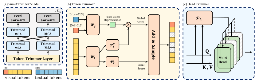
Figure 1: Overview of SmartTrim, best viewed in color. (a) SmartTrim collaborates with the VLM backbone to perform pruning by incorporating (b) token trimmer and (c) head trimmer.

1 Introduction

Transformer-based (Vaswani et al., 2017) pretrained vision-language models (VLMs) have shown great success in achieving superior performance on various vision-language (VL) tasks with their delicate model structures (Radford et al., 2021; Wang et al., 2022d; Chen et al., 2022). However, these models are commonly found to have long input sequences and vast amounts of parameters. Reducing such costs and improving model efficiency poses a crucial issue when landing them in real-world scenarios. The complexity of VL tasks varies significantly among different input instances. Input instances that involve complex cross-modal interaction naturally require a larger computational budget, while those with simpler cross-modal interaction typically demand a smaller budget. This contrast leads to the intuition that the computational overhead required for each instance is positively correlated with the complexity of its cross-modal interaction. However, previous work on VLMs (Fang et al., 2021; Wang et al., 2022c; Gan et al., 2022; Jiang et al., 2022; Shi et al., 2023) has focused mainly on static acceleration approaches, including pruning and distillation. We argue that these methods are sub-optimal since they fix the architecture during inference and treat all instances equally. In this work, we propose SmartTrim, an adaptive method that adjusts the computational overhead of the inference based on the complexity of inputs. Concretely, we introduce lightweight trimming modules, referred to as trimmers, into the backbone to perform pruning on tokens and attention heads, as shown in Figure 1. To maintain the ability of cross-modal interactions in the original model, the trimmers are cross-modal aware. They effectively identify tokens and parameters that are more relevant to cross-modal interaction by using global information from another modality in conjunction with their own information. We adopt the reparameterization method (Jang et al., 2017) to allow trimmers to be optimized jointly with the backbone network on downstream tasks without additional pre-training. To further alleviate the instability problem caused by adaptive pruning in the training phase, we propose curriculum training strategies, including stable initialization and the curriculum learning scheduler. In order to achieve a promising performance even at high speed-up ratios (more than $2\times$), we introduced a self-distillation objective during the task-specific fine-tuning process of SmartTrim. Unlike traditional knowledge distillation methods that require a large-scale fine-tuned teacher model, our approach averts this limitation by encouraging the trimmed model (with trimming masks) to align with the ability of the full model (without trimming masks).

We chose two representative pre-trained VLMs for experiments to demonstrate the generality of our approach: METER (Dou et al., 2022), which is an encoder-based architecture, and BLIP (Li et al., 2022), which is an encoder-decoder-based architecture. Experimental results on various vision-language tasks reveal that SmartTrim preserves the performance of $96\%$ to $99\%$ of the original VLMs while reducing computational overhead by more than $2\times$. Compared to other acceleration VLM methods, SmartTrim achieves better results and efficiency-performance trade-offs. Further analysis indicates that the cross-modal interaction information is crucial for adaptive pruning in VLMs. In addition, SmartTrim effectively learns to adaptively allocate more computational resources to complex instances while allocating fewer resources to simple instances.

2 Related Work

2.1 Vision-Language Pre-training

Pretrained vision-language models (VLM) have advanced the state of the art on various vision-language tasks. Previous VLMs (Li et al., 2019; Tan and Bansal, 2019; Lu et al., 2019; Chen et al., 2020b; Li et al., 2020; Cho et al., 2021; Zhang et al., 2021; Li et al., 2021b) rely on pretrained object detectors (Ren et al., 2015) to extract visual-region features, resulting in heavy computational overhead. Consequently, most of the recent work on VLM focuses on exploring fully Transformer-based architectures (Radford et al., 2021; Kim et al., 2021; Li et al., 2021a; Wang et al., 2021b, 2022b; Yu et al., 2022; Zeng et al., 2022; Xu et al., 2022a; Diao et al., 2022; Li et al., 2023). They directly employ vision Transformers (Dosovitskiy et al., 2021) to extract visual features and fuse them with textual features using a Transformer-based cross-modal encoder. Although large-scale Transformer-based VLMs achieve satisfactory performance, the extensive amount of parameters in both uni-modal and cross-modal encoders inflict an extravagant computational burden, impeding their scalability and application in the production environment.

2.2 Transformer Acceleration

Due to the high computational cost, extensive work has been proposed to accelerate Transformer for deployment on resource-limited devices (Xu et al., 2021). The existing work falls into lines: Static and Adaptive acceleration (Zhou et al., 2020).

Static Acceleration

The lightweight models obtained from static methods remain fixed for all instances during inference. Knowledge distillation (Hinton et al., 2015; Sanh et al., 2019; Sun et al., 2019; Jiao et al., 2020; Wang et al., 2020b; Zhou et al., 2022; Touvron et al., 2021; Fang et al., 2021; Wang et al., 2021c, 2022c), quantization (Shen et al., 2020) and module replacement (Xu et al., 2020) can be effectively accelerated Transformers. Pruning (LeCun et al., 1989) is also widely used for Transformer acceleration. Unstructured pruning (Han et al., 2015; Gordon et al., 2020) removes individual redundant neurons from the original model. These methods achieve high sparsity with competitive performance (Chen et al., 2020a; Prasanna et al., 2020; Gan et al., 2022), but with a negligible improvement in speed on general hardware (Ganesh et al., 2021). For better hardware efficiency, structured pruning focuses on removing structures (Hou et al., 2020; Lagunas et al., 2021; Xia et al., 2022), such as attention heads (Michel et al., 2019), feed-forward network (McCarley et al., 2019; Wang et al., 2020c) and entire layer Fan et al. (2020). Shi et al. (2023) propose to iterative progressive prune and retrain to find subnetworks on VL tasks.

Orthogonal to parameter compression, token pruning eliminates input tokens hierarchically to accelerate Transformer inference (Dai et al., 2020; Goyal et al., 2020; Chen et al., 2021; Rao et al., 2021; Ryoo et al., 2021; Tang et al., 2022b; Liang et al., 2022; Xu et al., 2022b). To the best of our knowledge, TRIPS (Jiang et al., 2022) is the only previous static token pruning work for VLM, using textual information to eliminate visual tokens during image encoding. However, TRIPS needs to pretrain from scratch, resulting in an expensive training overhead. Moreover, it fixes the retained token ratio of layers for all instances and use costly operation like top-k for selection (Wang et al., 2021a).

Static acceleration methods fix the architecture at inference, regardless of large variations in complexity across different instances, limiting their capacity and flexibility.

Adaptive Acceleration

allows the model to dynamically adjust the required computation per instance at inference (Graves, 2016). Dynamic token pruning leverages a learned module to remove redundant tokens to achieve an adaptive pruning rate, unlike static methods. However, directly applying previous work on uni-modal Transformers (Ye et al., 2021; Kim et al., 2022; Guan et al., 2022; Pan et al., 2021; Yin et al., 2022; Meng et al., 2022; Kong et al., 2022) to more complex VLMs is suboptimal, as they do not consider any cross-modal information when pruning tokens. Early exiting (Teerapittayanon et al., 2016; Zhou et al., 2020) proposes a halting mechanism to perform input-adaptive inference. Recently, Tang et al. (2022a) has explored applying this strategy to a VLM based on the encoder-decoder architecture. However, early exit can be viewed as a coarse-grained token pruning method with the constraint of pruning all tokens at the same layer, resulting in poorer performance compared to other adaptive methods (Guan et al., 2022). In this work, we explore to accelerate VLMs by adaptive pruning more fine-grained units: input tokens and parameter structures like attention heads.

3 Preliminary

The fully Transformer-based VLM has emerged as a dominant architecture for various vision-language tasks. In this section, we present an overview of this architecture, followed by an empirical analysis of its input and parameter redundancy.

3.1 Transformer-based VLM

Recent VLMs typically employ uni-modal encoders to extract visual and textual features, subsequently fusing them via a cross-modal encoder.

Uni-Modal Encoders

The visual encoder slices the input image into a flattened patch sequence and prepends a [I_CLS] token to the sequence. Then we sum the image patch embeddings and position embeddings to obtain the visual input embeddings ${\bm{I}}_{0}=\{{\bm{i}}_{0}\}_{i=1}^{N}$, where $N$ is the length of the visual sequence. The $L_{v}$-layer Transformer encodes ${\bm{I}}_{0}$ as: ${\bm{I}}_{l}=\mathrm{Enc}_{l}^{v}({\bm{I}}_{l-1}),l\in[1,L_{v}]$. Each layer consists of a multi-head self-attention (MSA) module and a feed-forward network (FFN) module. In particular, the MSA with $N_{h}$ heads computes the visual-modality attention among ${\bm{I}}_{l-1}$ as:

$$\mathrm{MSA}({\bm{I}}_{l-1})=[{\bm{A}}_{1}^{v}{\bm{V}}_{1}^{v},\dots,{\bm{A}}_{N_{h}}^{v}{\bm{V}}_{N_{h}}^{v}]{\bm{W}}_{l}^{O}$$ (1)

$${\bm{A}}_{i}^{v}=\mathrm{softmax}(\frac{{\bm{Q}}_{i}^{v}{\bm{K}}_{i}^{v\intercal}}{\sqrt{d_{h}}})$$ (2)

where $d_{h}$ is a scaling factor, ${\bm{Q}}_{i}^{v},{\bm{K}}_{i}^{v},{\bm{V}}_{i}^{v}$ are obtained by projecting ${\bm{I}}_{l-1}$ using parameters ${\bm{W}}_{l}^{Q},{\bm{W}}_{l}^{K},{\bm{W}}_{l}^{V}$, respectively. The textual encoder prepends a [T_CLS] to the input text and subsequently tokenizes it into a sequence of $M$ tokens. Similarly, the textual representations ${\bm{T}}_{l}$ are calculated as: ${\bm{T}}_{l}=\mathrm{Enc}_{l}^{t}({\bm{T}}_{l-1}),l\in[1,L_{t}]$.

Cross-Modal Encoder

first transforms the final representations of uni-modal encoders ${\bm{I}}_{L_{v}}$ and ${\bm{T}}_{L_{t}}$ into ${\bm{Z}}_{0}^{v}$ and ${\bm{Z}}_{0}^{t}$, respectively. Following previous work (Dou et al., 2022; Li et al., 2022), we adopt the co-attention mechanism to capture cross-modal interactions. Formally, the $l$-th layer of the encoder is denoted as $\mathrm{Enc}^{c}_{l}$, including separate parameters for visual and textual modalities. In addition to the MSA and FFN, each part has a multi-head cross-attention (MCA) module to interact with the other modality representations. Specifically, in the MCA module, the ${\bm{Q}}$ is from one modality (e.g., visual), while the ${\bm{K}},{\bm{V}}$ are from the other modality(e.g,, textual).

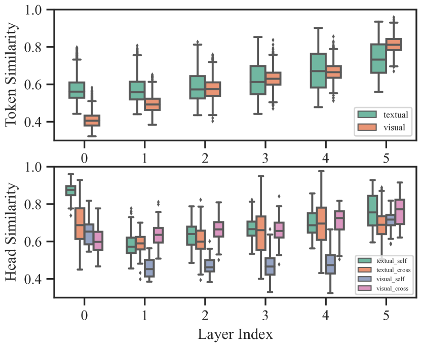
Figure 2: The token similarity (top) and head similarity (bottom) of the cross-modal encoder in METER fine-tuned on VQA dataset.

3.2 Empirical Analysis of Token and Parameter Redundancy in VLM

VLMs have long input sequences leading to substantial computational overheads, since the complexity of attention modules (MSAs or MCAs) scales quadratically to the sequence length. Large VLMs typically consist of hundreds of millions of parameters, burdening the situation even further. Previous findings (Goyal et al., 2020; Wang et al., 2022a) reveal that redundancy is present in the inputs and parameters (like attention heads) of BERT or ViT. To investigate whether redundancy also exists in VLMs, we fine-tune a typical model METER (Dou et al., 2022) on VQA, and measure cosine similarities between different tokens and different heads on each layer. Figure 2 shows results of the cross-modal encoder. We obtain the empirical findings as follows: (1) Similarities between tokens and heads are consistently high at all layers. (2) Token similarity increases progressively with the layer index, which indicates a growing redundancy in deeper layers. (3) Token similarity and head similarity vary exceptionally across instances, which motivates us to explore input-dependent adaptive pruning methods for VLMs.

4 Method

In this section, we propose SmartTrim, an adaptive acceleration framework for efficient VLMs by reducing redundant input tokens and attention heads. Figure 1 gives an overview of SmartTrim. We first present our adaptive trimmers for tokens and heads in SmartTrim. Then, we present our end-to-end training recipe for jointly optimizing the trimmers with the backbone.

4.1 Adaptive Trimmers

Cross-modal-aware Token Trimmer

As described in Section 3.2, redundancy exists in both visual and textual tokens and increases as the layer gets deeper. Therefore, we propose to progressively eliminate redundant tokens to save computational overhead. We achieve this by incorporating a lightweight token trimmer into each layer of the VLM backbone. The input features ${\bm{H}}\in\mathbb{R}^{N\times D}$ of $N$ tokens for each layer are first fed into the token trimmer, and the informative scores $\pi_{t}\in\mathbb{R}^{N}$ are calculated in a multi-grained manner. ${\bm{H}}$ are first projected by a linear layer to obtained ${\bm{H}}^{\prime}\in\mathbb{R}^{N\times D^{\prime}}$. The local informative scores $\pi^{l}_{t}$ are then obtained through the local policy network:

$$\pi_{t}^{l}=\mathcal{P}_{t}^{l}({\bm{H}}^{\prime})=\mathrm{MLP}({\bm{H}}^{\prime})$$ (3)

The local informative score $\pi_{t}^{l}$ only uses inner representation of each token to determine whether it is informative or not. However, local information is insufficient and may make sub-optimal decisions for the token trimming. We further propose to utilize the global information from self-modality and cross-modality. In particular, we use an MLP network to project visual and textual [CLS] tokens to acquire the fused global representation ${\bm{g}}$, which contains global information about both modalities:

$${\bm{g}}=\mathrm{MLP}([{\bm{c}}_{s},{\bm{c}}_{c}])$$ (4)

We then compute the bilinear similarity between ${\bm{g}}$ and ${\bm{H}}^{\prime}$ as the global informative score $\pi_{t}^{g}$:

$$\pi_{t}^{g}=\mathcal{P}_{t}^{g}({\bm{g}},{\bm{H}}^{\prime})={\bm{g}}{\bm{W}}_{k}{\bm{H}}^{\prime\intercal}$$ (5)

The final token informative score $\pi_{t}$ considers both the local score $\pi_{t}^{l}$ and the cross-modal-aware global score $\pi_{t}^{g}$: $\pi_{t}=\pi_{t}^{l}+\pi_{t}^{g}$. The token trimmer produce the trimming mask by the sigmoid activation:

$${\bm{M}}_{t}=\sigma(\pi_{t})$$ (6)

where the ${\bm{M}}_{t}$ is binary, and $0$ represents to discard the token and $1$ represents to keep.

Global Head Trimmer

In addition to the input tokens, we also observe a large redundancy between heads in different attention modules. Similar to token trimming, we propose global head trimmers to select more important heads by the global information of representations. Specifically, the trimmer takes [CLS] tokens in both modality to generate head trimming policy $\pi_{h}\in\mathbb{R}^{N_{h}}$ for each module:

$$\pi_{h}=\left\{\begin{aligned} &\mathcal{P}^{s}_{h}({\bm{c}}_{s})&(\text{MSA})\\ &\mathcal{P}^{c}_{h}([{\bm{c}}_{s},{\bm{c}}_{c}])&(\text{MCA})\end{aligned}\right.$$ (7)

Finally, the head trimmer use a sigmoid activation to generate binary masks.

4.2 Training Recipe

End-to-End Optimization

SmartTrim directly removes tokens and heads based on the masks ${\bm{M}}_{\textit{T}}$ and ${\bm{M}}_{\textit{H}}$ during inference. However, the binary masks are non-differentiable, bring challenges to end-to-end optimization in the training procedure. To address this problem, we adopt the reparameterization technique (Jang et al., 2017) to sample discrete masks ${\bm{M}}$ from the distributions $\bm{\pi}$:

$$\begin{split}{\bm{M}}&=\sigma((\bm{\pi}+{\bm{G}}^{\prime}-{\bm{G}}^{\prime\prime})/\tau)\\ &=\frac{\exp((\bm{\pi}+{\bm{G}}^{\prime})/\tau)}{\exp((\bm{\pi}+{\bm{G}}^{\prime})/\tau)+\exp({\bm{G}}^{\prime\prime}/\tau)}\\ \end{split}$$ (8)

where ${\bm{G}}^{\prime}$ and ${\bm{G}}^{\prime\prime}$ are two independent Gumbel noises, and $\tau$ is a a temperature factor.

To achieve a better efficiency-performance trade-off, we introduce a cost loss term $\mathcal{L}_{cost}$ as follows:

$$\mathcal{L}_{cost}=\frac{1}{|P|}\sum_{p\in P}(\beta_{p}-\gamma_{p})^{2}$$ (9)

where $\gamma_{p}$ is desired sparsity of module $p$, and the actual sparsity $\beta_{p}$ is defined as follows:

$$\beta_{p}=\left\{\begin{aligned} &\frac{1}{|p|}\sum_{t\in p}\frac{M_{t}}{N^{p}_{token}}&(\text{if}~{}p~{}\text{is}~{}token)\\ &\frac{1}{|p|}\sum_{h\in p}\frac{M_{h}}{N^{p}_{head}}&(\text{if}~{}p~{}\text{is}~{}head)\\ \end{aligned}\right.$$ (10)

Curriculum Training

Random initialization of adaptive pruning can corrupt the pretrained backbone, leading to the collapse of training. We propose the curriculum training strategies to improve the stability of model training, including: Stable Initialization to make sure that all tokens/heads are kept and avoid random selection at the beginning of training. Linear Curriculum Scheduler progressively decrease the $\gamma_{p}$ from $1.0$ to the target ratio after a predefined percentage of training.

Self-Distillation

As the sparsity increases, the inconsistency between the trimmed model and the full model grows. To overcome this issue, we introduce a self-distillation mechanism to transfer knowledge from the full capacity model to the pruned model by aligning their outputs. Given a trimmed network $f(x,P)$ where $x$ is input and $P$ is the set of activated trimmers. We encourage the $f(x,P)$ to make consistent prediction as the full capacity network $f(x,\varnothing)$. To this end, we minimize the KL-diversity between the prediction of $f(x,P)$ and $f(x,\varnothing)$:

$$\mathcal{L}_{SD} =\mathcal{L}_{task}(f(x,\varnothing),y)$$ (11)

$$+D_{KL}(f(x,P)||f(x,\varnothing))$$

The overall training objective is a combination of the above objectives:

$$\mathcal{L} =\mathcal{L}_{task}+\lambda_{SD}\mathcal{L}_{SD}+\lambda_{cost}\mathcal{L}_{cost}$$ (12)

5 Experiments

5.1 Setup

Tasks and Datasets

We conduct experiments on a wide range of visual-language downstream tasks: vision-language understanding on NLVR2 (Suhr et al., 2019), VQA (Goyal et al., 2017) and SNLI-VE (Xie et al., 2019), image-text retrieval on Flickr30K (Plummer et al., 2015), image captioning on COCO (Lin et al., 2014) and NoCaps (Agrawal et al., 2019). More details are presented in the Appendix B.

Baselines

We select two typical VLMs: METER (Dou et al., 2022), an encoder-based architecture, and BLIP (Li et al., 2022), an encoder-decoder-based architecture, as our backbones for adaptive pruning. In addition to the backbone models, we mainly compare our approach with baselines that require only task-specific fine-tuning. We implement a fine-tuning knowledge distillation baseline (FTKD): selecting layers from a pretrained backbone to initialize a smaller model and fine-tuning it with the same distillation objectives as (Jiao et al., 2020). We also employ the TRIPS (Jiang et al., 2022) framework on the METER backbone but only performing task-specific fine-tuning without pre-training.

For reference, we also provide results of several pretrained accelerated models including MiniVLM (Wang et al., 2020a), DistillVLM (Fang et al., 2021), $\text{X-VLM}_{\text{small}}$, EfficientVLM (Wang et al., 2022c) and TRIPS (Jiang et al., 2022).

Implementation Details

The resolution of the image for fine-tuning is $288^{2}$, unless otherwise stated. For other hyperparameters of METER and BLIP fine-tuning, we mainly follow their original settings. Following (Wang et al., 2022c), we set different target ratios for different modalities. We set the cost loss weight $\lambda_{cost}$ as $20.0$ and the self-distillation weight $\lambda_{SD}$ as $1.0$ for all experiments.

For efficiency measurement, we employ the widely used metric FLOPs, which is hardware independent. To prevent pseudo-improvement caused by pruning padding tokens, we evaluate models with the input without padding (single instance usage), similarly to previous work (Ye et al., 2021; Modarressi et al., 2022).

Methods	NLVR2		VQA	SNLI-VE		ITR		FLOPs(G)
	dev	test-P	test-dev	val	test	IR	TR
METER (backbone)	82.05	82.32	76.78	80.87	80.83	92.1	97.7	48.3
(a) Acceleration Methods Need Pre-training
MiniVLM	73.71	73.93	69.10	-	-	-	-	-
DistillVLM	-	-	69.80	-	-	-	-	-
$\text{X-VLM}_{\text{small}}$	79.34	79.26	73.70	-	-	-	-	-
EfficientVLM	81.83	81.72	76.20	-	-	-	-	-
TRIPS	82.35	83.34	76.23	-	-	94.3	98.7	-
(b) Acceleration Methods Only Need Task-specific Fine-tuning
$\text{TRIPS}_{1.5\times}^{{\dagger}}$	81.34	82.01	76.30	80.55	80.87	91.6	97.4	32.1
$\textsc{SmartTrim}_{1.5\times}$	81.89	82.72	76.56	80.79	80.60	91.6	97.8	31.1
$\text{FTKD}_{2.0\times}$	76.89	77.49	67.82	76.89	77.14	-	-	26.0
$\text{TRIPS}_{2.0\times}^{{\dagger}}$	80.42	81.35	75.33	80.28	80.39	90.0	96.5	25.7
$\textsc{SmartTrim}_{2.0\times}$	82.02	81.97	76.44	80.58	80.63	90.5	97.5	26.2
$\text{FTKD}_{3.0\times}$	65.86	67.10	58.74	72.97	73.19	-	-	17.7
$\text{TRIPS}_{2.5\times}^{{\dagger}}$	77.90	78.91	71.88	79.44	79.52	86.5	94.1	17.9
$\textsc{SmartTrim}_{2.5\times}$	81.18	81.55	75.50	80.20	80.24	89.0	96.4	18.6

Table 1: Evaluation results on various vision-language tasks. We report the mean recall metrics for image retrieval (IR) and text retrieval (TR). The results are averaged over 3 runs. The METER backbone is fine-tuned on image with $288^{2}$ resolution. FTKD, TRIPS^† and SmartTrim are our implementation based on METER and fine-tuned on $288^{2}$-resolution images with the same hyper-parameters. The results in Group (a) are not directly comparable due to different backbones, resolutions, and the need for large-scale pre-training in their approaches.

Methods	NLVR2			VQA
	dev	test-P	FLOPs(G)	test-dev	FLOPs(G)
BLIP	81.64	81.98	71.2	75.72	38.6
$\textsc{SmartTrim}{}_{1.3\times}$	82.15	81.68	58.7	75.67	31.1
$\textsc{SmartTrim}{}_{1.5\times}$	82.01	81.90	48.2	75.34	24.4
$\textsc{SmartTrim}{}_{2.0\times}$	81.48	80.86	34.9	74.36	19.2

Table 2: Results of BLIP-based methods on NLVR2 and VQA. The models are fine-tuned on $288^{2}$-resolution images. We do not use additional VG datasets for VQA fine-tuning.

Methods	COCO FT		NoCaps ZS		FLOPs(G)
	B@4	C	C	S
BLIP	39.3	131.3	107.9	14.5	246.3
$\textsc{SmartTrim}{}_{1.3\times}$	39.6	132.3	107.8	14.5	206.6
$\textsc{SmartTrim}{}_{1.5\times}$	39.3	129.1	107.6	14.4	173.5
$\textsc{SmartTrim}{}_{2.0\times}$	38.1	125.4	105.6	14.3	121.1

Table 3: Image captioning results based on BLIP model. The models are fine-tuned on $288^{2}$-resolution images. All methods optimize the cross-entropy loss during fine-tuning. B@4: BLEU@4, C: CIDEr, S: SPICE.

5.2 Experimental Results

Main Results

Table 1 presents the performance of METER-based methods on various vision-language tasks. We observe that SmartTrim achieves competitive performance compared to the backbone METER (retaining $98\%$-$99\%$ performance) while reducing the computational overhead more than $2\times$. SmartTrim outperforms static baselines FTKD and TRIPS, and the advantage is more significant at high speed-up ratios, reflecting the effectiveness of our adaptive pruning. Our method also achieves performance comparable to some pretrained accelerated VLMs, which may indicate that our method is more economical.

We further perform SmartTrim on BLIP, another encoder-decoder-based VLM, and present the results in Tables 2 and 3. Interestingly, we observe that $\textsc{SmartTrim}_{1.3\times}$ performs better than the original BLIP, while reducing the computational cost by $16\%$~$20\%$. Notably, even by reducing the computational cost $50\%$, SmartTrim only has a slight degradation of $0.2\%$~$1.8\%$ in vision-language understanding and $1.4\%$~$4.5\%$ in image captioning, demonstrating the generality of our approach with consistent performance across architectures.

Figure 3: Pareto front of the efficiency-performance trade-off on NLVR2. The image resolution is $288^{2}$ by default unless specified in the subscript. SmartTrim achieve a better trade-off compared to other methods.

Models	VQA test-dev	FLOPs(G)	Latency
METER	76.78	48.30	343ms
$\text{FTKD}_{2.0\times}$	67.82	26.0	192ms
$\textsc{SmartTrim}{}_{2.0\times}$	76.44	26.2	214ms
$\text{FTKD}_{3.0\times}$	58.74	17.7	129ms
$\textsc{SmartTrim}{}_{3.0\times}$	75.18	17.3	178ms

Table 4: Averaged latency on VQA for models based on METER. We also report the VQA score and FLOPs of models for comparison.

Efficiency-Performance Trade-off

We further present a Pareto front of the efficiency-performance trade-off on the NLVR2 task in Figure 3. We find that between $1.2\times$ to $1.5\times$, our method gains more accuracy than the backbone while enjoying a "free lunch" in speedup. Furthermore, SmartTrim achieves a better efficiency-performance trade-off, maintaining competitive results at higher acceleration ratios, such as $3.0\times$. SmartTrim is also orthogonal to other acceleration methods, such as knowledge distillation. A potential direction for future work is to combine our adaptive pruning approach with other methods to further accelerate VLMs.

We evaluate the latency of SmartTrim and two baselines: the original model and FTKD. Similar to the FLOPs measurement, the evaluations are conducted under the setting of single-instance inference. The averaged latency is calculated using the VQA validation set on an Intel Xeon E5-2640 v4 CPU and reported in Table 4, including VQA performance and FLOPs for a better comparison. We find that both SmartTrim and FTKD significantly reduce inference latency compared to the original METER. With similar FLOPs, SmartTrim exhibits slightly higher latency than FTKD, mainly because FTKD directly reduces the depth of model. However, we observe that under a more aggressive acceleration setting (the bottom part of Table 4), FTKD suffers severe performance degradation since it restricts the backbone capacity. On the contrary, our method adaptively adjusts the capacity depending on the complexity of input samples and yields promising results. This phenomenon demonstrates the versatility of SmartTrim under different constraints, suggesting a strong potential for widespread applications.

Models	Image	VQA	FLOPs(G)
	Resolution	test-dev
METER	$288^{2}$	76.78	48.3
METER	$384^{2}$	77.37	88.5
$\textsc{SmartTrim}{}_{1.5\times}$	$384^{2}$	77.25	61.5
$\textsc{SmartTrim}{}_{2.0\times}$	$384^{2}$	77.10	46.0

Table 5: Results of models fine-tuned on VQA with different image resolution. SmartTrim models are based on METER.

Fine-tuning with higher resolution

Fine-tuning VLMs at higher resolution tends to improve performance (Dou et al., 2022). We fine-tune SmartTrim and the baseline METER with different resolutions on VQA and the results are presented in Table 5. We observe that increasing the image resolution from $288^{2}$ to $384^{2}$ improves the performance of baseline METER but sacrifices efficiency (doubling of FLOPs), which poses a challenge in the utilization of longer inputs. However, with a similar computational cost, SmartTrim fine-tuned on $384^{2}$ resolution achieves better performance than baselines. The observation indicates that through adaptive pruning redundant tokens and heads, SmartTrim is capable of encoding much longer sequences to gain better performance with less computation.

6 Analysis

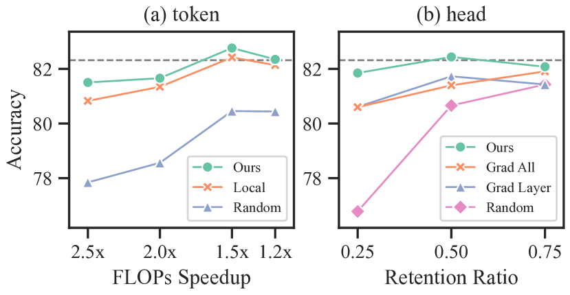
Figure 4: Comparison between different token (left) and head (right) pruning approaches on NLVR2. The dashed line denotes the performance of original METER.

6.1 Ablation Study

Effectiveness of Adaptive Trimmers

We first investigate the effectiveness of our proposed adaptive trimmers for tokens and heads in SmartTrim, respectively. For token pruning, we compare our method with other token pruning approaches: the Local baseline that prunes tokens solely based on their representations without incorporating cross-modal global representations, and the Random baseline that randomly samples a number of tokens to prune. For a fair comparison, the models are targeted at the same inference cost and fine-tuned with the same hyper-parameters on NLVR2. As shown in Figure 4(a), our method consistently outperforms other methods at different computational overheads.

For head pruning, we compare our method with two other head pruning approaches: the random baseline and the gradient-based baseline (Michel et al., 2019). For a given retention ratio $p\%$ of the entire model, the random baseline randomly retains $p\%$ of heads in each attention module. For the gradient-based baseline, we introduce two variants: (1) Grad Layer, which retains the top-$p\%$ heads in each attention module by importance score, (2) Grad All, which maintains the top-$p\%$ heads of the entire model. We apply these methods on the METER cross-modal encoder and fine-tune them on NLVR2. For more clarity, the models are trained without self-distillation. Figure 4(b) shows the evaluation results with different retention ratios. We observe that our adaptive head trimmer achieves the best accuracy at different ratios, which shows the effectiveness of our method. Furthermore, the gap between our method and the baseline gradually increases as the retention rate decreases, indicating the strong robustness of our method.

Models	NLVR2		VQA
	dev	test-P	test-dev
$\textsc{SmartTrim}{}_{1.5\times}$	81.89	82.72	76.56
- Stable Initialization	50.85	51.07	74.72
- Curriculum Scheduler	81.70	82.52	76.20
- Self-Distillation	81.25	82.15	76.36
$\textsc{SmartTrim}{}_{2.0\times}$	82.02	81.97	76.44
- Stable Initialization	50.85	51.07	74.34
- Curriculum Scheduler	81.58	82.01	75.59
- Self-Distillation	81.35	81.54	76.08
$\textsc{SmartTrim}{}_{2.5\times}$	81.18	81.55	75.50
- Stable Initialization	50.85	51.07	73.43
- Curriculum Scheduler	50.85	51.07	74.25
- Self-Distillation	80.51	81.30	74.70

Table 6: Ablation studies of SmartTrim training strategies. Average fine-tuning results of three random seeds are reported.

Effects of Training Strategies

We further perform ablation studies to analyze the contribution of our proposed training strategies. Table 6 shows that all of our strategies are beneficial for SmartTrim training. Specifically, the proposed curriculum training, including stable initialization and linear curriculum scheduler, effectively mitigates the instability in model training, without performance degradation even at high speedup ratio (e.g., $2.5\times$). Furthermore, the objective of self-distillation is crucial to maintain performance in various speed-up ratios, allowing SmartTrim to achieve a better trade-off between efficiency and performance.

6.2 Qualitative Analysis

Visualization of Token Trimming

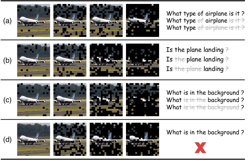
Figure 5: The visualization examples of token trimming process on VQA. From left to right, we show the visual and textual input tokens are progressively trimmed. (a)-(c) are obtained by the model incorporating the cross-modal-aware token trimmer. (d) is obtained by the local baseline that trims tokens without cross-modal information.

We first visualize the trimming masks generated by our proposed cross-modal-aware token trimmer in Figure 5. It can be observed that as the depth increases (from left to right), redundant visual and textual tokens are progressively trimmed. Notably, from figures 5(a)-(c), we discover that when provided with different textual inputs, our method utilize cross-modal interaction information to efficiently identify relevant patches. For comparison, we provide results of the local-only baseline in Figure 5 (d), which has the same input as (c). It may be observed that unlike SmartTrim which is guided by cross-modal information, the local trimmer is only capable of retaining the primary subject of the image, however irrelevant to the question. Additional visualization results can be found in the Appendix D.

Distribution of Trimmed Heads

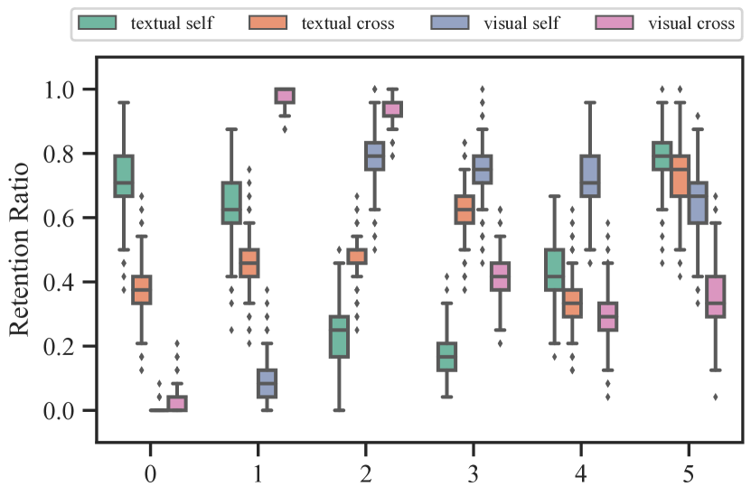
Figure 6: The layer-wise head retention ratio distribution of each attention module across the METER cross-modal encoder with target retention ratio $0.5$ on NLVR2.

We plot the layer-wise distribution of head masks in each attention module in Figure 6, with a target retention ratio of $0.5$. The actual retention ratio of head masks for the same layer varies greatly between instances. For different attention modules, significant variation can be perceived similarly in the layer-wise distribution.

Distribution of Computational Overhead

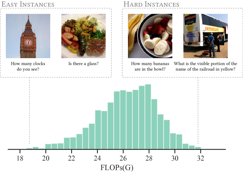
Figure 7: The distribution of computational overhead for instances in VQA validation dataset. We sample some instances allocated with least or most computations.

The previous analysis has shown that SmartTrim can leverage cross-modal information to adaptively derive trimming decisions on tokens or heads in the VLM. We further analyze the distribution of computations allocated by $\textsc{SmartTrim}{}_{2.0\times}$ in Figure 7, in which a large disparity in computational overhead can be observed among instances. Note that input instances with simpler images and problems tend to impose less computational overhead, while more complex instances require complex cross-modal interactions and as a consequence, demand more computing resources. This phenomenon demonstrated in Figure 7 empirically validate our motivation of adaptively adjusting computational budget based on the complexity of cross-modal interactions implied by input instances.

7 Conclusion

In this work, we propose SmartTrim, an adaptive pruning method for efficient VLMs that adjusts the inference overhead based on the complexity of instances. SmartTrim introduces lightweight trimming modules that leverage information from cross-modal interaction to prune redundant input tokens and parameters. Our method performs task-specific fine-tuning in conjunction with our proposed curriculum training and self-distillation strategies, without additional pre-training. Experimental results on various vision-language tasks show that SmartTrim achieves competitive performance with more than $2\times$ speed-up over backbone VLMs. When compared to previous acceleration approaches, SmartTrim achieves a better efficiency-performance trade-off. Further analysis illustrates that cross-modal information is critical in adaptive trimming for VLMs.

Appendix A Details of Similarity Calculation

Inspried by previous work (Goyal et al., 2020; Wang et al., 2022a), we calculate the average cosine similarity between token features and attention maps at each layer.

Token Similarity

Given the corresponding token features ${\bm{X}}\in\mathbb{R}^{N\times D}$, the averaged token similarity is computed by:

$${\bm{S}}_{\textit{T}}=\frac{2}{N(N-1)}\sum_{i=1}^{N}\sum_{j=i+1}^{N}\frac{{\bm{X}}_{i}\cdot{\bm{X}}_{j}}{\left\lVert{\bm{X}}_{i}\right\rVert_{2}\left\lVert{\bm{X}}_{j}\right\rVert_{2}}$$

Head Similarity

We use the similar metric to compute head similarity for attention maps. Given the attention map ${\bm{A}}\in\mathbb{R}^{H\times N\times N}$ with $H$ heads, the averaged cosine similarity between different heads is calculated as:

$${\bm{S}}_{\textit{A}}=\frac{2}{H(H-1)N}\sum_{i=1}^{H}\sum_{j=i+1}^{H}\sum_{k=1}^{N}\frac{{\bm{A}}_{i}^{k}\cdot{\bm{A}}_{j}^{k}}{\left\lVert{\bm{A}}_{i}^{k}\right\rVert_{2}\left\lVert{\bm{A}}_{j}^{k}\right\rVert_{2}}$$

where ${\bm{A}}_{i}^{k}$ denotes the $k$-th token’s attention distribution in the $i$-th head.

Appendix B Details of Downstream Tasks

Natural Language for Visual Reasoning

(NLVR2 Suhr et al. (2019)) is a visual reasoning task that aims to determine whether a textual statement describes a pair of images. For METER-based models, we construct two pairs of image-text, each consisting of the image and a textual statement. For models based on BLIP, we directly feed the two images and the text to the encoder.

Visual Question Answering

(VQA v2 (Goyal et al., 2017)) requires the model to answer questions based on the input image. For METER-based models, we formulate the problem as a classification task with 3,129 answer candidates. For BLIP-based models, we consider it as an answer generation task and use the decoder to rank the candidate answers during inference. Note that we did not use any additional training data from Visual Genome.

Visual Entailment

(SNLI-VE (Xie et al., 2019)) is a three-way classification dataset, aiming to predict the relationship between an image and a text hypothesis: entailment, natural, and contradiction.

Image-Text Retrieval

(ITR) We evaluate image-to-text retrieval (TR) and text-to-image retrieval (IR) on Flickr30K (Plummer et al., 2015) with the standard split (Karpathy and Fei-Fei, 2015).

Image Captioning

The image is given to the encoder and the decoder will generate the corresponding caption with a text prompt "a picture of" following Li et al. (2022). Our experiments are conducted on COCO (Lin et al., 2014), and the evaluation is performed on both the COCO test set and the NoCaps (Agrawal et al., 2019) validation set (zero-shot transfer).

Appendix C Details of Gradient-based Head Pruning

Gradient-based head pruning (Michel et al., 2019) first computes loss on pseudo-labels and then prunes attention heads with the importance score obtained by Taylor expansion. With given input $x$, importance score of head $h$ is defined as:

$${\bm{I}}_{\textit{h}}=E_{x}\left|A_{h}^{T}\frac{\partial\mathcal{L}(x)}{\partial A_{h}}\right|$$

Where $\mathcal{L}$ is the loss function, and $A_{h}$ is the context layer of head $h$.

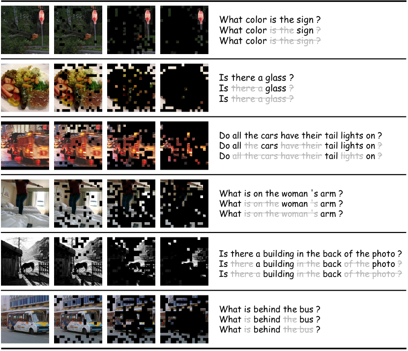
Figure 8: More visualization results by SmartTrim.

Appendix D More Visualization Examples

To demonstrate the ability to understand cross-modal interactions of our approach, we show additional visualization results of the token mask in Figure 8 using the same setting described in section 6.2.

References

- Agrawal et al. (2019) Harsh Agrawal, Peter Anderson, Karan Desai, Yufei Wang, Xinlei Chen, Rishabh Jain, Mark Johnson, Dhruv Batra, Devi Parikh, and Stefan Lee. 2019. nocaps: novel object captioning at scale. In 2019 IEEE/CVF International Conference on Computer Vision, ICCV 2019, Seoul, Korea (South), October 27 - November 2, 2019, pages 8947–8956. IEEE.
- Chen et al. (2021) Tianlong Chen, Yu Cheng, Zhe Gan, Lu Yuan, Lei Zhang, and Zhangyang Wang. 2021. Chasing sparsity in vision transformers: An end-to-end exploration. In Advances in Neural Information Processing Systems 34: Annual Conference on Neural Information Processing Systems 2021, NeurIPS 2021, December 6-14, 2021, virtual, pages 19974–19988.
- Chen et al. (2020a) Tianlong Chen, Jonathan Frankle, Shiyu Chang, Sijia Liu, Yang Zhang, Zhangyang Wang, and Michael Carbin. 2020a. The lottery ticket hypothesis for pre-trained BERT networks. In Advances in Neural Information Processing Systems 33: Annual Conference on Neural Information Processing Systems 2020, NeurIPS 2020, December 6-12, 2020, virtual.
- Chen et al. (2022) Xi Chen, Xiao Wang, Soravit Changpinyo, A. J. Piergiovanni, Piotr Padlewski, Daniel Salz, Sebastian Goodman, Adam Grycner, Basil Mustafa, Lucas Beyer, Alexander Kolesnikov, Joan Puigcerver, Nan Ding, Keran Rong, Hassan Akbari, Gaurav Mishra, Linting Xue, Ashish Thapliyal, James Bradbury, Weicheng Kuo, Mojtaba Seyedhosseini, Chao Jia, Burcu Karagol Ayan, Carlos Riquelme, Andreas Steiner, Anelia Angelova, Xiaohua Zhai, Neil Houlsby, and Radu Soricut. 2022. Pali: A jointly-scaled multilingual language-image model. CoRR, abs/2209.06794.
- Chen et al. (2020b) Yen-Chun Chen, Linjie Li, Licheng Yu, Ahmed El Kholy, Faisal Ahmed, Zhe Gan, Yu Cheng, and Jingjing Liu. 2020b. UNITER: universal image-text representation learning. In Computer Vision - ECCV 2020 - 16th European Conference, Glasgow, UK, August 23-28, 2020, Proceedings, Part XXX, volume 12375 of Lecture Notes in Computer Science, pages 104–120. Springer.
- Cho et al. (2021) Jaemin Cho, Jie Lei, Hao Tan, and Mohit Bansal. 2021. Unifying vision-and-language tasks via text generation. In Proceedings of the 38th International Conference on Machine Learning, ICML 2021, 18-24 July 2021, Virtual Event, volume 139 of Proceedings of Machine Learning Research, pages 1931–1942. PMLR.
- Dai et al. (2020) Zihang Dai, Guokun Lai, Yiming Yang, and Quoc Le. 2020. Funnel-transformer: Filtering out sequential redundancy for efficient language processing. In Advances in Neural Information Processing Systems 33: Annual Conference on Neural Information Processing Systems 2020, NeurIPS 2020, December 6-12, 2020, virtual.
- Diao et al. (2022) Shizhe Diao, Wangchunshu Zhou, Xinsong Zhang, and Jiawei Wang. 2022. Prefix language models are unified modal learners. CoRR, abs/2206.07699.
- Dosovitskiy et al. (2021) Alexey Dosovitskiy, Lucas Beyer, Alexander Kolesnikov, Dirk Weissenborn, Xiaohua Zhai, Thomas Unterthiner, Mostafa Dehghani, Matthias Minderer, Georg Heigold, Sylvain Gelly, Jakob Uszkoreit, and Neil Houlsby. 2021. An image is worth 16x16 words: Transformers for image recognition at scale. In 9th International Conference on Learning Representations, ICLR 2021, Virtual Event, Austria, May 3-7, 2021. OpenReview.net.
- Dou et al. (2022) Zi-Yi Dou, Yichong Xu, Zhe Gan, Jianfeng Wang, Shuohang Wang, Lijuan Wang, Chenguang Zhu, Pengchuan Zhang, Lu Yuan, Nanyun Peng, Zicheng Liu, and Michael Zeng. 2022. An empirical study of training end-to-end vision-and-language transformers.
- Fan et al. (2020) Angela Fan, Edouard Grave, and Armand Joulin. 2020. Reducing transformer depth on demand with structured dropout. In 8th International Conference on Learning Representations, ICLR 2020, Addis Ababa, Ethiopia, April 26-30, 2020. OpenReview.net.
- Fang et al. (2021) Zhiyuan Fang, Jianfeng Wang, Xiaowei Hu, Lijuan Wang, Yezhou Yang, and Zicheng Liu. 2021. Compressing visual-linguistic model via knowledge distillation. In 2021 IEEE/CVF International Conference on Computer Vision, ICCV 2021, Montreal, QC, Canada, October 10-17, 2021, pages 1408–1418. IEEE.
- Gan et al. (2022) Zhe Gan, Yen-Chun Chen, Linjie Li, Tianlong Chen, Yu Cheng, Shuohang Wang, Jingjing Liu, Lijuan Wang, and Zicheng Liu. 2022. Playing lottery tickets with vision and language. In Thirty-Sixth AAAI Conference on Artificial Intelligence, AAAI 2022, Thirty-Fourth Conference on Innovative Applications of Artificial Intelligence, IAAI 2022, The Twelveth Symposium on Educational Advances in Artificial Intelligence, EAAI 2022 Virtual Event, February 22 - March 1, 2022, pages 652–660. AAAI Press.
- Ganesh et al. (2021) Prakhar Ganesh, Yao Chen, Xin Lou, Mohammad Ali Khan, Yin Yang, Hassan Sajjad, Preslav Nakov, Deming Chen, and Marianne Winslett. 2021. Compressing large-scale transformer-based models: A case study on BERT. Trans. Assoc. Comput. Linguistics, 9:1061–1080.
- Gordon et al. (2020) Mitchell A. Gordon, Kevin Duh, and Nicholas Andrews. 2020. Compressing BERT: studying the effects of weight pruning on transfer learning. In Proceedings of the 5th Workshop on Representation Learning for NLP, RepL4NLP@ACL 2020, Online, July 9, 2020, pages 143–155. Association for Computational Linguistics.
- Goyal et al. (2020) Saurabh Goyal, Anamitra Roy Choudhury, Saurabh Raje, Venkatesan T. Chakaravarthy, Yogish Sabharwal, and Ashish Verma. 2020. Power-bert: Accelerating BERT inference via progressive word-vector elimination. In Proceedings of the 37th International Conference on Machine Learning, ICML 2020, 13-18 July 2020, Virtual Event, volume 119 of Proceedings of Machine Learning Research, pages 3690–3699. PMLR.
- Goyal et al. (2017) Yash Goyal, Tejas Khot, Douglas Summers-Stay, Dhruv Batra, and Devi Parikh. 2017. Making the V in VQA matter: Elevating the role of image understanding in visual question answering. In 2017 IEEE Conference on Computer Vision and Pattern Recognition, CVPR 2017, Honolulu, HI, USA, July 21-26, 2017, pages 6325–6334. IEEE Computer Society.
- Graves (2016) Alex Graves. 2016. Adaptive computation time for recurrent neural networks. CoRR, abs/1603.08983.
- Guan et al. (2022) Yue Guan, Zhengyi Li, Jingwen Leng, Zhouhan Lin, and Minyi Guo. 2022. Transkimmer: Transformer learns to layer-wise skim. In Proceedings of the 60th Annual Meeting of the Association for Computational Linguistics (Volume 1: Long Papers), ACL 2022, Dublin, Ireland, May 22-27, 2022, pages 7275–7286. Association for Computational Linguistics.
- Han et al. (2015) Song Han, Jeff Pool, John Tran, and William J. Dally. 2015. Learning both weights and connections for efficient neural network. In Advances in Neural Information Processing Systems 28: Annual Conference on Neural Information Processing Systems 2015, December 7-12, 2015, Montreal, Quebec, Canada, pages 1135–1143.
- Hinton et al. (2015) Geoffrey E. Hinton, Oriol Vinyals, and Jeffrey Dean. 2015. Distilling the knowledge in a neural network. CoRR, abs/1503.02531.
- Hou et al. (2020) Lu Hou, Zhiqi Huang, Lifeng Shang, Xin Jiang, Xiao Chen, and Qun Liu. 2020. Dynabert: Dynamic BERT with adaptive width and depth. In Advances in Neural Information Processing Systems 33: Annual Conference on Neural Information Processing Systems 2020, NeurIPS 2020, December 6-12, 2020, virtual.
- Jang et al. (2017) Eric Jang, Shixiang Gu, and Ben Poole. 2017. Categorical reparameterization with gumbel-softmax. In 5th International Conference on Learning Representations, ICLR 2017, Toulon, France, April 24-26, 2017, Conference Track Proceedings. OpenReview.net.
- Jiang et al. (2022) Chaoya Jiang, Haiyang Xu, Chenliang Li, Ming Yan, Wei Ye, Shikun Zhang, Bin Bi, and Songfang Huang. 2022. TRIPS: efficient vision-and-language pre-training with text-relevant image patch selection. In Proceedings of the 2022 Conference on Empirical Methods in Natural Language Processing, EMNLP 2022, Abu Dhabi, United Arab Emirates, December 7-11, 2022, pages 4084–4096. Association for Computational Linguistics.
- Jiao et al. (2020) Xiaoqi Jiao, Yichun Yin, Lifeng Shang, Xin Jiang, Xiao Chen, Linlin Li, Fang Wang, and Qun Liu. 2020. Tinybert: Distilling BERT for natural language understanding. In Findings of the Association for Computational Linguistics: EMNLP 2020, Online Event, 16-20 November 2020, volume EMNLP 2020 of Findings of ACL, pages 4163–4174. Association for Computational Linguistics.
- Karpathy and Fei-Fei (2015) Andrej Karpathy and Li Fei-Fei. 2015. Deep visual-semantic alignments for generating image descriptions. In IEEE Conference on Computer Vision and Pattern Recognition, CVPR 2015, Boston, MA, USA, June 7-12, 2015, pages 3128–3137. IEEE Computer Society.
- Kim et al. (2022) Sehoon Kim, Sheng Shen, David Thorsley, Amir Gholami, Woosuk Kwon, Joseph Hassoun, and Kurt Keutzer. 2022. Learned token pruning for transformers. In KDD ’22: The 28th ACM SIGKDD Conference on Knowledge Discovery and Data Mining, Washington, DC, USA, August 14 - 18, 2022, pages 784–794. ACM.
- Kim et al. (2021) Wonjae Kim, Bokyung Son, and Ildoo Kim. 2021. Vilt: Vision-and-language transformer without convolution or region supervision. In Proceedings of the 38th International Conference on Machine Learning, volume 139 of Proceedings of Machine Learning Research, pages 5583–5594. PMLR.
- Kong et al. (2022) Zhenglun Kong, Peiyan Dong, Xiaolong Ma, Xin Meng, Wei Niu, Mengshu Sun, Xuan Shen, Geng Yuan, Bin Ren, Hao Tang, Minghai Qin, and Yanzhi Wang. 2022. Spvit: Enabling faster vision transformers via latency-aware soft token pruning. In Computer Vision - ECCV 2022 - 17th European Conference, Tel Aviv, Israel, October 23-27, 2022, Proceedings, Part XI, volume 13671 of Lecture Notes in Computer Science, pages 620–640. Springer.
- Lagunas et al. (2021) François Lagunas, Ella Charlaix, Victor Sanh, and Alexander M. Rush. 2021. Block pruning for faster transformers. In Proceedings of the 2021 Conference on Empirical Methods in Natural Language Processing, EMNLP 2021, Virtual Event / Punta Cana, Dominican Republic, 7-11 November, 2021, pages 10619–10629. Association for Computational Linguistics.
- LeCun et al. (1989) Yann LeCun, John S. Denker, and Sara A. Solla. 1989. Optimal brain damage. In Advances in Neural Information Processing Systems 2, [NIPS Conference, Denver, Colorado, USA, November 27-30, 1989], pages 598–605. Morgan Kaufmann.
- Li et al. (2023) Junnan Li, Dongxu Li, Silvio Savarese, and Steven C. H. Hoi. 2023. BLIP-2: bootstrapping language-image pre-training with frozen image encoders and large language models. CoRR, abs/2301.12597.
- Li et al. (2022) Junnan Li, Dongxu Li, Caiming Xiong, and Steven C. H. Hoi. 2022. BLIP: bootstrapping language-image pre-training for unified vision-language understanding and generation. In International Conference on Machine Learning, ICML 2022, 17-23 July 2022, Baltimore, Maryland, USA, volume 162 of Proceedings of Machine Learning Research, pages 12888–12900. PMLR.
- Li et al. (2021a) Junnan Li, Ramprasaath R. Selvaraju, Akhilesh Deepak Gotmare, Shafiq R. Joty, Caiming Xiong, and Steven C. H. Hoi. 2021a. Align before fuse: Vision and language representation learning with momentum distillation. CoRR, abs/2107.07651.
- Li et al. (2019) Liunian Harold Li, Mark Yatskar, Da Yin, Cho-Jui Hsieh, and Kai-Wei Chang. 2019. Visualbert: A simple and performant baseline for vision and language. CoRR, abs/1908.03557.
- Li et al. (2021b) Wei Li, Can Gao, Guocheng Niu, Xinyan Xiao, Hao Liu, Jiachen Liu, Hua Wu, and Haifeng Wang. 2021b. UNIMO: towards unified-modal understanding and generation via cross-modal contrastive learning. In Proceedings of the 59th Annual Meeting of the Association for Computational Linguistics and the 11th International Joint Conference on Natural Language Processing, ACL/IJCNLP 2021, (Volume 1: Long Papers), Virtual Event, August 1-6, 2021, pages 2592–2607. Association for Computational Linguistics.
- Li et al. (2020) Xiujun Li, Xi Yin, Chunyuan Li, Pengchuan Zhang, Xiaowei Hu, Lei Zhang, Lijuan Wang, Houdong Hu, Li Dong, Furu Wei, Yejin Choi, and Jianfeng Gao. 2020. Oscar: Object-semantics aligned pre-training for vision-language tasks. In Computer Vision - ECCV 2020 - 16th European Conference, Glasgow, UK, August 23-28, 2020, Proceedings, Part XXX, volume 12375 of Lecture Notes in Computer Science, pages 121–137. Springer.
- Liang et al. (2022) Youwei Liang, Chongjian Ge, Zhan Tong, Yibing Song, Jue Wang, and Pengtao Xie. 2022. Evit: Expediting vision transformers via token reorganizations. In The Tenth International Conference on Learning Representations, ICLR 2022, Virtual Event, April 25-29, 2022. OpenReview.net.
- Lin et al. (2014) Tsung-Yi Lin, Michael Maire, Serge J. Belongie, James Hays, Pietro Perona, Deva Ramanan, Piotr Dollár, and C. Lawrence Zitnick. 2014. Microsoft COCO: common objects in context. In Computer Vision - ECCV 2014 - 13th European Conference, Zurich, Switzerland, September 6-12, 2014, Proceedings, Part V, volume 8693 of Lecture Notes in Computer Science, pages 740–755. Springer.
- Lu et al. (2019) Jiasen Lu, Dhruv Batra, Devi Parikh, and Stefan Lee. 2019. Vilbert: Pretraining task-agnostic visiolinguistic representations for vision-and-language tasks. In Advances in Neural Information Processing Systems 32: Annual Conference on Neural Information Processing Systems 2019, NeurIPS 2019, December 8-14, 2019, Vancouver, BC, Canada, pages 13–23.
- McCarley et al. (2019) JS McCarley, Rishav Chakravarti, and Avirup Sil. 2019. Structured pruning of a bert-based question answering model. arXiv preprint arXiv:1910.06360.
- Meng et al. (2022) Lingchen Meng, Hengduo Li, Bor-Chun Chen, Shiyi Lan, Zuxuan Wu, Yu-Gang Jiang, and Ser-Nam Lim. 2022. Adavit: Adaptive vision transformers for efficient image recognition. In IEEE/CVF Conference on Computer Vision and Pattern Recognition, CVPR 2022, New Orleans, LA, USA, June 18-24, 2022, pages 12299–12308. IEEE.
- Michel et al. (2019) Paul Michel, Omer Levy, and Graham Neubig. 2019. Are sixteen heads really better than one? In Advances in Neural Information Processing Systems 32: Annual Conference on Neural Information Processing Systems 2019, NeurIPS 2019, December 8-14, 2019, Vancouver, BC, Canada, pages 14014–14024.
- Modarressi et al. (2022) Ali Modarressi, Hosein Mohebbi, and Mohammad Taher Pilehvar. 2022. Adapler: Speeding up inference by adaptive length reduction. In Proceedings of the 60th Annual Meeting of the Association for Computational Linguistics (Volume 1: Long Papers), ACL 2022, Dublin, Ireland, May 22-27, 2022, pages 1–15. Association for Computational Linguistics.
- Pan et al. (2021) Bowen Pan, Yifan Jiang, Rameswar Panda, Zhangyang Wang, Rogério Feris, and Aude Oliva. 2021. Ia-red: Interpretability-aware redundancy reduction for vision transformers. CoRR, abs/2106.12620.
- Plummer et al. (2015) Bryan A. Plummer, Liwei Wang, Chris M. Cervantes, Juan C. Caicedo, Julia Hockenmaier, and Svetlana Lazebnik. 2015. Flickr30k entities: Collecting region-to-phrase correspondences for richer image-to-sentence models. In 2015 IEEE International Conference on Computer Vision, ICCV 2015, Santiago, Chile, December 7-13, 2015, pages 2641–2649. IEEE Computer Society.
- Prasanna et al. (2020) Sai Prasanna, Anna Rogers, and Anna Rumshisky. 2020. When BERT plays the lottery, all tickets are winning. In Proceedings of the 2020 Conference on Empirical Methods in Natural Language Processing, EMNLP 2020, Online, November 16-20, 2020, pages 3208–3229. Association for Computational Linguistics.
- Radford et al. (2021) Alec Radford, Jong Wook Kim, Chris Hallacy, Aditya Ramesh, Gabriel Goh, Sandhini Agarwal, Girish Sastry, Amanda Askell, Pamela Mishkin, Jack Clark, Gretchen Krueger, and Ilya Sutskever. 2021. Learning transferable visual models from natural language supervision. In Proceedings of the 38th International Conference on Machine Learning, ICML 2021, 18-24 July 2021, Virtual Event, volume 139 of Proceedings of Machine Learning Research, pages 8748–8763. PMLR.
- Rao et al. (2021) Yongming Rao, Wenliang Zhao, Benlin Liu, Jiwen Lu, Jie Zhou, and Cho-Jui Hsieh. 2021. Dynamicvit: Efficient vision transformers with dynamic token sparsification. In Advances in Neural Information Processing Systems 34: Annual Conference on Neural Information Processing Systems 2021, NeurIPS 2021, December 6-14, 2021, virtual, pages 13937–13949.
- Ren et al. (2015) Shaoqing Ren, Kaiming He, Ross B. Girshick, and Jian Sun. 2015. Faster R-CNN: towards real-time object detection with region proposal networks. In Advances in Neural Information Processing Systems 28: Annual Conference on Neural Information Processing Systems 2015, December 7-12, 2015, Montreal, Quebec, Canada, pages 91–99.
- Ryoo et al. (2021) Michael S. Ryoo, A. J. Piergiovanni, Anurag Arnab, Mostafa Dehghani, and Anelia Angelova. 2021. Tokenlearner: Adaptive space-time tokenization for videos. In Advances in Neural Information Processing Systems 34: Annual Conference on Neural Information Processing Systems 2021, NeurIPS 2021, December 6-14, 2021, virtual, pages 12786–12797.
- Sanh et al. (2019) Victor Sanh, Lysandre Debut, Julien Chaumond, and Thomas Wolf. 2019. Distilbert, a distilled version of BERT: smaller, faster, cheaper and lighter. CoRR, abs/1910.01108.
- Shen et al. (2020) Sheng Shen, Zhen Dong, Jiayu Ye, Linjian Ma, Zhewei Yao, Amir Gholami, Michael W. Mahoney, and Kurt Keutzer. 2020. Q-BERT: hessian based ultra low precision quantization of BERT. In The Thirty-Fourth AAAI Conference on Artificial Intelligence, AAAI 2020, The Thirty-Second Innovative Applications of Artificial Intelligence Conference, IAAI 2020, The Tenth AAAI Symposium on Educational Advances in Artificial Intelligence, EAAI 2020, New York, NY, USA, February 7-12, 2020, pages 8815–8821. AAAI Press.
- Shi et al. (2023) Dachuan Shi, Chaofan Tao, Ying Jin, Zhendong Yang, Chun Yuan, and Jiaqi Wang. 2023. Upop: Unified and progressive pruning for compressing vision-language transformers. CoRR, abs/2301.13741.
- Suhr et al. (2019) Alane Suhr, Stephanie Zhou, Ally Zhang, Iris Zhang, Huajun Bai, and Yoav Artzi. 2019. A corpus for reasoning about natural language grounded in photographs. In Proceedings of the 57th Conference of the Association for Computational Linguistics, ACL 2019, Florence, Italy, July 28- August 2, 2019, Volume 1: Long Papers, pages 6418–6428. Association for Computational Linguistics.
- Sun et al. (2019) Siqi Sun, Yu Cheng, Zhe Gan, and Jingjing Liu. 2019. Patient knowledge distillation for BERT model compression. In Proceedings of the 2019 Conference on Empirical Methods in Natural Language Processing and the 9th International Joint Conference on Natural Language Processing, EMNLP-IJCNLP 2019, Hong Kong, China, November 3-7, 2019, pages 4322–4331. Association for Computational Linguistics.
- Tan and Bansal (2019) Hao Tan and Mohit Bansal. 2019. LXMERT: learning cross-modality encoder representations from transformers. In Proceedings of the 2019 Conference on Empirical Methods in Natural Language Processing and the 9th International Joint Conference on Natural Language Processing, EMNLP-IJCNLP 2019, Hong Kong, China, November 3-7, 2019, pages 5099–5110. Association for Computational Linguistics.
- Tang et al. (2022a) Shengkun Tang, Yaqing Wang, Zhenglun Kong, Tianchi Zhang, Yao Li, Caiwen Ding, Yanzhi Wang, Yi Liang, and Dongkuan Xu. 2022a. You need multiple exiting: Dynamic early exiting for accelerating unified vision language model. CoRR, abs/2211.11152.
- Tang et al. (2022b) Yehui Tang, Kai Han, Yunhe Wang, Chang Xu, Jianyuan Guo, Chao Xu, and Dacheng Tao. 2022b. Patch slimming for efficient vision transformers. In IEEE/CVF Conference on Computer Vision and Pattern Recognition, CVPR 2022, New Orleans, LA, USA, June 18-24, 2022, pages 12155–12164. IEEE.
- Teerapittayanon et al. (2016) Surat Teerapittayanon, Bradley McDanel, and H. T. Kung. 2016. Branchynet: Fast inference via early exiting from deep neural networks. In 23rd International Conference on Pattern Recognition, ICPR 2016, Cancún, Mexico, December 4-8, 2016, pages 2464–2469. IEEE.
- Touvron et al. (2021) Hugo Touvron, Matthieu Cord, Matthijs Douze, Francisco Massa, Alexandre Sablayrolles, and Hervé Jégou. 2021. Training data-efficient image transformers & distillation through attention. In Proceedings of the 38th International Conference on Machine Learning, ICML 2021, 18-24 July 2021, Virtual Event, volume 139 of Proceedings of Machine Learning Research, pages 10347–10357. PMLR.
- Vaswani et al. (2017) Ashish Vaswani, Noam Shazeer, Niki Parmar, Jakob Uszkoreit, Llion Jones, Aidan N Gomez, Ł ukasz Kaiser, and Illia Polosukhin. 2017. Attention is all you need. In Advances in Neural Information Processing Systems, volume 30. Curran Associates, Inc.
- Wang et al. (2021a) Hanrui Wang, Zhekai Zhang, and Song Han. 2021a. Spatten: Efficient sparse attention architecture with cascade token and head pruning. In IEEE International Symposium on High-Performance Computer Architecture, HPCA 2021, Seoul, South Korea, February 27 - March 3, 2021, pages 97–110. IEEE.
- Wang et al. (2020a) Jianfeng Wang, Xiaowei Hu, Pengchuan Zhang, Xiujun Li, Lijuan Wang, Lei Zhang, Jianfeng Gao, and Zicheng Liu. 2020a. Minivlm: A smaller and faster vision-language model. CoRR, abs/2012.06946.
- Wang et al. (2022a) Peihao Wang, Wenqing Zheng, Tianlong Chen, and Zhangyang Wang. 2022a. Anti-oversmoothing in deep vision transformers via the fourier domain analysis: From theory to practice. In The Tenth International Conference on Learning Representations, ICLR 2022, Virtual Event, April 25-29, 2022. OpenReview.net.
- Wang et al. (2022b) Peng Wang, An Yang, Rui Men, Junyang Lin, Shuai Bai, Zhikang Li, Jianxin Ma, Chang Zhou, Jingren Zhou, and Hongxia Yang. 2022b. OFA: unifying architectures, tasks, and modalities through a simple sequence-to-sequence learning framework. In International Conference on Machine Learning, ICML 2022, 17-23 July 2022, Baltimore, Maryland, USA, volume 162 of Proceedings of Machine Learning Research, pages 23318–23340. PMLR.
- Wang et al. (2022c) Tiannan Wang, Wangchunshu Zhou, Yan Zeng, and Xinsong Zhang. 2022c. Efficientvlm: Fast and accurate vision-language models via knowledge distillation and modal-adaptive pruning. CoRR, abs/2210.07795.
- Wang et al. (2022d) Wenhui Wang, Hangbo Bao, Li Dong, Johan Bjorck, Zhiliang Peng, Qiang Liu, Kriti Aggarwal, Owais Khan Mohammed, Saksham Singhal, Subhojit Som, and Furu Wei. 2022d. Image as a foreign language: Beit pretraining for all vision and vision-language tasks. CoRR, abs/2208.10442.
- Wang et al. (2021b) Wenhui Wang, Hangbo Bao, Li Dong, and Furu Wei. 2021b. Vlmo: Unified vision-language pre-training with mixture-of-modality-experts. CoRR, abs/2111.02358.
- Wang et al. (2020b) Wenhui Wang, Furu Wei, Li Dong, Hangbo Bao, Nan Yang, and Ming Zhou. 2020b. Minilm: Deep self-attention distillation for task-agnostic compression of pre-trained transformers. In Advances in Neural Information Processing Systems 33: Annual Conference on Neural Information Processing Systems 2020, NeurIPS 2020, December 6-12, 2020, virtual.
- Wang et al. (2021c) Zekun Wang, Wenhui Wang, Haichao Zhu, Ming Liu, Bing Qin, and Furu Wei. 2021c. Distilled dual-encoder model for vision-language understanding. CoRR, abs/2112.08723.
- Wang et al. (2020c) Ziheng Wang, Jeremy Wohlwend, and Tao Lei. 2020c. Structured pruning of large language models. In Proceedings of the 2020 Conference on Empirical Methods in Natural Language Processing, EMNLP 2020, Online, November 16-20, 2020, pages 6151–6162. Association for Computational Linguistics.
- Xia et al. (2022) Mengzhou Xia, Zexuan Zhong, and Danqi Chen. 2022. Structured pruning learns compact and accurate models. In Proceedings of the 60th Annual Meeting of the Association for Computational Linguistics (Volume 1: Long Papers), ACL 2022, Dublin, Ireland, May 22-27, 2022, pages 1513–1528. Association for Computational Linguistics.
- Xie et al. (2019) Ning Xie, Farley Lai, Derek Doran, and Asim Kadav. 2019. Visual entailment: A novel task for fine-grained image understanding. CoRR, abs/1901.06706.
- Xu et al. (2020) Canwen Xu, Wangchunshu Zhou, Tao Ge, Furu Wei, and Ming Zhou. 2020. Bert-of-theseus: Compressing BERT by progressive module replacing. In Proceedings of the 2020 Conference on Empirical Methods in Natural Language Processing, EMNLP 2020, Online, November 16-20, 2020, pages 7859–7869. Association for Computational Linguistics.
- Xu et al. (2021) Jingjing Xu, Wangchunshu Zhou, Zhiyi Fu, Hao Zhou, and Lei Li. 2021. A survey on green deep learning. CoRR, abs/2111.05193.
- Xu et al. (2022a) Xiao Xu, Chenfei Wu, Shachar Rosenman, Vasudev Lal, and Nan Duan. 2022a. Bridge-tower: Building bridges between encoders in vision-language representation learning. arXiv preprint arXiv:2206.08657.
- Xu et al. (2022b) Yifan Xu, Zhijie Zhang, Mengdan Zhang, Kekai Sheng, Ke Li, Weiming Dong, Liqing Zhang, Changsheng Xu, and Xing Sun. 2022b. Evo-vit: Slow-fast token evolution for dynamic vision transformer. In Thirty-Sixth AAAI Conference on Artificial Intelligence, AAAI 2022, Thirty-Fourth Conference on Innovative Applications of Artificial Intelligence, IAAI 2022, The Twelveth Symposium on Educational Advances in Artificial Intelligence, EAAI 2022 Virtual Event, February 22 - March 1, 2022, pages 2964–2972. AAAI Press.
- Ye et al. (2021) Deming Ye, Yankai Lin, Yufei Huang, and Maosong Sun. 2021. TR-BERT: dynamic token reduction for accelerating BERT inference. In Proceedings of the 2021 Conference of the North American Chapter of the Association for Computational Linguistics: Human Language Technologies, NAACL-HLT 2021, Online, June 6-11, 2021, pages 5798–5809. Association for Computational Linguistics.
- Yin et al. (2022) Hongxu Yin, Arash Vahdat, Jose M. Alvarez, Arun Mallya, Jan Kautz, and Pavlo Molchanov. 2022. A-vit: Adaptive tokens for efficient vision transformer. In IEEE/CVF Conference on Computer Vision and Pattern Recognition, CVPR 2022, New Orleans, LA, USA, June 18-24, 2022, pages 10799–10808. IEEE.
- Yu et al. (2022) Jiahui Yu, Zirui Wang, Vijay Vasudevan, Legg Yeung, Mojtaba Seyedhosseini, and Yonghui Wu. 2022. Coca: Contrastive captioners are image-text foundation models. CoRR, abs/2205.01917.
- Zeng et al. (2022) Yan Zeng, Xinsong Zhang, and Hang Li. 2022. Multi-grained vision language pre-training: Aligning texts with visual concepts. In International Conference on Machine Learning, ICML 2022, 17-23 July 2022, Baltimore, Maryland, USA, volume 162 of Proceedings of Machine Learning Research, pages 25994–26009. PMLR.
- Zhang et al. (2021) Pengchuan Zhang, Xiujun Li, Xiaowei Hu, Jianwei Yang, Lei Zhang, Lijuan Wang, Yejin Choi, and Jianfeng Gao. 2021. Vinvl: Revisiting visual representations in vision-language models. In IEEE Conference on Computer Vision and Pattern Recognition, CVPR 2021, virtual, June 19-25, 2021, pages 5579–5588. Computer Vision Foundation / IEEE.
- Zhou et al. (2020) Wangchunshu Zhou, Canwen Xu, Tao Ge, Julian J. McAuley, Ke Xu, and Furu Wei. 2020. BERT loses patience: Fast and robust inference with early exit. In Advances in Neural Information Processing Systems 33: Annual Conference on Neural Information Processing Systems 2020, NeurIPS 2020, December 6-12, 2020, virtual.
- Zhou et al. (2022) Wangchunshu Zhou, Canwen Xu, and Julian J. McAuley. 2022. BERT learns to teach: Knowledge distillation with meta learning. In Proceedings of the 60th Annual Meeting of the Association for Computational Linguistics (Volume 1: Long Papers), ACL 2022, Dublin, Ireland, May 22-27, 2022, pages 7037–7049. Association for Computational Linguistics.