Jointly Optimizing Image Compression with Low-light Image Enhancement

Abstract

Learning-based image compression methods have made great progress. Most of them are designed for generic natural images. In fact, low-light images frequently occur due to unavoidable environmental influences or technical limitations, such as insufficient lighting or limited exposure time. Once low-light images are compressed by existing general image compression approaches, useful information (e.g., texture details) would be lost resulting in a dramatic performance decrease in low-light image enhancement. To simultaneously achieve a higher compression rate and better enhancement performance for low-light images, we propose a novel image compression framework with joint optimization of low-light image enhancement. We design an end-to-end trainable two-branch architecture with lower computational cost, which includes the main enhancement branch and the signal-to-noise ratio (SNR) aware branch. Experimental results show that our proposed joint optimization framework achieves a significant improvement over existing “Compress before Enhance” or “Enhance before Compress” sequential solutions for low-light images. Source codes are included in the supplementary material.

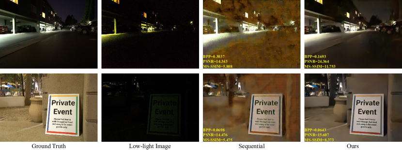
Figure 1: The results of our method compared with the sequential solution show that our method still has a greater advantage in low-light enhancement even at lower bits per pixel (bpp). The sequential solution shown in the figure refers to the compression and then enhancement of low-light images. The example images in the figure are from the SID dataset.

1 Introduction

Lossy image compression, with important applications in media storage and transmission, has been studied for decades. Many traditional image compression standards (e.g., JPEG [56], JPEG2000 [51], BPG [7], and Versatile Video Coding (VVC) [30]) have been proposed, and some of them are widely used in practical applications. In recent years, learning-based image compression methods [13, 22, 64, 57] have developed rapidly and outperformed traditional methods in terms of performance metrics, such as the peak signal-to-noise ratio (PSNR) and the multi-scale structural similarity index (MS-SSIM).

Due to unavoidable environmental influences or technical limitations such as inadequate lighting or the limited exposure time, images are inevitably captured under the influence of sub-optimal lighting conditions (e.g., backlighting, uneven lighting, or dim lighting) [37]. Thus, low-light image enhancement is also widely adopted in many fields, such as visual surveillance and automatic driving. Since existing image compression methods are usually designed for generic natural images, useful information (e.g., texture details), would be severely lost once low-light images are compressed by these methods. However, these information and image details are critical for low-light image enhancement tasks. The enhancement performance would be heavily dropped if they are missing. Based on these considerations, we believe that there is a crucial need for a novel image compression method. It needs to have the capability to preserve useful detail information for low-light enhancement tasks during the compression process, while also having the ability to achieve high compression rates.

The straightforward solution is that the image compression and low-light image enhancement are conducted separately in the sequential order (“Compress before Enhance” or “Enhance before Compress”). However, combining separate models sequentially does not produce optimal results for this joint task. First, the sequential solution introduces additional time costs due to intermediate results, resulting in lower efficiency than the unified approach. Second, error accumulation and loss of information in the individual models plague the sequential solution (see Figure 1). Lossy image compression algorithms are generally not adaptive for low-light images because the loss of useful detail image information after compression can impact low-light image enhancement performance. Under the condition of minimizing the impact on low-light enhancement performance as much as possible, we desire to simultaneously achieve a higher compression rate and better enhancement performance for low-light images. In the image processing field, many researchers have studied joint optimization solutions as an alternative to sequential solutions and have achieved promising results, such as joint image compression and denoising [12], joint image demosaicing and denoising [19], and joint low-light image enhancement and deblurring [80].

In this work, we propose a novel solution to optimize image compression by jointly learning low-light image enhancement. The crucial challenge in solving this joint task is to maintain useful information when compressing low-light images. We design an end-to-end trainable two-branch architecture with the main enhancement branch for obtaining compressed domain features and the signal-to-noise ratio (SNR) aware branch for obtaining local/non-local features. Then, the local/non-local features are fused with the compressed domain features to generate the enhanced features for jointly compressing and enhancing low-light images simultaneously. Finally, the enhanced image is reconstructed by the main decoder. Our proposed joint optimization solution achieves significant advantages compared to sequential solutions, please see Figure 1 for visualization. In summary, the contributions of this work are as follows:

• A joint optimization framework is proposed to achieve the goal of simultaneously earning a higher compression rate and better enhancement performance for low-light images.

• We propose an effective two-branch architecture that has the ability to preserve useful detail information in low-light images while compressing.

• Our proposed joint optimization method achieves outstanding performance while consuming significantly less computational cost than sequential solutions.

2 Related Works

Learning-based lossy image compression.

Learning-based image compression methods have shown great potential, which has led to a growing interest among researchers in this field. Lossy image compression usually contains transform, quantization, and entropy coding.

There are some works that focus on quantization. Works [4, 5] used the additive uniform noise $\mathcal{U}(-0.5,0.5)$ instead of the true quantization during the training. Agustsson et al. [1] proposed soft-to-hard vector quantization to replace scalar quantization. Dumas et al. [16] aimed to learn the quantization step size for each latent feature map.

Some works focus on the transform, e.g., generalized divisive normalization (GDN) [2, 3, 4], residual block [55], attention module [13, 79], non-local attention module [11], attentional multi-scale back projection [18], window attention module [84], stereo attention module [62], and expanded adaptive scaling normalization(EASN) [54] have been used to improve the nonlinear transform. Invertible neural network-based architecture [9, 24, 25, 42, 43, 64] and transformer-based architecture [50, 83, 84] also have been utilized to enhance the modeling capacity of the transforms.

Some other works aim to improve the efficiency of entropy coding, e.g., scale hyperprior entropy model [5], channel-wise entropy model [47], context model [35, 45, 46], 3D-context model [21], multi-scale hyperprior entropy model [26], discretized Gaussian mixture model [13], checkerboard context model [23], split hierarchical variational compression (SHVC) [53], information transformer (Informer) entropy model [32], bi-directional conditional entropy model [36], unevenly grouped space-channel context model (ELIC) [22], neural data-dependent transform [57], multivariate Gaussian mixture model [82]. By constructing more accurate entropy models, these methods have achieved more efficient image compression.

However, these existing learning-based compression methods usually do not consider the impact on low-level image processing tasks (e.g., low-light image enhancement, denoising) when designing. They may cause unwilling performance when combined with image processing tasks.

Learning-based low-light image enhancement.

Many learning-based low-light image enhancement methods [8, 20, 28, 29, 31, 39, 40, 44, 52, 59, 60, 63, 67, 66, 68, 69, 71, 72, 73, 74, 75, 76, 77, 78] have been proposed with compelling success in recent years.

For supervised methods, Zhu et al. [81] proposed a two-stage method called EEMEFN, which comprises muti-exposure fusion and edge enhancement. Xu et al. [66] proposed a frequency-based decomposition-and-enhancement model network. It first learns to recover image contents in a low-frequency layer and then enhances high-frequency details according to recovered contents. Sean et al. [48] introduced three different types of deep local parametric filters to enhance low-light images.

For semi-supervised methods, Yang et al. [70] proposed the semi-supervised deep recursive band network (DRBN) to extract a series of coarse-to-fine band representations of low-light images. The DRBN has been extended by using Long Short Term Memory (LSTM) networks and obtaining better performance [71].

For unsupervised methods, Jiang et al. [28] proposed an unsupervised generative adversarial network (EnlightenGAN) which is the first work that successfully attempts at introducing unpaired training for low-light image enhancement. Ma et al. [44] developed a self-calibrated illumination learning method and defined the unsupervised training loss to improve the generalization ability of the model.

However, when low-light images are compressed, then these low-light enhancement methods usually become very ineffective (shown in Figure 1). In addition, most low-light image enhancement networks have complex structural designs, and their architectures are not suited to combine with image compression directly to achieve joint optimization.

Joint solutions.

A series of individual operations are usually included in image pipeline processing. In conventional schemes, each individual operation is designed and optimized separately, and an error accumulation effect occurs in the pipeline process. The success of joint optimization of multiple tasks using a single network architecture has attracted the attention of researchers with the development of deep learning. In the image process, some works studied for joint optimization have made progress including joint denoising and demosaicing [17, 19], joint image demosaicing, denoising and super-resolution [65], joint low-light enhancement and denoising [41], and joint low-light enhancement and deblurring [80]. Recently, some works [12, 14] optimize image processing and image compression jointly. Cheng et al. [12] jointed image compression and denoising to resolve the bits misallocation problem. Jeong et al. [27] proposed the RAWtoBit network (RBN), which jointly optimizes camera image signal processing and image compression. However, these methods cannot solve the problem of losing useful detail in low-light image compression, which ultimately leads to poor low-light enhancement effects.

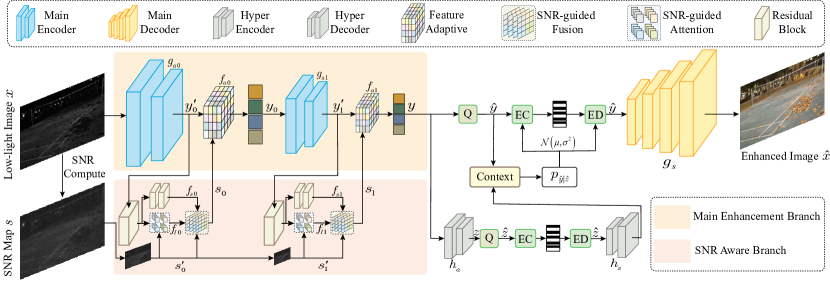
Figure 2: The network architecture of jointly optimizing image compression and low-light enhancement. The left half of the figure contains two branches, the “Main Enhancement Branch” and the “SNR Aware Branch”. The low-light image is fed into the “Main Enhancement Branch” to obtain the two-level enhanced compressed domain features ($y_{0}$/$y$) via “Feature Adaptive” modules ($f_{a0}$/$f_{a1}$). The “SNR Aware Branch” obtains local/non-local information by the SNR-map $s$ and compressed domain features ($y_{0}^{\prime}$/$y_{1}^{\prime}$). The right half of the figure contains the main decoder, entropy models, context model, and hyper encoder/decoder commonly used in recent learning-based compression methods [13, 46]. “/” means “or” in this manuscript.

3 Methodology

3.1 Problem Formulation

Lossy image compression.

This paragraph presents the formulation of the learning-based lossy image compression. In the widely used variational auto-encoder based framework [5], the source image $x$ is transformed to the latent representation $y$ by the parametric encoder $g_{a}(x;\phi_{a})$. The latent representation $y$ is quantized to discrete value $\hat{y}$ which is losslessly encoded to bitstream using entropy coders [15, 61]. During the decoding, $\hat{y}$ is obtained through entropy decoding the bitstream. Finally, $\hat{y}$ is inversely transformed to the reconstructed image $\hat{x}$ through the parametric decoder $g_{s}(\hat{y};\phi_{s})$. In fact, the optimization of the image compression model for the rate-distortion performance can be realized by minimizing the expectation Kullback-Leibler (KL) divergence between intractable true posterior $p_{\hat{y}|x}(\hat{y}|x)$ and parametric variational density $q(\hat{y}|x)$ over the data distribution $p_{x}$ [5]:

$$\mathbb{E}_{x\sim p_{x}}D_{KL}[q(\hat{y}|x)||p({\hat{y}|x})]=\mathbb{E}_{x\sim p_{x}}\mathbb{E}_{\hat{y}\sim q}\bigl{[}\cancelto{0}{\log q(\hat{y}|x)}$$ (1)

$$-\underbrace{\log p_{x|\hat{y}}(x|\hat{y})}_{\text{weighted distortion}}-\underbrace{\log p_{\hat{y}}(\hat{y})}_{\text{rate}}\bigr{]}+\textrm{const},$$

where $D_{KL}[\cdot||\cdot]$ is the KL divergence. Given the transform parameter $\phi_{a}$, the transform $y=g_{a}(x;\phi_{a})$ (from $x$ to $y$) is determined and the process of quantizing $y$ is equivalent to adding uniform distribution $\mathcal{U}(-1/2,1/2)$ for relaxation. Therefore, $q({\hat{y}|x})=\prod_{i}\mathcal{U}(\hat{y}_{i}-1/2,\hat{y}_{i}+1/2)$ and the first term $\log q(\hat{y}|x)=0$. The second term $\log p_{x|\hat{y}}(x|\hat{y})$ is the expected distortion between source image $x$ and reconstructed image $x^{\circ}$. The third term reflects the cost of entropy encoding $\hat{y}$.

In order to make the second term of Eq. 1 easier to calculate. Suppose that the likelihood is give by $p(x|\hat{y})=\mathcal{N}(x|x^{\circ},(\mathfrak{p}\cdot\lambda)^{-1}1)$. In addition, considering the introduction of scale hyperprior. Similar to works [5, 13], the rate-distortion objective function can be written as:

$$\mathbb{E}_{x\sim p_{x}}\mathbb{E}_{\hat{y},\hat{z}\sim q}\bigl{[}\lambda\cdot\left\|x-x^{\circ}\right\|_{\mathfrak{p}}^{\mathfrak{p}}-\log p_{\hat{y}|\hat{z}}(\hat{y}|\hat{z})-\log p_{\hat{z}}(\hat{z})\bigr{]},$$ (2)

where the parameter $\lambda$ is the trade-off between distortion loss and rate loss. If the value of $\mathfrak{p}$ is 2, the first term is the mean square error (MSE) distortion loss. The additional side information $\hat{z}$ is used to capture spatial dependencies.

Learning-based low-light image enhancement.

This paragraph presents the formulation of the learning-based low-light image enhancement problem under the supervised learning-based framework. The low-light image refer as $x\in\mathbb{R}^{3\times h\times w}$ . $h$ and $w$ denote the height and width of the low-light image respectively. The low-light enhancement process is expressed as:

$$\bar{x}=\mathcal{G}(x;\theta),$$ (3)

where the $\bar{x}$ denotes the reconstructed low-light enhancement image. $\theta$ represents the learnable parameters of the neural network $\mathcal{G}$. The optimization of the learning-based low-light image enhancement model is done by minimizing loss to learn the optimal network parameters $\hat{\theta}$:

$$\hat{\theta}=\mathop{\textrm{argmin}}_{\theta}\mathcal{L}_{e}(\mathcal{G}(x;\theta),x^{gt})=\mathop{\textrm{argmin}}_{\theta}\mathcal{L}_{e}(\bar{x},x^{gt}).$$ (4)

The loss function $\mathcal{L}_{e}(\cdot,\cdot)$ usually can use $L_{1}$, $L_{2}$, or Charbonnier [34] loss, etc. The network parameters $\theta$ can be optimized by minimizing the error between the reconstructed image $\bar{x}$ and the ground truth image $x^{gt}$.

Joint optimization.

Based on Eq. 2 and Eq. 4, we further develop the joint optimization formulation of image compression and low-light enhancement. We optimize rate distortion and low-light enhancement jointly as follows:

$$\mathcal{L}= \lambda_{d}\cdot\mathcal{D}(x^{gt},\hat{x})+\mathcal{R}(\hat{y})+\mathcal{R}(\hat{z})$$ (5)

$$= \lambda_{d}\cdot\mathbb{E}_{x\sim p_{x}}\bigl{[}\left\|x^{gt}-\hat{x}\right\|_{\mathfrak{p}}^{\mathfrak{p}}\bigr{]}$$

$$-\mathbb{E}_{\hat{y}\sim q_{\hat{y}}}\bigl{[}\log p_{\hat{y}|\hat{z}}(\hat{y}|\hat{z})\bigr{]}-\mathbb{E}_{\hat{z}\sim q_{\hat{z}}}\bigl{[}\log p_{\hat{z}}(\hat{z})\bigr{]}.$$

The first term $\mathcal{D}(x^{gt},\hat{x})$ measures distortion between the ground truth image $x^{gt}$ and the enhanced image $\hat{x}$. The second term $\mathcal{R}(\hat{y})$ and third term $\mathcal{R}(\hat{z})$ denote the compression levels. $\lambda_{d}$ denotes the weighting coefficient, which is used to balance the trade-off between compression levels and distortion. If $\mathfrak{p}=2$, the first term is the mean square error (MSE) distortion loss.

3.2 Framework

Overall workflow.

Figure 2 shows an overview of the joint optimization framework for image compression and low-light image enhancement. The low-light image $x$ is transformed to the enhanced compressed domain features $y$ by main encoders $g_{a0}$ and $g_{a1}$ with SNR-guided feature adaptive operations. Then $y$ is quantized to the discrete enhanced compressed domain features $\hat{y}$ by the quantizer Q. The uniform noise $\mathcal{U}(-1/2,1/2)$ is added to the enhanced compressed domain features $y$ instead of non-differentiable quantization operation during the training and rounding the enhanced compressed domain features $y$ during testing [5].

We use the hyper-prior scale [5, 46] module to effectively estimate the distribution $p_{\hat{y}|\hat{z}}\sim\mathcal{N}(\mu,\sigma^{2})$ of the discrete enhanced compressed domain features $\hat{y}$ by generating parameters ($\mu$ and $\sigma$) of the Gaussian entropy model to support entropy coding/decoding (EC/ED). The latent representation $z$ is quantized to $\hat{z}$ by the same quantization strategy as the enhanced features $y$. The distribution of latent representation $\hat{z}$ is estimated by the factorized entropy model [4]. The range asymmetric numeral system [15] is used to losslessly compress discrete enhanced features $\hat{y}$ and latent representation $\hat{z}$ into bitstreams. The decoded enhanced features $\hat{y}$ obtained by the entropy decoding are fed into the main decoder $g_{s}$ to reconstruct the enhanced image $\hat{x}$.

Two branch architecture.

Our proposed joint optimization framework includes two branches. The first is the signal-to-noise ratio (SNR) aware branch. The SNR map $s$ is achieved by employing a no-learning-based denoising operation (refer Eq. 6) which is simple yet effective. Local/non-local information on the low-light image is obtained through the SNR-aware branch. The second is the main enhancement branch, the compressed domain features ($y_{0}^{\prime}$/$y_{1}^{\prime}$) combine with the local/non-local information ($s_{0}$/$s_{1}$) generated by the SNR-aware branch to obtain the enhanced compressed domain features ($y_{0}$/$y$).

3.3 Enhanced Compressed Domain Features

As the Figure 2 shows, the SNR map $s\in\mathbb{R}^{h\times w}$ is estimated from the low-light image $x\in\mathbb{R}^{3\times h\times w}$. The calculation process starts by converting low-light image $x$ into grayscale image $\dot{x}\in\mathbb{R}^{h\times w}$ and then proceeds as follows:

$$\ddot{x}=kernel(\dot{x}),\quad n=abs(\dot{x}-\ddot{x}),\quad s=\frac{\ddot{x}}{n},$$ (6)

where $kernel(\cdot)$ denotes averaging local pixel groups operation, $abs(\cdot)$ denotes taking absolute value function.

The SNR map $s$ is processed by the residual block module (“Residual Block” in Figure 2) and transformer-based module (“SNR-guided Attention” in Figure 2) with generating the local features ($f_{s0}$/$f_{s1}$) and the non-local features ($f_{l0}$/$f_{l1}$) inspired by the work [67]. Local and non-local features are fused. It is illustrated in “SNR-guided Fusion” of Figure 2 and is calculated as follows:

$$\begin{split}&s_{0}=f_{s0}\times s_{0}^{\prime}+f_{l0}\times(1-s_{0}^{\prime}),\\ &s_{1}=f_{s1}\times s_{1}^{\prime}+f_{l1}\times(1-s_{1}^{\prime}),\end{split}$$ (7)

where $s_{0}^{\prime}$ and $s_{1}^{\prime}$ are resized from SNR map $s$ according to the shape of corresponding features ($f_{s0}$/$f_{s1}$/$f_{l0}$/$f_{l1}$). $s_{0}$ and $s_{1}$ are SNR-aware fusion features.

Since the SNR map $s$ is unavailable in the decoding process, we consider enhancing the features $y_{0}$ and $y$ in the compressed domain instead of the manner [67] using the decoded domain. Thus, the enhanced image $\hat{x}$ can be obtained by decoding the enhanced features $\hat{y}$ directly. The compressed domain features ($y_{0}^{\prime}$/$y_{1}^{\prime}$) are enhanced by “Feature Adaptation” modules (refered as $f_{a0}$/$f_{a1}$), shown in Figure 2, and their details are shown in Figure 3.

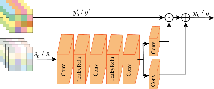
Figure 3: Architecture details of the “Feature Adaptive” module. SNR-aware fusion features ($s_{0}$/$s_{1}$) act as a condition on the compressed domain features ($y_{0}^{\prime}$/$y_{1}^{\prime}$) to generate enhanced features ($y_{0}$/$y$). $\odot$ denotes the Hadamard product and $\oplus$ denotes the addition by element.

3.4 Training Strategy

In our experiments, we observe that training both image compression and low-light image enhancement tasks jointly at the beginning results in convergence problems. Thus, we adopt the two-stage training.

Pre-train without SNR-aware branch.

We pre-train the framework without joining the signal-to-noise ratio (SNR) aware branch. In this case, the network structure is similar to the Cheng2020-anchor [13] of the CompressAI library [6] implementation. The rate-distortion loss is:

$$\mathcal{L}= \lambda_{d}\cdot\mathcal{D}(x,\hat{x})+\mathcal{R}(\hat{y})+\mathcal{R}(\hat{z})$$ (8)

$$= \lambda_{d}\cdot\mathbb{E}_{x\sim p_{x}}\bigl{[}\left\|x-\hat{x}\right\|_{\mathfrak{p}}^{\mathfrak{p}}\bigr{]}$$

$$-\mathbb{E}_{\hat{y}\sim q_{\hat{y}}}\bigl{[}\log p_{\hat{y}|\hat{z}}(\hat{y}|\hat{z})\bigr{]}-\mathbb{E}_{\hat{z}\sim q_{\hat{z}}}\bigl{[}\log p_{\hat{z}}(\hat{z})\bigr{]},$$

where $x$ and $\hat{x}$ denote the original image and decoded image respectively. We set the $\lambda_{d}=0.0016$. It is worth noting that the parameter $\mathfrak{p}$ of the first term $\mathbb{E}_{x\sim p_{x}}\bigl{[}\left\|x-\hat{x}\right\|_{\mathfrak{p}}^{\mathfrak{p}}\bigr{]}$ is equal to 2. That means, the distortion loss $\mathcal{D}(x,\hat{x})$ is the MSE loss instead of $L_{1}$ loss.

Train the entire network.

We train the entire network by loading the pre-trained parameters. The joint optimization loss is Eq. 5. The parameter $\mathfrak{p}$ of the first term $\mathbb{E}_{x\sim p_{x}}\bigl{[}\left\|x^{gt}-\hat{x}\right\|_{\mathfrak{p}}^{\mathfrak{p}}\bigr{]}$ is equal to 1. That means, the distortion loss $\mathcal{D}(x^{gt},\hat{x})$ is $L_{1}$ loss instead of the MSE loss. In our experiment, using $L_{1}$ distortion loss is more beneficial for the stability of training.

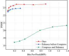
(a) PSNR on SID

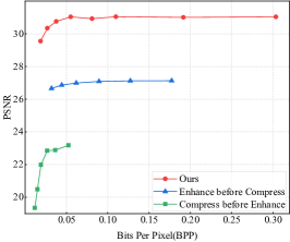
(b) PSNR on SDSD-indoor

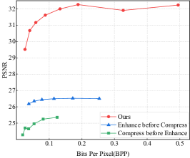
(c) PSNR on SDSD-outdoor

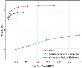
(d) MS-SSIM on SID

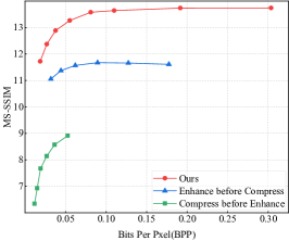
(e) MS-SSIM on SDSD-indoor

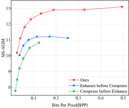
(f) MS-SSIM on SDSD-outdoor

Figure 4: Rate-distortion performance curves aggregated over the SID, SDSD-indoor, and SDSD-outdoor. (a)/(b)/(c) and (d)/(e)/(f) are results on SID, SDSD-indoor, and SDSD-outdoor about PSNR and MS-SSIM, respectively. Remarkably, we are the first to address the problem of error accumulation and information loss in the joint task of image compression and low-light image enhancement, so there is no existing method for comparison. We adopt the state-of-the-art low-light enhancement method [67] for comparison. Experimental results obviously show that our proposed joint optimization method achieves great advantages compared to both “Compress before Enhance” and “Enhance before Compress” sequential solutions.

4 Experiments

4.1 Datasets and Implementation Details

Datasets.

The Flicker 2W [38] is used in the pre-training stage. The low-light datasets that we use include SID [10], and SDSD [58]. The SID contains pairs of short- and long-exposure images with the resolution of $960\times 512$. The SID has heavy noise because they are captured in extreme darkness. The SDSD (static version) contains an indoor subset and an outdoor subset with low-light and normal-light pairs. We set up splitting for training and testing based on the work [67]. All data are converted to the RGB domain for experiments.

Implementation details.

We use the anchor model [13] as our main architecture except for the “Feature Adaptive” modules and the SNR-aware branch. Randomly cropped patches with a resolution of $512\times 512$ pixels are used to optimize the network during the pre-training stage. Our implementation relies on Pytorch [49] and an open-source CompressAI PyTorch library [6]. The networks are optimized using the Adam [33] optimizer with a mini-batch size of 8 for approximately 900000 iterations and trained on RTX 3090 GPUs. The initial learning rate is set as $10^{-4}$ and decayed by a factor of 0.5 at iterations 500000, 600000, 700000, and 850000. The number of pre-training iteration steps is 150000. We have a loss cap for each model, so the network will skip optimizing a mini-step if the training loss is above the specified threshold. We select the same hyperparameters as in Cheng2020-anchor [13] with channel number $\mathrm{N}=128$. We train our model under 8 qualities, where $\lambda_{d}$ is selected from the set {0.0001, 0.0002, 0.0004, 0.0008, 0.0016, 0.0028, 0.0064, 0.012}. To verify the performance of the algorithm, the peak signal-to-noise ratio (PSNR) and the multi-scale structural similarity index (MS-SSIM) are used as evaluation metrics. We also compare the size of the models and computational cost. For better visualization, the MS-SSIM is converted to decibels $(-10log_{10}(1-MS\mbox{-}SSIM))$ as in previous work [13].

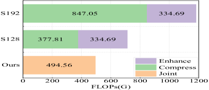
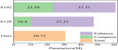
Figure 5: Comparison of computational cost and model size. “S128”/“S192” represents sequential solution that 128/192 channel Cheng2020-anchor method [13] before the low-light image enhancement method Xu2022 [67]. It is obvious that our proposed solution needs far less computational cost and fewer model parameters.

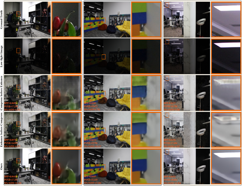
Figure 6: Visualization of comparison results on SDSD-indoor dataset. The comparison of our proposed joint optimization solution with both “Compress before Enhance” and “Enhance before Compress” sequential solutions shows that the low-light image enhancement performance of our method is still more advantageous at lower bits per pixel (bpp). Best viewed in color and zoom in. For more visualization results, please refer to the supplementary material.

4.2 Algorithm Performance

Rate-distortion performance.

Sequential solutions contain individual models of the state-of-the-art low-light image enhancement method Xu2022 [67] and the typical image compression method Cheng2020-anchor [13]. We compare the proposed joint optimization solution with the following sequential solutions: 1) “Compression before Enhance”; 2) “Enhance before Compress”.

For image compression models, we use the pre-trained models (Cheng2020-anchor) provided by CompressAI PyTorch library [6]. For the low-light enhancement method Xu2022, we use the pre-trained models obtained from the official GitHub page to test images. We show the overall rate-distortion (RD) performance curves on SID, SDSD-indoor, and SDSD-outdoor datasets in Figure 4. It can be seen that our proposed solution (red curves) achieves great advantages with common metrics PSNR and MS-SSIM.

The green and blue RD curves indicate that both sequential solutions are worse than our proposed joint solution. Intuitively, the error accumulation and loss of information in the individual models plague the sequential solution. Especially, the compressed low-light images with information loss make it difficult for the low-light image enhancement network to reconstruct pleasing images.

Computational complexity.

We compare the computational cost and model size of the proposed solution with the sequential solution of the typical learning-based image compression method Cheng2020-anchor [13] and the state-of-the-art low-light image enhancement method Xu2022 [67]. As shown in Figure 5, the left side of the figure shows the computational cost over an RGB image with a resolution of $960\times 512$, and the right side of the figure shows the number of model parameters. In our proposed joint solution, the low-light image enhancement and image compression share the same feature extractor during the encoding/decoding. Thus, the proposed joint solution needs far less computational cost and fewer model parameters.

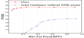
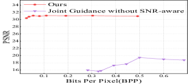
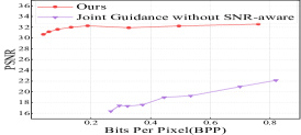
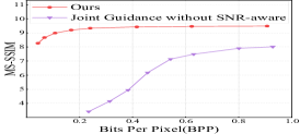
(a) SID

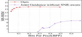
(b) SDSD-indoor

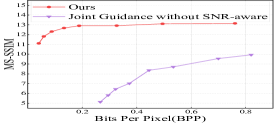
(c) SDSD-outdoor

Figure 7: RD performance curves aggregated over SID, SDSD-indoor, and SDSD-outdoor datasets. It is obvious that our proposed joint method (red curves) achieves great advantages compared to the “Joint Guidance without SNR-aware” method (purple curves), which indicates the effectiveness of the SNR-aware branch.

4.3 Visualization Results

The more visualized comparison results shown in Figure 6 further demonstrate the advantages of our proposed joint optimization solution. These results show that our method can obtain better-quality reconstructed images even with lower bpp. It indicates that our proposed joint optimization solution can indeed solve the problem of the error accumulation and loss of information in the individual models that plague the sequential solution.

4.4 Analysis and Discussion

Impact of the SNR-aware branch.

The SNR-aware branch is able to effectively extract local and non-local information from the low-light image by being aware of the signal-to-noise ratio, which is crucial for our low-light image enhancement. To verify the effectiveness of the SNR-aware branch, we remove the SNR-aware branch and add corresponding network modules to the main enhancement branch to achieve low-light image enhancement. We name this method “Joint Guidance without SNR-aware”. The model architecture is similar to work [12]. More details of this method are given in the supplementary material. Figure 7 shows the results of our method compared with “Joint Guidance without SNR-aware”, which indicates that our proposed method is more effective than “Joint Guidance without SNR-aware”. This method of simply using corresponding network modules in the main enhancement branch is ineffective for the joint optimization of image compression and low-light enhancement tasks.

5 Conclusion

We propose a novel framework to jointly optimize image compression with low-light image enhancement, solving the problem of detail loss when the two tasks are performed in sequential manners. Local and non-local features (obtained by the SNR-aware branch) would be fused with the compressed features to generate enhanced features. The experiments show that the proposed joint optimization framework outperforms sequential methods significantly with fewer computational costs.

References

- [1] Eirikur Agustsson, Fabian Mentzer, Michael Tschannen, Lukas Cavigelli, Radu Timofte, Luca Benini, and Luc V Gool. Soft-to-hard vector quantization for end-to-end learning compressible representations. In NeurIPS, 2017.
- [2] Johannes Ballé, Valero Laparra, and Eero P Simoncelli. Density modeling of images using a generalized normalization transformation. In ICLR, 2016.
- [3] Johannes Ballé, Valero Laparra, and Eero P. Simoncelli. End-to-end optimization of nonlinear transform codes for perceptual quality. In PCS, 2016.
- [4] Johannes Ballé, Valero Laparra, and Eero P Simoncelli. End-to-end optimized image compression. In ICLR, 2017.
- [5] Johannes Ballé, David Minnen, Saurabh Singh, Sung Jin Hwang, and Nick Johnston. Variational image compression with a scale hyperprior. In ICLR, 2018.
- [6] Jean Bégaint, Fabien Racapé, Simon Feltman, and Akshay Pushparaja. Compressai: a pytorch library and evaluation platform for end-to-end compression research. arXiv preprint arXiv:2011.03029, 2020.
- [7] Fabrice Bellard. Bpg image format, 2015.
- [8] Jianrui Cai, Shuhang Gu, and Lei Zhang. Learning a deep single image contrast enhancer from multi-exposure images. IEEE Transactions on Image Processing, 27(4):2049–2062, 2018.
- [9] Shilv Cai, Zhijun Zhang, Liqun Chen, Luxin Yan, Sheng Zhong, and Xu Zou. High-fidelity variable-rate image compression via invertible activation transformation. In ACM MM, 2022.
- [10] Chen Chen, Qifeng Chen, Jia Xu, and Vladlen Koltun. Learning to see in the dark. In CVPR, 2018.
- [11] Tong Chen, Haojie Liu, Zhan Ma, Qiu Shen, Xun Cao, and Yao Wang. End-to-end learnt image compression via non-local attention optimization and improved context modeling. IEEE Transactions on Image Processing, 30:3179–3191, 2021.
- [12] Ka Leong Cheng, Yueqi Xie, and Qifeng Chen. Optimizing image compression via joint learning with denoising. In ECCV, 2022.
- [13] Zhengxue Cheng, Heming Sun, Masaru Takeuchi, and Jiro Katto. Learned image compression with discretized gaussian mixture likelihoods and attention modules. In CVPR, 2020.
- [14] Vinicius Alves de Oliveira, Marie Chabert, Thomas Oberlin, Charly Poulliat, Mickael Bruno, Christophe Latry, Mikael Carlavan, Simon Henrot, Frederic Falzon, and Roberto Camarero. Satellite image compression and denoising with neural networks. IEEE Geoscience and Remote Sensing Letters, 19:1–5, 2022.
- [15] Jarek Duda. Asymmetric numeral systems: Entropy coding combining speed of huffman coding with compression rate of arithmetic coding. arXiv preprint arXiv:1311.2540, 2013.
- [16] Thierry Dumas, Aline Roumy, and Christine Guillemot. Autoencoder based image compression: Can the learning be quantization independent? In ICASSP, 2018.
- [17] Thibaud Ehret, Axel Davy, Pablo Arias, and Gabriele Facciolo. Joint demosaicking and denoising by fine-tuning of bursts of raw images. In ICCV, 2019.
- [18] Ge Gao, Pei You, Rong Pan, Shunyuan Han, Yuanyuan Zhang, Yuchao Dai, and Hojae Lee. Neural image compression via attentional multi-scale back projection and frequency decomposition. In ICCV, 2021.
- [19] Michaël Gharbi, Gaurav Chaurasia, Sylvain Paris, and Frédo Durand. Deep joint demosaicking and denoising. ACM Transactions on Graphics (ToG), 35(6):1–12, 2016.
- [20] Chunle Guo, Chongyi Li, Jichang Guo, Chen Change Loy, Junhui Hou, Sam Kwong, and Runmin Cong. Zero-reference deep curve estimation for low-light image enhancement. In CVPR, 2020.
- [21] Zongyu Guo, Yaojun Wu, Runsen Feng, Zhizheng Zhang, and Zhibo Chen. 3-d context entropy model for improved practical image compression. In CVPRW, 2020.
- [22] Dailan He, Ziming Yang, Weikun Peng, Rui Ma, Hongwei Qin, and Yan Wang. Elic: Efficient learned image compression with unevenly grouped space-channel contextual adaptive coding. In CVPR, 2022.
- [23] Dailan He, Yaoyan Zheng, Baocheng Sun, Yan Wang, and Hongwei Qin. Checkerboard context model for efficient learned image compression. In CVPR, 2021.
- [24] Leonhard Helminger, Abdelaziz Djelouah, Markus Gross, and Christopher Schroers. Lossy image compression with normalizing flows. In ICLRW, 2021.
- [25] Yung-Han Ho, Chih-Chun Chan, Wen-Hsiao Peng, Hsueh-Ming Hang, and Marek Domański. Anfic: Image compression using augmented normalizing flows. IEEE Open Journal of Circuits and Systems, 2:613–626, 2021.
- [26] Yueyu Hu, Wenhan Yang, Zhan Ma, and Jiaying Liu. Learning end-to-end lossy image compression: A benchmark. IEEE Transactions on Pattern Analysis and Machine Intelligence, 44(8):4194–4211, 2022.
- [27] Wooseok Jeong and Seung-Won Jung. Rawtobit: A fully end-to-end camera isp network. In ECCV, 2022.
- [28] Yifan Jiang, Xinyu Gong, Ding Liu, Yu Cheng, Chen Fang, Xiaohui Shen, Jianchao Yang, Pan Zhou, and Zhangyang Wang. Enlightengan: Deep light enhancement without paired supervision. IEEE Transactions on Image Processing, 30:2340–2349, 2021.
- [29] Yeying Jin, Wenhan Yang, and Robby T Tan. Unsupervised night image enhancement: When layer decomposition meets light-effects suppression. In ECCV, 2022.
- [30] Joint Video Experts Team (JVET). Vvc official test model vtm. Accessed on April 5, 2021.
- [31] Hanul Kim, Su-Min Choi, Chang-Su Kim, and Yeong Jun Koh. Representative color transform for image enhancement. In ICCV, 2021.
- [32] Jun-Hyuk Kim, Byeongho Heo, and Jong-Seok Lee. Joint global and local hierarchical priors for learned image compression. In CVPR, 2022.
- [33] Diederik P. Kingma and Jimmy Ba. Adam: A method for stochastic optimization. In ICLR, 2015.
- [34] Wei-Sheng Lai, Jia-Bin Huang, Narendra Ahuja, and Ming-Hsuan Yang. Fast and accurate image super-resolution with deep laplacian pyramid networks. IEEE Transactions on Pattern Analysis and Machine Intelligence, 41(11):2599–2613, 2018.
- [35] Jooyoung Lee, Seunghyun Cho, and Seung-Kwon Beack. Context-adaptive entropy model for end-to-end optimized image compression. In ICLR, 2019.
- [36] Jianjun Lei, Xiangrui Liu, Bo Peng, Dengchao Jin, Wanqing Li, and Jingxiao Gu. Deep stereo image compression via bi-directional coding. In CVPR, 2022.
- [37] Chongyi Li, Chunle Guo, Linghao Han, Jun Jiang, Ming-Ming Cheng, Jinwei Gu, and Chen Change Loy. Low-light image and video enhancement using deep learning: A survey. IEEE Transactions on Pattern Analysis and Machine Intelligence, 44(12):9396–9416, 2022.
- [38] Jiaheng Liu, Guo Lu, Zhihao Hu, and Dong Xu. A unified end-to-end framework for efficient deep image compression. arXiv preprint arXiv:2002.03370, 2020.
- [39] Risheng Liu, Long Ma, Jiaao Zhang, Xin Fan, and Zhongxuan Luo. Retinex-inspired unrolling with cooperative prior architecture search for low-light image enhancement. In CVPR, 2021.
- [40] Kin Gwn Lore, Adedotun Akintayo, and Soumik Sarkar. Llnet: A deep autoencoder approach to natural low-light image enhancement. Pattern Recognition, 61:650–662, 2017.
- [41] Yucheng Lu and Seung-Won Jung. Progressive joint low-light enhancement and noise removal for raw images. IEEE Transactions on Image Processing, 31:2390–2404, 2022.
- [42] Haichuan Ma, Dong Liu, Ruiqin Xiong, and Feng Wu. iwave: Cnn-based wavelet-like transform for image compression. IEEE Transactions on Multimedia, 22(7):1667–1679, 2019.
- [43] Haichuan Ma, Dong Liu, Ning Yan, Houqiang Li, and Feng Wu. End-to-end optimized versatile image compression with wavelet-like transform. IEEE Transactions on Pattern Analysis and Machine Intelligence, 44(3):1247–1263, 2022.
- [44] Long Ma, Tengyu Ma, Risheng Liu, Xin Fan, and Zhongxuan Luo. Toward fast, flexible, and robust low-light image enhancement. In CVPR, 2022.
- [45] Fabian Mentzer, Eirikur Agustsson, Michael Tschannen, Radu Timofte, and Luc Van Gool. Conditional probability models for deep image compression. In CVPR, 2018.
- [46] David Minnen, Johannes Ballé, and George D Toderici. Joint autoregressive and hierarchical priors for learned image compression. In NeurIPS, 2018.
- [47] David Minnen and Saurabh Singh. Channel-wise autoregressive entropy models for learned image compression. In ICIP, 2020.
- [48] Sean Moran, Pierre Marza, Steven McDonagh, Sarah Parisot, and Gregory Slabaugh. Deeplpf: Deep local parametric filters for image enhancement. In CVPR, 2020.
- [49] Adam Paszke, Sam Gross, Francisco Massa, Adam Lerer, James Bradbury, Gregory Chanan, Trevor Killeen, Zeming Lin, Natalia Gimelshein, Luca Antiga, Alban Desmaison, Andreas Kopf, Edward Yang, Zachary DeVito, Martin Raison, Alykhan Tejani, Sasank Chilamkurthy, Benoit Steiner, Lu Fang, Junjie Bai, and Soumith Chintala. Pytorch: An imperative style, high-performance deep learning library. In NeurIPS, 2019.
- [50] Yichen Qian, Ming Lin, Xiuyu Sun, Zhiyu Tan, and Rong Jin. Entroformer: A transformer-based entropy model for learned image compression. In ICLR, 2022.
- [51] Majid Rabbani. Jpeg2000: Image compression fundamentals, standards and practice. Journal of Electronic Imaging, 11(2):286, 2002.
- [52] Wenqi Ren, Sifei Liu, Lin Ma, Qianqian Xu, Xiangyu Xu, Xiaochun Cao, Junping Du, and Ming-Hsuan Yang. Low-light image enhancement via a deep hybrid network. IEEE Transactions on Image Processing, 28(9):4364–4375, 2019.
- [53] Tom Ryder, Chen Zhang, Ning Kang, and Shifeng Zhang. Split hierarchical variational compression. In CVPR, 2022.
- [54] Chajin Shin, Hyeongmin Lee, Hanbin Son, Sangjin Lee, Dogyoon Lee, and Sangyoun Lee. Expanded adaptive scaling normalization for end to end image compression. In ECCV, 2022.
- [55] Lucas Theis, Wenzhe Shi, Andrew Cunningham, and Ferenc Huszár. Lossy image compression with compressive autoencoders. In ICLR, 2017.
- [56] Gregory K Wallace. The jpeg still picture compression standard. IEEE Transactions on Consumer Electronics, 38(1):18–34, 1992.
- [57] Dezhao Wang, Wenhan Yang, Yueyu Hu, and Jiaying Liu. Neural data-dependent transform for learned image compression. In CVPR, 2022.
- [58] Ruixing Wang, Xiaogang Xu, Chi-Wing Fu, Jiangbo Lu, Bei Yu, and Jiaya Jia. Seeing dynamic scene in the dark: A high-quality video dataset with mechatronic alignment. In ICCV, 2021.
- [59] Tao Wang, Yong Li, Jingyang Peng, Yipeng Ma, Xian Wang, Fenglong Song, and Youliang Yan. Real-time image enhancer via learnable spatial-aware 3d lookup tables. In ICCV, 2021.
- [60] Yufei Wang, Renjie Wan, Wenhan Yang, Haoliang Li, Lap-Pui Chau, and Alex Kot. Low-light image enhancement with normalizing flow. In AAAI, 2022.
- [61] Ian H Witten, Radford M Neal, and John G Cleary. Arithmetic coding for data compression. Communications of the ACM, 30(6):520–540, 1987.
- [62] Matthias Wödlinger, Jan Kotera, Jan Xu, and Robert Sablatnig. Sasic: Stereo image compression with latent shifts and stereo attention. In CVPR, 2022.
- [63] Wenhui Wu, Jian Weng, Pingping Zhang, Xu Wang, Wenhan Yang, and Jianmin Jiang. Uretinex-net: Retinex-based deep unfolding network for low-light image enhancement. In CVPR, 2022.
- [64] Yueqi Xie, Ka Leong Cheng, and Qifeng Chen. Enhanced invertible encoding for learned image compression. In ACM MM, 2021.
- [65] Wenzhu Xing and Karen Egiazarian. End-to-end learning for joint image demosaicing, denoising and super-resolution. In CVPR, 2021.
- [66] Ke Xu, Xin Yang, Baocai Yin, and Rynson WH Lau. Learning to restore low-light images via decomposition-and-enhancement. In CVPR, 2020.
- [67] Xiaogang Xu, Ruixing Wang, Chi-Wing Fu, and Jiaya Jia. Snr-aware low-light image enhancement. In CVPR, 2022.
- [68] Jianzhou Yan, Stephen Lin, Sing Bing Kang, and Xiaoou Tang. A learning-to-rank approach for image color enhancement. In CVPR, 2014.
- [69] Zhicheng Yan, Hao Zhang, Baoyuan Wang, Sylvain Paris, and Yizhou Yu. Automatic photo adjustment using deep neural networks. ACM Transactions on Graphics, 35(2):1–15, 2016.
- [70] Wenhan Yang, Shiqi Wang, Yuming Fang, Yue Wang, and Jiaying Liu. From fidelity to perceptual quality: A semi-supervised approach for low-light image enhancement. In CVPR, 2020.
- [71] Wenhan Yang, Shiqi Wang, Yuming Fang, Yue Wang, and Jiaying Liu. Band representation-based semi-supervised low-light image enhancement: Bridging the gap between signal fidelity and perceptual quality. IEEE Transactions on Image Processing, 30:3461–3473, 2021.
- [72] Wenhan Yang, Wenjing Wang, Haofeng Huang, Shiqi Wang, and Jiaying Liu. Sparse gradient regularized deep retinex network for robust low-light image enhancement. IEEE Transactions on Image Processing, 30:2072–2086, 2021.
- [73] Syed Waqas Zamir, Aditya Arora, Salman Khan, Munawar Hayat, Fahad Shahbaz Khan, Ming-Hsuan Yang, and Ling Shao. Learning enriched features for real image restoration and enhancement. In ECCV, 2020.
- [74] Hui Zeng, Jianrui Cai, Lida Li, Zisheng Cao, and Lei Zhang. Learning image-adaptive 3d lookup tables for high performance photo enhancement in real-time. IEEE Transactions on Pattern Analysis and Machine Intelligence, 2020.
- [75] Yonghua Zhang, Xiaojie Guo, Jiayi Ma, Wei Liu, and Jiawan Zhang. Beyond brightening low-light images. International Journal of Computer Vision, 129(4):1013–1037, 2021.
- [76] Zhao Zhang, Huan Zheng, Richang Hong, Mingliang Xu, Shuicheng Yan, and Meng Wang. Deep color consistent network for low-light image enhancement. In CVPR, 2022.
- [77] Lin Zhao, Shao-Ping Lu, Tao Chen, Zhenglu Yang, and Ariel Shamir. Deep symmetric network for underexposed image enhancement with recurrent attentional learning. In ICCV, 2021.
- [78] Chuanjun Zheng, Daming Shi, and Wentian Shi. Adaptive unfolding total variation network for low-light image enhancement. In ICCV, 2021.
- [79] Lei Zhou, Zhenhong Sun, Xiangji Wu, and Junmin Wu. End-to-end optimized image compression with attention mechanism. In CVPRW, 2019.
- [80] Shangchen Zhou, Chongyi Li, and Chen Change Loy. Lednet: Joint low-light enhancement and deblurring in the dark. In ECCV, 2022.
- [81] Minfeng Zhu, Pingbo Pan, Wei Chen, and Yi Yang. Eemefn: Low-light image enhancement via edge-enhanced multi-exposure fusion network. In AAAI, 2020.
- [82] Xiaosu Zhu, Jingkuan Song, Lianli Gao, Feng Zheng, and Heng Tao Shen. Unified multivariate gaussian mixture for efficient neural image compression. In CVPR, 2022.
- [83] Yinhao Zhu, Yang Yang, and Taco Cohen. Transformer-based transform coding. In ICLR, 2022.
- [84] Renjie Zou, Chunfeng Song, and Zhaoxiang Zhang. The devil is in the details: Window-based attention for image compression. In CVPR, 2022.