Estimating Class Separability of Datasets Using Persistent Homology with Application to LLM Fine-Tuning

Abstract

This paper proposes a method to estimate the class separability of an unlabeled text dataset by inspecting the topological characteristics of sentence-transformer embeddings of the text. Experiments conducted involve both binary and multi-class cases, with balanced and imbalanced scenarios. The results demonstrate a clear correlation and a better consistency between the proposed method and other separability and classification metrics, such as Thornton’s method and the AUC score of a logistic regression classifier, as well as unsupervised methods. Finally, we empirically show that the proposed method can be part of a stopping criterion for fine-tuning language-model classifiers. By monitoring the class separability of the embedding space after each training iteration, we can detect when the training process stops improving the separability of the embeddings without using additional labels.

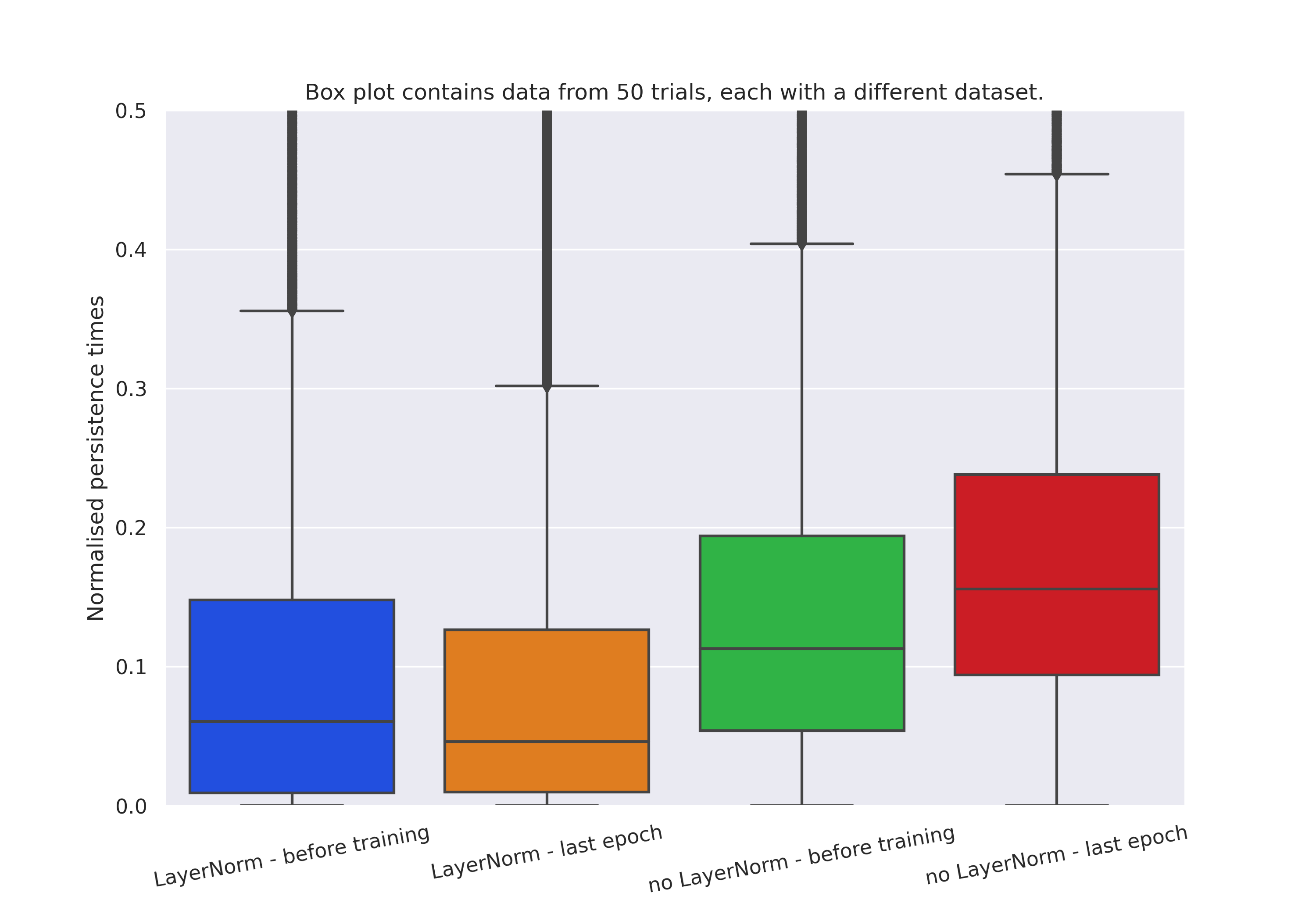
Figure 1: Boxplot of the persistence times of features from the $H_{0}$ group of the embeddings before training and at the final epoch $t=100$ for the toy example in Section 4.1 and $50$ different sample datasets. The persistence times depend on the diameter of the data, so we normalised them by the maximum persistence to account for this. The $H_{0}$ group captures connected components for the underlying manifold. Data with only a few large persistence times tend to be more clustered. In the experiment from Section 4.1, we can see that for the same datasets, a model with a LayerNorm tends to provide topologically-simpler embeddings whereas one without produces embeddings with larger persistence times on average during training. Both models reach the same average performance with respect to AUC (about 0.97) over the fifty datasets.

1 Introduction

Pre-trained language models, having undergone extensive preliminary training, have demonstrated remarkable versatility. They have shown the capacity to generalize to new tasks from a mere handful of examples by employing techniques such as in-context few-shot learning (Brown et al.,, 2020), parameter-efficient fine-tuning (PEFT) (Liu et al.,, 2022), and pattern-exploiting training (Schick and Schütze, 2020a, ). Commonly, these methodologies necessitate the use of language models that vary in size from a few hundred million (Lan et al.,, 2019; Schick and Schütze, 2020b, ) to billions of parameters, exemplified by GPT-3 (Brown et al.,, 2020) and T0 (Sanh et al.,, 2021). Furthermore, these techniques often involve the conversion of a task, such as classification, into a language modeling format, akin to a cloze question.

Embedding data is a crucial part of any language model that maps texts to numerical feature vectors that can be fed to downstream machine learning operations aimed at performing specific tasks, e.g., text classification. Texts with similar meanings need to be mapped to feature vectors closely spaced in the embedding space, while texts with largely distinct meanings need to be mapped further away from each other. If the pre-trained language model is used for text classification, metrics capturing class-separability can be used to assess how good or bad a text embedding is performing. In this case, a good embedding process would generate an embedding manifold with high class-separability so that a downstream classification process would perform well.

In classification problems, class-separability metrics capture how easily features distinguish their corresponding classes (Fukunaga,, 2013). The intuition for adopting these metrics for feature ranking is that we expect good features to embed objects of the same class close to each other in the feature space, while objects of different classes are embedded far away from each other. This can measure the discriminative power of a feature (Rajoub,, 2020). Having those metrics can also assist with capturing the minimum complexity of a decision function for a specific problem, e.g., VC-dimension (Vapnik,, 1998). Typically separability metrics range from model-specific, aka. “wrapper” methods, for example, Gini importance, to more generic “filter” methods that capture intrinsic properties of the data independently of a classifier, e.g., mutual information. A simple such metric is Fisher’s discriminant ratio which quantifies linear separability of data by using the mean and standard deviation of each class (Li and Wang,, 2014). This metric comes with strong assumptions of normality. Geometrically-inspired methods (Greene,, 2001; Zighed et al.,, 2002; Guan and Loew,, 2022; Gilad-Bachrach et al.,, 2004) look at the distances and neighborhoods of features to give a model-independent view of how well-separated the classes are. However, high-dimensional settings and/or large datasets can be challenging for most separability metrics. Most information-theoretic estimators do not scale well with data size or require training separate models (Belghazi et al.,, 2018). Geometric methods are attractive as they are not tied to a classifier, but can be informative only for specific separation regimes (Mthembu and Marwala,, 2008) and are impacted by the complexity of computing graph neighborhoods and distances between the points. Moreover, a common requirement for these class-separability metrics is that they require labeled data, making them mainly limited to the supervised learning setting.

In mathematics, homology is a general way of associating a sequence of algebraic objects, such as abelian groups, with other mathematical objects, such as topological spaces, e.g., data manifolds (Hatcher,, 2002). The fundamental groups of topological spaces, introduced by Poincaré (Munkres,, 2018), are the first and simplest homotopy groups (Hatcher,, 2002) and are algebraic invariants that are critically important for characterizing and classifying topological spaces (Massey,, 1991).

Topological data analysis (TDA) is a mathematical framework that uses topological concepts to analyze and understand complex data sets. TDA is increasingly being used in machine learning to extract information from high-dimensional data that is insensitive to the choice of metric, allowing for more robust analysis. TDA also provides dimensionality reduction and robustness to noise (Carlsson,, 2009). One of the most important techniques in TDA is persistent homology (Malott and Wilsey,, 2019), which is a method for analyzing the topological features of a data set across different scales. Persistent homology tracks the birth and death of topological features, such as connected components, loops, voids, and identifies those that persist across different scales. This approach provides a more nuanced understanding of the underlying structure of the data and allows for clustering and data analysis.

1.1 Related Work

Hajij and Istvan, (2021) framed the classification problem in machine learning by expressing it in topological terms. Using this topological framework, they showed the circumstances under which the classification problem is achievable in the context of neural networks. While we do not make direct use of the formalism, some of our experiments are motivated by the discussion in this work.

Rieck et al., (2019) developed a complexity measure for deep neural networks, called ”neural persistence”, using algebraic topology. This measure was used as stopping criterion that shortens the training process while achieving comparable accuracies as early stopping based on validation loss by taking into account the layers and weights of the whole model. Pérez-Fernández et al., (2021) represented neural networks as abstract simplicial complex, analyzing them using their topological ’fingerprints’ via Persistent Homology (PH). They then described a PH-based representation proposed for characterizing and measuring similarity of neural networks. Experiments demonstrated the effectiveness of this representation as a descriptor of different architectures in several datasets. While there are similarities with our work, we do not use persistent homology to compare different models. Instead, we explicitly focus on examples from classification and only use information from the $H_{0}$ group of the embeddings we get from our model to assess separability.

Gutiérrez-Fandiño et al., (2021) suggested studying the training of neural networks with Algebraic Topology, specifically Persistent Homology. Using simplicial complex representations of neural networks, they studied the Persistent Homology diagram distance evolution on the neural network learning process with different architectures and several datasets. Results showed that the Persistent Homology diagram distance between consecutive neural network states correlates with the validation accuracy, implying that the generalization error of a neural network could be intrinsically estimated without any holdout set. While we are also interested in getting some signal about validation performance, our approach uses only the simplest topological information from the embeddings, $H_{0}$, instead of explicitly taking into account the weights and connections of the whole model. We also track not just statistics of death times, but also their overall density as epochs progress.

Griffin et al., (2023) showed that the topological structure of training data can have a dramatic effect on the ability of a deep neural network (DNN) classifier to learn to classify data. Previously Naitzat et al., (2020) highlighted that DNN tend to simplify the topology of input as it gets passed through the DNN’s layers. Both of those works are connected to ours through the tracking of changes in the topology of embeddings during training and how that affects the performance of the DNN.

1.2 Contributions

Major contributions of the paper are summarised below:

• An unsupervised method for class-separability estimation: We leverage information from the 0-homology groups of data manifolds to extract information on class-separability. Unlike standard supervised techniques, which require labels for computing class-separability, the proposed method can estimate class-separability without requiring labels. Experimental validation conducted in this paper on synthetic and realistic public data shows a clear consistency between the class-separability metric computed by the proposed method and class-separability metric computed by supervised methods such as Thornton’s method and the ROC-AUC score of a logistic regression classifier. The experiments also involve a comparison to an unsupervised method, called Calinski-Harabasz (CH), which demonstrates that the proposed method is more consistent with the supervised methods than the CH.

• Experimental analysis of LLMs embeddings on $H_{0}(X)$ density space: The paper involves experimental analysis of embedding manifold evolution over training epochs based on the densities of $H_{0}(X)$ persistence times. This is accomplished by generating a density $f_{n}$ of $H_{0}(X)$ persistence times of the embedding manifold generated by each training epoch. Then, a sequence of training epochs would give rise to a sequence of densities $\{f_{n}\}$ whose behavior and convergence can be used to estimate class-separability of the data manifold.

1.3 Organization

The paper is organised in six sections, including the present section. Section 2 provides a brief introduction to homology groups and persistent homology of data manifolds. This information is crucial background for understanding the proposed method for estimating class separability of datasets, presented in Section 3 along with the baseline metrics in Section 3.1. Section 3 also describes a semi-supervised paradigm for fine-tuning LLMs with automated stopping criterion based on class separability of embedding manifold estimated using the proposed method. Three sets of experiments for validating the proposed methodology are presented in Section 4. Section 5 discusses the limitations in our method and current study. Finally, Section 6 summarizes and concludes the paper along with recommendations for future research.

2 Background on Persistent Homology

We now briefly introduce the essential notation and concepts of persistent homology that we will use in this work. For more details, please see the supplementary material or Section 2 from Naitzat et al., (2020).

Suppose we have a collection of points $X=\{x_{1}\ldots,x_{N}\}\subset\mathbb{R}^{d}$ and a norm $\|.\|:\mathbb{R}^{d}\times\mathbb{R}^{d}\rightarrow\mathbb{R}$. At a high level, persistent homology (PH) concerns itself with identifying the shape and topological features of data manifolds in a way that is robust to noise.

To be able to identify those, we can start with a standard construction in PH, the Vietoris-Rips  set at scale $\epsilon$:

$$\mathrm{VR}_{\epsilon}(X):=\{\sigma\subset X:\sigma\neq\emptyset,\forall x,y\in\sigma,\|x-y\|\leq\epsilon\}.$$ (1)

For two elements to belong to the same $\sigma$, their $\epsilon$-balls need to intersect. Thus $\mathrm{VR}_{\epsilon}(X)$ generates a filtration, called Vietoris-Rips filtration, on the normed space $(X,\|.\|)$, where $\mathrm{VR}_{0}=\{\{x\}:x\in X\}$ and $\mathrm{VR}_{\infty}=\{x_{1},\ldots,x_{N}\}$.

In PH, the Vietoris-Rips set is called an abstract simplicial complex. If we interpret every $\sigma\in\mathrm{VR}_{\epsilon}$ as describing a relationship between the points $x\in\sigma$, we can construct a geometric realization of $\mathrm{VR}_{\epsilon}(X)$ by building a graph with vertices the points in $X$ and edges described by the relationships in $\mathrm{VR}_{\epsilon}(X)$.

With the techniques of homology and linear algebra, we can assign to a simplicial complex $K_{\epsilon}:=\mathrm{VR}_{\epsilon}(X)$ a set of groups, called the homology groups, $H_{k}(K_{\epsilon})$. These groups describe topological features, the connected components and $k$-dimensional holes for $k\leq d$.

One thing that is special about $\mathrm{VR}_{\epsilon}(X)$ is that $\epsilon$ can be chosen such that the Vietoris-Rips is homotopy-equivalent to the manifold from which $X$ comes from; see Proposition 3.1 in Niyogi et al., (2008) for more details on how $\epsilon$ can be appropriately chosen to ensure the homotopy-equivalence property. In other words, descriptions of the topology of the right $\mathrm{VR}_{\epsilon}$ translate to the topology of the original manifold.

Everything described thus far is standard simplicial homology. However, when applied to noisy real data (represented as point clouds), small differences in the distance between points could imply a large difference in terms of the topology. To account for this, PH considers the Vietoris-Rips filtration, $\{K_{\epsilon}:\epsilon\geq 0\}$. As $\epsilon$ grows, the topology of $K_{\epsilon}$ changes as a result of increasing the radius of every ball in Equation 1. For example, connected components that appeared at scale $\epsilon=\epsilon_{2}$ (birth time) may merge into one component at scale $\epsilon_{5}>\epsilon_{2}$ (death time). PH tracks those changes as $\epsilon$ increases from $0$ to infinity, providing the birth and death time for topological features as well as their total number at each scale.

We call the difference between the death time and the birth time of a topological feature the persistence time of the feature. Features with large persistence times tend to be the most topologically important. In this work, we only concern ourselves with the persistence times of the connected components (i.e., corresponding to $H_{0}$) which we get from the ripser Python library (Tralie et al.,, 2018).

For the remainder of this manuscript and given a dataset $X\subset\mathbb{R}^{d}$, ripser will provide an array of persistence times, $p_{i}$, $i=0,\ldots,M$, one for each connected component discovered. Because persistence times can grow with the diameter of $X$, $\mathrm{diam}(X)=\max_{x,y}\|x-y\|$, we normalise them to $[0,1]$ after removing the special persistence time $p_{M}=\infty$ at $\epsilon=\infty$.

3 Class Separability of Datasets

3.1 Baseline measures of separability

In this section, we briefly describe the measures we will use as proxies for separability. These measures will be used later as baselines in the experiments.

ROC-AUC: An estimate of the area under the ROC curve for logistic regression models trained on labeled data. In the experiments, we estimate the ROC-AUC over different numbers of validation-data splits; we denote this by ROC-AUC-$n$, where $n$ is how many splits we use. In the plots where ROC-AUC-$n$ appears, we plot its mean and $95\%$ confidence intervals.

Thornton Index (Greene,, 2001): The Thornton index is the probability that a random data point’s label is the same as that of each of the nearest neighbors. We estimate it by using its five nearest neighbors.

Both ROC-AUC and Thornton index require an additional set of labeled data. For an unsupervised baseline for separability, we use the Calinski-Harabasz Index.

Calinski-Harabasz Index (CH) (Caliński and Harabasz,, 1974): The CH is often used to measure clustering performance, e.g., of $k$-means. With $k$ clusters and $N$ data points, the index is proportional to $\text{SS}_{B}/\text{SS}_{W}$, where $\text{SS}_{B}$ is the between-cluster variance and $\text{SS}_{W}$ is the within-cluster variance. The larger the CH, the more well-defined the clusters are. CH is implemented for labelled data in scikit-learn, but we instead use k-means with $k=5$ to assign data points to clusters.

While the first two metrics are bounded, CH is not, so it can be difficult to compare them. To help with comparisons, in the experiments we normalize all metrics of separability so their maximum value is equal to one.

3.2 Using persistent homology to capture separability

The proposed method for estimating class separability of a dataset $X$ is solely based on the persistence times of the 0-homology group of the data manifold, $H_{0}(X)$. We argue (and will explore experimentally) that tracking the evolution of the distribution of persistence times can provide information on how a classification model organises its embedding space as well as whether we are getting diminishing returns by further training.

In order to compare the information from the persistence times with the baseline measures from Section 3.1, we need to use an appropriate statistic. We will make two assumptions:

1. Topologically-simpler embedding spaces result in easier classification problems: This is a reasonable assumption that is supported by similar work referenced in Section 1.1.

2. During classification training, models tend to simplify their embedding space.: This assumption does not always hold (as we discuss in the Limitations Section 5). However, we can empirically verify this by tracking the evolution of the densities of the persistence times (compare Figure 8 with Figure 6).

With those assumptions in place, we chose to use $P(\text{persistence}<t)$ as the statistic, where $t$ is a user-defined threshold in $[0,1]$ (but see also the limitations of this statistic in Section 5).

4 Experiments

In this section, we will first start with a synthetic toy example to showcase the behavior of persistence times of the $H_{0}$ group during training. Then, we will proceed to a realistic binary and a subsequent multi-class text example with pre-trained sentence transformers classifiers. In those examples we will see similar behaviors to the toy case and demonstrate how we can use the convergence of the $H_{0}$ persistence times as a proxy for separability.

4.1 Toy Classification Experiment

In this experiment, we want to inspect the topological behavior of embeddings in a toy experiment and as the embedding model is trained in a classification. We will empirically see that a simple feedforward neural network simplifies its embeddings during training based on whether a LayerNorm has been applied or not.

Dataset: The dataset $D$ is generated by scikit-learn’s “make_classification()” and consists of $2000$ $40$-dimensional points with binary labels. The split between the classes is equal. We set the class separation parameter to $0.3$. We provide the complete set of options for this dataset in the supplementary material.

Model: The model used is a fully-connected neural network with two-hidden layers with ReLU activation functions. The first layer has twenty hidden units and the second layer five. The final output of the model is a two-element softmax representing the probability of each class. This model is trained with cross-entropy loss and the Adam optimizer with learning rate 1e-2. For the purposes of this experiment, we construct two such models with PyTorch, $M_{1}$ and $M_{2}$. $M_{1}$ contains a LayerNorm after the second layer. Because we are interested in the behavior of the embeddings through training and not in getting the best possible model, we do not perform a hyperparameter search. We train $M_{1}$ and $M_{2}$ on $1000$ examples of $D$ for $100$ epochs. For each epoch $t$, we embed the $1000$ remaining examples to a five-dimensional space by using the second hidden layer of the models; we will denote these embeddings by $e_{t}$. Then, using ripser, we compute the persistence of the $H_{0}$ features for every $e_{t}$.

While both $M_{1}$ and $M_{2}$ achieved similar results in terms of ROC-AUC for this toy problem, their embeddings exhibit different topological structure according to $H_{0}$; see Figure 1. $M_{1}$, containing the LayerNorm, simplifies further its embedding space whereas $M_{2}$ turns it more topologically diverse. In addition, we notice two distinct behaviors during training (see Figure 2), with the histogram of the persistence times converging to the same shape as early as epoch $40$ with small changes after that.

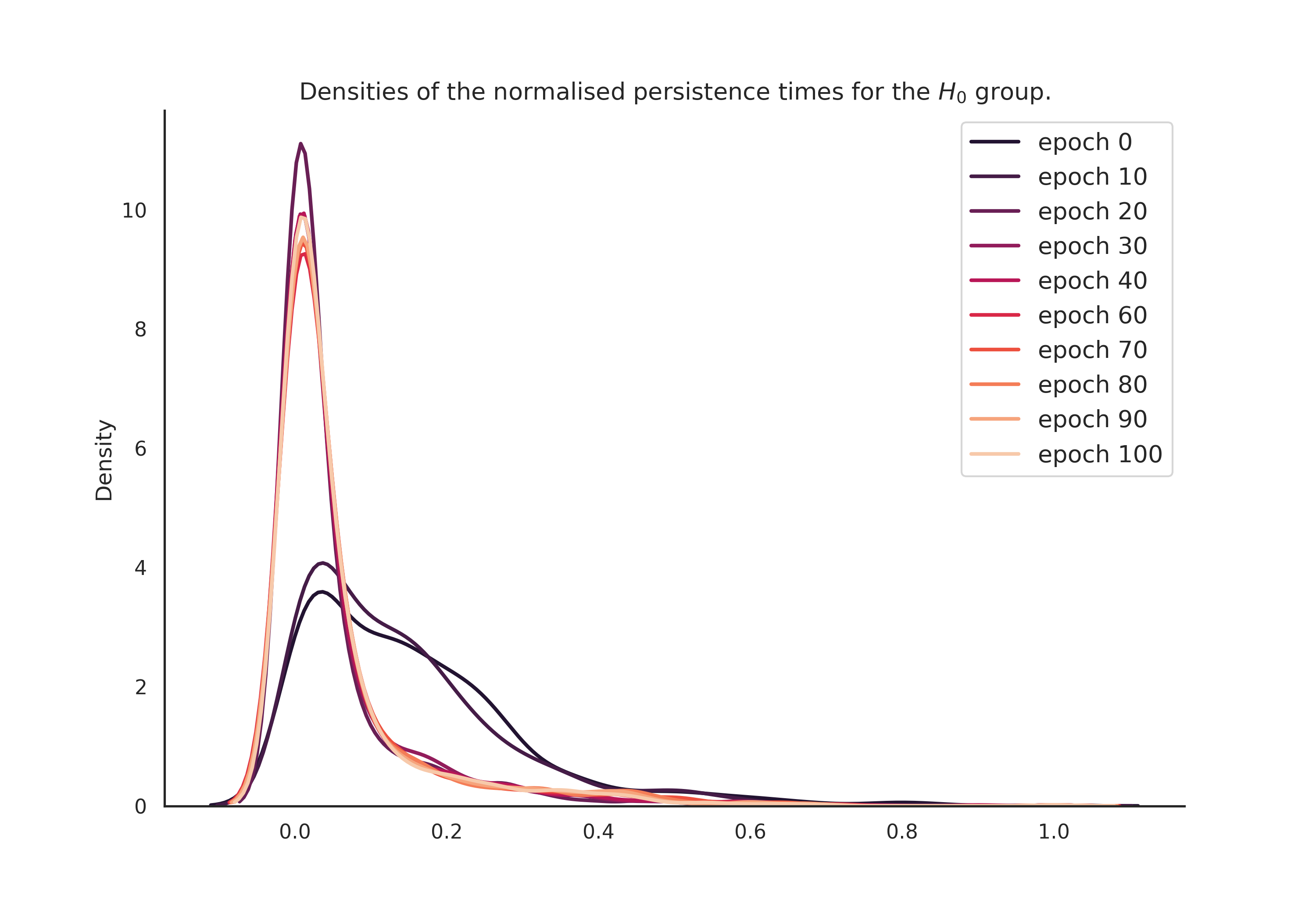
Figure 2: Convergence of the distribution of normalised persistence times of $H_{0}$ for $e_{t}$ as $t:=\text{epochs}\to 100$ for $M_{1}$ (which contains the LayerNorm and is defined as described in Section 4.1). We note that there are two distinct behaviors for epochs less than $30$ and epochs greater than $30$, with the shape of the density seeing little change after epoch $40$. During training, the model simplifies its embedding space (topologically speaking, so most persistence times are approximately $0$, except for the most important ones for the task).

4.2 Binary-Class Text Classification

In this experiment, the setup is similar to Section 4.1, except we will now start from a pre-trained sentence transformer and a realistic binary-classification dataset.

Dataset: We use the train split of the binary-class “SetFit / amazon_counterfactual” dataset from Hugging Face. This dataset contains text from English, German, and Japanese, as well as a label for whether the text is describing a counterfactual or not-counterfactual statement. Only 19% of the text describes counterfactuals. Full details about the split are in the supplementary material. We split this set to a training set with 1000 examples and a tracking set with 1000 examples.

Model: We consider a pre-trained sentence transformer available on Hugging Face and through the sentence-transformers library (Reimers and Gurevych,, 2019). The model is the all-MiniLM-L6-v2 (MiniLM), a popular model for embedding text and constructing text classifiers. It is a six-layer network outputting 384-dimensional sentence embeddings. We attach a randomly-initialised softmax head to turn it into a classifier model. We then train it with Adam, learning rate $1e-5$, cross-entropy loss, and batch size $32$. Similarly to Section 4.1, we train the model with the training set and, first before fine-tuning and then after each epoch, we embed the tracking set examples so that we can study the evolution of their embeddings later.

We remind here that for comparison purposes all of the separability metrics are normalised so that their maximum value is 1 (as the CH is unbounded, see Section 3.1). Figure 3 shows the evolution of the various metrics of separability on the tracking set. The model never sees the labels of this set during training. We observe that the model gradually improves the separability of its embeddings as epochs progress. The CH metric, that captures how well-defined the clusters are, lags behind the rest and has its biggest jump at the fourth epoch. Our proposed metric catches up earlier and, more importantly, changes more slowly as the benefit of additional epochs lessens.

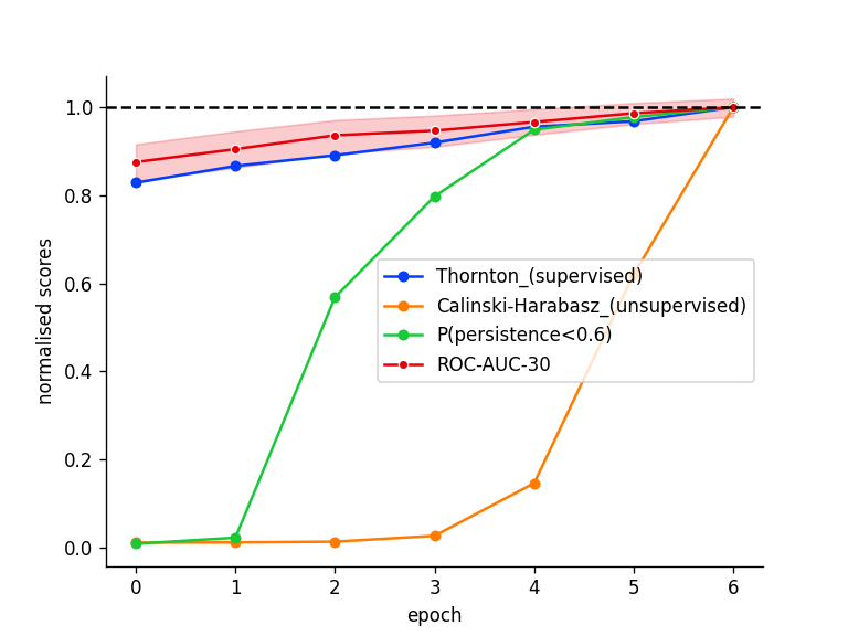
Figure 3: Separability metrics for the binary classification text example with the MiniLM model. The supervised metrics agree from early on and our proposed metric catches up soon after, indicating the benefit of training longer but also potentially stopping at the fourth epoch. The unsupervised CH registers no difference in the first few epochs and only agrees with the final result because it is an increasing function (all scores are normalised so that they take their maximum value is equal to 1).

4.3 Multi-Class Text Classification

In this experiment, we consider the behavior of pre-trained sentence transformers during fine-tuning for multi-class classification. The setup is similar to the binary class experiment in Section 4.2.

Dataset: We use the train split of the multi-class ”SetFit/emotion” dataset from Hugging Face. This dataset contains six classes (with approximate corresponding appearance in the set): “joy” (33.5%), “sadness” (29.1%), “anger” (13.5%), “fear” (12.1%), “love” (8.1%), and “surprise” (3.6%).

Model: In this example, we will use two different sentence transformers. Those are the all-MiniLM-L6-v2 (which we used before) and, for contrast, the paraphrase-albert-small-v2 (albert). This is also a six-layer network that outputs 768-dimensional sentence embeddings. We attach to each of them a randomly-initialised softmax head to turn them into classifier models. The training and tracking setup are the same as in Section 4.2.

Similarly to Section 4.1, we also track $P(p<t)$, the percentage of (normalised) persistence times that are smaller than the threshold $t=0.6$. The results can be seen in Figure 7 and Figure 8.

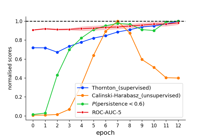
Figure 4: Evolution of various metrics of separability as epochs progress for MiniLM in the multi-class setting. We can see that the supervised metrics, ROC-AUC-5 and Thornton are converging to their maximum values. CH starts decreasing after a while, which is not consistent with the Thornton and ROC-AUC assessment. The probability of persistence stays consistent and the difference between consecutive values gets smaller, indicating convergence.

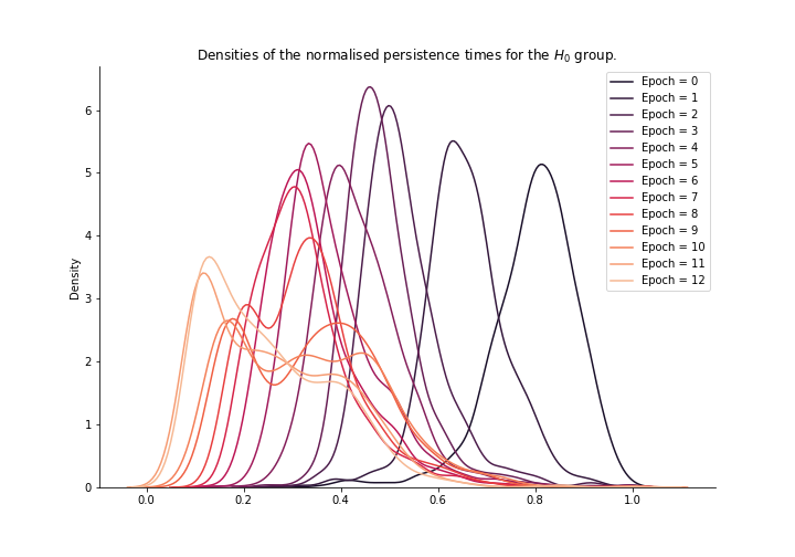
Figure 5: Evolution of the densities of the persistence times for the MiniLM model and the multi-class setting. We can see the topological simplification of the embedding space during training as well as a few distinct states, e.g., the unimodal distribution of persistence times becoming bimodal close to convergence. This bimodality could imply that some components are important for the task and cannot be simplified any further (similarly to the tail in the toy example, see Figure 2).

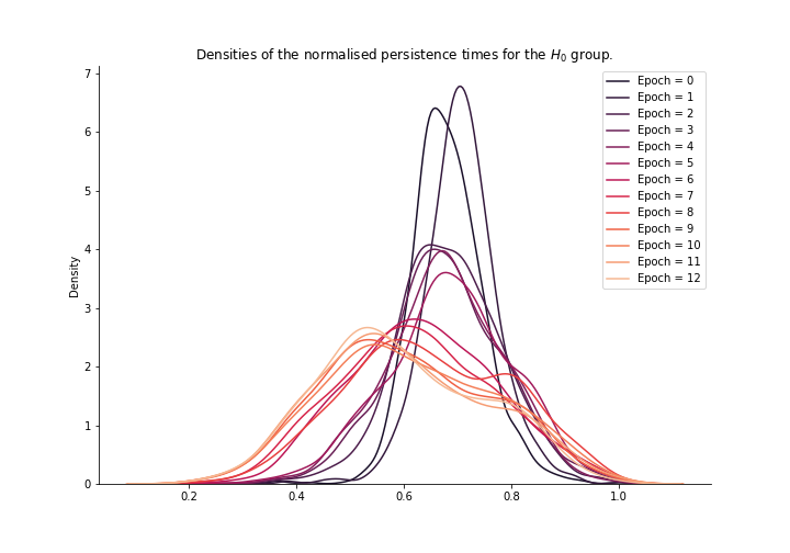
Figure 6: Evolution of the densities of the persistence times for the albert model and the multi-class setting. We can see similar behavior as in the non-LayerNorm example in Section 4.1 with the original persistence times being widened during training as well as distinct phases during fine-tuning. Compare with the behavior in Figure 8. This model got a final AUC of $0.74$, similarly to the MiniLM model. Although this does not provide sufficient evidence for the LayerNorm playing the biggest role in the difference in behavior, we do note that the paraphrase model contains a fully-connected neural network after the last LayerNorm whereas the MiniLM contains a LayerNorm at the end of all layers; see also the supplementary material.

5 Limitations

Computational complexity of $H_{0}$ computations: Methods and algorithms for computing persistent homology of datasets is a rapidly evolving area, where new algorithms and software implementations are being updated and released at a rapid pace (Otter et al.,, 2017). In this paper, we use the ripser library for computing the persistent homology of datasets. It is based on the concept of Vietoris-Rips complexes, which are a way to construct a topological space from a finite set of points (Bauer,, 2021). This method has a run time complexity of $O(2^{n})$, where $n$ is the dataset size, but constant with data dimension, which makes this method preferable for high-dimensional manifolds (Somasundaram et al.,, 2021).

Selection of the summary statistics: While we hope that we have shown the usefulness of tracking the distribution of the persistence times, we do not make a claim that $P(p<t)$ is the optimal statistic to use to summarise the distribution. We plan to elucidate this point formally in future work as well as use higher order information from $H_{k}$ for $k>0$.

Behavior of persistence times during training: While the persistence times of the embedding manifold do not use additional label information explicitly for their calculation, they do depend on the training labels, the model architecture, and the training objective. A lot of our discussion assumed that the model will tend to simplify the topology of their embedding space, at least as far as $H_{0}$ is concerned. We have shown examples where this does not happen, e.g., Figure 6 and Figure 1, and drew a potential explanation of this behavior based on the LayerNorm. While we can check this assumption experimentally by tracking the evolution of the histograms of the persistence times, we are also planning to draw formal connections to architecture in future work.

6 Conclusion

This paper proposes an unsupervised method for estimating class separability of datasets by using topological characteristics of the data manifold. This could be particularly useful when labeled data is limited, as we can get a sense of the improvement of separability as well as diminishing returns on further training from using unlabelled data. Tracking statistics of $H_{0}$ could form part of a fine-tuning methodology of LLMs for text classification, where labeled samples are used for fine-tuning shots while unlabeled data are used for monitoring class separability of the embedding manifold after each fine-tuning shot. Experiments implemented in this paper on different scenarios of balanced and unbalanced data, as well as binary and multi-class classification cases, demonstrate consistency of the class separability estimated by the proposed method, which does not require labels, with supervised methods that do require labels.

Potential topics for future work involve:

• Formalizing the selection of the summary statistic and how that depends on the architecture of the model we train.

• A methodology for training classifiers, e.g. via Pareto optimization, that jointly optimizes a supervised loss that requires labels (e.g., cross-entropy) and an unsupervised loss generated by unlabeled data by the proposed method.

• Expanding the analysis to the densities of persistence times of higher homology groups $H_{n}$ of data manifold and their relations to class-separability of the dataset.

• Expanding the study to tasks outside classification, e.g., regression, text generations, etc.

Disclaimer

This paper was prepared for informational purposes by the Applied Innovation of AI (AI2) and Global Technology Applied Research center of JPMorgan Chase & Co. This paper is not a product of the Research Department of JPMorgan Chase & Co. or its affiliates. Neither JPMorgan Chase & Co. nor any of its affiliates makes any explicit or implied representation or warranty and none of them accept any liability in connection with this paper, including, without limitation, with respect to the completeness, accuracy, or reliability of the information contained herein and the potential legal, compliance, tax, or accounting effects thereof. This document is not intended as investment research or investment advice, or as a recommendation, offer, or solicitation for the purchase or sale of any security, financial instrument, financial product or service, or to be used in any way for evaluating the merits of participating in any transaction.

Appendix A Details on Models

A.1 Toy example

This subsection provides the python code for producing the model used to generate results involved in Sec. 4.1 in the main manuscript.

import torch

class Net(torch.nn.Module):
    def __init__(self, input_units, middle_layer_units=20, use_layer_norm=False):
        super(Net, self).__init__()
        self.fc1 = torch.nn.Linear(input_units, 20)
        self.fc2 = torch.nn.Linear(20, middle_layer_units)
        self.fc3 = torch.nn.Linear(middle_layer_units, 2)
        self.use_layer_norm = use_layer_norm

        if use_layer_norm:
            self.layer_norm = torch.nn.LayerNorm(middle_layer_units)

        self.relu = torch.nn.ReLU()
        self.softmax = torch.nn.Softmax(dim=1)

    def hidden_layers(self, x):
        x = self.fc1(x)
        x = self.relu(x)
        x = self.fc2(x)
        x = self.relu(x)
        return self.layer_norm(x) if self.use_layer_norm else x

    def forward(self, x):
        x = self.hidden_layers(x)
        x = self.softmax(self.fc3(x))
        return x

    def encode(self, x):
        x = self.hidden_layers(x)
        return x.detach().numpy()

A.2 Binary and Multi-Class text experiment

This subsection provides the python code for producing the model used to generate the results involved in Sec. 4.2 in the main manuscript. Specifically, to load a sentence-transformer and turn it into a classifier model, we use:

import torch.nn as nn
from sentence_transformers import SentenceTransformer

class STClassifier(nn.Module):
    """
    Simple implementation of a sentence-transformer classifier.
    """

    def __init__(self, model: SentenceTransformer, device: str = "gpu", n_class: int = 1):
        super(STClassifier, self).__init__()

        self.model = model.to(device)

        for param in self.model.parameters():
            param.requires_grad = True

        if n_class == 1:
            self.classifier = nn.Sequential(
                nn.Linear(self.model.get_sentence_embedding_dimension(), 1),
                nn.Sigmoid(),
            ).to(device)
        else:
            self.classifier = nn.Sequential(
                nn.Linear(self.model.get_sentence_embedding_dimension(), n_class),
                nn.Softmax(dim=1),
            ).to(device)

        self.device = device

    def forward(self, x):
        x = {
            key: value.to(self.device) for key, value in self.model.tokenize(x).items()
        }
        x = self.model(x)["sentence_embedding"].to(self.device)
        x = self.classifier(x)
        return x

    def encode(self, x):
        return self.model.encode(x, convert_to_tensor=True)


model_name = "all-MiniLM-L6-v2"
DEVICE = "cpu"

st_model = SentenceTransformer(model_name, device=DEVICE)
classifier = STClassifier(st_model, device=DEVICE)

The training options per experiment, e.g., learning rate, optimizer, etc., are described in the main text.

Appendix B Details on experiments

B.1 Toy Experiment

B.1.1 Boxplot

To construct the boxplot, we consider $50$ datasets consecutively generated with the make_classification() method using the following settings:

from sklearn import datasets

X, y = datasets.make_classification(
        n_classes=2,
        n_samples=2000,
        n_features=40,
        n_redundant=0,
        n_informative=40,
        n_clusters_per_class=np.random.randint(1,4),
        class_sep=0.5,
        hypercube=True,
        shuffle=True
        )

This generates a random dataset at each call. We further randomise the number of clusters per class between $1$ and $4$ and set the argument class_sep as $0.5$ to ensure that the dataset is not trivially linearly-separable. Each dataset is split to two halves, one for training and one for tracking.

For each dataset, we train one model using a LayerNorm and one without a LayerNorm as described in the main manuscript.

B.1.2 Density plot

Parameters and code used to generate the dataset for the toy example:

N_FEAT = 40
from sklearn import datasets
    X,y = datasets.make_classification(
    n_classes=2,
    n_samples=2000,
    n_features=N_FEAT,
    n_redundant=0,
    n_informative=N_FEAT,
    n_clusters_per_class=1,
    random_state=0,
    class_sep=0.3,
)

B.2 Binary-Class Text Experiment

To load the data used for this experiment, we used the following snippet:

from datasets import load_dataset
dataset = load_dataset("SetFit/amazon_counterfactual", split="train")

train_dataset = dataset.select(range(1000))
test_dataset = dataset.select(range(1000, 3000))
data_to_embed = test_dataset.shuffle(42).select(range(1000))

As described in the main manuscript, we embed data_to_embed before training and after every epoch with the sentence transformer’s encode() method so that we can study the evolution of the embeddings at the end.

B.3 Multi-Class Text Experiment

B.3.1 Data loading

To load the data for this experiment, we used the following snippet:

from datasets import load_dataset

dataset = load_dataset("SetFit/emotion", split="train")

# split into train and test
train_dataset = dataset.select(range(1000))
test_dataset = dataset.select(range(1000, 3000))
data_to_embed = test_dataset.shuffle(42).select(range(1000))

As described in the main manuscript, we embed data_to_embed before training and after every epoch with the sentence transformer’s encode() method so that we can study the evolution of the embeddings at the end.

B.3.2 Calculation of the ROC-AUC for the multi-class case

For the multi-class case, we are calculating the ROC-AUC by using the scikit-learn function “roc_auc_score” with the “multi_class” parameter set to “one-vs-one”. This option is more stable towards class-imbalance (as also documented in the “roc_auc_score” documentation page: https://scikit-learn.org/stable/modules/generated/sklearn.metrics.roc_auc_score.html).

Appendix C Details on pre-trained sentence-transformer models

For both text classification experiments, the fine-tuning process used a single Tesla T4 GPU with 16GB of RAM.

C.1 all-MiniLM-L6-v2

The all-MiniLM-L6-v2 (MiniLM) is a six layer pre-trained sentence-transformer. To conserve space, we limit the printout below to the important elements. MiniLM begins as:

0.auto_model.embeddings
0.auto_model.embeddings.word_embeddings
0.auto_model.embeddings.position_embeddings
0.auto_model.embeddings.token_type_embeddings
0.auto_model.embeddings.LayerNorm
0.auto_model.embeddings.dropout
0.auto_model.encoder.layer.0.attention.self.dropout
0.auto_model.encoder.layer.0.attention.output.dense
0.auto_model.encoder.layer.0.attention.output.LayerNorm
0.auto_model.encoder.layer.0.attention.output.dropout
0.auto_model.encoder.layer.0.intermediate.dense
0.auto_model.encoder.layer.0.output.dense
0.auto_model.encoder.layer.0.output.LayerNorm
0.auto_model.encoder.layer.0.output.dropout

The $0$ layer is then repeated five more times until we get to a pooler layer:

0.auto_model.pooler
0.auto_model.pooler.dense
0.auto_model.pooler.activation

We can see that there is a LayerNorm after each dense layer.

C.2 sentence-transformers/paraphrase-albert-small-v2

The sentence-transformers/paraphrase-albert-small-v2 (albert) is a six-layer pre-trained sentence transformer based on albert-small-v2: https://huggingface.co/nreimers/albert-small-v2.

albert’s composition is as follows:

    SentenceTransformer(
  (0): Transformer({
    ’max_seq_length’: 100,
    ’do_lower_case’: False
  }) with Transformer model: AlbertModel
  (1): Pooling({
    ’word_embedding_dimension’: 768,
    ’pooling_mode_cls_token’: False,
    ’pooling_mode_mean_tokens’: True,
    ’pooling_mode_max_tokens’: False,
    ’pooling_mode_mean_sqrt_len_tokens’: False
    })
)

If we look deeper within the architecture, we get:

0.auto_model.embeddings.word_embeddings
0.auto_model.embeddings.position_embeddings
0.auto_model.embeddings.token_type_embeddings
0.auto_model.embeddings.LayerNorm
0.auto_model.embeddings.dropout
0.auto_model.encoder
0.auto_model.encoder.embedding_hidden_mapping_in
0.auto_model.encoder.albert_layer_groups
0.auto_model.encoder.albert_layer_groups.0
0.auto_model.encoder.albert_layer_groups.0.albert_layers
0.auto_model.encoder.albert_layer_groups.0.albert_layers.0
0.auto_model.encoder.albert_layer_groups.0.albert_layers.0.full_layer_layer_norm
0.auto_model.encoder.albert_layer_groups.0.albert_layers.0.attention
0.auto_model.encoder.albert_layer_groups.0.albert_layers.0.attention.query
0.auto_model.encoder.albert_layer_groups.0.albert_layers.0.attention.key
0.auto_model.encoder.albert_layer_groups.0.albert_layers.0.attention.value
0.auto_model.encoder.albert_layer_groups.0.albert_layers.0.attention.attention_dropout
0.auto_model.encoder.albert_layer_groups.0.albert_layers.0.attention.output_dropout
0.auto_model.encoder.albert_layer_groups.0.albert_layers.0.attention.dense
0.auto_model.encoder.albert_layer_groups.0.albert_layers.0.attention.LayerNorm
0.auto_model.encoder.albert_layer_groups.0.albert_layers.0.ffn
0.auto_model.encoder.albert_layer_groups.0.albert_layers.0.ffn_output
0.auto_model.encoder.albert_layer_groups.0.albert_layers.0.activation
0.auto_model.encoder.albert_layer_groups.0.albert_layers.0.dropout
0.auto_model.pooler
0.auto_model.pooler_activation

We note that there is a fully-connected layer after the last LayerNorm.

Appendix D Detailed background of persistent homology

This subsection provides a brief introduction to simplicial homology and persistent homology of data manifolds, which form the backbone of the proposed method for estimating class separability of datasets, presented in the next section. While the details are given in standard literature on algebraic topology Hatcher, (2002); Munkres, (2018), the essential concepts are presented below for the completeness of this paper.

D.1 Simplicial homology

Simplicial homology is a fundamental tool in algebraic topology that captures the topological features of a simplicial complex Fugacci et al., (2016). It associates a sequence of abelian groups called homology groups to a simplicial complex, which provides information about the connected components, holes, and higher-dimensional voids in the complex.

A $p$-simplex is a geometric object that serves as a building block for constructing spaces, such as points (0-simplices), edges (1-simplices), triangles (2-simplices), tetrahedra (3-simplices), and so on. Formally, a $p$-simplex is defined as the convex hull of $(p+1)$ affinely independent points in Euclidean space. The vertices of a simplex are often referred to as its face.

A simplicial complex $\mathcal{K}$ is a finite set of simplices such that $\sigma\in\mathcal{K}$ and $\tau\leq\sigma$ implies $\tau\in\mathcal{K}$, and the intersection of any two simplices of $\mathcal{K}$ is either empty or a face of both simplices Matoušek, (2003). A simplicial complex serves as a combinatorial representation of a topological space, and its homology groups can be used to study the topological features of the space.

Given a simplicial complex $\mathcal{K}$, we can construct the $p$-th chain group $C_{p}$ of $\mathcal{K}$, which consists of all combinations of $p$-simplices in $\mathcal{K}$. For instance, let $\mathcal{K}=\{\{a\},\{b\},\{c\},\{a,b\},\{b,c\},\{a,c\}\}$. We can list valid simplicial $1$-chains of $\mathcal{K}$ as follows: $\{a,b\}$, $\{b,c\}$, $\{a,c\}$, $\{a,b\}+\{a,c\}$, $\{a,c\}+\{b,c\}$, $\{a,b\}+\{b,c\}$, $\{a,b\}+\{b,c\}+\{a,c\}$. This allows us to define the $p$-th boundary operator $\partial_{p}:C_{p}(\mathcal{K})\rightarrow C_{p-1}(\mathcal{K})$ as the homomorphism that assigns each simplex $\sigma=\{v_{0},\dots,v_{p}\}\in\mathcal{K}$ to its boundary:

$$\partial_{p}(\sigma):=\sum_{i=0}^{p}(-1)^{i}\{v_{0},\dots,\widehat{v_{i}},\dots,v_{p}\},$$ (2)

where $\{v_{0},\dots,\widehat{v_{i}},\dots,v_{p}\}$ is the $i^{th}$ face of $\sigma$ obtained by deleting $i^{th}$ vertex. Boundaries do not have a boundary themselves, hence $\partial_{p-1}\circ\partial_{p}=0$ for all $p$. For example, let $\sigma$ be a solid triangle with vertices $a$, $b$, and $c$. Then $\partial_{2}(\sigma)=ab+bc+ca$. The boundary of any edge $xy$ is $y-x$. So, $\partial_{1}(\partial_{2}(\sigma))=b-a+c-b+a-c=0$.

Given a simplicial complex $\mathcal{K}$, we can construct a chain complex, which is a sequence of abelian groups $C_{0},C_{1},\dots,C_{n}$ connected by boundary operators $\partial_{p}$:

$$0\xrightarrow[]{\partial_{n+1}}C_{n}\xrightarrow[]{\partial_{n}}C_{n-1}\xrightarrow[]{\partial_{n-1}}\dots\xrightarrow[]{\partial_{2}}C_{1}\xrightarrow[]{\partial_{1}}C_{0}\xrightarrow[]{\partial_{0}}0.$$ (3)

The $p$-th homology groups of $\mathcal{K}$, denoted $H_{p}(\mathcal{K})$, is defined as the quotient abelian group:

$$H_{p}:=Z_{p}/B_{p},$$ (4)

where $Z_{p}:=\ker(\partial_{p})$ is the cycle group, and $B_{p}:=\mathrm{im}(\partial_{p+1})$ is the boundary group.

Given the homology groups, we can extract a crucial collection of topological invariants known as the Betti numbers. The $p$-th Betti number, $\beta_{p}$, is determined as the rank of the corresponding $p$-th homology group, expressed as $\beta_{p}=\textrm{rank}(H_{p})$. Intuitively, $\beta_{0}$ indicates the number of connected components, $\beta_{1}$ the number of “holes” or loops, $\beta_{2}$ the number of cavities, and so forth.

D.2 Persistent homology

Persistent homology is a powerful tool in topological data analysis that quantifies the multiscale topological features of a filtered simplicial complex Carlsson, (2009). It captures the birth and death of topological features such as connected components, holes, and higher-dimensional voids as the threshold parameter varies.

Let $X=\{x_{1},\dots,x_{n}\}$ be a set of points (dataset) and $d$ be a metric, such as the Euclidean distance. For a chosen threshold parameter $\epsilon$, the Vietoris-Rips complex $\mathcal{V}_{\epsilon}$ is defined as:

$$\mathcal{V}_{\epsilon}:=\{\sigma\subseteq X\mid\forall u,v\in\sigma:d(u,v)\leq\epsilon\}.$$ (5)

A filtration of $\mathcal{V}_{\epsilon}$ is a nested collection of subcomplexes $\mathcal{V}=\{\mathcal{V}_{\epsilon}:\epsilon\in[0,\infty)\}$ that can be used to track the evolution of homology groups as the simplicial complex is built up incrementally. For $i\leq j$, the $p$-th persistent homology group, denoted by $H_{p}^{i,j}$, captures the homology classes of $\mathcal{K}_{i}$ that persist in $\mathcal{K}_{j}$ and is defined as:

$$H_{p}^{i,j}:=Z_{p}(\mathcal{K}_{i})/(B_{p}(\mathcal{K}_{j})\cap Z_{p}(\mathcal{K}_{i})).$$ (6)

We associate each homology class $\alpha\in H_{p}(\mathcal{K}_{i})$ with a birth time $b$ and a death time $d$ Malott and Wilsey, (2019). The birth time of $\alpha$ is the smallest value of $i$ for which $\alpha\in H_{p}(\mathcal{K}_{i})$ but $\alpha\notin H_{p}^{i-1,i}$. The death time is the smallest index $j\geq i$ for which $\alpha$ is no longer in $H_{p}(F_{j})$ (i.e., $\alpha$ is merged with another class or becomes a boundary). The persistence of $\alpha$ is the difference between its death and birth times, $d-b$. This difference captures the significance of the homology class in the complex.

These results are represented by persistence diagrams, which are scatterplots of points in the plane that encode the birth and death of topological features. Each point $(b,d)$ in the persistence diagram corresponds to a topological feature (e.g., a connected component or a hole) that is born at filtration step $b$ and dies at step $d$. The persistence diagrams provide a visual representation of the significance and lifespan of topological features.

Appendix E Additional Experiments

E.1 Multi-Class Experiment on SetFit/20_newsgroups dataset

Dataset: We use the train split of the multi-class SetFit/20_newsgroups dataset from Hugging Face. This dataset contains twenty classes with approximately equal number of examples each. It is loaded in the same way as the SetFit/emotion dataset.

Model: We consider two pre-trained sentence transformers, both available on Hugging Face and through the sentence-transformers library. Those are the all-MiniLM-L6-v2 and paraphrase-albert-small-v2. Both are six-layer networks outputting 384 and 768 dimensional sentence embeddings respectively. We attach to each of them a randomly initialised softmax layer to turn them into classifier models $S_{2}$ and $S_{1}$. Both are trained with Adam with learning rate $1e-5$ and cross-entropy loss. We train the models on the same $1000$ examples and embed a different set of $1000$ examples at each epoch so that we can inspect their topology at the end. We train each model for ten epochs.

Similarly to the main text, we track $P(\text{persistence times}<t)$, that is the percentage of (normalised) persistence times that are smaller than the threshold $t=0.6$. The results can be seen in Figure 7 and Figure 8.

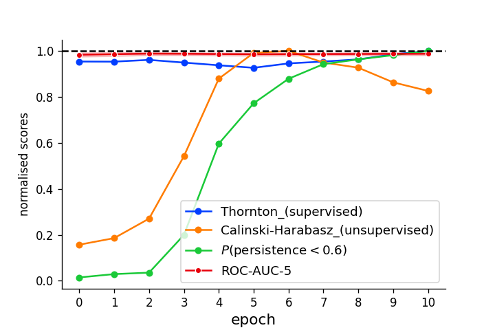
Figure 7: Evolution of various metrics of separability as epochs progress. We can see that the supervised metrics, ROC-AUC-5 (that is, ROC-AUC estimated over 5 splits), and Thornton are converging to their maximum values. CH starts decreasing after a while, which is not consistent with the Thornton assessment. The probability of persistence stays consistent and gets each maximum value at the same time with the supervised metrics.

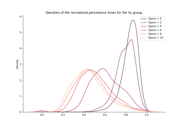
Figure 8: Evolution of the densities of the persistence times for the Mini-LM model and the multi-class setting. We can see similarities to the results in the main text: convergence of the densities, simplification of the topological space, as well as distinct states during training.

References

- Bauer, (2021) Bauer, U. (2021). Ripser: efficient computation of Vietoris-Rips persistence barcodes. J. Appl. Comput. Topol., 5(3):391–423.
- Belghazi et al., (2018) Belghazi, M. I., Baratin, A., Rajeshwar, S., Ozair, S., Bengio, Y., Courville, A., and Hjelm, D. (2018). Mutual information neural estimation. In International conference on machine learning, pages 531–540. PMLR.
- Brown et al., (2020) Brown, T., Mann, B., Ryder, N., Subbiah, M., Kaplan, J. D., Dhariwal, P., Neelakantan, A., Shyam, P., Sastry, G., Askell, A., et al. (2020). Language models are few-shot learners. Advances in neural information processing systems, 33:1877–1901.
- Caliński and Harabasz, (1974) Caliński, T. and Harabasz, J. (1974). A dendrite method for cluster analysis. Communications in Statistics-theory and Methods, 3(1):1–27.
- Carlsson, (2009) Carlsson, G. (2009). Topology and data. Bulletin of The American Mathematical Society - BULL AMER MATH SOC, 46:255–308.
- Fugacci et al., (2016) Fugacci, U., Scaramuccia, S., Iuricich, F., and Floriani, L. D. (2016). Persistent Homology: a Step-by-step Introduction for Newcomers. In Pintore, G. and Stanco, F., editors, Smart Tools and Apps for Graphics - Eurographics Italian Chapter Conference. The Eurographics Association.
- Fukunaga, (2013) Fukunaga, K. (2013). Introduction to Statistical Pattern Recognition. Computer science and scientific computing. Elsevier Science.
- Gilad-Bachrach et al., (2004) Gilad-Bachrach, R., Navot, A., and Tishby, N. (2004). Margin based feature selection-theory and algorithms. In Proceedings of the twenty-first international conference on Machine learning, page 43.
- Greene, (2001) Greene, J. (2001). Feature subset selection using thornton’s separability index and its applicability to a number of sparse proximity-based classifiers. In Proceedings of annual symposium of the pattern recognition association of South Africa.
- Griffin et al., (2023) Griffin, C., Karn, T., and Apple, B. (2023). Topological structure is predictive of deep neural network success in learning.
- Guan and Loew, (2022) Guan, S. and Loew, M. (2022). A novel intrinsic measure of data separability. Applied Intelligence, pages 1–17.