Generative AI for Bayesian Computation

Abstract

Generative AI (Gen-AI) methods are developed for Bayesian Computation. Gen-AI naturally applies to Bayesian models which can be easily simulated. First, we generate a large training dataset of data and parameters from the joint probability model. Secondly, we find a summary/sufficient statistic for dimensionality reduction. Thirdly, we use a deep neural network to uncover the inverse Bayes map between parameters and data. This finds the inverse posterior cumulative distribution function. Bayesian computation then is equivalent to high dimensional regression with dimensionality reduction (a.k.a feature selection) and nonlnearity (a.k.a. deep learning). The main advantage of Gen-AI is the ability to be density-free and hence avoids MCMC simulation of the posterior. Architecture design is important and we propose deep quantile NNs as a general framework for inference and decision making. To illustrate our methodology, we provide three examples: a stylized synthetic example, a traffic flow prediction problem and a satellite data-set. Finally, we conclude with directions for future research.

1 Introduction

Our goal is to develop Generative AI for Bayesian Computation. The main goal of Bayesian computation is to calculate the posterior distribution $p(\theta\mid y)$ from a likelihood function, $p(y\mid\theta)$ or forward model $y=f(\theta)$ and prior distribution $p(\theta)$. This is notoriously hard for high-dimensional models. Generative AI directly learns the inverse posterior mapping from parameters $\theta$ to data $y$. The main advantage of generative AI is that it is density-free and thus doesn’t rely on the use of iterative simulation methods such as MCMC or Particle filters.

Specifically, Gen-AI starts with a large sample from a joint distribution of observables and parameters $(y^{(i)},\theta^{(i)})\sim p(y,\theta)$ for $1\leq i\leq N$. The inverse Bayes map is simply given by the multivariate inverse CDF. We write $\theta=F^{-1}_{\theta\mid y}(\tau)$, where $\tau$ is a vector of standard uniforms. Given a training data set $(y^{(i)},\theta^{(i)},\tau^{(i)})_{i=1}^{N}$, we train the map $\theta^{(i)}=H\left(S\left(y^{(i)}\right),\tau^{(i)}\right)$, where $S$ is a fixed dimension sufficient statistic and $H$ is a deep neural network. Designing the NN architecture for $H$ is the main challenge in any applied problem. We then evaluate the learned map evaluated at the observed $y_{\mathrm{obs}}$ and a new $\tau$. Namely, the posterior inference is summarized by $\theta\stackrel{{\scriptstyle D}}{{=}}H(S(y_{\mathrm{obs}}),\tau)\;\;{\rm where}\;\;\tau\sim U(0,1)$. Deep Quantile NNs provide a general framework for training $H$ and for decision making whilst providing an alternative to invertible NN approaches such as normalizing flows.

To learn an inverse CDF (quantile function) $F^{-1}(\tau,y)=f_{\psi,\phi}(\tau,y)$, we use a kernel embedding trick and augment the predictor space. We then use the quantile function to generate samples from the target distribution. We represent the quantile function is a function of superposition for two other functions $F^{-1}(\tau,y)=f_{\psi,\phi}(\tau,y)=g(\psi(y)\circ\phi(\tau))$ where $\circ$ is the element-wise multiplication operator. Both functions $g$ and $\phi$ are feed-forward neural networks. To avoid over-fitting, we use a sufficiently large training dataset. This architecture was shown to work well a reinforcement learning context (Dabney et al.,, 2018).

Traditional methods such as MCMC directly simulate from the posterior density. Whereas generative AI uses deep neural networks to directly model the parameters, given the data, as a nonlinear map. This map depends on a fixed dimensional sufficient statistic and a randomly generated uniform error. From von Neumann decomposition, the mapping is the inverse posterior CDF. Put simply, generative AI solves the central problem of Bayesian computation which is learning a high-dimensional mapping/projection in random variable parameter space. Quantile deep neural networks and their ReLu/$\tanh$ counterparts provide a natural architecture. Approximation properties of those networks are discussed in Polson and Ročková, (2018). Dimensionality reduction can be performed using auto-encoders and partial least-squares (Polson et al.,, 2021) due to the result by Brillinger, (2012); Bhadra et al., (2021), see survey by Blum et al., (2013) and kernel embeddings approach discussed by Park et al., (2016). Generative AI circumvents the need for methods like MCMC that require the density evaluations.

Generative AI requires the researcher to learn the dimensionality-reduced summary/sufficient statistics, along with a non-linear map (Jiang et al.,, 2017; Albert et al.,, 2022). A useful interpretation of the sufficient statistic as a posterior mean, which also allows us to view posterior inputs as one of the inputs to the posterior mean. One can also view a NN is an approximate nonlinear Bayes filter to perform such tasks (Müller et al.,, 1997). Our framework provides a natural link for black box methods and stochastic methods, as commonly known in the machine learning literature (Bhadra et al.,, 2021; Breiman,, 2001). Our work builds on Jiang et al., (2017) who were the first to propose deep learners for dimension reduction methods and to provide asymptotic theoretical results. Our approach also builds on the insight by Dabney et al., (2018); Ostrovski et al., (2018) that implicit quantile neural networks can be ued to approximated posterior distributions that arise in decision theory. Dabney et al., (2017) also show the connection between the widely used Wasserstein distance and quantile function.

ABC methods can be viewed as a variation of this approach, where $H$ is learned via nearest neighbors. Jiang et al., (2017) show that a natural choice of $S$ is via the posterior mean. Papamakarios and Murray, (2016) shows how to use mixture density networks (Bishop,, 1994) to approximate the posterior for ABC calculations. For a discussion of the ABC framework for a parametric exponential family, see Beaumont et al., (2002) and Nunes and Balding, (2010) for the optimal choice of summary statistics. A local smoothing version of ABC is given in Jiang et al., (2018); Bernton et al., (2019) Fearnhead and Prangle, (2012), Longstaff and Schwartz, (2001) take a basis function approach. Pastorello et al., (2003) provide an estimation procedure when latent variables are present.

For low-dimensional $\theta$, the most simple approach is to discretize the parameter space and the data space and use a lookup table to approximate $p(\theta\mid y)$. This is the approach taken by Jiang et al., (2017). However, this approach is not scalable to high-dimensional $\theta$. For practical cases, when the dimension of $\theta$ is high, we can use conditional independence structure present in the data to decompose the joint distribution into a product of lower-dimensional functions (Papamakarios et al.,, 2017). In machine learning literature a few approaches were proposed that rely on such a decomposition (van den Oord and Kalchbrenner,, 2016; Germain et al.,, 2015; Papamakarios et al.,, 2017). Most of those approaches use KL divergence as a metric of closeness between the target distribution and the learned distribution.

A natural approach to model posterior distribution using a neural network is to assume that parameters of a neural network are random variables to use either approximation or MCMC techniques to model the posterior distribution over the parameters (Izmailov et al.,, 2021). A slightly different approach is to assume that only weights of the last output layer of a neural network are stochastic (Wang et al.,, 2022; Schultz et al.,, 2022).

The rest of the paper is outlined as follows. Section 1.1 provides a review of the existing literature. Sections 2 and 3 describes our GenAI-Bayes Bayesian algorithm. Sections 4 provides two applications. To illustrate our methodology, we provide three examples: a stylized synthetic example, a traffic flow prediction problem and a satellite data-set. Finally, Section 5 concludes with directions for future research.

1.1 Connections with Previous Work

Although deep learning have been widely used in engineering (Polson and Sokolov,, 2017; Dixon et al.,, 2019; Polson and Sokolov,, 2017) and econometrics applications (Heaton et al.,, 2017) and were shown to outperform classical methods for prediction (Sokolov,, 2017), the posterior modeling received less attention.

In this section we establish notation and provide a brief review of the existing literature. We begin by establishing the following notations that will be used.

$$y= \;\;{\rm outcome\;of\;interest}$$

$$\theta= \;\;{\rm parameters}$$

$$z= \;\;{\rm latent\;variables}$$

$$e,\tau= \;\;{\rm error\;variables}$$

In the case of an expected utility problem which solves, $d^{\star}={\rm arg}\max_{d}E\left(U(d,\theta)\right)$, we denote

$$u= \;\;{\rm utility}$$

$$d= \;\;{\rm decision\;variable}.$$

Quantile reinforcement leanring

Dabney et al., (2017) use quantile neural networks for decision making and apply quantile neural networks to the problem of reinforcement learning. Specifically, they rely on the fact that expectations are quantile integrals. The key identity in this context is the Lorenz curve

$$E(Z)=\int_{-\infty}^{\infty}zdF(z)=\int_{0}^{1}F^{-1}(u)du.$$

Then, distributional reinforcement learning algorithm finds

$$\pi(x)={\rm arg\;max}_{a}\;E_{Z\sim u(x,a)}(Z)$$

Then a Q-Learning algorithm can be applied, since the quantile projection keeps contraction property of Bellman operator (Dabney et al.,, 2018). Similar approaches that rely on the dual Expected Utility were proposed by Yaari, (1987).

Density Deep NN.

In many cases we can model $H:\Re^{n}\rightarrow\Re^{n}$ and $x=g(z)$ generated from a base density $p(z)$. In some cases, $g$ can be chosen to be an invertible neural network with a structured diagonal Jacobian that is easy to compute. This makes the mapping $g$ far easier to learn. Our objective function can then be standard log-likelihood based on

$$p(x)=p(z)|{\rm det}J_{z}|^{-1},\;\;{\rm where}\;\;J_{z}=\frac{\partial g(z)}{\partial z}$$

Bayes Flow provides an example of this type of architecture.

The second class of methods proposed on machine leaning literature involves using deep learners to approximate an inverse CDF function or a more general approach that represents the target distribution over $\theta$ as a marginalization over a nuance random variable $z$ (Kingma and Welling,, 2022). In the case of inverse CDF, the latent variable $z$ is simply uniform on $(0,1)$ (Bond-Taylor et al.,, 2022). One of the approaches of this type is called Normalizing flows. Normalizing flows provide an alternative approach of defining a deterministic map $\theta\mid x,\theta_{g}=G(z,x,\theta_{g})$ that transforms a univariate random variable $z\sim p(z)$ to a sample from the target distribution $G(z,x,\theta_{g})=x\sim F(\theta)$. If transformation $G$ is invertible ($G^{-1}$ exists) and differentiable, then the relation between target density $F$ and the latent density $p(z)$ is given by Rezende and Mohamed, (2015):

$$F(\theta)=p(z)\left|\det\frac{\partial G^{-1}}{\partial z}\right|=p(z)\left|\det\frac{\partial G}{\partial z}\right|^{-1},$$ (1)

where $z=G^{-1}(y)$. A typical procedure for estimating the parameters of the map $G$ relies on maximizing the log-likelihood

$$\log p(z)+\log\left|\det\frac{\partial G^{-1}}{\partial z}\right|$$ (2)

The normalizing flow model requires constructing map $G$ that have tractable inverse and Jacobian determinant. It is achieved by representing $G$ as a composite map

$$G=T_{k}\circ\cdots\circ T_{1},$$ (3)

and to use simple building block transformations $T_{i}$ that have tractable inverse and Jacobian determinant.

The likelihood for such a composite map is easily computable. If we put $z_{0}=z$ and $z_{K}=\theta$, the forward evaluation is then

$$z_{k}=T_{k}z_{k-1},\text{ for }k=1,\ldots,K,$$ (4)

and the inverse evaluation is

$$z_{k-1}=T^{-1}_{k}(z_{k}),\text{ for }k=1,\ldots,K.$$ (5)

Furthermore, the Jacobian is calculated as the product of Jacobians

$$\left|\det\frac{\partial G^{-1}}{\partial z}\right|=\prod_{k=1}^{K}\left|\det\frac{\partial T_{k}}{\partial z_{k-1}}\right|^{-1}.$$ (6)

The third class of methods uses Generative Adversarial Networks Goodfellow et al., (2020); Wang and Ročková, (2022). Generative Adversarial Networks (GANs) allow to learn the implicit probability distribution over $\theta$ by defining a deterministic map $\theta=G(z,x,\theta_{g})$, called generator. The basic idea of GAN is to introduce a nuisance neural network $D(x,{\theta_{d}})$, called discriminator and parameterized by $\theta_{d}$ and then jointly estimate the parameters $\theta_{g}$ of the generator function $G(z,x,\theta_{g})$ and the discriminator. The discriminator network is a binary classifier which is trained to discriminate generated and real samples $\theta$ and the parameters are found by minimizing standard binomial likelihood, traditionally used to estimate parameters of binary classifiers

$$J(\theta_{d},\theta_{g})=-\dfrac{1}{2}E_{x}[\log D(x,{\theta_{d}})]-\dfrac{1}{2}E_{z}[\log(1-D(G(z,x,\theta_{g}),{\theta_{d}}))].$$ (7)

To calculate the first term, the expectation with respect to $\theta$, we just use empirical expectation calculated using observed training samples. Next, we need to specify the cost function for the generator function. Assuming a zero-sum scenario in which the sum of the cost for generator and discriminator is zero, we use the mini-max estimator, which jointly estimates the parameters $\theta_{d}$ (and $\theta_{g}$ as a by-product) and is defined as follows:

$$\min_{\theta_{g}}\max_{\theta_{d}}J(\theta_{d},\theta_{g})$$ (8)

The term adversarial, which is misleading, was used due to the analogy with game theory. In GANs the generator networks tries to “trick” the discriminator network by generating samples that cannot be distinguished from real samples available from the training data set.

ABC

Approximate Bayesian Computations (ABC) is a common approach in cases when likelihood is not available, but samples can be generated from some model, e.g epidemiological simulator. The ABC rely on comparing summary statistic calculated from data $s(y)$ from the observed output $s(\theta)$ it approximates the posterior as follows

$$p_{\epsilon}(\theta,s(\theta)\mid s(y))\propto p(\theta)f(s(\theta)\mid\theta)K_{\epsilon}\left(\|s(\theta)-s(y)\|\right).$$

Then the approximation to the posterior is simply $p(\theta\mid s(y))=\int p_{\epsilon}(\theta,s(\theta)\mid s(y))ds$. Then the ABC algorithm simply samples from $p(\theta)$, then generates summary statistic $s(\theta)$ and rejects the sample with probability proportional to $K_{\epsilon}(\|s(\theta)-s(y)\|)$. The Kernel function $K$ can be a simple indicator function

$$K_{\epsilon}(\|s(\theta)-s(y)\|)=\mathds{1}(\|s(\theta)-s(y)\|<\epsilon)$$

The use of deep neural networks to select $s(y)$ has been proposed by Jiang et al., (2017).

Conventional ABC methods suffers from the main drawback that the samples do not come from the true posterior, but an approximate one, based on the $\epsilon$-ball approximation of the likelihood, which is a non-parametric local smoother. Theoretically, as $\epsilon$ goes to zero, you can guarantee samples from the true posterior. However, the number of sample required is prohibitive. Our method circumvents this by replacing the ball with a deep learning approximator and directly models the reflations between the posterior and a baseline uniform Gaussian distribution. Our method is also not a density approximation, as many authors have proposed. Rather, we directly use $L_{2}$ methods and Stochastic Gradient Descent to find transport map from $\theta$ to a uniform or a Gaussian. The equivalent to the mixture of Gaussian approximation is to assume that our baseline distribution is high-dimensional Gaussian. Such models are called the diffusion models in literature. Full bayesian computations can then be reduced to high-dimensional $L_{2}$ optimization problems with a carefully chosen neural network.

In a 1-dimensional case, we can increase the efficiency by ordering the samples ot $\theta$ and the baseline distribution as the mapping being the inverse CDF is monotonic.

In statistical and engineering literature, the generative models often arise in the context of inverse problems Baker et al., (2022) and decision making Dabney et al., (2017). In the context of inverse problems, the prediction of a mean is rarely is an option, since average of several correct values is not necessarily a correct value and might not even be feasible from the physics point of views. Two main approaches are surrogate-based modeling and approximate Bayes computations (ABC) Park et al., (2016); Blum et al., (2013); Beaumont et al., (2002). Surrogate-based modeling is a general approach to solve inverse problems, which relies on the availability of a forward model $y=g(\theta)$, which is a deterministic or stochastic function of parameters $\theta$. The forward model is used to generate a large sample of pairs $(y,\theta)$, which is then used to train a surrogate, typically a Gaussian Process, which can be used to calculate the inverse map $\theta=f(y)$. For a recent review of the surrogate-based approach see Baker et al., (2022). There are multiple papers that address different aspects of surrogate-based modeling.

One of the common inverse problem is calibration which often arises in econometrics, engineering and science disciplines for the modeling and study of complex processes, such as manufacturing design, financial forecasting, environmental, and human system interactions. The model of a process is given by a computational model (Banks and Hooten,, 2021; Auld et al.,, 2016, 2012), which simulate human behavior from a high-dimensional set of inputs and produce a large number of outputs. The complicating attribute of these simulators is their stochastic nature and heteroskedastic behavior, where noise levels depend upon the input variables (Binois et al.,, 2018; Schmidt et al.,, 2011; Gelfand et al., 2004a, ). Common types of analysis with stochastic simulators include sensitivity analysis, prediction, optimization and calibration.

Non-parametric Gaussian process-based surrogates heavily rely on the informational contribution of each sample point and quickly becomes ineffective when faced with significant increases in dimensionality (Shan and Wang,, 2010; Donoho,, 2000). Further, the homogeneous GPs models predict poorly (Binois et al.,, 2018). Unfortunately, the consideration of each input location to handle these heteroskedastic cases result in analytically intractable predictive density and marginal likelihoods (Lázaro-Gredilla et al.,, 2010). Furthermore, the smoothness assumption made by GP models hinders capturing rapid changes and discontinuities in the input-output relations. Popular attempts to overcome these issues include relying on the selection of kernel functions using prior knowledge about the target process (Cortes et al.,, 2004); splitting the input space into subregions so that inside each of those smaller subregions the target function is smooth enough and can be approximated with a GP model (Gramacy and Lee,, 2008; Gramacy and Apley,, 2015; Chang et al.,, 2014); and learning spatial basis functions (Bayarri et al.,, 2007; Wilson et al.,, 2014; Higdon,, 2002).

Another important feature of many practical computer models is that they have high-dimensional outputs. A naive approach to dealing with this is to place Gaussian priors to each of the outputs (Conti and O’Hagan,, 2010). However, this approach ignores the correlation structure among the outputs, making learning less efficient (Caruana,, 1997; Bonilla et al.,, 2008) and can be computationally expensive when the number of outputs is large. Another approach (Gattiker et al.,, 2006) is to assume the Kronecker structure in the simulation outputs.

An alternative technique builds on the Linear Models of Coregionalization (LMC) approach originally used to model non-stationary and heteroskedastic spatio-temporal processes (Mardia and Goodall,, 1993; Goulard and Voltz,, 1992; Gelfand et al., 2004b, ). A linear mixture of independent regression tasks are combined with coregionalization matrices to capture input-output correlations (Teh et al.,, 2005; Bonilla et al.,, 2008; Osborne et al.,, 2009). A primary advantage of this technique is the ability to use standard GPs, which assume stationary and isotropic variance, to produce a non-separable, non-stationary, and anisotropic estimation (Reich et al.,, 2011).

There are several approaches to construct such a cross-covariance function for multiple output problems. For example, Myers, (1984) proposed multi-output functions which accounts for potential interdependence and use the LMC technique; Convolutional Processes (CP) have been adapted by convolving univariate regression tasks with different smoothing kernel functions (Higdon,, 2002; Barry and Jay M. Ver Hoef,, 1996; Álvarez et al.,, 2019); while, in the field of machine learning, Multi-task GPs construct a secondary covariance function (Bonilla et al.,, 2008; Alvarez and Lawrence,, 2011) between outputs. However, these approaches quickly grow unwieldy at high dimensions due to their additional correlation function in the order of $p(p+1)/2$ for $p$ outputs. In addition, their smoothness assumptions still hinder capturing rapid slope changes and discontinuities. For a recent discussion see Genton and Kleiber, (2015).

2 Generative AI for Bayes

Let $(y,\theta)\in\Re^{n+k}$ be observable data and parameters. The goal is to compute the posterior distribution $p(\theta\mid y)$. The underlying assumptions are that $\theta\sim p(\theta)$ a prior distribution. Our framework allows for many forms of stochastic data generating processes. The dynamics of the data generating process are such that it is straightforward to simulate from a so-called forward model or traditional stochastic model, namely

$$y=f(\theta)\;\;{\rm or}\;\;y|\theta\sim p(y|\theta).$$ (9)

The idea is quite straightforward, if we could perform high dimensional non-parametric regression, we could simulate a large training dataset of observable parameter, data pairs, denoted by $(y^{(i)},\theta^{(i)})_{i=1}^{N}$. Then we could use neural networks to estimate this large joint distribution.

The inverse Bayes map is then given by

$$\theta\stackrel{{\scriptstyle D}}{{=}}H(S(y),\tau),$$ (10)

where $\tau$ is the vector with elements from the baseline distribution, such as Gaussian, are simulated training data and $S:\Re^{N}\rightarrow\Re^{k}$ is a $k$-dimensional sufficient statistic. Here $\tau$ is a vector of standard uniforms. The function $H:\Re^{k}\times\Re^{D}\rightarrow\Re^{k}$ is a deep neural network. The function $H$ is again trained using the simulated data $(y^{(i)},\theta^{(i)})_{i=1}^{N}$, via $\ell_{2}$ regression

$$\theta^{(i)}=H(S(y^{(i)}),\tau^{(i)}),~{}i=1,\ldots,N.$$

Having fitted the deep neural network, we can use the estimated inverse map to evaluate at new $y$ and $\tau$ to obtain a set of posterior samples for any new $y$ using (10). The caveat being is to how to choose $N$ and how well the deep neural network interpolates for the new inputs. We also have flexibility in choosing the distribution of $\tau$, for example, we can also for $\tau$ to be a high-dimensional vector of Gaussians, and essentially provide a mixture-Gaussian approximation for the set of posterior. MCMC, in comparison, is computationally expensive and needs to be re-run for any new data point. Gen-AI in a simple way is using pattern matching to provide a look-up table for the map from $y$ to $\theta$. Bayesian computation has then being replaced by the optimisation performed by Stochastic Gradient Descent (SGD). In our examples, we discuss choices of architectures for $H$ and $S$. Specifically, we propose cosine-embedding for transforming $\tau$.

Gen-AI Bayes Algorithm:

The idea is straightforward. A necessary condition is the ability to simulate from the parameters, latent variables, and data process. This generates a (potentially large) triple

$$\left\{y^{(i)},\theta^{(i)},\tau^{(i)}\right\}_{i=1}^{N},$$

where $N$ is typically of order $10^{6}$ or more.

By construction, the posterior distribution can be characterized by the von Neumann inverse CDF map

$$\theta\stackrel{{\scriptstyle D}}{{=}}F_{\theta|y}^{-1}(\tau),\;\;{\rm where}\;\;\tau\sim U(0,1).$$

Hence we train a summary statistic, $S$, and a deep learner, $H$, using the training data

$$\theta^{(i)}=H(S(y^{(i)}),\tau)\;\;{\rm where}\;\;F_{\theta|y}^{-1}=H\circ S$$

Given the observed data $y_{\mathrm{obs}}$, we then provide the following posterior map

$$\theta\stackrel{{\scriptstyle D}}{{=}}H(S(y_{\mathrm{obs}}),\tau)$$

where $\tau$ is uniform. This characterises $p(\theta|y_{\mathrm{obs}})$. Hence, we are modeling the CDF as a composition of two functions, $S$ and $H$, both are deep learners.

Notice, we can replace the random variable $\tau$ with a different distribution that we can easily sample from. One example is a multivariate Gaussian, proposed for diffusion models (Sohl-Dickstein et al.,, 2015). The dimensionality of the normal can be large. The main insight is that you can solve a high-dimensional least squares problem with non-linearity using stochastic gradient descent. Deep quantile NNs provide a natural candidate of deep learners. Other popular architectures are ReLU and Tanh networks.

Folklore Theorem of Deep Learning:

Shallow Deep Learners provide good representations of multivariate functions and are good interpolators.

Hence even if $y_{\mathrm{obs}}$ is not in the simulated input-output dataset $y_{N}$ we can still learn the posterior map of interest. The Kolmogorov-Arnold theorem says any multivariate function can be expressed this way. So in principle if $N$ is large enough we can learn the manifold structure in the parameters for any arbitrary nonlinearity. As the dimension of the data $y$ is large, in practice, this requires providing an efficient architecture. The main question of interest. We recommend quantile neural networks. RelU and tanh networks are also natural candidates.

Jiang et al., (2017) proposes the following architecture for the summary statistic neural network

$$H^{(1)}= \tanh\left(W^{(0)}H^{(0)}+b^{(0)}\right)$$

$$H^{(2)}= \tanh\left(W^{(1)}H^{(1)}+b^{(1)}\right)$$

$$\vdots$$

$$H^{(L)}= \tanh\left(W^{(L-1)}H^{(L-1)}+b^{(L-1)}\right)$$

$$\hat{\theta}= W^{(L)}H^{(L)}+b^{(L)},$$

where $H^{(0)}=\theta$ is the input, and $\hat{\theta}$ is the summary statistic output. ReLU activation function can be used instead of $\tanh$.

The following algorithms summarize our approach

Algorithm 1 Gen-AI for Bayesian Computation (GenAI-Bayes)

  Simulate $\theta^{(i)}\sim p(\theta)$. Simulate $y^{(i)}\mid\theta^{(i)}\sim p(y\mid\theta)$, $i=1,\ldots,N$ or $y^{(i)}=s(\theta^{(i)})$.

  Train $H$ and $S$, using $\theta^{(i)}=H(S(y^{(i)},\epsilon^{(i)})$, where $\epsilon^{(i)}\sim N(0,\sigma_{\epsilon})$

  For a given $y$, calculate a sample from $p(\theta\mid y)$ by $\theta\stackrel{{\scriptstyle D}}{{=}}H(y,\tau)$ where $\tau\sim U(0,1)$

Known as the encoding of the models.

Latent variables relate the data density via $p(y|\theta)=\int p(y,z|\theta)dz$ where $p(y|z,\theta)$ and when $p(z|\theta)$ is straightforward to simulate so is $p(y|\theta)$. For notational simplicity, we will suppress the dependence on $z$ for the moment.

Algorithm 2 Gen-AI with Latent Variables (GenAI-Bayes)

  Simulate $\theta^{(i)}\sim p(\theta)$. Simulate $y^{(i)}\mid\theta^{(i)}\sim p(y\mid\theta)$, $i=1,\ldots,N$ or $y^{(i)}=s(\theta^{(i)})$.

  Train $H$ and $S$, using $\theta^{(i)}=H(S(y^{(i)},\epsilon^{(i)})$, where $\epsilon^{(i)}\sim N(0,\sigma_{\epsilon})$

  For a given $y$, calculate a sample from $p(\theta\mid y)$ by $\theta\stackrel{{\scriptstyle D}}{{=}}H(y,\epsilon)$, where $\epsilon\sim N(0,I_{D})$

2.1 Dimension Reduction

Learning $S$ can be achieved in a number of ways. First, $S$ is of fixed dimension $S\in\Re^{s}$ even though $y=(y_{1},\ldots y_{n})$. Typical architectures include Auto-encoders and traditional dimension reduction methods. Polson et al., (2021) propose to use a theoretical result of Brillinger methods to perform a linear mapping $S(y)=Wy$ and learn $W$ using PLS. Nareklishvili et al., (2022) extend this to IV regression and casual inference problem.s

Need to compute the full set of posterior solvers. Given $y$, the posterior density is denoted by $p(\theta\mid y)$. Here $y=(y_{1},\ldots,y_{n})$ is high dimensional. Moreover, we need the set of posterior probabilities $f_{B}(y):=\pi_{\theta\mid y}(\theta\in B\mid y)$ for all Borel sets $B$. Hence, we need two things, dimension reduction for $y$. The whole idea is to estimate ”maps” (a.k.a. transformations/feature extraction) of the output data $y$ so it is reduced to uniformity.

There is a nice connection between the posterior mean and the sufficient statistics, especially minimal sufficient statistics in the exponential family. If there exists a sufficient statistic $S^{*}$ for $\theta$, then Kolmogorov (1942) shows that for almost every $y$, $p(\theta\mid y)=p(\theta\mid S^{*}(y))$ , and further $S(y)=E_{\pi}(\theta\mid y)=E_{\pi}(\theta\mid S^{*}(y))$ is a function of $S^{*}(y)$. In the special case of an exponential family with minimal sufficient statistic $S^{*}$ and parameter $\theta$, the posterior mean $S(y)=E_{\pi}(\theta\mid y)$ is a one-to-one function of $S^{*}(y)$, and thus is a minimal sufficient statistic.

Hence the set of posteriors $p(\theta\mid y)$ is characterized by the distributional identity

$$\theta\stackrel{{\scriptstyle D}}{{=}}H(S(y_{N}),\tau_{K}),\;\;{\rm where}\;y_{N}=(y_{1},\ldots,y_{N})\;\;\tau\sim U(0,1).$$

Summary Statistic:

Let $S(y)$ is sufficient summary statistic in the Bayes sense (Kolmogorov,, 1942), if for every prior $\pi$

$$f_{B}(y):=\pi_{\theta\mid y}(\theta\in B\mid y)=\pi_{\theta\mid s(y)}(\theta\in B\mid s(y)).$$

Then we need to use our pattern matching dataset $(y^{(i)},\theta^{(i)})$ which is simulated from the prior and forward model to ”train” the set of functions $f_{B}(y)$, where we pick the sets $B=(-\infty,q]$ for a quantile $q$. Hence, we can then interpolate inbetween.

Estimating the full sequence of functions is then done by interpolating for all Borel sets $B$ and all new data points $y$ using a NN architecture and conditional density NN estimation.

The notion of a summary statistic is prevalent in the ABC literature and is tightly related to the notion of a Bayesian sufficient statistic $S^{*}$ for $\theta$, then (Kolmogorov 1942), for almost every $y$,

$$p(\theta\mid Y=y)=p(\theta\mid S^{*}(Y)=S^{*}(y))$$

Furthermore, $S(y)=\mathrm{E}\left(\theta\mid Y=y\right)=\mathrm{E}_{p}\left(\theta\mid S^{*}(Y)=S^{*}(y)\right)$ is a function of $S^{*}(y)$. In the case of exponential family, we have $S(Y)=\mathrm{E}_{p}\left(\theta|Y\right)$ is a one-to-one function of $S^{*}(Y)$, and thus is a minimal sufficient statistic.

Sufficient statistics are generally kept for parametric exponential families, where $S(\cdot)$ is given by the specification of the probabilistic model. However, many forward models have an implicit likelihood and no such structures. The generalisation of sufficiency is a summary statistics (a.k.a. feature extraction/selection in a neural network). Hence, we make the assumption that there exists a set of features such that the dimensionality of the problem is reduced

Parametric Model

As a simple example, consider a likelihood $p(y\mid\theta)$, typical statistical approach is to find an “encoder” (a.k.a. data transformation), where

$$y=\left(\hat{\theta}(y),r(y)\right)$$

$\hat{\theta}(y)$ are sufficient statistic, so $p(y\mid\theta)=p(\hat{\theta}(y)\mid\theta)p(r(y))$ and standardized residuals, $r(y)$ are $N(0,1)$, hence you have “encoded” by transforming $y$ back to Gaussian noise, and $r(y)$ has no more information about $\theta$. Here, the inverse map (just like fiduciary inference of Fisher/Fraser)

$$\theta\stackrel{{\scriptstyle D}}{{=}}\hat{\theta}(y)+\epsilon,~{}\epsilon\sim N(0,I_{D})$$

Here $\epsilon$ replaces $r$. Hence, $\theta\stackrel{{\scriptstyle D}}{{=}}H(\hat{\theta}(y),\epsilon)$ is a generalizations of fiducial inference and we can add prior information.

PLS

Another architecture for finding summary statistics is to use PLS. Given the parameters and data, the map is

$$\theta^{(i)}=H\left(S\left(y^{(i)}\right),\epsilon\right)$$

We can find a set of linear maps $S(y)=By$. This rule also provide dimension reduction. Moreover, due to orthogonality of $y,\epsilon$, we can simply consistently estimate $\hat{S}(y)=\hat{B}y$ via $\theta^{(i)}=H(\hat{B}y)$. A key result of Brillinger, (2012) shows that we can use linear SGD methods and partial least squares to find $\hat{B}$.

3 Gen-AI Bayesian Networks

The main question is: How to construct the neural network map, $H$?

3.1 Gen-AI via Quantile Neural Networks

More specifically, we assume that it is enough for this identity to hold for Borel $B$ that specify a finite list quantiles of the posterior. Hence, we assume that

$$S(y)=(q_{1}(y),\ldots,q_{Q}(y))$$

Here $q_{1}(y):=\pi(\theta\leq q_{1}|y)$, where $q_{1}$ is the first quantile. Let the error $\tau$’s do the interpolation stochastically for you. For percentiles $q_{1},\ldots q_{Q}$, we find the posterior quantile

$$q_{i}(y)=\mathrm{E}_{\theta\mid y}\left[\mathds{1}\left(\theta<q_{i}\right)\right].$$

Hence the networks posterior $p(\theta\mid y_{\mathrm{obs}})$ is summarised by quantiles $(q_{1}(y),\ldots,q_{Q}(y))$ (sufficient statistics) To recover the full posterior (as a transformation of $Q$ quantiles), we define a decoder rule

$$\theta=H(q_{1}(y),\ldots,q_{Q}(y),\tau)$$

Simulate $\{y^{(i)},\theta^{(i)}\}_{i=1}^{N}$, add $tau^{(i)}\sim U(0,I_{k})$ and predict for new $y$

$$\theta^{(i)}=H(q_{1}(y^{(i)}),\ldots,q_{Q}(y^{(i)}),\tau)$$

This leads to the following algorithm:

Algorithm 3 Quantile Gen-AI for Bayesian Computation via Quantile Neural Networks

1:  Simulate $\theta^{(i)}\sim p(\theta)$. Simulate $y^{(i)}\mid\theta^{(i)}\sim p(y\mid\theta)$, $i=1,\ldots,N$

2:  For each $i$, find $q_{1}(y),\ldots,q_{Q}(y)$ using quantile neural network that regresses $\theta^{(i)}$ on $y^{(i)}$.

3:  Find neural network $h$ such that $\theta^{(i)}=H\left(q_{1}\left(y^{(i)}\right),\ldots,q_{Q}\left(y^{(i)}\right),z^{(i)}\right)$, with $z^{(i)}\sim p(z)$

4:  For a given $y$, calculate a sample from $p(\theta\mid y)$ by sampling from $z\sim p(z)$ and calculating $\theta\stackrel{{\scriptstyle D}}{{=}}H\left(q_{1}(y,\ldots,q_{Q}(y)),z\right)$.

3.2 Implicit Quantile Networks

Dabney et al., (2018) proposed a learning algorithm for estimating a quantile function capable of estimating any distribution over an observed variable. An IQN network approximates the quantile function $F^{-1}(\tau,x)$ for the random output variable $y$, and takes two inputs, the predictor $x$ and the quantile $\tau\in(0,1)$. Then sample from the target distribution $p(y\mid x)$ can be generated by taking $\tau\sim U(0,1)$ and calculating $F^{-1}(\tau,x)$.

The quantile regression likelihood function as an asymmetric function that penalizes overestimation errors with weight $\tau$ and underestimation errors with weight $1-\tau$. For a given input-output pair $(x,y)$, and the quantile function $f(x,\theta)$, parametrized by $\theta$, the quantile loss is $\rho_{\tau}(u)=u(\tau-I(u<0))$, where $u=y-f(x)$. From the implementation point of view, a more convenient form of this function is

$$\rho_{\tau}(u)=\max(u\tau,u(\tau-1)).$$

Given a training data $\{x_{i},y_{i}\}_{i=1}^{n}$, and given quantile $\tau$, the loss is

$$L_{\tau}(\theta)=\sum_{i=1}^{n}\rho_{\tau}(y_{i}-f(\tau,x_{i},\theta)).$$

Further, we empirically found that adding a means-squared loss to this objective function, improves the predictive power of the model, thus the loss function, we use is

$$\alpha L_{\tau}(\theta)+(1/n)\sum_{i=1}^{n}(y_{i}-f(x_{i},\theta))^{2}.$$

One approach to learn the quantile function is to use a set of quantiles $0<\tau_{1}<\tau_{2},\ldots,\tau_{K}<1$ and then learn $K$ quantile functions simultaneously by minimizing

$$L(\theta,\tau_{1},\ldots,\tau_{K})=\dfrac{1}{nK}\sum_{i=1}^{n}\sum_{k=1}^{K}\rho_{\tau_{k}}(y_{i}-f_{\tau_{k}}(x_{i},\theta_{k})).$$

The corresponding optimisation problem of minimizing $L(\theta)$ can be augmented by adding a non-crossing constraint

$$f_{\tau_{i}}(x,\theta_{i})<f_{\tau_{j}}(x,\theta_{j}),~{}\forall X,~{}i<j.$$

The non-crossing constraint has been considered by several authors, including Chernozhukov et al., (2010); Cannon, (2018).

We use a different approach, to learn a single quantile function $F^{-1}(\tau,x)=f(\tau,x,\theta)$, and then use the quantile function to generate samples from the target distribution. We represent the quantile function is a function of superposition for two other functions $F^{-1}(\tau,x)=f(\tau,x,\theta)=g(\psi(x)\circ\phi(\tau))$, as proposed in Dabney et al., (2018), where $\circ$ is the element-wise multiplication operator. Both functions $g$ and $\phi$ are feed-forward neural networks, and $phi$ is given by

$$\phi_{j}(\tau)=\mathrm{ReLU}\left(\sum_{i=0}^{n-1}\cos(\pi i\tau)w_{ij}+b_{j}\right).$$

Quantiles as Deep Learners

Parzen, (2004) showed that quantile models are direct alternatives to other Bayes computations. Specifically, given $F(y)$, a non-decreasing and continuous from right function. We define $Q(u):=F^{-1}(u)=\inf\left(y:F(y)\geq u\right)$ non-decreasing, continuous from left, and $g(y)$ to be a non-decreasing and continuous from left with

$$g^{-1}(z)=\sup\left(y:g(y)\leq z\right)$$

Then, the transformed quantile has a compositional nature, namely

$$Q_{g(Y)}(u)=g(Q(u))$$

Hence, quantiles act as superpositions (a.k.a. Deep Learner).

4 Applications

To demonstrate our methodology, we consider three applications. First, we consider a synthetic data set, where we know the true quantile function. Second, we consider a real data set of observed traffic speeds. Traffic data is known to be highly non-Gaussian, and thus a good test for our methodology. Finally, we consider a data from computer experiments of a satellite drag. The satellite drag data has 8-dimensional input and is highly non-stationary. For all thee examples, we use the same architecture for the implicit quantile network. The architecture is given in below.

$$\tau= \mathrm{ReLU}\left(w^{(1)}_{0}+\sum_{i=1}^{32}w^{(1)}_{i}\cos(i\pi\tau)\right),~{}w^{(1)}_{i}\in\Re^{256}$$

$$x= \mathrm{ReLU}\left(w^{(2)}_{0}+\sum_{i=1}^{d}w^{(2)}_{i}x_{i}\right),~{}w^{(2)}_{i}\in\Re^{256}$$

$$z= \mathrm{ReLU}\left(w^{(3)}_{0}+\sum_{i=1}^{64}w^{(3)}_{i}\tau_{i}x_{i}\right),~{}w^{(3)}_{i}\in\Re^{64}$$

$$z= \tanh\left(w^{(4)}_{0}+\sum_{i=1}^{64}w^{(4)}_{i}z_{i}\right),~{}w^{(4)}_{i}\in\Re^{64}$$

$$\hat{y}= w^{(5)}_{0}+\sum_{i=1}^{64}w^{(5)}_{i}z_{i},~{}w^{(5)}_{i}\in\Re^{2}.$$

class QuantNet(nn.Module):
  def __init__(self, xsz=1):
    super(QuantNet, self).__init__()
    self.nh = 32
    hsz = 256
    hsz1 = 64
    self.fcx = nn.Linear(xsz, hsz)
    self.fctau = nn.Linear(self.nh, hsz)
    self.fcxtau = nn.Linear(hsz , hsz1)
    self.fcxtau1 = nn.Linear(hsz1 , hsz1)
    self.fc = nn.Linear(hsz1 , 2)
  def forward(self, x,tau):
    tau = torch.cos(arange(0,self.nh)*torch.pi*tau)
    tau = torch.relu(self.fctau(tau))
    x = torch.relu(self.fcx(x))
    x = torch.relu(self.fcxtau(x*tau))
    x = torch.tanh(self.fcxtau1(x))
    x = self.fc(x)
    return x

We use a 5-layer fully connected neural network, that takes $d$-dimensional input $x$ and outputs a 2-dimensional $\hat{y}$. Here $d$ is the dimension of the input $x$ (xsz in the algorithm). The output of the network is a two dimensional vector, which represents the mean and a quantile.

4.1 Synthetic Data

We first demonstrate the implicit quantile model using synthetic data

$$x \sim U(-1,1)$$

$$y \sim N(\sin(\pi x)/(\pi x),\exp(1-x)/10).$$

The true quantile function is given by

$$f_{\tau}(x)=\sin(\pi x)/(\pi x)+\Phi^{-1}(\tau)\sqrt{\exp(1-x)/10},$$

where $\Phi$ is standard normal CDF function.

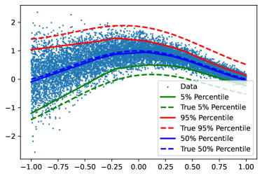
(a) Implicit Quantile Network	(b) Explicit Quantile Network

Figure 1: We trained both implicit and explicit networks on the synthetic data set. The explicit network was trained for three fixed quantile (0.05,0.5,0.95). We see no empirical difference between the two

We train two quantile network, one implicit and one explicit. The explicit network is trained for three fixed quantile (0.05,0.5,0.95). Figure 1 shows fits by both of the networks, we see no empirical difference between the two.

4.2 Traffic Data

We further illustrate our methodology, using data from a sensor on interstate highway I-55. The sensor is located eight miles from the Chicago downtown on I-55 north bound (near Cicero Ave), which is part of a route used by many morning commuters to travel from southwest suburbs to the city. As shown on Figure 2, the sensor is located 840 meters downstream of an off-ramp and 970 meters upstream from an on-ramp.

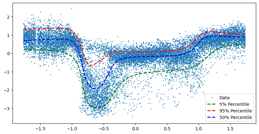
Figure 2: Implicit neural network for traffic speed observed on I-55 north-bound towards Chicago

We can see, a typical day traffic flow pattern on Chicago’s I-55 highway, where sudden breakdowns are followed by a recovery to free flow regime. We can see a breakdown in traffic flow speed during the morning peak period followed by speed recovery. The free flow regimes are usually of little interest to traffic managers. We also, see that variance is low during the free flow regime and high during the breakdown and recovery regimes.

4.3 Satellite Drag

Accurate estimation of satellite drag coefficients in low Earth orbit (LEO) is vital for various purposes such as precise positioning (e.g., to plan maneuvering and determine visibility) and collision avoidance.

Recently, 38 out of 49 Starlink satellites launched by SpaceX on Feb 3, 2022, experienced an early atmospheric re-entry caused by unexpectedly elevated atmospheric drag, an estimated $100MM loss in assets. The launch of the SpaceX Starlink satellites coincided with a geomagnetic storm, which heightened the density of Earth’s ionosphere. This, in turn, led to an elevated drag coefficient for the satellites, ultimately causing the majority of the cluster to re-enter the atmosphere and burn up. This recent accident shows the importance of accurate estimation of drag coefficients in commercial and scientific applications (Berger et al.,, 2023).

Accurate determination of drag coefficients is crucial for assessing and maintaining orbital dynamics by accounting for the drag force. Atmospheric drag is the primary source of uncertainty for objects in LEO. This uncertainty arises partially due to inadequate modeling of the interaction between the satellite and the atmosphere. Drag is influenced by various factors, including geometry, orientation, ambient and surface temperatures, and atmospheric chemical composition, all of which are dependent on the satellite’s position (latitude, longitude, and altitude).

Los Alamos National Laboratory developed the Test Particle Monte Carlo simulator to predict the movement of satellites in low earth orbit (Mehta et al.,, 2014). The simulator takes two inputs, the geometry of the satellite, given by the mesh approximation and seven parameters, which we list in Table 1 below. The simulator takes about a minute to run one scenario and we use a dataset of one million scenarios for the Hubble space telescope (Gramacy,, 2020). The simulator outputs estimates of the drag coefficient based on these inputs, while considering uncertainties associated with atmospheric and gas-surface interaction models (GSI).

Parameter	Range
velocity [m/s]	[5500, 9500]
surface temperature [K]	[100, 500]
atmospheric temperature [K]	[200, 2000]
yaw [radians]	$[-\pi,\pi]$
pitch [radians]	$[-\pi/2,\pi/2]$
normal energy AC [unitless]	[0,1]
tangential momentum AC [unitless]	[0,1]

Table 1: Input parameters for the satellite drag simulator.

We use the data set of 1 million simulation runs provided by sun. The data set has 1 million observations and we use 20% for training and 80% for testing out-of-sample performance. The model architecture is given below. We use the Adam optimizer and a batch size of 2048, and train the model for 200 epochs.

Sauer et al., (2023) provides a survey of modern Gaussian Process based models for prediction and uncertainty quantification tasks. They compare five different models, and apply them to the same Hubble data set we use in this section. We use two metrics to asses the quality of the model, namely RMSE, which captures predictive accuracy, and continuous rank probability score (CRPS; Gneiting and Raftery, (2007); Zamo and Naveau, (2018)). Essentially CRPS is the absolute difference between the predicted and observed cumulative distribution function (CDF). We use the degenerative distribution with the entire mass on the observed value (dirac Delta) as to get the observed CDF. The lower CRPSis better.

Their best performing model is treed-GP has the RMSE of 0.08 and CRPS of 0.04, the worst performing model is the deep GP with approximate “doubly stochastic” variational inference has RMSE of 0.23 and CRPS of 0.16. The best performing model in our experiments is the quantile neural network with RMSE of 0.098 and CRPS of 0.05, which is comparable to the top performer from the survey.

Figure 3 plots of the out-of-sample predictions for forty randomly selected responses (green crosses) and compares those to 50th quantile predictions (orange line) and 95% credible prediction intervals (grey region).

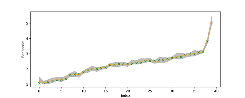
Figure 3: Randomly selected 40 out-of-sample observations from the satellite drag dataset. Green crosses are observed values, orange line is predicted 50% quantile and the grey region is the 95% credible prediction interval.

Figure 4(a) compares the out-of-sample predictions (50% quantiles) $\hat{y}$ and observed drag coefficients $y$. We can see that histogram resambles a normal distribution centered at zero, with some “heaviness” on the left tail, meaning that for some observations, our model under-estimates. The scatterplot in Figure 4(b) shows that the model is more accurate for smaller values of $y$ and less accurate for larger values of $y$ and values of $y$ at around three.

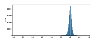
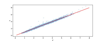
(a) Histogram of errors $\hat{y}-y$	(b) $y$ vs $\hat{y}$

Figure 4: Comparison of out-of-sample predictions (50% quantiles) $\hat{y}$ and observed drag coefficients $y$.

Finally, we show histograms of the posterior predictive distribution for four randomly chosen out-of-sample response values in Figure 5. We can see that the model concentrates the distribution of around the true values of the response.

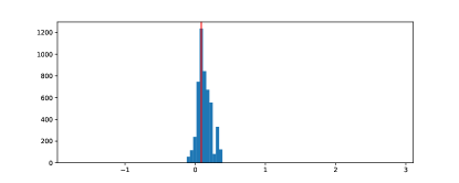
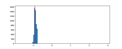
(a) Observation 948127	(b) Observation 722309
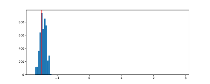
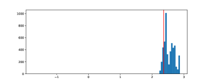
(a) Observation 608936	(b) Observation 988391

Figure 5: Posterior histograms for four randomly chosen out-of-sample response values. The vertical red line is the observed value of the response.

Overall, our model provides a competitive performance to the state-of-the art techniques used for predicting and UQ analysis of complex models, such as satellite drag. The model is able to capture the distribution of the response and provide accurate predictions. The model is also able to provide uncertainty quantification in the form of credible prediction intervals.

5 Discussion

Generative AI is a simulation-based methodology, that takes joint samples of observables and parameters as an input and then applies nonparametric regression in a form of deep neural network by regressing $\theta$ on a non-linear function $h$ which is a function of dimensionality-reduced sufficient statistics of $\theta$ and a randomly generated stochastically uniform error. In its simplest form, $h$, can be identified with its inverse CDF.

One solution to the multi-variate case is to use auto-regressive quantile neural networks. There are also many alternatives to the architecture design that we propose here. For example, autoencoders Albert et al., (2022); Akesson et al., (2021) or implicit models, see Diggle and Gratton, (1984); Baker et al., (2022); Schultz et al., (2022) There is also a link with indirect inference methods developed in Pastorello et al., (2003); Stroud et al., (2003); Drovandi et al., (2011, 2015)

There are many challenging future problems. The method can easily handle high-dimensional latent variables. But designing the architecture for fixed high-dimensional parameters can be challenging. We leave it for the future research. Having learned the nonlinear map, when faced with the observed data $y_{\mathrm{obs}}$, one simply evaluates the nonlinear map at newly generated uniform random values. Generative AI circumvents the need for methods like MCMC that require the density evaluations.

References

- Akesson et al., (2021) Akesson, M., Singh, P., Wrede, F., and Hellander, A. (2021). Convolutional neural networks as summary statistics for approximate bayesian computation. IEEE/ACM Transactions on Computational Biology and Bioinformatics.
- Albert et al., (2022) Albert, C., Ulzega, S., Ozdemir, F., Perez-Cruz, F., and Mira, A. (2022). Learning Summary Statistics for Bayesian Inference with Autoencoders.
- Alvarez and Lawrence, (2011) Alvarez, M. A. and Lawrence, N. D. (2011). Computationally efficient convolved multiple output Gaussian processes. Journal of Machine Learning Research, 12(May):1459–1500.
- Álvarez et al., (2019) Álvarez, M. A., Ward, W., and Guarnizo, C. (2019). Non-linear process convolutions for multi-output gaussian processes. In The 22nd International Conference on Artificial Intelligence and Statistics, pages 1969–1977. PMLR.
- Auld et al., (2016) Auld, J., Hope, M., Ley, H., Sokolov, V., Xu, B., and Zhang, K. (2016). Polaris: Agent-based modeling framework development and implementation for integrated travel demand and network and operations simulations. Transportation Research Part C: Emerging Technologies, 64:101–116.
- Auld et al., (2012) Auld, J., Sokolov, V., Fontes, A., and Bautista, R. (2012). Internet-based stated response survey for no-notice emergency evacuations. Transportation Letters, 4(1):41–53.
- Baker et al., (2022) Baker, E., Barbillon, P., Fadikar, A., Gramacy, R. B., Herbei, R., Higdon, D., Huang, J., Johnson, L. R., Ma, P., Mondal, A., et al. (2022). Analyzing stochastic computer models: A review with opportunities. Statistical Science, 37(1):64–89.
- Banks and Hooten, (2021) Banks, D. L. and Hooten, M. B. (2021). Statistical challenges in agent-based modeling. The American Statistician, 75(3):235–242.
- Barry and Jay M. Ver Hoef, (1996) Barry, R. P. and Jay M. Ver Hoef (1996). Blackbox Kriging: Spatial Prediction without Specifying Variogram Models. Journal of Agricultural, Biological, and Environmental Statistics, 1(3):297–322.
- Bayarri et al., (2007) Bayarri, M. J., Berger, J. O., Paulo, R., Sacks, J., Cafeo, J. A., Cavendish, J., Lin, C.-H., and Tu, J. (2007). A Framework for Validation of Computer Models. Technometrics, 49(2):138–154.
- Beaumont et al., (2002) Beaumont, M. A., Zhang, W., and Balding, D. J. (2002). Approximate Bayesian computation in population genetics. Genetics, 162(4):2025–2035.
- Berger et al., (2023) Berger, T. E., Dominique, M., Lucas, G., Pilinski, M., Ray, V., Sewell, R., Sutton, E. K., Thayer, J. P., and Thiemann, E. (2023). The thermosphere is a drag: The 2022 starlink incident and the threat of geomagnetic storms to low earth orbit space operations. Space Weather, 21(3):e2022SW003330.
- Bernton et al., (2019) Bernton, E., Jacob, P. E., Gerber, M., and Robert, C. P. (2019). Approximate Bayesian computation with the Wasserstein distance. Journal of the Royal Statistical Society: Series B, 81(2):235–269.
- Bhadra et al., (2021) Bhadra, A., Datta, J., Polson, N., Sokolov, V., and Xu, J. (2021). Merging two cultures: Deep and statistical learning. arXiv preprint arXiv:2110.11561.
- Binois et al., (2018) Binois, M., Gramacy, R. B., and Ludkovski, M. (2018). Practical heteroskedastic Gaussian process modeling for large simulation experiments. Journal of Computational and Graphical Statistics, 27(4):808–821.
- Bishop, (1994) Bishop, CM. (1994). Mixture density networks. Technical Report.
- Blum et al., (2013) Blum, M. G. B., Nunes, M. A., Prangle, D., and Sisson, S. A. (2013). A Comparative Review of Dimension Reduction Methods in Approximate Bayesian Computation. Statistical Science, 28(2):189–208.
- Bond-Taylor et al., (2022) Bond-Taylor, S., Leach, A., Long, Y., and Willcocks, C. G. (2022). Deep Generative Modelling: A Comparative Review of VAEs, GANs, Normalizing Flows, Energy-Based and Autoregressive Models. IEEE Transactions on Pattern Analysis and Machine Intelligence, 44(11):7327–7347.
- Bonilla et al., (2008) Bonilla, E. V., Chai, K. M. A., and Williams, C. K. I. (2008). Multi-task Gaussian Process Prediction. Advances in neural information processing systems, page 8.
- Breiman, (2001) Breiman, L. (2001). Statistical modeling: The two cultures (with comments and a rejoinder by the author). Statistical science, 16(3):199–231.
- Brillinger, (2012) Brillinger, D. R. (2012). A Generalized Linear Model With “Gaussian” Regressor Variables. In Guttorp, P. and Brillinger, D., editors, Selected Works of David Brillinger, Selected Works in Probability and Statistics, pages 589–606. Springer, New York, NY.
- Cannon, (2018) Cannon, A. J. (2018). Non-crossing nonlinear regression quantiles by monotone composite quantile regression neural network, with application to rainfall extremes. Stochastic Environmental Research and Risk Assessment, 32(11):3207–3225.
- Caruana, (1997) Caruana, R. (1997). Multitask Learning. Machine Learning, 28(1):41–75.
- Chang et al., (2014) Chang, W., Haran, M., Olson, R., and Keller, K. (2014). Fast dimension-reduced climate model calibration and the effect of data aggregation. The Annals of Applied Statistics, 8(2):649–673.
- Chernozhukov et al., (2010) Chernozhukov, V., Fernández-Val, I., and Galichon, A. (2010). Quantile and Probability Curves Without Crossing. Econometrica, 78(3):1093–1125.
- Conti and O’Hagan, (2010) Conti, S. and O’Hagan, A. (2010). Bayesian emulation of complex multi-output and dynamic computer models. Journal of statistical planning and inference, 140(3):640–651.
- Cortes et al., (2004) Cortes, C., Haffner, P., and Mohri, M. (2004). Rational kernels: Theory and algorithms. Journal of Machine Learning Research, 5(Aug):1035–1062.
- Dabney et al., (2018) Dabney, W., Ostrovski, G., Silver, D., and Munos, R. (2018). Implicit Quantile Networks for Distributional Reinforcement Learning.
- Dabney et al., (2017) Dabney, W., Rowland, M., Bellemare, M. G., and Munos, R. (2017). Distributional Reinforcement Learning with Quantile Regression.
- Diggle and Gratton, (1984) Diggle, P. J. and Gratton, R. J. (1984). Monte Carlo Methods of Inference for Implicit Statistical Models. Journal of the Royal Statistical Society. Series B (Methodological), 46(2):193–227.
- Dixon et al., (2019) Dixon, M. F., Polson, N. G., and Sokolov, V. O. (2019). Deep learning for spatio-temporal modeling: dynamic traffic flows and high frequency trading. Applied Stochastic Models in Business and Industry, 35(3):788–807.
- Donoho, (2000) Donoho, D. L. (2000). High-dimensional data analysis: The curses and blessings of dimensionality. In Ams Conference on Math Challenges of the 21st Century.
- Drovandi et al., (2011) Drovandi, C. C., Pettitt, A. N., and Faddy, M. J. (2011). Approximate Bayesian computation using indirect inference. Journal of the Royal Statistical Society: Series C (Applied Statistics), 60(3):317–337.
- Drovandi et al., (2015) Drovandi, C. C., Pettitt, A. N., and Lee, A. (2015). Bayesian Indirect Inference Using a Parametric Auxiliary Model. Statistical Science, 30(1):72–95.
- Fearnhead and Prangle, (2012) Fearnhead, P. and Prangle, D. (2012). Constructing summary statistics for approximate Bayesian computation: Semi-automatic approximate Bayesian computation. Journal of the Royal Statistical Society: Series B (Statistical Methodology), 74(3):419–474.
- Gattiker et al., (2006) Gattiker, J., Higdon, D., Keller-McNulty, S., McKay, M., Moore, L., and Williams, B. (2006). Combining experimental data and computer simulations, with an application to flyer plate experiments. Bayesian Analysis, 1(4):765–792.
- (37) Gelfand, A. E., Schmidt, A. M., Banerjee, S., and Sirmans, C. (2004a). Nonstationary multivariate process modeling through spatially varying coregionalization. Test, 13(2):263–312.
- (38) Gelfand, A. E., Schmidt, A. M., Banerjee, S., and Sirmans, C. F. (2004b). Nonstationary multivariate process modeling through spatially varying coregionalization. Test, 13(2):263–312.
- Genton and Kleiber, (2015) Genton, M. G. and Kleiber, W. (2015). Cross-covariance functions for multivariate geostatistics. Statistical Science, 30(2):147–163.
- Germain et al., (2015) Germain, M., Gregor, K., Murray, I., and Larochelle, H. (2015). MADE: Masked Autoencoder for Distribution Estimation. In Proceedings of the 32nd International Conference on Machine Learning, pages 881–889. PMLR.
- Gneiting and Raftery, (2007) Gneiting, T. and Raftery, A. E. (2007). Strictly proper scoring rules, prediction, and estimation. Journal of the American statistical Association, 102(477):359–378.
- Goodfellow et al., (2020) Goodfellow, I., Pouget-Abadie, J., Mirza, M., Xu, B., Warde-Farley, D., Ozair, S., Courville, A., and Bengio, Y. (2020). Generative adversarial networks. Communications of the ACM, 63(11):139–144.
- Goulard and Voltz, (1992) Goulard, M. and Voltz, M. (1992). Linear coregionalization model: tools for estimation and choice of cross-variogram matrix. Mathematical Geology, 24(3):269–286.
- Gramacy, (2020) Gramacy, R. B. (2020). Surrogates: Gaussian process modeling, design, and optimization for the applied sciences. CRC press.
- Gramacy and Apley, (2015) Gramacy, R. B. and Apley, D. W. (2015). Local Gaussian Process Approximation for Large Computer Experiments. Journal of Computational and Graphical Statistics, 24(2):561–578.
- Gramacy and Lee, (2008) Gramacy, R. B. and Lee, H. K. H. (2008). Bayesian Treed Gaussian Process Models With an Application to Computer Modeling. Journal of the American Statistical Association, 103(483):1119–1130.
- Heaton et al., (2017) Heaton, J. B., Polson, N. G., and Witte, J. H. (2017). Deep learning for finance: deep portfolios. Applied Stochastic Models in Business and Industry, 33(1):3–12.
- Higdon, (2002) Higdon, D. (2002). Space and space-time modeling using process convolutions. In Quantitative methods for current environmental issues, pages 37–56. Springer.
- Izmailov et al., (2021) Izmailov, P., Vikram, S., Hoffman, M. D., and Wilson, A. G. G. (2021). What are bayesian neural network posteriors really like? In International conference on machine learning, pages 4629–4640. PMLR.
- Jiang et al., (2017) Jiang, B., Wu, T.-Y., Zheng, C., and Wong, W. H. (2017). Learning Summary Statistic For Approximate Bayesian Computation Via Deep Neural Network. Statistica Sinica, 27(4):1595–1618.
- Jiang et al., (2018) Jiang, B., Wu, Tung-Yu, and Wing Hung Wong (2018). Approximate Bayesian Computation with Kullback-Leibler Divergence as Data Discrepancy. In Proceedings of the Twenty-First International Conference on Artificial Intelligence and Statistics, pages 1711–1721. PMLR.
- Kingma and Welling, (2022) Kingma, D. P. and Welling, M. (2022). Auto-Encoding Variational Bayes.
- Kolmogorov, (1942) Kolmogorov, AN. (1942). Definition of center of dispersion and measure of accuracy from a finite number of observations (in Russian). Izv. Akad. Nauk SSSR Ser. Mat., 6:3–32.
- Lázaro-Gredilla et al., (2010) Lázaro-Gredilla, M., Quinonero-Candela, J., Rasmussen, C. E., and Figueiras-Vidal, A. R. (2010). Sparse spectrum gaussian process regression. The Journal of Machine Learning Research, 11:1865–1881.
- Longstaff and Schwartz, (2001) Longstaff, F. A. and Schwartz, E. S. (2001). Valuing American options by simulation: A simple least-squares approach. The review of financial studies, 14(1):113–147.
- Mardia and Goodall, (1993) Mardia, K. V. and Goodall, C. R. (1993). Spatial-temporal analysis of multivariate environmental monitoring data. Multivariate environmental statistics, 6(76):347–385.
- Mehta et al., (2014) Mehta, P. M., Walker, A., Lawrence, E., Linares, R., Higdon, D., and Koller, J. (2014). Modeling satellite drag coefficients with response surfaces. Advances in Space Research, 54(8):1590–1607.
- Myers, (1984) Myers, D. E. (1984). Co-Kriging — New Developments. In Verly, G., David, M., Journel, A. G., and Marechal, A., editors, Geostatistics for Natural Resources Characterization: Part 1, pages 295–305. Springer Netherlands.
- Müller et al., (1997) Müller, P., West, M., and MacEachern, S. N. (1997). Bayesian models for non-linear auto-regressions. Journal of Time Series Analysis, 18:593–614.
- Nareklishvili et al., (2022) Nareklishvili, M., Polson, N., and Sokolov, V. (2022). Deep partial least squares for IV regression. arXiv preprint arXiv:2207.02612.
- Nunes and Balding, (2010) Nunes, M. A. and Balding, D. J. (2010). On Optimal Selection of Summary Statistics for Approximate Bayesian Computation. Statistical Applications in Genetics and Molecular Biology, 9(1).
- Osborne et al., (2009) Osborne, M. A., Garnett, R., and Roberts, S. J. (2009). Gaussian processes for global optimization. In 3rd international conference on learning and intelligent optimization (LION3), pages 1–15.
- Ostrovski et al., (2018) Ostrovski, G., Dabney, W., and Munos, R. (2018). Autoregressive Quantile Networks for Generative Modeling.
- Papamakarios and Murray, (2016) Papamakarios, G. and Murray, I. (2016). Fast \epsilon -free Inference of Simulation Models with Bayesian Conditional Density Estimation. In Advances in Neural Information Processing Systems, volume 29. Curran Associates, Inc.
- Papamakarios et al., (2017) Papamakarios, G., Pavlakou, T., and Murray, I. (2017). Masked Autoregressive Flow for Density Estimation. In Advances in Neural Information Processing Systems, volume 30. Curran Associates, Inc.
- Park et al., (2016) Park, M., Jitkrittum, W., and Sejdinovic, D. (2016). K2-ABC: Approximate Bayesian Computation with Kernel Embeddings. In Proceedings of the 19th International Conference on Artificial Intelligence and Statistics, pages 398–407. PMLR.
- Parzen, (2004) Parzen, E. (2004). Quantile Probability and Statistical Data Modeling. Statistical Science, 19(4):652–662.
- Pastorello et al., (2003) Pastorello, S., Patilea, V., and Renault, E. (2003). Iterative and recursive estimation in structural nonadaptive models. Journal of Business & Economic Statistics, 21(4):449–509.
- Polson and Sokolov, (2017) Polson, N. and Sokolov, V. (2017). Deep learning for short-term traffic flow prediction. Transportation Research Part C: Emerging Technologies, 79:1–17.
- Polson et al., (2021) Polson, N., Sokolov, V., and Xu, J. (2021). Deep learning partial least squares. arXiv preprint arXiv:2106.14085.
- Polson and Ročková, (2018) Polson, N. G. and Ročková, V. (2018). Posterior concentration for sparse deep learning. Advances in Neural Information Processing Systems, 31.
- Reich et al., (2011) Reich, B. J., Eidsvik, J., Guindani, M., Nail, A. J., and Schmidt, A. M. (2011). A class of covariate-dependent spatiotemporal covariance functions for the analysis of daily ozone concentration. Annals of Applied Statistics, 5(4):2425–2447.
- Rezende and Mohamed, (2015) Rezende, D. J. and Mohamed, S. (2015). Variational inference with normalizing flows. arXiv preprint arXiv:1505.05770.
- Sauer et al., (2023) Sauer, A., Cooper, A., and Gramacy, R. B. (2023). Non-stationary gaussian process surrogates. arXiv preprint arXiv:2305.19242.
- Schmidt et al., (2011) Schmidt, A. M., Guttorp, P., and O’Hagan, A. (2011). Considering covariates in the covariance structure of spatial processes. Environmetrics, 22(4):487–500.
- Schultz et al., (2022) Schultz, L., Auld, J., and Sokolov, V. (2022). Bayesian Calibration for Activity Based Models. arXiv preprint arXiv:2203.04414.
- Shan and Wang, (2010) Shan, S. and Wang, G. G. (2010). Survey of modeling and optimization strategies to solve high-dimensional design problems with computationally-expensive black-box functions. Structural and Multidisciplinary Optimization, 41(2):219–241.
- Sohl-Dickstein et al., (2015) Sohl-Dickstein, J., Weiss, E. A., Maheswaranathan, N., and Ganguli, S. (2015). Deep Unsupervised Learning using Nonequilibrium Thermodynamics.
- Sokolov, (2017) Sokolov, V. (2017). Discussion of ‘deep learning for finance: deep portfolios’. Applied Stochastic Models in Business and Industry, 33(1):16–18.
- Stroud et al., (2003) Stroud, J. R., Müller, P., and Polson, N. G. (2003). Nonlinear state-space models with state-dependent variances. Journal of the American Statistical Association, 98(462):377–386.
- Teh et al., (2005) Teh, Y. W., Seeger, M., and Jordan, M. I. (2005). Semiparametric latent factor models. In International Workshop on Artificial Intelligence and Statistics, pages 333–340.
- van den Oord and Kalchbrenner, (2016) van den Oord, A. and Kalchbrenner, N. (2016). Pixel RNN. In ICML.
- Wang et al., (2022) Wang, Y., Polson, N., and Sokolov, V. O. (2022). Data augmentation for bayesian deep learning. Bayesian Analysis, 1(1):1–29.
- Wang and Ročková, (2022) Wang, Y. and Ročková, V. (2022). Adversarial bayesian simulation. arXiv preprint arXiv:2208.12113.
- Wilson et al., (2014) Wilson, A. G., Gilboa, E., Nehorai, A., and Cunningham, J. P. (2014). Fast kernel learning for multidimensional pattern extrapolation. Advances in neural information processing systems, 27.
- Yaari, (1987) Yaari, M. E. (1987). The Dual Theory of Choice under Risk. Econometrica, 55(1):95–115.
- Zamo and Naveau, (2018) Zamo, M. and Naveau, P. (2018). Estimation of the continuous ranked probability score with limited information and applications to ensemble weather forecasts. Mathematical Geosciences, 50(2):209–234.