Quasi-Deterministic Burstiness Bound for Aggregate of Independent, Periodic Flows

Abstract

Time-sensitive networks require timely and accurate monitoring of the status of the network. To achieve this, many devices send packets periodically, which are then aggregated and forwarded to the controller. Bounding the aggregate burstiness of the traffic is then crucial for effective resource management. In this paper, we are interested in bounding this aggregate burstiness for independent and periodic flows. A deterministic bound is tight only when flows are perfectly synchronized, which is highly unlikely in practice and would be overly pessimistic. We compute the probability that the aggregate burstiness exceeds some value. When all flows have the same period and packet size, we obtain a closed-form bound using the Dvoretzky–Kiefer–Wolfowitz inequality. In the heterogeneous case, we group flows and combine the bounds obtained for each group using the convolution bound. Our bounds are numerically close to simulations and thus fairly tight. The resulting aggregate burstiness estimated for a non-zero violation probability is considerably smaller than the deterministic one: it grows in $\sqrt{n\log{n}}$, instead of $n$, where $n$ is the number of flows.

1 Introduction

The development of industrial automation requires timely and accurate monitoring of the status of the network. In time-sensitive networks, a common assumption for critical types of traffic is that devices send packets periodically. These packets are aggregated and forwarded to the controller. Characterizing this aggregate traffic is then crucial for effective resource management.

Among the analytic tools providing analysis for real-time systems is deterministic network calculus [13, 1]. From the characterization of the flows, the description of the switches (offered bandwidth and scheduling policy), it can derive worst-case performance bounds, such as end-to-end delay or buffer occupancy. These performances can grow linearly with the burstiness of the flows [3]. Hence, accurately bounding the burstiness is key for performance evaluation and resource management. However, deterministic network calculus takes into account the worst-case scenario for aggregation of flows, which happens when flows are perfectly synchronized, and this is very unlikely to happen.

To overcome this issue, probabilistic versions of network calculus (known as Stochastic Network Calculus) have emerged, and their aim is to compute performances when a small violation probability is allowed. Using probabilistic tools such as moment-generating functions [8] or martingales [15], recent works mainly focus on ergodic systems and on the performances at an arbitrary point in time. This does not imply that the probability that the delay bound is never violated during a period of interest is small. Moreover, results are very limited in terms of topology and service policies, and become inaccurate for multiple servers [2]. Methods that compute probabilistic bounds on the burstiness have been discarded as they do not provide as good results for ergodic systems [6].

In this paper, we focus on the burstiness of the aggregation of periodic and independent flows. In other words, each flow sends packets periodically with a fixed packet size and period. The first packet is sent at a random time (the phase) within that period. We assume phases are mutually independent. Our aim is to find a probabilistic bound on the burstiness of the aggregation of flows, that is, finding a burst that is valid at all times with large probability. That way, combining these probabilistic burstiness bounds with results of deterministic network calculus lead to delay and backlog bounds that are valid with large probability at all times, hence the name quasi-deterministic. To our knowledge, this is the first method to obtain quasi-deterministic bounds for independent, periodic flows.

Our contributions are the following:

1. First, in the homogeneous setting, where all flows have the same period and packet size, we provide two probabilistic bounds for the aggregate burstiness. Both of them are based on bounding the probability of some event $E$ relying on the order statistics of the phases. The former (Theorem 4.1) has a closed form; it uses the Dvoretzky–Kiefer–Wolfowitz (DKW) inequality [14] to bound the probability of $E$, and when a small positive violation probability is allowed, the burstiness grows in $O(\sqrt{n\log{n}})$, where $n$ is the number of flows, instead of $O(n)$ for a deterministic bound. The latter (Theorem 4.2) directly computes the probability of $E$, which can be implemented iteratively.

2. Second, we focus on two types of heterogeneity: either flows can be grouped into several homogeneous sub-sets, and we use a bounding technique based on convolution (Theorem 5.1), or flows have the same period but different packet sizes, and the bounds can be adapted from the homogeneous case (Theorem 5.2).

3. Last, we numerically show that our bounds are close to simulations. The quasi-deterministic aggregate burstiness we obtain with a small, non-zero violation tolerance is considerably smaller than the deterministic one. For the heterogeneous case, we show that our convolution bounding technique provides bounds significantly smaller than those obtained by the union bound.

The rest of the paper is organized as follows: We present our model in Section 2, and then in Section 3 some results from state of the art. Our contributions are detailed in Section 4 for the homogeneous case and Section 5 for the heterogeneous case. Finally, we provide some simulation results in Section 6 to demonstrate the tightness of the bounds.

2 Assumptions and Problem Statement

We use the notation $\mathbb{N}=\{0,1,\ldots\}$ and $\mathbb{N}_{n}=\{1,\ldots,n\}$.

Assumptions

We consider $n$ periodic flows of packets. Each flow $f\in\mathbb{N}_{n}$ is periodic with period $\tau_{f}$ and phase $\phi_{f}\in[0,\tau_{f})$, and sends packets of size $\ell_{f}$: the number of bits of flow $f$ arriving in the time interval $[0,t)$ is $\ell_{f}\lceil[t-\phi_{f}]^{+}/\tau_{f}\rceil$ where we use the notation $[x]^{+}=\max(0,x)$ and $\lceil\rceil$ denotes the ceiling.

For every flow $f$, we assume that $\phi_{f}$ is random, uniformly distributed in $[0,\tau_{f}]$, and that the different $(\phi_{f})_{f\in\mathbb{N}_{n}}$ are independent random variables.

Problem Statement

We consider the aggregation of the $n$ flows and let $A[s,t)$ denote the number of bits observed in time interval $[s,t)$. Our goal is to find a token-bucket arrival curve constraining this aggregate, that is, a rate $r$ and a burst $b$ such that $\forall s\leq t,~{}A[s,t)\leq r(t-s)+b$. It follows from the assumptions that each individual flow $f\in\mathbb{N}_{n}$ is constrained by a token-bucket arrival curve with rate $r_{f}=\ell_{f}/\tau_{f}$ and burst $\ell_{f}$. Therefore, the aggregate flow is constrained by a token-bucket arrival curve with rate $r^{\scriptsize\textrm{tot}}=\sum_{f=1}^{n}r_{f}$ and burst $\ell^{\scriptsize\textrm{tot}}=\sum_{f=1}^{n}\ell_{f}$.

However, due to the randomness of the phases, $\ell^{\scriptsize\textrm{tot}}$ might be larger than what is observed, and we are rather interested in token-bucket arrival curves with rate $r^{\scriptsize\textrm{tot}}$ and a burst $b$ valid with some probability; specifically, we want to find a bound on the tail probability of the aggregate burstiness, which is defined as the smallest value of $B$ such that the aggregate flow is constrained by a token-bucket arrival curve with rate $r^{\scriptsize\textrm{tot}}$ and burst $B$, for the entire network lifetime. The aggregate burstiness is given by

$$B=\sup_{t\geq 0}\bar{B}(t).$$ (1)

where $\bar{B}(t)$ is the token-bucket content at time $t$ for a token-bucket that is initially empty, and is given by

$$\bar{B}(t)=\sup_{s\leq t}\{A[s,t)-r^{\scriptsize\textrm{tot}}(t-s)\}.$$ (2)

Note that $B$ is a function of the random phases of the flows, therefore, is also random. Assume that $\mathds{P}(B>b)=\varepsilon$; this means that, with probability $1-\varepsilon$, after periodic flows started, the aggregate burstiness is $\leq b$. Conversely, with probability $\varepsilon$, the aggregate burstiness is $>b$.

Observe that $\mathds{P}(B>b)=0$ for all $b\geq\ell^{\scriptsize\textrm{tot}}$, as $\ell^{\scriptsize\textrm{tot}}$ is a deterministic bound on the aggregate burstiness. Then, for some pre-specified value $0\leq b<\ell^{\scriptsize\textrm{tot}}$, our problem is equivalent to finding $\epsilon(b)$ that bounds the tail probability of the aggregate burstiness $B$, i.e.,

$$\mathds{P}(B>b)\leq\epsilon(b).$$ (3)

3 Background and Related Works

Bounding the burstiness of flows in Network Calculus is an important problem since it has a strong influence on the delay and backlog bounds. The deterministic aggregate burstiness can be improved (compared with summing burstiness of all flows) when the phases of the flows are known exactly [7].

Regarding the stochastically bounded burstiness [6, 11], three models have been proposed, depending on how quantifiers are used,

$$\textrm{SBB}:\forall 0\leq s\leq t,~{}\mathds{P}\left(A[s,t)-r(t-s)>b\right)\leq\epsilon(b),$$ (4)

$$\textrm{S}^{2}\textrm{BB}:\forall t\geq 0,~{}\mathds{P}(\sup_{0\leq s\leq t}\{A[s,t)-r(t-s)\}>b)\leq\epsilon(b),$$ (5)

$$\textrm{S}^{3}\textrm{BB}:\mathds{P}(\sup_{t\geq 0}\{\sup_{0\leq s\leq t}\{A[s,t)-r(t-s)\}\}>b)\leq\epsilon(b).$$ (6)

First, notice that $\textrm{S}^{3}\textrm{BB}\implies\textrm{S}^{2}\textrm{BB}\implies\textrm{SBB}$. Indeed, SBB is a probability upper bound that the arrival curve constraint is invalid for a fixed pair of times $s\leq t$. In contrast, $\textrm{S}^{2}\textrm{BB}$ is the probability that token-bucket content at time $t$, $\bar{B}(t)$ exceeds $b$, hence the “$\forall s$” appearing inside the probability. Last, $\textrm{S}^{3}\textrm{BB}$ represents the violation probability of the aggregate burstiness $B$ of the whole process. A deterministic arrival curve is a special case of $\textrm{S}^{3}\textrm{BB}$, with $\epsilon(b)=0$, which is why, for a non-zero violation probability $\epsilon(b)$, $b$ is called a quasi-deterministic bound on the burstiness.

The first model SBB is the weakest, but also the easiest to handle: bounding the arrivals during a given interval of time can be done for many stochastic models. It was also used for the study of aggregated independent flows with periodic patterns [16, 4, 8, 6, 10, 12]. All the approaches can be summarized as follows: a) defining an event $E_{s}$ of interest related to some time interval $[s,t)$ and aggregation of the flows; b) combining the events $(E_{s})_{s\leq t}$ together to obtain a violation probability of the burstiness or of the backlog bound at time $t$.

The second model $\textrm{S}^{2}\textrm{BB}$ seems at first more adapted to network calculus analysis, as performance bounds can be directly derived from the formulation. However, the probability bound of $\textrm{S}^{2}\textrm{BB}$ is usually deduced from SBB, which leads to pessimistic bounds for a single server. Nevertheless, this framework may become necessary for more complex cases [5].

In time-sensitive networks, we are interested in the probability that a delay or backlog bound is not violated during some interval (e.g., the network’s lifetime), not just one arbitrary point in time, so the two models SBB and $\textrm{S}^{2}\textrm{BB}$ are not adapted, as they do not provide the violation probability of a delay bound during a whole period of interest. In contrast, when using $\textrm{S}^{3}\textrm{BB}$, we can guarantee, with some probability, that delay and backlog bounds derived by deterministic network calculus are never violated during the network’s lifetime, which is why we choose this formulation in our model.

As pointed out in [6, Section 4.4], when arrival processes are stationary and ergodic, $\textrm{S}^{3}\textrm{BB}$ is always trivial and the bounding function $\epsilon(b)$ in (6) is either zero or one. This is perhaps why the literature was discouraged from studying $\textrm{S}^{3}\textrm{BB}$ characterizations. However, it has been overlooked that there is interest in some non-ergodic arrival processes, as in our case. Indeed, with our model, phases $\phi_{f}$ are drawn randomly but remain the same during the entire period of interest; thus, our arrival processes are not ergodic.

4 Homogeneous Case

In this section, we consider the case where flows have the same packet size and same period.

More precisely, we assume

• There exist $\tau,\ell>0$ such that $\forall f\in\mathbb{N}_{n},~{}\ell_{f}=\ell,\tau_{f}=\tau$ and $(\phi_{f})_{f\in\mathbb{N}_{n}}$ is a family of independent and identically distributed (iid) uniform random variables (rv) on $[0,\tau)$.

We present two bounds for the aggregate burstiness; the former gives a closed form, unlike the latter, which might be slightly more accurate when the number of flows is small.

Let us first prove a useful result when the period $\tau$ is equal to $1$; it shows that if the time origin is shifted to the arrival time of the first packet of flow $i$, the phases of the $n-1$ other flows remain uniformly distributed on $[0,1)$ and mutually independent. For this, we define the function $h$ as $\forall x,y\in[0,1)$,

$$h(x,y)=(x-y)\mathds{1}_{x\geq y}+(1+x-y)\mathds{1}_{x<y}.$$ (7)

Intuitively, if $x=\phi_{j}$ and $y=\phi_{i}$, $h(x,y)$ is the time until the arrival of the first packet of flow $j$, counted from the arrival time of the first packet of flow $i$.

Lemma 1

Let $U_{1},\ldots,U_{n}$ be a sequence of $n$ iid uniform rv on $[0,1)$. Let $i\in\mathbb{N}_{n}$ and define $W_{j}$ for $j\in\mathbb{N}_{n}\setminus\{i\}$ by $W_{j}=h(U_{j},U_{i})$. Then, $(W_{j})_{j\neq i}$ is a family of $n-1$ iid uniform rv on $[0,1)$.

Proof

Let us first do a preliminary computation for all $u_{i}\in[0,1]$ and all bounded measurable function $g_{j}$:

$$\mathds{E}[g_{j}(h(U_{j},u_{i}))]=\int_{u_{j}=0}^{1}g_{j}(h(u_{j},u_{i}))du_{j} =\int_{u_{j}=u_{i}}^{1}g_{j}(u_{j}-u_{i})du_{j}+\int_{u_{j}=0}^{u_{i}}g_{j}(1+u_{j}-u_{i})du_{j}$$

$$=\int_{u_{j}=0}^{1-u_{i}}g_{j}(w_{j})dw_{j} +\int_{u_{j}=1-u_{i}}^{1}g_{j}(w_{j})dw_{j}=\int_{w_{j}=0}^{1}g_{j}(w_{j})dw_{j}.$$

Then, consider a collection of bounded measurable functions $(g_{j})_{j\neq i}$: we can compute $\mathds{E}[\prod_{j\neq i}g_{j}(W_{j})]=\mathds{E}[\prod_{j\neq i}g_{j}(h(U_{j},U_{i}))]=\int_{u_{i}=0}^{1}\mathds{E}[\prod_{j\neq i}g_{j}(h(U_{j},u_{i}))]du_{i}=\int_{0}^{1}\prod_{j\neq i}\mathds{E}[g_{j}(h(U_{j},u_{i}))]du_{i}=\int_{0}^{1}\prod_{j\neq i}\mathds{E}[g_{j}(V_{j})]du_{i}=\prod_{j\neq i}\mathds{E}[g_{j}(V_{j})]=\mathds{E}[\prod_{j\neq i}g_{j}(V_{j})]$, where $(V_{j})_{j\neq j}$ is a collection of $n-1$ iid uniformly rv on $[0,1)$. ∎

The bounds we are to present are based on the order statistics: consider $n-1$ rv $U_{1},\ldots,U_{n-1}$ and its order statistics is $U_{(1)}\leq\cdots\leq U_{(n-1)}$, defined by sorting $U_{1},\ldots,U_{n-1}$ in non-decreasing order. It is well-known [9, Equation 1.145] that if $(U_{i})$ is an iid family of uniform rv on [0,1], the density function of the joint distribution of $U_{(1)},\ldots,U_{(n-1)}$ is

$$f_{U_{(1)},\ldots,U_{(n-1)}}(y_{1},\ldots,y_{n-1})=(n-1)!\mathds{1}_{0\leq y_{1}\leq y_{2}\leq\ldots\leq y_{n-1}\leq 1}.$$ (8)

The next proposition connects the order statistics of the phases with the aggregate burstiness, and is key for Theorems 4.1 and 4.2.

Proposition 1

Assume model ${\bf(H).}$ For all $0\leq b<n\ell$,

$$\mathds{P}(B>b)\leq n\mathds{P}(E),$$ (9)

with

$$E\overset{\scriptsize\textit{def}}{=}\bigcup_{k=\lfloor b/\ell\rfloor}^{n-1}\left\{U_{(k)}<\frac{(k+1)-b/\ell}{n}\right\},$$ (10)

where $U_{(1)},\ldots,U_{(n-1)}$ is the order statistic of $n-1$ iid uniform rv on $[0,1]$.

Proof

Note that the normalized process $\tilde{A}[s,t)=\frac{1}{\ell}A[\tau s,\tau t)$ follows model ${\bf(H)}$ with $\tau=\ell=1$, and

$$\mathds{P}(B>b)=\mathds{P}(\tilde{B}>b/\ell).$$

We then assume in this proof (and that of Theorem 4.1) that $\tau=\ell=1$, and the final result is obtained by replacing $b$ by $b/\ell$. One can also remark that the bound is independent of $\tau$.

Let $T_{j},~{}j\geq 1$ be the arrival time of the $j$-th packet in the aggregate. With probability 1, $T_{j}$ is strictly increasing as we assume all phases are different. First, for all $i\leq j$, for all $(t_{i},t_{j})\in(T_{i-1},T_{i}]\times(T_{j},T_{j+1}]\overset{\scriptsize\textit{def}}{=}C_{i,j}$, $A[t_{i},t_{j})=j-i+1$, and $H_{i,j}\overset{\scriptsize\textit{def}}{=}\sup_{t_{i},t_{j}\in C_{i,j}}A[t_{i},t_{j})-n(t_{i}-t_{j})=j-i+1-n(T_{j}-T_{i})$. Then, we can rewrite the aggregate burstiness as

$$B=\sup_{1\leq i\leq j}\sup_{t_{i},t_{j}\in C_{i,j}}A[t_{i},t_{j})-n(t_{i}-t_{j})=\sup_{1\leq i\leq j}H_{i,j}.$$ (11)

As our model is the aggregation of $n$ flows of period 1, $T_{j+n}=T_{j}+1$ for $j\geq 1$, and $H_{i,j+n}=j+n-i+1-n(T_{j}-1-T_{i})=H_{i,j}$ for all $j\geq i$. Similarly, $H_{i+n,j}=H_{i,j}$ for all $j\geq i+n$. Combine this with (11) and obtain

$$B=\max_{j\geq 1}~{}\max_{i\in\mathbb{N}_{j}}H_{i,j}=\max_{i\in\mathbb{N}_{n}}\underbrace{\max_{i\leq j\leq n-1}H_{i,j}}_{B_{i}}.$$ (12)

We now prove that $\forall i\in\mathbb{N}_{n}$, $\mathds{P}\left(B_{i}>b\right)=\mathds{P}(E)$.

Observe that for all $j\geq i$, we have the equality of events $\{H_{i,j}>b\}=\{T_{j}-T_{i}<(j-i+1-b)/n\}$, so for all $i\in\mathbb{N}_{n}$, $\left\{B_{i}>b\right\}=\bigcup_{j=i}^{i+n-1}\left\{T_{j}-T_{i}<(j-i+1-b)/n\right\}$.

We can also notice that the sequence $(T_{j}-T_{i})_{j=i+1}^{n+i-1}$ is the ordered sequence of phases starting from time origin $T_{i}$. Conditionally to $T_{i}=\phi_{f}$, or equivalently $\phi_{(i)}=f$, $(T_{j}-T_{i})_{j=i+1}^{n+i-1}$ is the order statistics of $(\phi_{j}-\phi_{f})_{j\neq f}$, which is, from Lemma 1, iid and uniformly distributed on $[0,1)$. If follows that

$$\mathds{P}(B_{i}>b~{}|~{}\phi_{(i)}=f)=\mathds{P}(\cup_{k=1}^{n-1}\{U_{(k)}<\frac{k-b}{n}\})=\mathds{P}(\cup_{k=\lfloor b\rfloor}^{n-1}\{U_{(k)}<\frac{k-b}{n}\})=\mathds{P}(E),$$

since $U_{(k)}\geq 0$. Then, using the law of total probabilities, $\mathds{P}(B_{i}>b)=\sum_{f=1}^{n}\mathds{P}(B_{i}>b~{}|~{}\phi_{(i)}=f)\mathds{P}(\phi_{(i)}=f)=\mathds{P}(E)$.

Lastly, we conclude by using the union bound: $\mathds{P}(B>b)=\mathds{P}(\cup_{i=1}^{n}B_{i}>b)\leq\sum_{i=1}^{n}\mathds{P}(B_{i}>b)=n\mathds{P}(E)$. ∎

We now present the first bound on the tail probability of the aggregate burstiness $B$.

Theorem 4.1 (Homogeneous case, DKW bound)

Assume model ${\bf(H)}$ with $n>1$. For all $b<n\ell$, a bound on the tail probability of the aggregate burstiness $B$ is given by

$$\mathds{P}\left(B>b\right)\leq n\;\exp{\left(-2(n-1)\left(\frac{\lfloor b/\ell\rfloor}{n-1}-\frac{1}{n}\right)^{2}\right)}\overset{\scriptsize\textit{def}}{=}\varepsilon^{\scriptsize\textrm{dkw}}(n,\ell,b).$$ (13)

Proof

Let us assume that $\tau=\ell=1$ in the proof, as in the proof of Proposition 1. Observe that when $\lfloor b\rfloor<1-\frac{1}{n}+\sqrt{\frac{(n-1)\log 2}{2}}$, we have $\varepsilon^{\scriptsize\textrm{dkw}}(n,1,b)\geq\frac{n}{2}$, hence (13) holds. Therefore we now proceed to prove (13) when $\lfloor b\rfloor\geq 1-\frac{1}{n}+\sqrt{\frac{(n-1)\log 2}{2}}$.

Step 1: Consider $n-1$ iid, rv $U_{1},\ldots,U_{n-1}$ and its order statistics is $U_{(1)}\leq\cdots\leq U_{(n-1)}$, defined by sorting $U_{1},\ldots,U_{n-1}$ in non-decreasing order. For $\varepsilon>0$, define $E^{\prime}(\varepsilon)$ by

$$E^{\prime}(\varepsilon)\overset{\scriptsize\textit{def}}{=}\bigcup_{k=1}^{n-1}\left\{U_{(k)}<\frac{k}{n-1}-\varepsilon\right\}.$$ (14)

We now show that if $\varepsilon\geq\sqrt{\frac{\log 2}{2(n-1)}}$,

$$\mathds{P}\left(E^{\prime}(\varepsilon)\right)\leq e^{-2(n-1)\varepsilon^{2}}.$$ (15)

Let $F_{n-1}$ be the (random) empirical cumulative distribution function of $U_{1},\ldots,U_{n-1}$, defined $\forall x\in[0,1]$ by

$$F_{n-1}(x)=\frac{1}{n-1}\sum_{i=1}^{n-1}\mathds{1}_{U_{(i)}\leq x}.$$ (16)

The Dvoretzky–Kiefer–Wolfowitz inequality [14] states that if $\varepsilon\geq\sqrt{\frac{\log 2}{2(n-1)}}$, then

$$\mathds{P}\big{(}\sup_{x\in[0,~{}1]}(F_{n-1}(x)-x)>\varepsilon\big{)}\leq e^{-2(n-1)\varepsilon^{2}}.$$ (17)

We can apply this to find the bound of interest. First, we prove that

$$\sup_{x\in[0,~{}1]}(F_{n-1}(x)-x)>\varepsilon\Leftrightarrow\exists k\in\mathbb{N}_{n-1},~{}U_{(k)}<\frac{k}{n-1}-\varepsilon.$$ (18)

Proof of $\Leftarrow$: First, observe that $F_{n-1}(U_{(k)})=k/(n-1)$, so if $\frac{k}{n-1}-U_{(k)}>\varepsilon$ for some $k$, then $F_{n-1}\left(U_{(k)}\right)-U_{(k)}>\varepsilon$, and the left-hand side holds.

Proof of $\Rightarrow$: Set $U_{(0)}=0$ and $U_{(n)}=1$. Observe that for all $k\in\{0,\ldots,n-1\}$, and all $U_{(k)}\leq x<U_{(k+1)}$, $F_{n-1}\left(x\right)=F_{n-1}\left(U_{(k)}\right)=\frac{k}{n-1}$. Hence, $F_{n-1}(x)-x=\frac{k}{n-1}-x$ is decreasing on each segment $[U_{(k)},U_{(k+1)})$. Then, the supremum in the left-hand side of (18) is obtained for some $x=U_{(k)}$, i.e., $\sup_{x\in[0,~{}1]}(F_{n-1}(x)-x)=\sup_{k\in\{0,\ldots,n-1\}}(F_{n-1}(U_{(k)})-U_{(k)})=\sup_{k\in\{0,\ldots,n-1\}}(\frac{k}{n-1}-U_{(k)})$, which implies the right-hand side ($F_{n-1}(0)-0=0<\varepsilon$).

This proves (18), and Step 1 is concluded by combining it with (17).

Step 2: We now proceed to show that if

$$\varepsilon=\frac{\lfloor b\rfloor}{n-1}-\frac{1}{n},$$ (19)

then, $E\subseteq E^{\prime}(\varepsilon)$, where event $E$ is defined in Proposition 1.

It is enough to show that for all $k\in\{\lfloor b\rfloor,\ldots,n-1\}$, $\frac{k+1-b}{n}\leq\frac{k-\lfloor b\rfloor}{n-1}+\frac{1}{n}$, which can be deduced from the following implications:

$$\frac{k+1-b}{n}\leq\frac{k-\lfloor b\rfloor}{n-1}+\frac{1}{n}\Leftrightarrow\frac{k-b}{n}\leq\frac{k-\lfloor b\rfloor}{n-1}\Leftarrow\frac{k-\lfloor b\rfloor}{n}\leq\frac{k-\lfloor b\rfloor}{n-1}\Leftrightarrow\frac{1}{n}\leq\frac{1}{n-1}.$$

Step 3: By Step 2, we have $\mathds{P}(E)\leq\mathds{P}(E^{\prime}(\varepsilon))$. Also, observe that $\lfloor\frac{b}{l}\rfloor\geq 1-\frac{1}{n}+\sqrt{\frac{(n-1)\log 2}{2}}$ implies $\varepsilon\geq\sqrt{\frac{\log 2}{2(n-1)}}$. Thus, combine it with Step 1 to obtain

$$\mathds{P}(E)\leq\mathds{P}(E^{\prime}(\varepsilon))\leq\exp{\Big{(}-2(n-1)\Big{(}\frac{\lfloor b\rfloor}{n-1}-\frac{1}{n}\Big{)}^{2}\Big{)}}.$$ (20)

Combine (20) with Proposition 1 to conclude the theorem. ∎

Note that the bound of Theorem 4.1 is only less than one and is non-trivial when $\lfloor\frac{b}{l}\rfloor\geq 1-\frac{1}{n}+\sqrt{\frac{(n-1)\log 2}{2}}$.

The following corollary provides a closed-form formulation for the minimum value for the aggregate burstiness with a violation probability of at most $\varepsilon$. It is obtained by setting the right-hand side of (13) in Theorem 4.1 to $\varepsilon$.

Corollary 1 (Quasi-deterministic burstiness bound)

Assume model ${\bf(H)}$ with $n>1$. Consider some $0<\varepsilon<1$, and define

$$b(n,\ell,\varepsilon)\overset{\scriptsize\textit{def}}{=}\ell\Bigl{\lceil}1-\frac{1}{n}+\sqrt{\frac{(n-1)(\log\;n-\log\;\varepsilon)}{2}}\Bigr{\rceil}.$$ (21)

Then, $b(n,\ell,\varepsilon)$ is a quasi-deterministic burstiness bound for the aggregate with the violation probability of at most $\varepsilon$, i.e., $\mathds{P}\left(B>b\left(n,\ell,\varepsilon\right)\right)\leq\varepsilon$.

Observe that $b(n,\ell,\varepsilon)$ grows in $\sqrt{n\log{n}}$ as opposed to the deterministic bound ($\ell^{\scriptsize\textrm{tot}}=n\ell$) that grows in linearly (see Fig. 1b).

Proposition 1 introduces the event $E$ such that an upper bound of $\mathds{P}(E)$ is used to derive an upper bound on the tail probability of the aggregate burstiness. Theorem 4.1 is derived from the DKW upper bound of $\mathds{P}(E)$, which is tight when the number of flows $n$ is large. In Theorem 4.2, we compute the exact value of $\mathds{P}(E)$; thus, it provides a slightly better bound when the number of flows is small but at the expense of not having a closed-form expression.

Theorem 4.2 (Refinement of Theorem 4.1 for small groups)

Assume model ${\bf(H)}$ with $n>1$. For all $b\geq 0$. Then, a bound on the tail probability of the aggregate burstiness $B$ is

$$\mathds{P}\left(B>b\right)\leq n(1-p(n,\ell,b))\overset{\scriptsize\textit{def}}{=}\varepsilon^{\scriptsize\textrm{thm2}}(n,\ell,b),$$ (22)

with

$$p(n,\ell,b) =(n-1)!\int_{y_{n-1}=u_{n-1}}^{1}\int_{y_{n-2}=u_{n-2}}^{y_{n-1}}\ldots\int_{y_{i}=u_{i}}^{y_{i+1}}\ldots\int_{y_{1}=u_{1}}^{y_{2}}1\,dy_{1}\ldots\,dy_{n-1},$$ (23)

and $u_{k}=\frac{[(k+1)-b/\ell]^{+}}{n}$, for all $k\in\mathbb{N}_{n-1}$ and $[x]^{+}=\max(0,x)$.

Note that the computation of the bound of Theorem 4.2 requires computing $p(n,\ell,b)$ in (23), which is a series of polynomial integrations, and finding a general closed-form formula might be challenging. However, computing the bound can be done iteratively as in Algorithm 1: The integrals are computed from the inner sign to the outer (incorporation factor $i$ from the factorial in the $i$-th integral). Polynoms are computed at each step and variable $q_{j}^{m}$ represents the coefficient of degree $j$ of the $m$-th integral. Note that we always have $q_{m}^{m}=1$, so the monomial of degree $n-1$ cancels in (22).

All computations involve exact representations of the integrals (no numerical integration) and use exact arithmetic with rational numbers; therefore, the results are exact with infinite precision.

Inputs : number of flows $n$, a burst $b$, and a packet size $\ell$.

Output : $\varepsilon^{\scriptsize\textrm{thm2}}(n,\ell,b)$ such that $\mathds{P}(B>b)\leq\varepsilon^{\scriptsize\textrm{thm2}}(n,\ell,b)$.

1

2$m\leftarrow\lfloor b/\ell\rfloor-1$;

3 $\left(q_{0}^{m},q_{1}^{m},\ldots,q_{m}^{m}\right)\leftarrow\left(0,0,\ldots,0,1\right)$;

4 for $m\leftarrow\lfloor b/\ell\rfloor$ to $n-1$ do

5       $u_{m}\leftarrow(m+1-b/\ell)/n$;

6       $q_{0}^{m}\leftarrow-\sum_{j=0}^{m-1}\frac{mq_{j}^{m-1}}{j+1}u_{m}^{j+1}$;

7       for $i\leftarrow 1$ to $m$ do  $q_{i}^{m}\leftarrow\frac{mq_{i-1}^{m-1}}{i}$ ;

8      

return $n\sum_{i=0}^{n-2}q_{i}^{n-1}$

Algorithm 1 Computation of $\varepsilon^{\scriptsize\textrm{thm2}}\left(n,\ell,b\right)$ from Theorem 4.2

Proof

Let $\bar{E}$ be the complementary event of $E$ defined in Proposition 1.

$$\bar{E}=\bigcap_{k=1}^{n-1}\Big{\{}U_{(k)}\geq\frac{\left[k+1-b/\ell\right]^{+}}{n}\Big{\}}.$$ (24)

Let $f_{U_{(1)},\ldots,U_{(n-1)}}$ be the density function of the joint distribution of $U_{(1)},\ldots,U_{(n-1)}$, given in (8). Then

$$\mathds{P}\left(\bar{E}\right) =\int_{y_{n-1}=u_{n-1}}^{1}\ldots\int_{y_{i}=u_{i}}^{1}\ldots\int_{y_{1}=u_{1}}^{1}f_{U_{(1)},\ldots,U_{(n-1)}}\left(y_{1},\ldots,y_{n-1}\right)\,dy_{1}\ldots\,dy_{n-1}$$ (25)

$$=\int_{y_{n-1}=u_{n-1}}^{1}\ldots\int_{y_{i}=u_{i}}^{1}\ldots\int_{y_{1}=u_{1}}^{1}(n-1)!\mathds{1}_{0\leq y_{1}\leq y_{2}\leq\ldots\leq y_{n-1}\leq 1}\,dy_{1}\ldots\,dy_{n-1}$$ (26)

$$=(n-1)!\int_{y_{n-1}=u_{n-1}}^{1}\ldots\int_{y_{i}=u_{i}}^{y_{i+1}}\ldots\int_{y_{1}=u_{1}}^{y_{2}}1\,dy_{1}\ldots\,dy_{n-1}=p(n,\ell,b).$$ (27)

Combine it with $\mathds{P}\left(\bar{E}\right)=1-\mathds{P}\left(E\right)$ and Proposition 1 to conclude the theorem. ∎

Note that since Theorem 4.2 computes the exact probability of event $E$, we have $\varepsilon^{\scriptsize\textrm{dkw}}(n,\ell,b)\geq\varepsilon^{\scriptsize\textrm{thm2}}(n,\ell,b)$.

5 Heterogeneous Case

In this section, we consider the case where flows have different periods and packet sizes. We present burstiness bounds in two different settings: First, when flows can be grouped into homogeneous flows; second, when all packets have the same period but with different packet sizes.

Let us first focus on the model where flows are grouped according to their characteristics:

• There exists a partition $I_{1},\ldots,I_{g}$ of $\mathbb{N}_{n}$ such that $I_{i}$ is a group of $n_{i}$ flows satisfying model ${\bf(H)}$ with packet size $\ell_{i}$ and period $\tau_{i}$. All phases are mutually independent.

Proposition 2 (Convolution Bound)

Let $X_{1},X_{2},\ldots,X_{g}$ be $g\geq 1$ mutually independent rv on $\mathbb{N}$. Assume that for all $i\in\mathbb{N}_{n}$, $\Psi_{i}$ is wide-sense increasing and is a lower bound on the CDF of $X_{i}$, namely, $\forall b\in\mathbb{N}$, $\mathds{P}(X_{i}\leq b)\geq\Psi_{i}(b)$. Define $\psi_{i}$ by $\psi_{i}(0)=\Psi_{i}(0)$ and $\psi_{i}(b)=\Psi_{i}(b)-\Psi_{i}(b-1)$ for $b\in\mathbb{N}\setminus\{0\}$.

Then, a lower bound on the CDF of $\sum_{i=1}^{g}X_{i}$ is given by: $\forall b\in\mathbb{N}$,

$$\mathds{P}\Big{(}\sum_{i=1}^{g}X_{i}\leq b\Big{)}\geq\left(\psi_{1}*\psi_{2}*\cdots*\psi_{g-1}*\Psi_{g}\right)(b),$$ (28)

where, the symbol $*$ denotes the discrete convolution, defined for arbitrary functions $f_{1},f_{2}:\mathbb{N}\to\mathbb{R}$ by

$$\forall b\in\mathbb{N},\quad(f_{1}*f_{2})(b)=\sum_{j=0}^{b}f_{1}(j)f_{2}(b-j).$$ (29)

Proof

We prove it by induction on $g$.

Base Case $g=1$: There is nothing to prove: for all $b\in\mathbb{N}$, $\mathds{P}(X_{1}\leq b)\geq\Psi_{1}(b)$.

Induction Case: We now assume that Equation (28) holds for $g$ variables, and we show that it also holds for $g+1$ variables.

We can apply Equation (28) to variables $X_{2},X_{3},\ldots,X_{g+1}$, and let us denote $Y=X_{2}+\cdots+X_{g+1}$ and $\Psi=\psi_{2}*\cdots*\psi_{g}*\Psi_{g+1}$. We need to show that for all $b\in\mathbb{N}$,

$$\mathds{P}(X_{1}+Y\leq b)\geq(\psi_{1}*\Psi)(b).$$ (30)

Let $F(b)=\mathds{P}(Y\leq b)$ and observe that $\mathds{P}(Y=0)=F(0)$ and $\mathds{P}(Y=b)=F(b)-F(b-1)$ for $b\in\mathbb{N}\setminus\{0\}$. Then, since $X_{1}$ and $Y$ are independent,

$$\mathds{P}(X_{1}+Y\leq b) =\sum_{j=0}^{b}\mathds{P}(X_{1}+j\leq b|Y=j)\mathds{P}(Y=j)=\sum_{j=0}^{b}\mathds{P}(X_{1}+j\leq b)\mathds{P}(Y=j)$$ (31)

$$\geq\sum_{j=0}^{b}\Psi_{1}(b-j)\mathds{P}(Y=j)$$ (32)

$$\geq\Psi_{1}(b)F(0)+\sum_{j=1}^{b}\Psi_{1}(b-j)(F(j)-F(j-1)).$$ (33)

We now use Abel’s summation by parts in (33) and obtain

$$\mathds{P}(X_{1}+Y\leq b) \geq\Psi_{1}(b)F(0)+\sum_{j=1}^{b}\Psi_{1}(b-j)F(j)-\sum_{j=1}^{b}\Psi_{1}(b-j)F(j-1)$$ (34)

$$=\Psi_{1}(b)F(0)+\sum_{j=1}^{b}\Psi_{1}(b-j)F(j)-\sum_{j=0}^{b-1}\Psi_{1}(b-j-1)F(j)$$ (35)

$$=\sum_{j=0}^{b}\Psi_{1}(b-j)F(j)-\sum_{j=0}^{b-1}\Psi_{1}(b-j-1)F(j)$$ (36)

$$=\Psi_{1}(0)F(b)+\sum_{j=0}^{b-1}(\Psi_{1}(b-j)-\Psi_{1}(b-j-1))F(j)$$ (37)

$$=\psi_{1}(0)F(b)+\sum_{j=0}^{b-1}\psi_{1}(b-j)F(j)=\sum_{j=0}^{b}\psi_{1}(b-j)F(j)$$ (38)

$$\geq\sum_{j=0}^{b}\psi_{1}(b-j)\Psi(j)=(\psi_{1}*\Psi)(b).$$ (39)

We can conclude by using the associativity of the discrete convolution: $\psi_{1}*\Psi=\psi_{1}*\cdots*\psi_{g}*\Psi_{g+1}$. ∎

Remarks. 1. Note that $(\psi_{1}*\Psi_{2})(b)=\sum_{i+j\leq b}\psi_{1}(i)+\psi_{2}(j)=(\psi_{2}*\Psi_{1})(b)$, so the convolution bound is independent of the order of $X_{1},\ldots,X_{g}$.

2. An alternative to Proposition 2 is to use then union bound rather than the convolution bound: for all $(b_{1},\ldots,b_{g})\in\mathbb{N}^{g}$ such that $\sum_{i=1}^{g}b_{i}=b$, we have $\big{\{}\sum_{i=1}^{g}X_{i}>b\big{\}}\subseteq\bigcup_{i=1}^{g}\left\{X_{i}>b_{i}\right\}$, so $\mathds{P}(X>b)\leq\sum_{i=1}^{g}\mathds{P}(X_{i}>b_{i})\leq\sum_{i=1}^{g}(1-\Psi_{i}(b_{i}))$. We can choose $(b_{i})_{i=1}^{g}$ so as to minimize this latter term, and take the complement to obtain

$$\mathds{P}(\sum_{i=1}^{g}X_{i}\leq b)\geq 1-\min_{b_{1}+\cdots+b_{g}=b}\sum_{i=1}^{g}(1-\Psi_{i}(b_{i})).$$ (40)

This bound is also valid when rvs $X_{i}$ are not independent, but it can be shown that the convolution bound always dominates the union bound. In our numerical evaluations, we find that the convolution bound provides significantly better results than the union bound.

Theorem 5.1 (Flows with different periods and different packet-sizes)

Assume model ${\bf(G)}$. Let $\varepsilon_{i}$ be a wide-sense decreasing function that bounds the tail probability of aggregate burstiness $B_{i}$ of each group $i\in\mathbb{N}_{g}$: for all $b\in\mathbb{N}$, $\mathds{P}\left(B_{i}>b\right)\leq\varepsilon_{i}(b)$ for all $b\in\mathbb{N}$. Define $\Psi_{i}(b)=1-\varepsilon_{i}(b)$ for $b\in\mathbb{N}$ and define $\psi_{i}$ by $\psi_{i}(0)=\Psi_{i}(0)$ and $\psi_{i}(b)=\varepsilon_{i}(b-1)-\varepsilon_{i}(b)$ for $b\in\mathbb{N}\setminus\{0\}$.

Then, a bound on the tail probability of the aggregate burstiness of all flows $B$ is given by $\forall b\in\mathbb{N}_{\ell^{\scriptsize\textrm{tot}}}$,

$$\mathds{P}\left(B>b\right)\leq 1-\left(\psi_{1}*\psi_{2}*\cdots*\psi_{g-1}*\Psi_{g}\right)(b),$$ (41)

Proof

For all group $i\in\mathbb{N}_{g}$, let $A^{i}[s,t)$ be the aggregate of flows of group $i$ during the interval $[s,t)$, $r^{i}$, its aggregate arrival rate, and $B_{i}$ its aggregate burstiness. Observe that for all $s\leq t$, $A(s,t]=\sum_{i=1}^{g}A^{i}[s,t)$ and $r^{\scriptsize\textrm{tot}}=\sum_{i=1}^{g}r^{i}$. We then obtain

$$B =\sup_{0\leq s\leq t}\{A(s,t]-r^{\scriptsize\textrm{tot}}(t-s)\}=\sup_{0\leq s\leq t}\Big{\{}\sum_{i=1}^{g}\big{(}A_{i}(s,t]-r_{i}(t-s)\big{)}\Big{\}}$$ (42)

$$\leq\sum_{i=1}^{g}\sup_{0\leq s\leq t}\left\{A_{i}(s,t]-r_{i}(t-s)\right\}=\sum_{i=1}^{g}B_{i}\leq\sum_{i=1}^{g}\lceil B_{i}\rceil.$$ (43)

Hence, it follows that $\mathds{P}(B\leq b)\geq\mathds{P}(\sum_{i=1}^{g}\lceil B_{i}\rceil\leq b),\;\;\;b\in\mathbb{N}$ .

We now apply Proposition 2 with $X_{i}=\lceil B_{i}\rceil$ and $\Psi_{i}$ as defined in the theorem: it suffices to observe that $(\lceil B_{i}\rceil)_{i\in\mathbb{N}_{g}}$ are mutually independent rv on $\mathbb{N}$; as $\varepsilon_{i}$ is wide-sense decreasing, $\Psi_{i}$ is wide-sense increasing; Hence, by Proposition 2, we obtain that for all $b\in\mathbb{N}$, $\mathds{P}(\sum_{i=1}^{g}\lceil B_{i}\rceil\leq b)\geq(\psi_{1}*\psi_{2}*\ldots*\psi_{g-1}*\Psi_{g})(b)$, which concludes the proof. ∎

We now turn to our second heterogeneous model: when all flows have the same period but different packet sizes.

• There exists $\tau>0$ such that $\forall f\in\mathbb{N}_{n}$, $\tau_{f}=\tau$; $\ell_{1}\geq\ell_{2}\geq\cdots\geq\ell_{n}>0$ and $(\phi_{f})_{f\in\mathbb{N}_{n}}$ is a family of iid uniform rv on $[0,\tau)$.

Theorem 5.2 (Flows with the same period but different packet sizes)

Assume model ${\bf(P)}$. For all $0\leq b<\ell^{\scriptsize\textrm{tot}}$, set $\eta\overset{\scriptsize\textit{def}}{=}\min\Big{\{}\frac{k}{n-1}-\frac{\sum_{j=1}^{k+1}\ell_{j}}{\ell^{\scriptsize\textrm{tot}}},~{}k\in\mathbb{N}_{n-1},\sum_{j=1}^{k+1}\ell_{j}>b\Big{\}}$. Then

1. A bound on the tail probability of the aggregate burstiness of all flows $B$ is

   $$\mathds{P}(B>b)\leq n\;\exp{\Big{(}-2(n-1)\big{(}\eta+\frac{b}{\ell^{\scriptsize\textrm{tot}}}\big{)}^{2}\Big{)}}.$$ (44)

2. For all $\varepsilon\in(0,1)$, for all $n\geq 2$, the violation probability of at most $\varepsilon$, i.e., $\mathds{P}\left(B>b(n,\ell_{1},\ldots,\ell_{n},\varepsilon)\right)\leq\varepsilon$ with

   $$b(n,\ell_{1},\ldots,\ell_{n},\varepsilon)\overset{\scriptsize\textit{def}}{=}\ell^{\scriptsize\textrm{tot}}\Big{\lceil}\sqrt{\frac{\log\;n-\log\;\varepsilon}{2(n-1)}}-\eta\Big{\rceil}.$$ (45)

3. A bound on the tail probability of the aggregate burstiness of all groups $B$ is given by $\mathds{P}\left(B>b\right)\leq n(1-\bar{p}(n,\ell_{1},\ldots,\ell_{n},b))$, where $\bar{p}(n,\ell_{1},\ldots,\ell_{n},b)$ is computed as in Equation (23), where for all $k\in\mathbb{N}_{n-1}$, $u_{k}=\frac{[\sum_{j=1}^{k+1}\ell_{j}-b]^{+}}{\ell^{\scriptsize\textrm{tot}}}$.

When all flows have the same packet-sizes $\ell$, this is model ${\bf(H)}$ and the bounds provided are exactly the same as in Section 4. Algorithm 1 can also be used to compute the bound of item 3 if a) line $1$ is replaced by $m\leftarrow\max\{k\geq 0~{}|~{}\sum_{j=1}^{k+1}\ell_{j}\leq b\}$ and b) the values of $u_{m}$ are adapted in line 4.

Proof

The proof is done by adapting Proposition 1. Then the proofs of each item follow exactly the steps of Theorems 4.1, Corollary 1 and Theorem 4.2. The key difference in Proposition 1 is the computation of $H_{i,j}$: $H_{i,j}\leq\sum_{k=1}^{j-i+1}\ell_{k}-\ell^{\scriptsize\textrm{tot}}(T_{j}-T_{i})$: we bound this value as if the packets arrived in this arrival where the $j-i+1$ longest ones. ∎

6 Numerical Evaluation

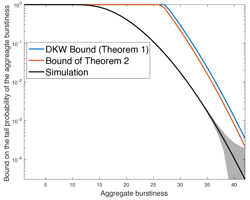
(a)

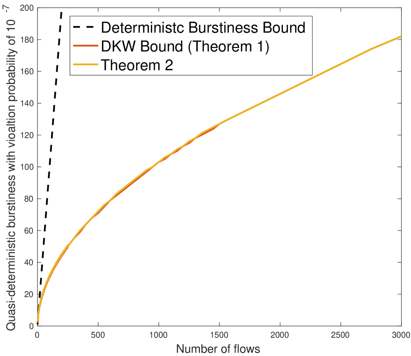
(b)

Figure 1: (a): Bound on the tail probability of the aggregate burstiness obtained by Theorems 4.1, 4.2, and simulations. (b): The obtained quasi-deterministic burstiness with violation probability of $10^{-7}$ by Theorem 4.1 and Theorem 4.2, as the number of flows grows; the deterministic bound (dashed plot) grows linearly with the number of flows.

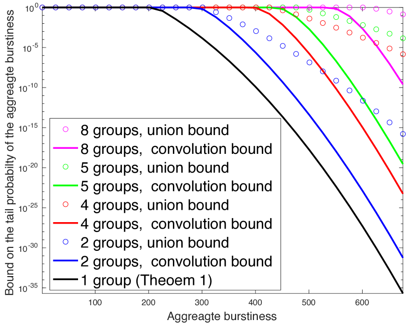
(a)

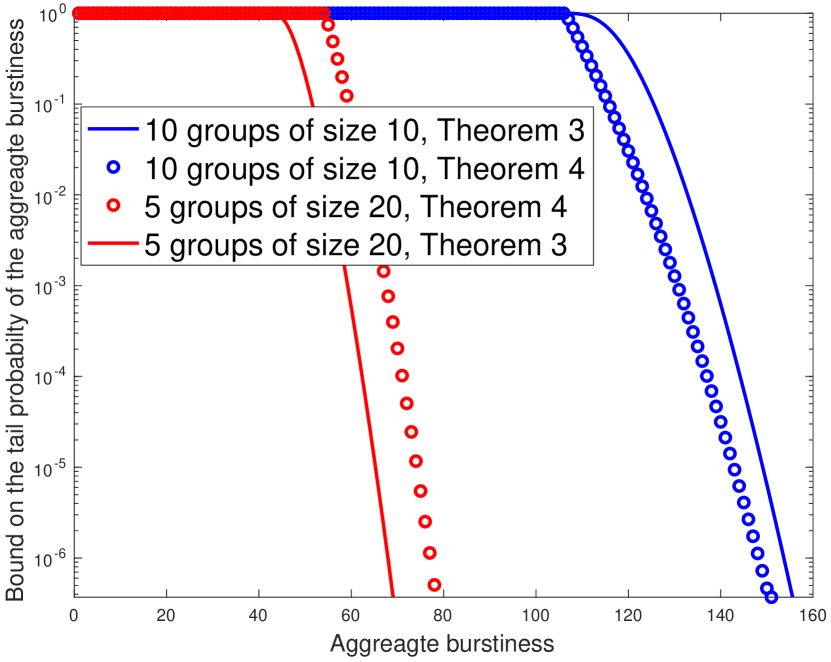
(b)

Figure 2: (a): Comparison of the convolution bound of Theorem 5.1 to the union bound when combining bound obtained for homogeneous sets of flows. (b): Slight improvement of Theorem 5.2 compared to Theorem 5.1 when the number of flows per packet-size is small.

In this section, we numerically illustrate our bounds in Fig. 1 and Fig. 2.

6.1 Homogeneous Case

In Fig. 1(a), we consider $250$ flows with the same packet size (with respect to a unit, is assumed to be $1$) and the same period. We then compute bounds on the tail probability of their aggregate burstiness using Theorems 4.1 and 4.2. We also compute the bound using simulations: For each flow, we independently pick a phase uniformly at random, and we then compute the aggregate burstiness as in (1); we repeat this $10^{8}$ times. We then compute bounds on the tail probability of their aggregate burstiness and its $99\%$ Kolmogorov–Smirnov confidence band. The bound of Theorem 4.2 is slightly better than that of Theorem 4.1. Also, compared to simulations, our bounds are fairly tight.

In Fig. 1(b), we consider $n\in\{2,\ldots,3000\}$ flows with the packet size 1 and same period. We then compute a quasi-deterministic burstiness bound with violation probability of $10^{-7}$ once using Corollary 1 and once using Theorem 4.2; they are almost equal and as $n$ grows are exactly equal, as Theorem 4.1 is as tight as Theorem 4.2 for large $n$. Also, our quasi-deterministic burstiness bound is considerably less than the deterministic one (i.e., $n$) and grows in $\sqrt{n\;\log\;n}$.

6.2 Heterogeneous Case

To assess the efficiency of the bound in the heterogeneous case, we consider in Fig. 2(a) 10000 homogeneous flows with period and packet length 1, and divide them into $g$ groups of $10000/g$ flows, for $g\in\{1,2,4,5,8\}$. We compute a bound for each group by Theorem 4.1, and combine them once with the convolution bound of Theorem 5.1 and once by the union bound (as explained after Proposition 2). Our convolution bound is significantly better than the union bound, and the differences increases fast with the number of sets.

In Fig. 2(b), we consider $10$ (resp. $5$) homogeneous groups of $10$ (resp. $20$) flows, flows of each set $g\in\mathbb{N}_{10}$ (resp. $g\in\mathbb{N}_{5}$), have a packet-size equal to $g$, and all flows have the same period. We then compute the bound on the tail probability of the aggregate burstiness once with Theorem 5.1 and once with Theorem 5.2. When groups are small (here of 10 flows), Theorem 5.2 provides better bounds than Theorem 5.1, but when groups are larger (here of 20 flows), Theorem 5.1 dominates Theorem 5.2.

7 Conclusion

In this paper, we provided quasi-deterministic bounds on the aggregate burstiness for independent, periodic flows. When a small violation tolerance, is allowed, the bounds are considerably better compared to the deterministic bounds. We obtained a closed-form expression for the homogeneous case, and for the heterogeneous case, we combined bounds obtained for homogeneous sets using the convolution bounding technique.

We on purpose limited our study to the burstiness. Quasi-deterministic delay and backlog bounds can be obtained by applying any method from deterministic network calculus, and combining, either by mean of the union bound or (in case of independence) convolution-like manipulations of the burstiness violation events defined for this paper for all groups of flows. Our results can for example be directly applied to [3, Theorem 5], where the model $\textrm{S}^{3}\textrm{BB}$ was used to compute probabilistic delay bounds in tandem networks.

References

- [1] Bouillard, A., Boyer, M., Le Corronc, E.: Deterministic Network Calculus: From Theory to Practical Implementation. Wiley-ISTE (2018)
- [2] Bouillard, A., Nikolaus, P., Schmitt, J.B.: Unleashing the power of paying multiplexing only once in stochastic network calculus. Proc. ACM Meas. Anal. Comput. Syst. 6(2), 31:1–31:27 (2022). https://doi.org/10.1145/3530897, https://doi.org/10.1145/3530897
- [3] Bouillard, A., Nowak, T.: Fast symbolic computation of the worst-case delay in tandem networks and applications. Perform. Eval. 91, 270–285 (2015). https://doi.org/10.1016/j.peva.2015.06.016
- [4] Chang, C.S., Chiu, Y.m., Song, W.T.: On the performance of multiplexing independent regulated inputs. In: Proceedings of the 2001 ACM SIGMETRICS International Conference on Measurement and Modeling of Computer Systems. p. 184–193. SIGMETRICS ’01, Association for Computing Machinery, New York, NY, USA (2001). https://doi.org/10.1145/378420.378782, https://doi.org/10.1145/378420.378782
- [5] Ciucu, F., Burchard, A., Liebeherr, J.: Scaling properties of statistical end-to-end bounds in the network calculus. IEEE/ACM Transactions on Networking (ToN) 14(6), 2300–2312 (2006)
- [6] Ciucu, F., Schmitt, J.: Perspectives on network calculus: No free lunch, but still good value. In: Proceedings of the ACM SIGCOMM 2012 Conference on Applications, Technologies, Architectures, and Protocols for Computer Communication. p. 311–322. SIGCOMM ’12, Association for Computing Machinery, New York, NY, USA (2012). https://doi.org/10.1145/2342356.2342426, https://doi.org/10.1145/2342356.2342426
- [7] Daigmorte, H., Boyer, M.: Traversal time for weakly synchronized can bus. In: Proceedings of the 24th International Conference on Real-Time Networks and Systems. p. 35–44. RTNS ’16, Association for Computing Machinery, New York, NY, USA (2016). https://doi.org/10.1145/2997465.2997477, https://doi.org/10.1145/2997465.2997477
- [8] Fidler, M., Rizk, A.: A guide to the stochastic network calculus. IEEE Communications Surveys & Tutorials 17(1), 92–105 (2015). https://doi.org/10.1109/COMST.2014.2337060
- [9] Gentle, J.: Computational Statistics. Statistics and Computing, Springer New York (2009), https://books.google.ch/books?id=mQ5KAAAAQBAJ
- [10] Guillemin, F.M., Mazumdar, R.R., Rosenberg, C.P., Ying, Y.: A stochastic ordering property for leaky bucket regulated flows in packet networks. Journal of Applied Probability 44(2), 332–348 (2007), http://www.jstor.org/stable/27595845
- [11] Jiang, Y.: A basic stochastic network calculus. In: Proceedings of the 2006 Conference on Applications, Technologies, Architectures, and Protocols for Computer Communications. p. 123–134. SIGCOMM ’06, Association for Computing Machinery, New York, NY, USA (2006). https://doi.org/10.1145/1159913.1159929, https://doi.org/10.1145/1159913.1159929
- [12] Kesidis, G., Konstantopoulos, T.: Worst-case performance of a buffer with independent shaped arrival processes. IEEE Communications Letters 4(1), 26–28 (2000). https://doi.org/10.1109/4234.823539
- [13] Le Boudec, J.Y., Thiran, P.: Network Calculus: A Theory of Deterministic Queuing Systems for the Internet, vol. 2050. Springer Science & Business Media (2001)
- [14] Massart, P.: The Tight Constant in the Dvoretzky-Kiefer-Wolfowitz Inequality. The Annals of Probability 18(3), 1269 – 1283 (1990). https://doi.org/10.1214/aop/1176990746, https://doi.org/10.1214/aop/1176990746
- [15] Poloczek, F., Ciucu, F.: Scheduling analysis with martingales. Performance Evaluation 79, 56 – 72 (2014). https://doi.org/https://doi.org/10.1016/j.peva.2014.07.004, http://www.sciencedirect.com/science/article/pii/S0166531614000674, special Issue: Performance 2014
- [16] Vojnovic, M., Le Boudec, J.Y.: Bounds for independent regulated inputs multiplexed in a service curve network element. In: GLOBECOM’01. IEEE Global Telecommunications Conference (Cat. No.01CH37270). vol. 3, pp. 1857–1861 vol.3 (2001). https://doi.org/10.1109/GLOCOM.2001.965896