IBCL: Zero-shot Model Generation for Task Trade-offs in Continual Learning

Abstract

Like generic multi-task learning, continual learning has the nature of multi-objective optimization, and therefore faces a trade-off between the performance of different tasks. That is, to optimize for the current task distribution, it may need to compromise performance on some previous tasks. This means that there exist multiple models that are Pareto-optimal at different times, each addressing a distinct task performance trade-off. Researchers have discussed how to train particular models to address specific trade-off preferences. However, existing algorithms require training overheads proportional to the number of preferences—a large burden when there are multiple, possibly infinitely many, preferences. As a response, we propose Imprecise Bayesian Continual Learning (IBCL). Upon a new task, IBCL (1) updates a knowledge base in the form of a convex hull of model parameter distributions and (2) obtains particular models to address task trade-off preferences with zero-shot. That is, IBCL does not require any additional training overhead to generate preference-addressing models from its knowledge base. We show that models obtained by IBCL have guarantees in identifying the Pareto optimal parameters. Moreover, experiments on standard image classification and NLP tasks support this guarantee. Statistically, IBCL improves average per-task accuracy by at most 23% and peak per-task accuracy by at most 15% with respect to the baseline methods, with steadily near-zero or positive backward transfer. Most importantly, IBCL significantly reduces the training overhead from training 1 model per preference to at most 3 models for all preferences.

1 Introduction

Multi-task learning inherently solves a multi-objective optimization problem Kendall et al. (2018); Sener and Koltun (2018). This means that the designers face trade-offs between the performance of individual tasks, so they need to select target points on the trade-off curve based on preferences. This situation also applies to a special case of multi-task learning, i.e., lifelong or continual learning, where tasks emerge sequentially from a non-stationary distribution Chen and Liu (2016); Parisi et al. (2019); Ruvolo and Eaton (2013b); Thrun (1998). So far, two major issues remain unresolved in learning models for specific task trade-off points: (1) state-of-the-art algorithms mostly focus on stationary multi-task learning instead of continual learning Lin et al. (2019); Ma et al. (2020), and (2) although a few publications have discussed the continual setting, their methods have to train at least one model per preferred trade-off point. This causes potentially large and unbounded training overhead since there exist infinitely many preferences De Lange et al. (2021); Kim et al. (2023). It would be desirable to efficiently generate models that address specific trade-off preferences with an upper-bounded training overhead, while performance is guaranteed.

Consider two examples: (1) a family television that makes movie recommendations and (2) a single-user computer that is used for a variety of jobs. For the movie recommendation system, each genre (sci-fi, documentaries, etc.) corresponds to a particular task, and the system could train models for making recommendations within each genre. Different family members have different individual viewing preferences over the genres and there are joint preferences for shared viewing. These preferences may even change over time. The television should dynamically switch between these preferences depending on who is viewing, and seamlessly incorporate user feedback, crediting such feedback to the appropriate underlying task and preference models. For the single-user computer, tasks may correspond to particular application configurations, notification settings, etc. Depending on what the user is doing on the computer at a particular time (email, writing, entertainment), there are specific preferences over these configurations/settings that should be active. Feedback should again be credited appropriately to the correct tasks and preferences.

The examples above motivate our problem to reduce training cost upon addressing a large number of preferences. Specifically, our goal is to leverage a small and upper-bounded training overhead per task to address a potentially unbounded number of preferences in continual learning. To the best of our knowledge, this problem is not yet solved by the current state-of-the-art techniques. A typical way of identifying trade-off preference-addressing models in the trade-off Pareto set is to use preference-regularized loss functions Lin et al. (2019; 2020); Kim et al. (2023); Raghavan and Balaprakash (2021), which is expensive due to the need for at least one model being trained per preference. Few-shot meta learning techniques such as MAML Finn et al. (2017) or BMAML Yoon et al. (2018b) are able to generate secondary models from a primary model with small overheads. However, MAML and BMAML do not discuss task trade-off scenarios, and they still require data overhead to train the secondary models. Recall that there exists an unbounded number of preferences, so even if only one data point is required per model, the cost could still be prohibitive. This motivates zero-shot learning techniques. Although existing methods such as hypernetworks enable zero-shot knowledge transfer Von Oswald et al. (2019); Navon et al. (2020), they are not designed for task trade-off preferences and do not guarantee performance.

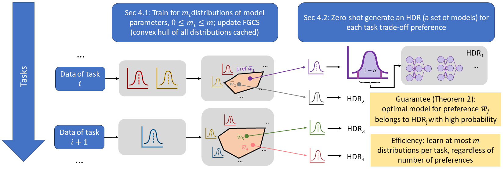
Figure 1: The IBCL workflow. The orange polytopes are the geometric representations of FGCSs.

As a response, we propose Imprecise Bayesian Continual Learning (IBCL), a Bayesian continual learning algorithm that undertakes zero-shot generation of trade-off preference-addressing models with performance guarantees. As shown in Figure 1, IBCL iteratively executes two steps: (1) Upon the arrival of a new task, IBCL updates its knowledge base, which is in the form of a convex hull of model parameter distributions, also known as a finitely generated credal set (FGCS) Caprio et al. (2023). (2) Then, given a user’s preference distribution over all tasks so far, IBCL leverages the knowledge base to zero-shot locate a small set of model parameters. We show that IBCL guarantees the optimal parameter addressing the preference to be in the located parameter set with high confidence. Also, due to step (2) being zero-shot, no additional data or training is needed. Moreover, the overall buffer growth is sublinear in the number of tasks.

Experiments on standard image classification benchmarks – CelebA Liu et al. (2015), Split-CIFAR100 Zenke et al. (2017) and TinyImageNet Le and Yang (2015) – as well as on NLP benchmark 20NewsGroup Lang (1995), show that IBCL is able to outperform baseline preference-addressing methods by at most 23% in average per-task accuracy and 15% in peak per-task accuracy, averaged throughout the tasks. IBCL also shows near zero or positive backward transfer, meaning it is resistant to catastrophic forgetting. Most importantly, it reduces the number of models to be trained per task from the number of preferences per task to a small constant number in $[0,3]$. We also conduct ablation studies to analyze the effect of generating preference-addressing models at different significance levels, as well as different buffer growth speeds.

Contributions. 1. We propose IBCL, a Bayesian continual learning algorithm that (i) guarantees locating the Pareto optimal models that address task trade-off preferences, (ii) zero-shot generates these models with a constant training overhead per task, regardless of number of preferences, and (iii) has a sublinear buffer growth in the number of tasks. 2. We prove IBCL’s optimality probabilistic guarantees. 3. We evaluate IBCL on image classification and NLP benchmarks to support our claims; ablation studies are performed.

2 Related Work

Learning for Pareto-optimal models under task performance trade-offs has been studied by researchers in multi-task learning Caruana (1997); Sener and Koltun (2018). Various techniques have been applied to obtain models that address particular trade-off points Lin et al. (2019; 2020); Ma et al. (2020); Gupta et al. (2021). The idea of preferences on the trade-off points is introduced in multi-objective optimization Lin et al. (2020); Sener and Koltun (2018), and a preference can guide learning algorithms to search for a particular model. We borrow the formalization of preferences from Mahapatra and Rajan (2020), where a preference is given by a vector of non-negative real numbers $\bar{w}$, with each scalar element $w_{i}$ corresponding to task $i$. That is, $w_{i}\geq w_{j}\iff i\succeq j$. This means that if $w_{i}\geq w_{j}$, then task $i$ is preferred to task $j$, and vice versa. However, state-of-the-art algorithms require training one model per preference, imposing large overhead when there is a large number of preferences.

Continual learning, also known as lifelong learning, is a special scenario of multi-task learning, where tasks arrive sequentially instead of simultaneously Thrun (1998); Ruvolo and Eaton (2013a); Silver et al. (2013); Chen and Liu (2016). Algorithms use different mechanisms to transfer knowledge across tasks while avoiding catastrophic forgetting of previously learned knowledge. These include modified loss landscapes for optimization Farajtabar et al. (2020); Kirkpatrick et al. (2017a); Riemer et al. (2019); Suteu and Guo (2019); Tang et al. (2021), preservation of critical pathways via attention Abati et al. (2020); Serra et al. (2018); Xu et al. (2021); Yoon et al. (2020), memory-based methods Lopez-Paz and Ranzato (2017); Rolnick et al. (2019), shared representations He et al. (2018); Lee et al. (2019); Lu et al. (2017); Ruvolo and Eaton (2013b); Vandenhende et al. (2019); Yoon et al. (2018a), and dynamic representations Bulat et al. (2020); Mendez and Eaton (2021); Ramesh and Chaudhari (2022); Rusu et al. (2016); Schwarz et al. (2018); Yang and Hospedales (2017). Bayesian, or probabilistic methods such as variational inference are also adopted Ebrahimi et al. (2019); Farquhar and Gal (2019); Kao et al. (2021); Kessler et al. (2023); Li et al. (2020); Nguyen et al. (2018). We collectively refer to all information shared across tasks as a knowledge base. In this paper, we leverage Bayesian inference in the knowledge base update. We discuss the reason for working in a Bayesian continual learning setting in Appendix B.

Like generic multi-task learning, continual learning also faces trade-off between tasks, known as the stability-plasticity trade-off De Lange et al. (2021); Kim et al. (2023); Raghavan and Balaprakash (2021), which balances between performance on new tasks and resistance to catastrophic forgetting Kirkpatrick et al. (2017b); Lee et al. (2017); Robins (1995). Current methods identify models to address trade-off preferences by techniques such as loss regularization Servia-Rodriguez et al. (2021), meaning at least one model needs to be trained per preference.

Finally, our algorithm hinges upon concepts from Imprecise Probability (IP) theory Walley (1991); Troffaes and de Cooman (2014); Caprio and Gong (2023); Caprio and Mukherjee (2023); Caprio and Seidenfeld (2023); Caprio et al. (2023). Specifically, we use the concept of finitely generated credal set (FGCS), which is defined as follows.

Definition 1 (Finitely Generated Credal Set).

A convex set $\mathcal{Q}=\{Q:Q=\sum_{j=1}^{m}\beta^{j}Q^{j}\text{, }\beta_{j}\geq 0\text{ }\forall j\text{, }\sum_{j}\beta_{j}=1\}$ of probability distributions with finitely many extreme elements is called a finitely generated credal set (FGCS).

In other words, an FGCS is a convex hull of distributions. We denote the extreme elements of an FGCS $\mathcal{Q}$ by $\text{ex}[\mathcal{Q}]=\{Q^{j}\}_{j=1}^{m}$. We also borrow from the Bayesian literature the idea of highest density region (HDR). Consider a generic probability measure $Q$ defined on some space $\Theta$ having pdf/pmf $q$, and pick any significance level $\alpha\in[0,1]$.

Definition 2 (Highest Density Region Hyndman (1996)).

The $\alpha$-level Highest Density Region (HDR) $R_{\alpha}(Q)$ is the subset of $\Theta$ defined as $R_{\alpha}(Q):=\{\theta\in\Theta:q(\theta)\geq{q}^{\alpha}\}$, where ${q}^{\alpha}$ is a constant value. In particular, it is the largest constant such that $\text{Pr}_{Q}[\theta\in R_{\alpha}(Q)]\geq 1-\alpha$.

In other words, an HDR $R_{\alpha}(Q)$ is the smallest subset of $\Theta$ that is needed to guarantee a probability of at least $1-\alpha$ according to $Q$. The concept of HDR is further explored in Appendix C.

3 Problem Formulation

Our goal is to obtain Bayesian classification models that accurately and flexibly express user-specified preferences over all encountered tasks throughout domain incremental learning. The procedure must guarantee optimality when computing a model that addresses a preference. Moreover, its sample complexity should not scale up with the number of user preferences.

Formally, we denote by $(\cdot,\mathcal{A}_{\cdot})$ the pair of a set and a $\sigma$-algebra endowed to it, i.e., a measurable space. Let $(\mathcal{X},\mathcal{A}_{\mathcal{X}})$ be the measurable space of data, $(\mathcal{Y},\mathcal{A}_{\mathcal{Y}})$ be the measurable space of labels, and $(\mathcal{X}\times\mathcal{Y},\mathcal{A}_{\mathcal{X}\times\mathcal{Y}})$ be the measurable product space of data and labels. Next, we denote by $\Delta(\cdot,\mathcal{A}_{\cdot})$ the space of all probability measures on the corresponding measurable space. Hence, $\Delta_{\mathcal{XY}}\equiv\Delta(\mathcal{X}\times\mathcal{Y},\mathcal{A}_{\mathcal{X}\times\mathcal{Y}})$ indicates the distribution space over all labeled data, and $\Delta_{\Theta}\equiv\Delta(\Theta,\mathcal{A}_{\Theta})$ is the space of distributions over the parameter space $\Theta$, for some $\sigma$-algebra $\mathcal{A}_{\Theta}$ endowed to $\Theta$.

Throughout the domain incremental learning process, each task $i$ is associated with an unknown underlying distribution $P_{i}\in\Delta_{\mathcal{X}\mathcal{Y}}$. We assume that all tasks are similar to each other. We formalize this statement as follows.

Assumption 1 (Task Similarity).

For all task $i$, $P_{i}\in\mathcal{F}$, where $\mathcal{F}$ is a convex subset of $\Delta_{\mathcal{XY}}$. Also, we assume that the diameter of $\mathcal{F}$ is some $r>0$, that is, $\sup_{F,F^{\prime}\in\mathcal{F}}\|F-F^{\prime}\|_{W_{2}}\leq r$, where $\|\cdot\|_{W_{2}}$ denotes the $2$-Wasserstein distance.

In an effort to make the paper self-contained, in Appendix D we give the definition of $2$-Wasserstein distance. Under Assumption 1, for any two tasks $i$ and $j$, their underlying distributions $P_{i}$ and $P_{j}$ satisfy $\|P_{i}-P_{j}\|_{W_{2}}\leq r$. Moreover, since $\mathcal{F}$ is convex, any convex combination of task distributions belongs to $\mathcal{F}$. The importance of Assumption 1 is discussed in Appendix E. Next, we assume the parameterization. An example of a parametrized family $\mathcal{F}$ is given in Appendix F.

Assumption 2 (Parameterization).

Every distribution $F$ in $\mathcal{F}$ is parametrized by $\theta$, a parameter belonging to a parameter space $\Theta$.

We then formalize preferences over tasks; see Appendix G for more.

Definition 3 (Preferences).

Consider $k$ tasks with underlying distributions $P_{1},P_{2},\dots,P_{k}$. We express a preference over them via a probability vector $\bar{w}=(w_{1},w_{2},\dots,w_{k})^{\top}$, that is, $w_{j}\geq 0$ for all $j\in\{1,\ldots,k\}$, and $\sum_{j=1}^{k}w_{j}=1$.

Based on this definition, given a preference $\bar{w}$ over all $k$ tasks encountered, an object of interest is $P_{\bar{w}}:=\sum_{i=1}^{k}w_{i}P_{i}$, or in dot product form $P_{\bar{w}}:=\bar{w}\cdot\bar{P}$, where $\bar{P}=(P_{1},\ldots,P_{k})^{\top}$. It is the distribution associated with tasks $1,\ldots,k$ that also takes into account a preference over them. Under Assumptions 1 and 2, we have that $P_{\bar{w}}\in\mathcal{F}$, and therefore it is also parameterized by some $\theta\in\Theta$.

The learning procedure is the same as conventional supervised domain-incremental learning. That is, upon task $i$, we draw $n_{i}$ labeled examples i.i.d. from an unknown $P_{i}$ on $\mathcal{X}\times\mathcal{Y}$. In addition, we are given at least one preference in the form of $\bar{w}$ over the $i$ tasks encountered so far. The data drawn for task $i+1$ will not be available until we have finished learning all preference-addressing models at task $i$. Our goal is to find the correct parameter (i.e., the optimal model) $\theta_{\bar{w}}^{\star}$ for each $P_{\bar{w}}$ as follows.

Main Problem. Suppose that we have encountered $k\geq 1$ tasks so far. On the domain-incremental learning procedure described above, given a significance level $\alpha\in[0,1]$, we want to design an algorithm that satisfies the following properties.

1. Preference addressing guarantee. Given a preference $\bar{w}$, we want to identify a distribution $\hat{Q}_{\bar{w}}$ on $\Theta$ that assigns probability of at least $1-\alpha$ to the event $\theta_{\bar{w}}^{\star}\in R_{\alpha}(\hat{Q}_{\bar{w}})$, where $R_{\alpha}(\hat{Q}_{\bar{w}})\subset\Theta$ is an HDR as in Definition 2.

2. Zero-shot preference adaptation. After obtaining the parameter HDR for a preference $\bar{w}$, locating the HDR for any number of new preferences at the current task does not cost additional training data. Locating each new HDR must also satisfy the preference addressing guarantee.

3. Sublinear buffer growth. The memory overhead for the entire procedure should be growing sublinearly in the number of tasks.

In the next section we present the Imprecise Bayesian Continual Learning (IBCL) procedure, together with its associated algorithm, that tackles the main problem.

4 Imprecise Bayesian Continual Learning

4.1 FGCS Knowledge Base Update

We take a Bayesian continual learning approach to solve the main problem above; that is, model parameters are viewed as random variables. However, unlike the existing Bayesian continual learning literature Kao et al. (2021); Lee et al. (2017); Li et al. (2020), we take into account the ambiguity faced by the agent in eliciting the probability model. Specifically, instead of maintaining one distribution of parameters as the knowledge base, we iteratively update an FGCS of parameter distributions. Our knowledge base stores its extreme points.

Formally, to distinguish from a labeled data distribution $P\in\Delta_{\mathcal{XY}}$, we denote parameter distributions by $Q\in\Delta_{\Theta}$. Also, we denote a likelihood by $L\in\Delta_{\mathcal{XY}}$. The product of likelihoods up to task $i$ is an estimation of the ground-truth $P_{i}$ based on observed data. The pdf/pmf of a distribution is denoted by lower-case letters, i.e., $q$ for $Q$, $l$ for $L$, etc.

Algorithm 1 FGCS Knowledge Base Update

Input: Current knowledge base in the form of FGCS extreme elements (prior set)
      $\text{ex}[\mathcal{Q}^{\text{co}}_{i-1}]=\{Q^{1}_{i-1},\dots,Q^{m}_{i-1}\}$, observed labeled data $(\bar{x}_{i},\bar{y}_{i})$ accruing to task $i$, and distribution difference threshold $d\geq 0$
      Output: Updated extreme elements (posterior set) $\text{ex}[\mathcal{Q}^{\text{co}}_{i}]$

1:$\mathcal{Q}_{i}\leftarrow\emptyset$

2:$L_{i}\leftarrow L((\bar{x}_{i},\bar{y}_{i})\mid\theta)$

3:for $j\in\{1,\dots,m\}$ do

4:     $q_{i}^{j}\leftarrow\frac{q_{i-1}^{j}(\theta)\times l_{i}(x_{1_{i}},y_{1_{i}},\ldots,x_{n_{i}},y_{n_{i}}\mid\theta)}{\int_{\Theta}q_{i-1}^{j}(\theta)\times l_{i}(x_{1_{i}},y_{1_{i}},\ldots,x_{n_{i}},y_{n_{i}}\mid\theta)\text{ d}\theta}$ $\triangleright$ % Approximate via variational inference

5:     $d_{i}^{j}\leftarrow\min_{Q\in\text{ex}[\mathcal{Q}^{\text{co}}_{i-1}]}\|Q_{i}^{j}-Q\|_{W_{2}}$

6:     if $d_{i}^{j}\geq d$ then

7:         $\mathcal{Q}_{i}\leftarrow\mathcal{Q}_{i}\cup\{Q_{i}^{j}\}$

8:     else

9:         Remember to use $Q=\arg\min_{Q\in\text{ex}[\mathcal{Q}^{\text{co}}_{i-1}]}\|Q_{i}^{j}-Q\|_{W_{2}}$ in place of $Q_{i}^{j}$ later on.

10:     end if

11:end for

12:$\text{ex}[\mathcal{Q}^{\text{co}}_{i}]\leftarrow\text{ex}[\mathcal{Q}^{\text{co}}_{i-1}]\cup\mathcal{Q}_{i}$

We denote the FGCS at task $i$ by $\mathcal{Q}^{\text{co}}_{i}$, where “co” stands for “convex hull”. Upon task $i$, we observe $n_{i}$ labeled data points. In Algorithm 1, we maintain and update a knowledge base of the FGCS extreme points, i.e., the set $\text{ex}[\mathcal{Q}^{\text{co}}_{i}]$. This because any $Q\in\mathcal{Q}^{\text{co}}_{i}$ can be written as a convex combination of the elements in $\text{ex}[\mathcal{Q}^{\text{co}}_{i}]$. Notice that we have $m$ different priors $Q^{1}_{i-1},\cdots,Q^{m}_{i-1}$ resulting from previous task $i-1$. This procedure learns $m$ posteriors $Q^{1}_{i},\dots,Q^{m}_{i}$ respectively from the priors by Bayesian inference, which is implemented using variational techniques. In line 2, we define a likelihood function based on the observed data and on parameter $\theta$ (this latter, since we are in a Bayesian setting, is a random variable). Next, in lines 4 and 5, we compute the $m$ posteriors from their corresponding priors one-by-one, together with their distance from $\text{ex}[\mathcal{Q}^{\text{co}}_{i-1}]$.

Learning $m$ posteriors does not necessarily mean that we want to buffer all of them in the knowledge base. In lines 6-10, we check – using the distance from $\text{ex}[\mathcal{Q}^{\text{co}}_{i-1}]$ – whether there already exists a sufficiently similar distribution $Q\in\text{ex}[\mathcal{Q}^{\text{co}}_{i-1}]$ to the newly learned $Q_{i}^{j}$. If so, we do not buffer the new posterior but remember to use $Q$ in place of $Q_{i}^{j}$ from now on. The similarity is measured via the 2-Wasserstein distance Deza and Deza (2013). In practice, when all distributions are modeled by Bayesian neural networks with independent normal weights and biases, we have

$$\|Q_{1}-Q_{2}\|^{2}_{W_{2}}=\|\mu_{Q_{1}}^{2}-\mu_{Q_{2}}^{2}\|_{2}^{2}+\|\sigma_{Q_{1}}^{2}\mathbf{1}-\sigma_{Q_{2}}^{2}\mathbf{1}\|_{2}^{2},$$ (1)

where $\|\cdot\|_{2}$ denotes the Euclidean norm, $\mathbf{1}$ is a vector of all $1$’s, and $\mu_{Q}$ and $\sigma_{Q}$ are respectively the mean and standard deviation of a multivariate normal distribution $Q$ with independent dimensions, $Q=\mathcal{N}(\mu_{Q},\sigma^{2}_{Q}I)$, $I$ being the identity matrix. Notice that this replacement ensures sublinear buffer growth in our problem formulation, because at each task $i$ we only buffer $m_{i}$ new posterior models, with $0\leq m_{i}\leq m$. With sufficiently large threshold $d$, the buffer growth can become constant after several tasks. The choice of $d$ can be estimated by computing pairwise 2-Wasserstein distances in the FGCS and then take the $0.1$-quantile. Our ablation study in Appendix J shows the effect of different choices of $d$.

Finally, in line 12, the posteriors are appended to the FGCS extreme points to update the knowledge base.

4.2 Zero-shot Preference Adaptation from Knowledge Base

Next, after we update the FGCS extreme points for task $i$, we are given a set of user preferences. For each preference $\bar{w}$, we need to identify the optimal parameter $\theta^{\star}_{\bar{w}}$ for the preferred data distribution $P_{\bar{w}}$. This procedure can be divided into two steps as follows.

First, we compute distribution $\hat{Q}_{\bar{w}}$ based on the knowledge base and the preference. Here, the knowledge base consists of the extreme points of a convex set, and we decide the convex combination weights based on the preferences. That is,

$$\hat{Q}_{\bar{w}}=\sum_{k=1}^{i}\sum_{j=1}^{m_{k}}\beta_{k}^{j}Q_{k}^{j},\quad\text{where }\sum_{j=1}^{m_{k}}\beta_{k}^{j}=w_{k}\text{, and }\beta_{k}^{j}\geq 0,\text{ for all }j\text{ and all }k.$$ (2)

Here, $Q_{k}^{j}$ is an extreme point of FGCS $\mathcal{Q}^{\text{co}}_{k}$, i.e. the $j$-th parameter posterior of task $k$. The weight $\beta_{k}^{j}$ of each extreme point is decided by preference $\bar{w}$. In implementation, if we have $m_{k}$ extreme points stored for task $k$, we can choose equal weights $\beta_{k}^{1}=\dots=\beta_{k}^{m}=w_{k}/m_{k}$. For example, if we have preference $\bar{w}=(0.8,0.2)$ on two tasks so far, and we have two extreme points per task stored in the knowledge base, we can use $\beta_{1}^{1}=\beta_{1}^{2}=0.8/2=0.4$ and $\beta_{2}^{1}=\beta_{2}^{2}=0.2/2=0.1$.

Second, we compute the HDR $R_{\alpha}(\hat{Q}_{\bar{w}})\subset\Theta$ from $\hat{Q}_{\bar{w}}$. This is implemented via a standard procedure that locates a region in the parameter space whose enclosed probability mass is (at least) $1-\alpha$, according to $\hat{Q}_{\bar{w}}$. This procedure can be routinely implemented, e.g., in R, using package HDInterval Juat et al. (2022). As a result, we locate a set of parameters $R_{\alpha}(\hat{Q}_{\bar{w}})$ associated with the preference $\bar{w}$. This subroutine is formalized in Algorithm 2, and one remark is that it does not require any training data, i.e., we identify a set of parameters by zero-shot preference adaptation. This meets our goal in the main problem.

Algorithm 2 Preference HDR Computation

Input: Knowledge base $\text{ex}[\mathcal{Q}^{\text{co}}_{i}]$ with $m_{k}$ extreme points saved for task $k$,
      preference vector $\bar{w}$ on the $i$ tasks, significance level $\alpha\in[0,1]$
      Output: HDR $R_{\alpha}(\hat{Q}_{\bar{w}})\subset\Theta$

1:for $k=1,\dots,i$ do

2:     $\beta_{k}^{1}=\dots=\beta_{k}^{m}\leftarrow w_{k}/m_{k}$

3:end for

4:$\hat{Q}_{\bar{w}}=\sum_{k=1}^{i}\sum_{j=1}^{m_{k}}\beta_{k}^{j}Q_{k}^{j}$

5:$R_{\alpha}(\hat{Q}_{\bar{w}})\leftarrow hdr(\hat{Q}_{\bar{w}},\alpha)$

4.3 Overall IBCL Algorithm and Analysis

From the two subroutines in Sections 4.1 and 4.2, we construct the overall IBCL algorithm as in Algorithm 3.

Algorithm 3 Imprecise Bayesian Continual Learning

Input: Prior distributions $\text{ex}[\mathcal{Q}^{\text{co}}_{0}]=\{Q^{1}_{0},\dots,Q^{m}_{0}\}$, hyperparameters $\alpha$ and $d$
      Output: HDR $R_{\alpha}(\hat{Q}_{\bar{w}})$ for each given preference $\bar{w}$ at each task $i$

1:for task $i=1,2,...$ do

2:     $\bar{x}_{i},\bar{y}_{i}\leftarrow$ sample $n_{i}$ labeled data points i.i.d. from $P_{i}$

3:     $\text{ex}[\mathcal{Q}^{\text{co}}_{i}]\leftarrow fgcs\_knowledge\_base\_update(\text{ex}[\mathcal{Q}^{\text{co}}_{i-1}],\bar{x}_{i},\bar{y}_{i},d)$

4:     while user has a new preference do

5:         $\bar{w},\alpha\leftarrow$ user input

6:         $R_{\alpha}(\hat{Q}_{i})\leftarrow preference\_hdr\_computation(\text{ex}[\mathcal{Q}^{\text{co}}_{i}],\bar{w},\alpha)$

7:     end while

8:end for

For each task, in line 3, we use Algorithm 1 to update the knowledge base by learning $m$ posteriors from the current priors. Some of these posteriors will be cached and some will be substituted by a previous distribution in the knowledge base. In lines 4-6, upon a user-given preference over all tasks so far, we obtain the HDR of the model associated with preference $\bar{w}$ with zero-shot via Algorithm 2. Notice that this HDR computation does not require the initial priors $\text{ex}[\mathcal{Q}_{0}^{\text{co}}]$, so we can discard them once the posteriors are learned in the first task. The following theorems assure that IBCL solves the main problem in Section 3.

Theorem 1 (Selection Equivalence).

Selecting a precise distribution $\hat{Q}_{\bar{w}}$ from $\mathcal{Q}^{\text{co}}_{i}$ is equivalent to specifying a preference weight vector $\bar{w}$ on $P_{1},\dots,P_{i}$.

Theorem 1 entails that the selection of $\hat{Q}_{\bar{w}}$ in Algorithm 2 is related to the correct parametrization of $P_{\bar{w}}\in\Delta_{\mathcal{XY}}$. We also have the following.

Theorem 2 (Optimality Guarantee).

Pick any $\alpha\in[0,1]$. The correct parameter $\theta_{\bar{w}}^{\star}$ for $P_{\bar{w}}$ belongs to $R_{\alpha}(\hat{Q}_{\bar{w}})$ with probability at least $1-\alpha$, according to $\hat{Q}_{\bar{w}}$. In formulas,

$$\text{Pr}_{\hat{Q}_{\bar{w}}}\left[\theta^{\star}_{\bar{w}}\in R_{\alpha}(\hat{Q}_{\bar{w}})\right]\geq 1-\alpha.$$ (3)

From Theorem 2 we see a $(1-\alpha)$-guarantee in obtaining Pareto-optimal models for given task trade-off preferences. Consequently, the IBCL algorithm enjoys the preference addressing guarantee targeted by our main problem. Theorems 1 and 2 are both proven in Appendix H.

5 Experiments

5.1 Setup

We experiment IBCL on four domain-incremental learning benchmarks, inclduing three image classifications and one NLP/text classification. The benchmarks include: (1) 15 tasks from CelebA Liu et al. (2015). For each task we classify whether a celebrity face has an attribute or not, such as wearing glasses. (2) 10 tasks from Split-CIFAR100 Zenke et al. (2017). For each task we classify a type of animal vs. a type of non-animal, such as beaver vs. bus and dolphin vs. lawn mower. (3) 10 tasks from TinyImageNet Le and Yang (2015), also on animals vs. non-animals. (4) 5 tasks from 20NewsGroup Lang (1995). For each task we classify whether a news report is on a computer-related topic, such as computer graphics vs. sales and computer OS vs. automobiles. In preprocessing, we extract features of the three image benchmarks by a pre-trained ResNet-18 He et al. (2016), and 20NewsGroup by a TF-IDF vectorizer Aizawa (2003).

We compare IBCL to the following four baseline methods.

1. Gradient Episodic Memory (GEM). GEM trains one deterministic model per task, using current task’s training data as well as a constant number of data memorized per previous task Lopez-Paz and Ranzato (2017).

2. Preference-regularized GEM (GEM-reg). This method trains multiple GEM models, one per preference, at each task. Each model is trained by a loss function regularized by a preference De Lange et al. (2021); Lin et al. (2020; 2019).

3. Variational Continual Learning (VCL). VCL leverages Bayesian models to learn one probabilistic model per task. The same memorization of previous training data as in GEM is also applied to VCL Nguyen et al. (2018).

4. Preference-regularized VCL (VCL-reg). Similar to GEM-reg, this method trains multiple probabilistic models per task, one per preference. Each model’s loss function is regularized by a preference Servia-Rodriguez et al. (2021).

Overall, GEM and VCL are efficient, because they train only one model per task, but they do not address task trade-off preferences. GEM-reg and VCL-reg address preferences but require training multiple models (one model per preference), lowering the efficiency. All model architecture and hyperparameters (learning rate, batch sizes and epochs) are kept the same for IBCL and baselines. At each task, we randomly generate $K=10$ preferences, which means GEM-reg, VCL-reg and IBCL need to produce $K$ preference-addressing models, while GEM and VCL produce 1 model to address all preferences.

We evaluate an algorithm’s performance using continual learning metrics, i.e., average per-task accuracy and peak per-task accuracy. We also measure backward transfer Díaz-Rodríguez et al. (2018) for resistance to catastrophic forgetting. For probabilistic methods (VCL, VCL-reg and IBCL), we sample $100$ deterministic models from each probabilistic models and record their max, mean and min value on the metrics. The max value will be the estimated Pareto performance. Experiments run on a PC equipped with Intel(R) Core(TM) i7-8550U CPU @ 1.80GHz. More setup details can be found in Appendix I.

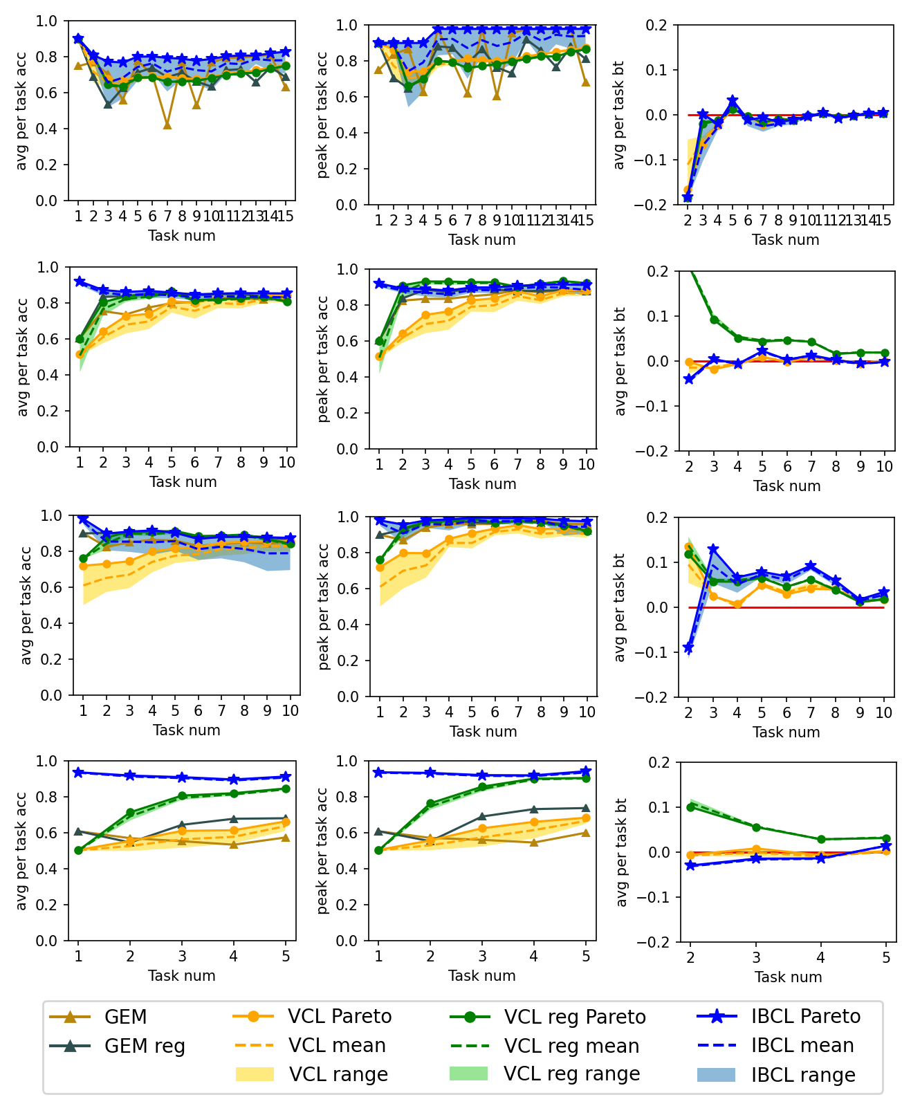
Figure 2: Top to bottom: Results on CelebA, Split-CIFAR100, TinyImageNet and 20NewsGroup.

5.2 Main Results

As shown in Figure 2, the Pareto optimality identified by IBCL outperforms the baselines in both average per-task accuracy and peak per-task accuracy. The largest disparity between IBCL and baselines appears in the 20NewsGroup benchmark, where the average per-task accuracy and peak per-task accuracy of IBCL improve on VCL-reg’s Pareto solutions by 23% and 15%, respectively, when averaged across the tasks. This performance supports our preference-addressing guarantee in Theorem 2. Moreover, IBCL’s backward transfer is steadily around 0 or positive, meaning that its performance on previous tasks is either maintained or enhanced after new training is done. This implies that IBCL is resistant to catastrophic forgetting. Notice that the main results are produced with $\alpha=0.01$ and $d=0.002$ on all benchmarks. They are selected based on performance on a hold-out validation set. We discuss ablation studies on $\alpha$ and $d$ in Appendix J.

Table 1: Overhead comparison between IBCL and baselines. Please refer to the ablation studies in Appendix J for the detailed number of models trained by IBCL.

Method	Num Models Trained per Task	Additional Overhead	Pref-addressing
GEM	1	mem of previous data	no
GEM-reg	$10$ (num of preferences)		yes
VCL	1		no
VCL-reg	$10$ (num of preferences)		yes
IBCL (ours)	$\leq 3$	N/A	yes

Overall, compared to the baselines, we show that IBCL not only achieves similar to better performance in addressing task trade-off preferences in continual learning, but also significantly reduces the training overhead. We also conduct ablation studies on different $\alpha$ and $d$; the results are discussed in Appendix J.

6 Discussion and Conclusion

Advantages of IBCL. The most significant advantage is its zero-shot preference addressing. No matter how many different task trade-off preferences need to be addressed, IBCL only requires a constant training overhead per task for the FGCS update. Also, by using IBCL, the model that addresses one preference is not affected by previous models that address different preferences, because all models are independently derived from the same FGCS. Moreover, the identified parameter HDRs have a $(1-\alpha)$-guarantee of containing the optimum.

Limitations of IBCL. As shown in the experiments, poorly performing models can also be sampled from IBCL’s HDRs. However, in practice, we can sample a finite number of models, such as 100 models per HDR as in the experiments, and check their performance on a validation set. Because validation data points are drawn from the same data generation process, sampled models with high validation results are likely to be close to the actual Pareto front.

Overall, we propose a probabilistic continual learning algorithm, namely IBCL, to locate models that address particular task trade-off preferences. Theoretically and empirically, we show that IBCL is able to locate models that address different user-given preferences via zero-shot at each task, with guaranteed performance. This means the training overhead does not scale up with the number of preferences, significantly reducing the computational cost.

Appendix A Relationship between IBCL and MAML

In this section, we discuss the relationship between IBCL and the Model-Agnostic Meta-Learning (MAML) and Bayesian MAML (BMAML) procedures introduced in Finn et al. [2017], Yoon et al. [2018b], respectively. These are inherently different than IBCL, since the latter is a continual learning procedure, while MAML and BMAML are meta-learning algorithms. Nevertheless, given the popularity of these procedures, we feel that relating IBCL to them would be useful to draw some insights on IBCL itself.

In MAML and BMAML, a task $i$ is specified by a $n_{i}$-shot dataset $D_{i}$ that consists of a small number of training examples, e.g. observations $(x_{1_{i}},y_{1_{i}}),\ldots,(x_{n_{i}},y_{n_{i}})$. Tasks are sampled from a task distribution $\mathbb{T}$ such that the sampled tasks share the statistical regularity of the task distribution. In IBCL, Assumption 1 guarantees that the tasks $P_{i}$ share the statistical regularity of class $\mathcal{F}$. MAML and BMAML leverage this regularity to improve the learning efficiency of subsequent tasks.

At each meta-iteration $i$,

1. Task-Sampling: For both MAML and BMAML, a mini-batch $T_{i}$ of tasks is sampled from the task distribution $\mathbb{T}$. Each task $\tau_{i}\in T_{i}$ provides task-train and task-validation data, $D^{\text{trn}}_{\tau_{i}}$ and $D^{\text{val}}_{\tau_{i}}$, respectively.

2. Inner-Update: For MAML, the parameter of each task $\tau_{i}\in T_{i}$ is updated starting from the current generic initial parameter $\theta_{0}$, and then performing $n_{i}$ gradient descent steps on the task-train loss. For BMAML, the posterior $p(\theta_{\tau_{i}}\mid D^{\text{trn}}_{\tau_{i}},\theta_{0})$ is computed, for all $\tau_{i}\in T_{i}$.

3. Outer-Update: For MAML, the generic initial parameter $\theta_{0}$ is updated by gradient descent. For BMAML, it is updated using the Chaser loss [Yoon et al., 2018b, Equation (7)].

Notice how in our work $\bar{w}$ is a probability vector. This implies that if we fix a number of task $k$ and we let $\bar{w}$ be equal to $(w_{1},\ldots,w_{k})^{\top}$, then $\bar{w}\cdot\bar{P}$ can be seen as a sample from $\mathbb{T}$ such that $\mathbb{T}(P_{i})=w_{i}$, for all $i\in\{1,\ldots,k\}$.

Here lies the main difference between IBCL and BMAML. In the latter the information provided by the tasks is used to obtain a refinement of the (parameter of the) distribution $\mathbb{T}$ on the tasks themselves. In IBCL, instead, we are interested in the optimal parametrization of the posterior distribution associated with $\bar{w}\cdot\bar{P}$. Notice also that at time $k+1$, in IBCL the support of $\mathbb{T}$ changes: it is $\{P_{1},\ldots,P_{k+1}\}$, while for MAML and BMAML it stays the same.

Also, MAML and BMAML can be seen as ensemble methods, since they use different values (MAML) or different distributions (BMAML) to perform the Outer-Update and come up with a single value (MAML) or a single distributions (BMAML). Instead, IBCL keeps distributions separate via FGCS, thus capturing the ambiguity faced by the designer during the analysis.

Furthermore, we want to point out how while for BMAML the tasks $\tau_{i}$ are all “candidates” for the true data generating process (dgp) $P_{i}$, in IBCL we approximate $P_{i}$ with the product $\prod_{h=1}^{i}L_{h}$ of the likelihoods up to task $i$. The idea of different candidates for the true dgp is beneficial for IBCL as well: in the future, we plan to let go of Assumption 1 and let each $P_{i}$ belong to a credal set $\mathcal{P}_{i}$. This would capture the epistemic uncertainty faced by the agent on the true dgp.

To summarize, IBCL is a continual learning technique whose aim is to find the correct parametrization of the posterior associated with $\bar{w}\cdot\bar{P}$. Here, $\bar{w}$ expresses the developer’s preferences on the tasks. MAML and BMAML, instead, are meta-learning algorithms whose main concern is to refine the distribution $\mathbb{T}$ from which the tasks are sampled. While IBCL is able to capture the preferences of, and the ambiguity faced by, the designer, MAML and BMAML are unable to do so. On the contrary, these latter seem better suited to solve meta-learning problems. An interesting future research direction is to come up with imprecise BMAML, or IBMAML, where a credal set $\text{Conv}(\{\mathbb{T}_{1},\ldots,\mathbb{T}_{k}\})$ is used to capture the ambiguity faced by the developer in specifying the correct distribution on the possible tasks. The process of selecting one element from such credal set may lead to computational gains.

Appendix B Reason to use Bayesian continual learning

Let $q_{0}(\theta)$ be our prior pdf/pmf on parameter $\theta\in\Theta$ at time $t=0$. At time $t=1$, we collect data $(\bar{x}_{1},\bar{y}_{1})$ pertaining to task $1$, we elicit likelihood pdf/pmf $l_{1}(\bar{x}_{1},\bar{y}_{1}\mid\theta)$, and we compute $q_{1}(\theta\mid\bar{x}_{1},\bar{y}_{1})\propto q_{0}(\theta)\times l_{1}(\bar{x}_{1},\bar{y}_{1}\mid\theta)$. At time $t=2$, we collect data $(\bar{x}_{2},\bar{y}_{2})$ pertaining to task $2$ and we elicit likelihood pdf/pmf $l_{2}(\bar{x}_{2},\bar{y}_{2}\mid\theta)$. Now we have two options.

• Bayesian Continual Learning (BCL): we let the prior pdf/pmf at time $t=2$ be the posterior pdf/pmf at time $t=1$. That is, our prior pdf/pmf is $q_{1}(\theta\mid\bar{x}_{1},\bar{y}_{1})$, and we compute $q_{2}(\theta\mid\bar{x}_{1},\bar{y}_{1},\bar{x}_{2},\bar{y}_{2})\propto q_{1}(\theta\mid\bar{x}_{1},\bar{y}_{1})\times l_{2}(\bar{x}_{2},\bar{y}_{2}\mid\theta)\propto q_{0}(\theta)\times l_{1}(\bar{x}_{1},\bar{y}_{1}\mid\theta)\times l_{2}(\bar{x}_{2},\bar{y}_{2}\mid\theta)$;

• Bayesian Isolated Learning (BIL): we let the prior pdf/pmf at time $t=2$ be a generic prior pdf/pmf $q_{0}^{\prime}(\theta)$. We compute $q_{2}^{\prime}(\theta\mid\bar{x}_{2},\bar{y}_{2})\propto q_{0}^{\prime}(\theta)\times l_{2}(\bar{x}_{2},\bar{y}_{2}\mid\theta)$. We can even re-use the original prior, so that $q_{0}^{\prime}=q_{0}$.

As we can see, in option (i) we assume that the data generating process at time $t=2$ takes into account both tasks, while in option (ii) we posit that it only takes into account task $2$. Denote by $\sigma(X)$ the sigma-algebra generated by a generic random variable $X$. Let also $Q_{2}$ be the probability measure whose pdf/pmf is $q_{2}$, and $Q_{2}^{\prime}$ be the probability measure whose pdf/pmf is $q_{2}^{\prime}$. Then, we have the following.

Proposition 3.

Posterior probability measure $Q_{2}$ can be written as a $\sigma(\bar{X}_{1},\bar{Y}_{1},\bar{X}_{2},\bar{Y}_{2})$-measurable random variable taking values in $[0,1]$, while posterior probability measure $Q_{2}^{\prime}$ can be written as a $\sigma(\bar{X}_{2},\bar{Y}_{2})$-measurable random variable taking values in $[0,1]$.

Proof.

Pick any $A\subset\Theta$. Then, $Q_{2}[A\mid\sigma(\bar{X}_{1},\bar{Y}_{1},\bar{X}_{2},\bar{Y}_{2})]=\mathbb{E}_{Q_{2}}[\mathbbm{1}_{A}\mid\sigma(\bar{X}_{1},\bar{Y}_{1},\bar{X}_{2},\bar{Y}_{2})]$, a $\sigma(\bar{X}_{1},\bar{Y}_{1},\bar{X}_{2},\bar{Y}_{2})$-measurable random variable taking values in $[0,1]$. Notice that $\mathbbm{1}_{A}$ denotes the indicator function for set $A$. Similarly, $Q_{2}^{\prime}[A\mid\sigma(\bar{X}_{2},\bar{Y}_{2})]=\mathbb{E}_{Q_{2}^{\prime}}[\mathbbm{1}_{A}\mid\sigma(\bar{X}_{2},\bar{Y}_{2})]$, a $\sigma(\bar{X}_{2},\bar{Y}_{2})$-measurable random variable taking values in $[0,1]$. This is a well-known result in measure theory. ∎

Of course Proposition 3 holds for all $t\geq 2$. Recall that the sigma-algebra $\sigma(X)$ generated by a generic random variable $X$ captures the idea of information encoded in observing $X$. An immediate corollary is the following.

Corollary 4.

Let $t\geq 2$. Then, if we opt for BIL, we lose all the information encoded in $\{(\bar{X}_{i},\bar{Y}_{i})\}_{i=1}^{t-1}$.

In turn, if we opt for BIL, we obtain a posterior that is not measurable with respect to $\sigma(\{(\bar{X}_{i},\bar{Y}_{i})\}_{i=1}^{t})\setminus\sigma(\bar{X}_{t},\bar{Y}_{t})$. If the true data generating process $P_{t}$ is a function of the previous data generating processes $P_{t^{\prime}}$, $t^{\prime}\leq t$, this leaves us with a worse approximation of the “true” posterior $Q^{\text{true}}\propto Q_{0}\times P_{t}$.

The phenomenon in Corollary 4 is commonly referred to as catastrophic forgetting. Continual learning literature is unanimous in labeling catastrophic forgetting as undesirable – see e.g. Farquhar and Gal [2019], Li et al. [2020]. For this reason, in this work we adopt a BCL approach. In practice, we cannot compute the posterior pdf/pmf exactly, and we will resort to variational inference to approximate them – an approach often referred to as Variational Continual Learning (VCL) Nguyen et al. [2018]. As we shall see in Appendix E, Assumption 1 is needed in VCL to avoid catastrophic forgetting.

B.1 Relationship between IBCL and other BCL techniques

Like Farquhar and Gal [2019], Li et al. [2020], the weights in our Bayesian neural networks (BNNs) have Gaussian distribution with diagonal covariance matrix. Besides capturing the designer’s ambiguity, $\mathcal{Q}^{\text{co}}(1,\ldots,k)$ is also useful because its convexity allows to remove the components of the knowledge base that are redundant, that is, that can be written as convex combination of the elements of $\text{ex}[\mathcal{Q}^{\text{co}}(1,\ldots,k)]$. Because IBCL is rooted in Bayesian continual learning, we can initialize IBCL with a much smaller number of parameters to solve a complex task as long as it can solve a set of simpler tasks. In addition, IBCL does not need to evaluate the importance of parameters by measures such as computing the Fisher information, which are computationally expensive and intractable in large models.

Appendix C Highest Density Region

Some scholars indicate HDRs as the Bayesian counterpart of the frequentist concept of confidence interval. In dimension $1$, $R_{\alpha}(Q)$ can be interpreted as the narrowest interval – or union of intervals – in which the value of the (true) parameter falls with probability of at least $1-\alpha$ according to distribution $Q$. We give a simple visual example in Figure 3.

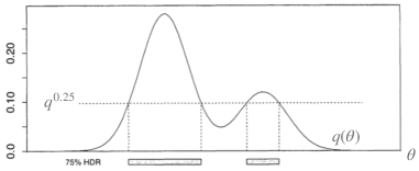
Figure 3: The $0.25$-HDR from a Normal Mixture density. This picture is a replica of [Hyndman, 1996, Figure 1]. The geometric representation of “$75\%$ probability according to $Q$” is the area between the pdf curve $q(\theta)$ and the horizontal bar corresponding to $q^{0.25}$. A higher probability coverage (according to $Q$) would correspond to a lower constant, so $q^{\alpha}<q^{0.25}$, for all $\alpha<0.25$. In the limit, we recover $100\%$ coverage at $q^{0}=0$.

Appendix D 2-Wasserstein metric

In the main portion of the paper, we endowed $\Delta_{\mathcal{X}\mathcal{Y}}$ with the $2$-Wasserstein metric. It is defined as

$$\|P-P^{\prime}\|_{W_{2}}\equiv W_{2}(P,P^{\prime}):=\sqrt{\inf_{\gamma\in\Gamma(P,P^{\prime})}\mathbb{E}_{((x_{1},y_{1}),(x_{2},y_{2}))\sim\gamma}[d((x_{1},y_{1}),(x_{2},y_{2}))^{2}]},\quad\text{where}$$

1. $P,P^{\prime}\in\Delta_{\mathcal{X}\mathcal{Y}}$;

2. $\Gamma(P,P^{\prime})$ is the set of all couplings of $P$ and $P^{\prime}$. A coupling $\gamma$ is a joint probability measure on $(\mathcal{X}\times\mathcal{Y})\times(\mathcal{X}\times\mathcal{Y})$ whose marginals are $P$ and $P^{\prime}$ on the first and second factors, respectively;

3. $d$ is the product metric endowed to $\mathcal{X}\times\mathcal{Y}$ [Deza and Deza, 2013, Section 4.2].

Appendix E Importance of Assumption 1

We need Assumption 1 in light of the results in Kessler et al. [2023]. There, the authors show that misspecified models can forget even when Bayesian inference is carried out exactly. By requiring that $\text{diam}(\mathcal{F})=r$, we control the amount of misspecification via $r$. In Kessler et al. [2023], the authors design a new approach – called Prototypical Bayesian Continual Learning, or ProtoCL – that allows dropping Assumption 1 while retaining the Bayesian benefit of remembering previous tasks. Because the main goal of this paper is to come up with a procedure that allows the designer to express preferences over the tasks, we retain Assumption 1, and we work in the classical framework of Bayesian Continual Learning. In the future, we plan to generalize our results by operating with ProtoCL.

Appendix F An example of a parametrized family $\mathcal{F}$

Let us give an example of a parametrized family $\mathcal{F}$. Suppose that we have one-dimensional data points and labels. At each task $i$, the marginal on $\mathcal{X}$ of $P_{i}$ is a Normal $\mathcal{N}(\mu,1)$, while the conditional distribution of label $y\in\mathcal{Y}$ given data point $x\in\mathcal{X}$ is a categorical $\text{Cat}(\vartheta)$. Hence, the parameter for $P_{i}$ is $\theta=(\mu,\vartheta)$, and it belongs to $\Theta=\mathbb{R}\times\mathbb{R}^{|\mathcal{Y}|}$. In this example, family $\mathcal{F}$ can be thought of as the convex hull of distributions that can be decomposed as we just described, and whose distance according to the $2$-Wasserstein metric does not exceed some $r>0$.

Appendix G Preferences induce a partial order on the tasks

Notice how $\bar{w}$ induces a preference relation $\preceq_{\bar{w}}$ on the elements of $\mathcal{T}_{k}:=\{P_{1},P_{2},\dots,P_{k}\}$, $k\geq 2$. We have that $P_{i}\preceq_{\bar{w}}P_{j}$ if and only if $w_{i}\leq w_{j}$, $i\neq j$. In other words, we favor task $j$ over task $i$ if the weight $w_{j}$ assigned to task $j$ is larger than the one assigned to task $i$. In turn, $(\mathcal{T}_{k},\preceq_{\bar{w}})$ is a poset, for all $k\geq 2$.

Appendix H Proofs of the Theorems

Proof of Theorem 1.

Without loss of generality, suppose we have encountered $i=2$ tasks so far, so the FGCS is $\mathcal{Q}^{\text{co}}_{2}$. Assume (again without loss of generality) that all the elements in posterior sets $\mathcal{Q}_{1}$ and $\mathcal{Q}_{2}$ cannot be written as a convex combination of one another. Let $\hat{Q}$ be any element in the convex hull $\mathcal{Q}^{\text{co}}_{2}$. Then, there exists a probability vector $\bar{\beta}=(\beta_{1}^{1},\ldots,\beta_{1}^{m_{1}},\beta_{2}^{1},\ldots,\beta_{2}^{m_{2}})^{\top}$ such that

$$\begin{split}\hat{Q}&=\sum_{j=1}^{m_{1}}\beta_{1}^{j}Q_{1}^{j}+\sum_{j=1}^{m_{2}}\beta_{2}^{j}Q_{2}^{j}\propto L_{1}\sum_{j=1}^{m_{1}}\beta_{1}^{j}Q_{0}^{j}+L_{1}L_{2}\sum_{j=1}^{m_{2}}\beta_{2}^{j}Q^{j}_{0}.\end{split}$$ (4)

This proportional relationship is based on the Bayesian inference (line 4) in Algorithm 1. Hence, there exists an equivalent preference $\bar{w}=(w_{1}=\sum_{j=1}^{m_{1}}\beta_{1}^{j},w_{2}=\sum_{j=1}^{m_{2}}\beta_{2}^{j})^{\top}$. ∎

Proof of Theorem 2.

For maximum generality, assume $\Theta$ is uncountable. Let $\hat{q}_{\bar{w}}$ denote the pdf of $\hat{Q}_{\bar{w}}$. The $\alpha$-level Highest Density Region $R_{\alpha}(\hat{Q}_{\bar{w}})$ is defined in Coolen [1992] as a subset of the output space such that

$$\int_{R_{\alpha}(\hat{Q}_{\bar{w}})}\hat{q}_{\bar{w}}(\theta)\text{d}\theta\geq 1-\alpha\quad\text{ and }\quad\int_{R_{\alpha}(\hat{Q}_{\bar{w}})}\text{d}\theta\text{ is a minimum.}$$

We need $\int_{R_{\alpha}(\hat{Q}_{\bar{w}})}\text{d}\theta$ to be a minimum because we want $R_{\alpha}(\hat{Q}_{\bar{w}})$ to be the smallest possible region that gives us the desired probabilistic coverage. Equivalently, from Definition 2 we know that we can write that $R_{\alpha}(\hat{Q}_{\bar{w}})=\{\theta\in\Theta:\hat{q}_{\bar{w}}(\theta)\geq\hat{q}_{\bar{w}}^{\alpha}\}$, where $\hat{q}_{\bar{w}}^{\alpha}$ is a constant value. In particular, it is the largest constant such that $\text{Pr}_{\hat{Q}_{\bar{w}}}[\theta\in R_{\alpha}(\hat{Q}_{\bar{w}})]\geq 1-\alpha$ Hyndman [1996]. Equation 3, then, comes from the fact that $\text{Pr}_{\hat{Q}_{\bar{w}}}[\theta^{\star}_{\bar{w}}\in R_{\alpha}(\hat{Q}_{\bar{w}})]=\int_{R_{\alpha}(\hat{Q}_{\bar{w}})}\hat{q}_{\bar{w}}(\theta)\text{d}\theta$, a well-known equality in probability theory Billingsley [1986]. The integral is greater than or equal to $1-\alpha$ by the definition of HDR. ∎

Appendix I Details of Experiment Setup

Our experiment code is available at an anonymous GitHub repo: https://github.com/ibcl-anon/ibcl.

I.1 Benchmarks

We select 15 tasks from CelebA. All tasks are binary image classification on celebrity face images. Each task $i$ is to classify whether the face has an attribute such as wearing eyeglasses or having a mustache. The first 15 attributes (out of 40) in the attribute list Liu et al. [2015] are selected for our tasks. The training, validation and testing sets are already split upon download, with 162,770, 19,867 and 19,962 images, respectively. All images are annotated with binary labels of the 15 attributes in our tasks. We use the same training, validation and testing set for all tasks, with labels being the only difference.

We select 20 classes from CIFAR100 Krizhevsky et al. [2009] to construct 10 Split-CIFAR100 tasks Zenke et al. [2017]. Each task is a binary image classification between an animal classes (label 0) and a non-animal class (label 1). The classes are (in order of tasks):

1. Label 0: aquarium fish, beaver, dolphin, flatfish, otter, ray, seal, shark, trout, whale.

2. Label 1: bicycle, bus, lawn mower, motorcycle, pickup truck, rocket, streetcar, tank, tractor, train.

That is, the first task is to classify between aquarium fish images and bicycle images, and so on. We want to show that the continual learning model incrementally gains knowledge of how to identify animals from non-animals throughout the task sequence. For each class, CIFAR100 has 500 training data points and 100 testing data points. We hold out 100 training data points for validation. Therefore, at each task we have 400 * 2 = 800 training data, 100 * 2 = 200 validation data and 100 * 2 = 200 testing data.

We also select 20 classes from TinyImageNet Le and Yang [2015]. The setup is similar to Split-CIFAR100, with label 0 being animals and 1 being non-animals.

1. Label 0: goldfish, European fire salamander, bullfrog, tailed frog, American alligator, boa constrictor, goose, koala, king penguin, albatross.

2. Label 1: cliff, espresso, potpie, pizza, meatloaf, banana, orange, water tower, via duct, tractor.

The dataset already splits 500, 50 and 50 images for training, validation and testing per class. Therefore, each task has 1000, 100 and 100 images for training, validation and testing, respectively.

20NewsGroups Lang [1995] contains news report texts on 20 topics. We select 10 topics for 5 binary text classification tasks. Each task is to distinguish whether the topic is computer-related (label 0) or not computer-related (label 1), as follows.

1. Label 0: comp.graphics, comp.os.ms-windows.misc, comp.sys.ibm.pc.hardware, comp.sys.mac.hardware, comp.windows.x.

2. Label 1: misc.forsale, rec.autos, rec.motorcycles, rec.sport.baseball, rec.sport.hockey.

Each class has different number of news reports. On average, a class has 565 reports for training and 376 for testing. We then hold out 100 reports from the 565 for validation. Therefore, each binary classification task has 930, 200 and 752 data points for training, validation and testing, on average respectively.

I.2 Training Configurations

All data points are first preprocessed by a feature extractor. For images, the feature extractor is a pre-trained ResNet18 He et al. [2016]. We input the images into the ResNet18 model and obtain its last hidden layer’s activations, which has a dimension of 512. For texts, the extractor is TF-IDF Aizawa [2003] succeeded with PCA to reduce the dimension to 512 as well.

Each Bayesian network model is trained with evidence lower bound (ELBO) loss, with a fixed feed-forward architecture (input=512, hidden=64, output=1). The hidden layer is ReLU-activated and the output layer is sigmoid-activated. Therefore, our parameter space $\Theta$ is the set of all values that can be taken by this network’s weights and biases.

The three variational inference priors, learning rate, batch size and number of epcohs are tuned on validation sets. The tuning results are as follows.

1. CelebA: priors = $\{\mathcal{N}(0,0.2^{2}I)$, $\mathcal{N}(0,0.25^{2}I)$, $\mathcal{N}(0,0.3^{2}I)\}$, lr = $1e-3$, batch size = $64$, epochs = $10$.

2. Split-CIFAR100: priors = $\{\mathcal{N}(0,2^{2}I)$, $\mathcal{N}(0,2.5^{2}I)$, $\mathcal{N}(0,3^{2}I)\}$, lr = $5e-4$, batch size = $32$, epochs = $50$.

3. TinyImageNet: priors = $\{\mathcal{N}(0,2^{2}I)$, $\mathcal{N}(0,2.5^{2}I)$, $\mathcal{N}(0,3^{2}I)\}$, lr = $5e-4$, batch size = $32$, epochs = $30$.

4. 20NewsGroup: priors = $\{\mathcal{N}(0,2^{2}I)$, $\mathcal{N}(0,2.5^{2}I)$, $\mathcal{N}(0,3^{2}I)\}$, lr = $5e-4$, batch size = $32$, epochs = $100$.

For the baseline methods, we use exactly the same learning rate, batch sizes and epochs. For probabilistic baseline methods (VCL and VCL-reg), we use the prior with the median standard deviation. For example, on CelebA tasks, VCL and VCL-reg uses the normal prior $\mathcal{N}(0,0.25^{2}I)$.

I.3 Evaluation Method

We use widely adopted continual learning metrics, (1) average per-task accuracy and (2) peak per-task accuracy to evaluate performance, as well as (3) backward transfer Díaz-Rodríguez et al. [2018] to evaluate resistance to catastrophic forgetting. These metrics are computed from all accuracies $acc_{ij}$ of a model at the end of task $i$ on the testing data on a previous task $j\in\{1,\dots i\}$. Specifically,

$$\begin{split}avg\_per\_task\_acc_{i}=\frac{1}{i}\sum_{l=1}^{i}acc_{ij},\,i\in\{1,\dots,N\}\\ peak\_per\_task\_acc_{i}=\max_{j\in\{1,\ldots,i\}}acc_{ij},\,i\in\{1,\dots,N\}\\ avg\_per\_task\_bt_{i}=\frac{1}{i-1}\sum_{l=2}^{i}(acc_{ij}-acc_{i(j-1)}),\,i\in\{2,\dots,N\}\end{split}$$ (5)

To obtain an $acc_{ij}$ that evaluates preference-addressing capability, at each task $i$, we randomly sample $K=10$ preferences, $\bar{w}_{i1},\dots,\bar{w}_{iK}$, over all tasks encountered so far. Therefore, GEM-reg, VCL-reg and IBCL need to generate $K$ models, one for each preference. All $K$ models are evaluated on testing data of task $j\in\{1,\dots i\}$, resulting in accuracy $acc_{ijk}$, with $k\in\{1,\dots,K\}$. We use preference as weights to compute $acc_{ij}$ as a weighted sum

$$acc_{ij}=\sum_{k=1}^{K}\frac{\bar{w}_{ik}[j]}{W_{ik}}acc_{ijk}$$ (6)

where $W_{ik}=\sum_{k=1}^{K}\bar{w}_{ik}[j]$ is the normalization factor to ensure the resulting accuracy value is in $[0,1]$. Here, $\bar{w}_{ik}[j]$ denotes the $j$-th scalar entry of preference vector $\bar{w}_{ik}$. For GEM and VCL, we only learn 1 model per task to address all preferences. To evaluate that one model’s capability in preference addressing, we use its testing accuracy in place of $acc_{ijk}$ in (6). By this computation, all accuracy scores are preference-weighted and reflect an algorithm’s ability to produce preference-addressing models.

Recall that models generated by VCL, VCL-reg and IBCL are probabilistic (BNNs for VCL and VCL-reg and HDRs for IBCL). Therefore, we sample 100 deterministic models from each of the output probabilistic models to compute $acc_{ijk}$. We record the maximum, mean and minimum values of $acc_{ijk}$ across all the sampled models. The maximum value is the estimated Pareto optimality.

Appendix J Ablation Studies

We conduct two ablation studies. The first one is on different significance level $\alpha$ in Algorithm 2.

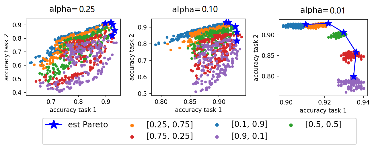
Figure 4: Different $\alpha$’s on different preferences over the first two tasks in 20NewsGroup.

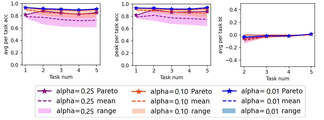
Figure 5: Different $\alpha$’s on randomly generated preferences over all tasks in 20NewsGroup.

In Figure 4, we evaluate testing accuracy on three different $\alpha$’s over five different preferences (from $[0.1,0.9]$ to $[0.9,0.1]$) on the first two tasks of 20NewsGroup. For each preference, we uniformly sample 200 deterministic models from the HDR. We use the sampled model with the maximum L2 sum of the two accuracies to estimate the Pareto optimality under a preference. We can see that, as $\alpha$ approaches 0, we tend to sample closer to the Pareto front. This is because, with a smaller $\alpha$, HDRs becomes wider and we have a higher probability to sample Pareto-optimal models according to Theorem 2. For instance, when $\alpha=0.01$, we have a probability of at least $0.99$ that the Pareto-optimal solution is contained in the HDR.

We then evaluate the three $\alpha$’s in the same way as in the main experiments, with 10 randomly generated preferences per task. Figure 5 shows that the performance drops as $\alpha$ increases, because we are more likely to sample poorly performing models from the HDR.

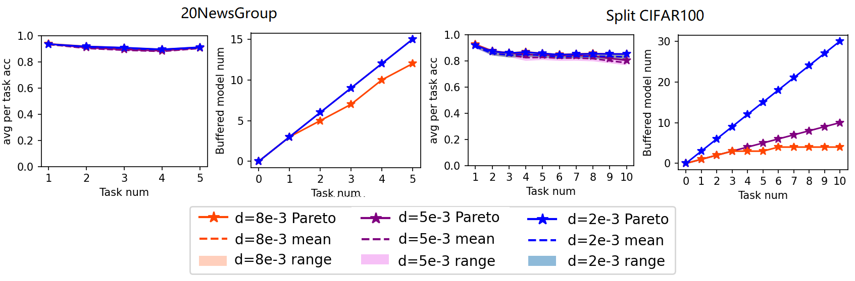
Figure 6: Different $d$’s on 20NewsGroup and Split-CIFAR100. The buffer growth curves of $d=5e-3$ and $d=2e-3$ of 20NewsGroup are overlapping.

The second ablation study is on different thresholds $d$ in Algorithm 1. As $d$ increases, we are allowing more posteriors in the knowledge base to be reused. This will lead to memory efficiency at the cost of a performance drop. Figure 6 supports this trend. We can see how performance barely drops by reusing posteriors, while the buffer growth speed becomes sublinear. For Split-CIFAR100, when $d=8e-3$, the buffer size stops growing after task 6.

References

- Abati et al. [2020] Davide Abati, Jakub Tomczak, Tijmen Blankevoort, Simone Calderara, Rita Cucchiara, and Babak Ehteshami Bejnordi. Conditional channel gated networks for task-aware continual learning. In Proceedings of the IEEE Conference on Computer Vision and Pattern Recognition, 2020.
- Aizawa [2003] Akiko Aizawa. An information-theoretic perspective of tf–idf measures. Information Processing & Management, 39(1):45–65, 2003.
- Billingsley [1986] Patrick Billingsley. Probability and Measure. John Wiley and Sons, second edition, 1986.
- Bulat et al. [2020] Adrian Bulat, Jean Kossaifi, Georgios Tzimiropoulos, and Maja Pantic. Incremental multi-domain learning with network latent tensor factorization. In Proceedings of the AAAI Conference on Artificial Intelligence. AAAI Press, 2020.
- Caprio and Gong [2023] Michele Caprio and Ruobin Gong. Dynamic imprecise probability kinematics. Proceedings of Machine Learning Research, 215:72–83, 2023.
- Caprio and Mukherjee [2023] Michele Caprio and Sayan Mukherjee. Ergodic theorems for dynamic imprecise probability kinematics. International Journal of Approximate Reasoning, 152:325–343, 2023.
- Caprio and Seidenfeld [2023] Michele Caprio and Teddy Seidenfeld. Constriction for sets of probabilities. Proceedings of Machine Learning Research, 215:84–95, 2023.
- Caprio et al. [2023] Michele Caprio, Souradeep Dutta, Kuk Jin Jang, Vivian Lin, Radoslav Ivanov, Oleg Sokolsky, and Insup Lee. Imprecise Bayesian neural networks. Available at arXiv:2302.09656, 2023.
- Caruana [1997] Rich Caruana. Multitask learning. Machine learning, 28:41–75, 1997.
- Chen and Liu [2016] Z. Chen and B. Liu. Lifelong Machine Learning. Synthesis Lectures on Artificial Intelligence and Machine Learning. Morgan & Claypool Publishers, 2016.
- Coolen [1992] Frank P. A. Coolen. Imprecise highest density regions related to intervals of measures. Memorandum COSOR, 9254, 1992.
- De Lange et al. [2021] Matthias De Lange, Rahaf Aljundi, Marc Masana, Sarah Parisot, Xu Jia, Aleš Leonardis, Gregory Slabaugh, and Tinne Tuytelaars. A continual learning survey: Defying forgetting in classification tasks. IEEE transactions on pattern analysis and machine intelligence, 44(7):3366–3385, 2021.
- Deza and Deza [2013] Michel Marie Deza and Elena Deza. Encyclopedia of Distances. Springer Berlin, Heidelberg, 2nd edition, 2013.
- Díaz-Rodríguez et al. [2018] Natalia Díaz-Rodríguez, Vincenzo Lomonaco, David Filliat, and Davide Maltoni. Don’t forget, there is more than forgetting: new metrics for continual learning. arXiv preprint arXiv:1810.13166, 2018.
- Ebrahimi et al. [2019] Sayna Ebrahimi, Mohamed Elhoseiny, Trevor Darrell, and Marcus Rohrbach. Uncertainty-guided continual learning with bayesian neural networks. arXiv preprint arXiv:1906.02425, 2019.
- Farajtabar et al. [2020] Mehrdad Farajtabar, Navid Azizan, Alex Mott, and Ang Li. Orthogonal gradient descent for continual learning. In Proceedings of the International Conference on Artificial Intelligence and Statistics, 2020.
- Farquhar and Gal [2019] Sebastian Farquhar and Yarin Gal. A unifying Bayesian view of continual learning. arXiv preprint arXiv:1902.06494, 2019.
- Finn et al. [2017] Chelsea Finn, Pieter Abbeel, and Sergey Levine. Model-Agnostic Meta-Learning for fast adaptation of deep networks. In Doina Precup and Yee Whye Teh, editors, Proceedings of the 34th International Conference on Machine Learning, volume 70 of Proceedings of Machine Learning Research, pages 1126–1135. PMLR, 2017.
- Gupta et al. [2021] Soumyajit Gupta, Gurpreet Singh, Raghu Bollapragada, and Matthew Lease. Scalable unidirectional pareto optimality for multi-task learning with constraints. arXiv preprint arXiv:2110.15442, 2021.
- He et al. [2016] Kaiming He, Xiangyu Zhang, Shaoqing Ren, and Jian Sun. Deep residual learning for image recognition. In Proceedings of the IEEE conference on computer vision and pattern recognition, pages 770–778, 2016.
- He et al. [2018] Xiaoxi He, Zimu Zhou, and Lothar Thiele. Multi-task zipping via layer-wise neuron sharing. Advances in Neural Information Processing Systems, pages 6016–6026, 2018.
- Hyndman [1996] Rob J. Hyndman. Computing and graphing highest density regions. The American Statistician, 50(2):120–126, 1996.
- Juat et al. [2022] Ngumbang Juat, Mike Meredith, and John Kruschke. Package ‘hdinterval’, 2022. URL https://cran.r-project.org/web/packages/HDInterval/HDInterval.pdf. Accessed on May 9, 2023.
- Kao et al. [2021] Ta-Chu Kao, Kristopher Jensen, Gido van de Ven, Alberto Bernacchia, and Guillaume Hennequin. Natural continual learning: success is a journey, not (just) a destination. Advances in Neural Information Processing Systems, 34:28067–28079, 2021.
- Kendall et al. [2018] Alex Kendall, Yarin Gal, and Roberto Cipolla. Multi-task learning using uncertainty to weigh losses for scene geometry and semantics. In Proceedings of the IEEE conference on computer vision and pattern recognition, pages 7482–7491, 2018.
- Kessler et al. [2023] Samuel Kessler, Adam Cobb, Tim G. J. Rudner, Stefan Zohren, and Stephen J. Roberts. On sequential bayesian inference for continual learning. arXiv preprint arXiv:2301.01828, 2023.
- Kim et al. [2023] Sanghwan Kim, Lorenzo Noci, Antonio Orvieto, and Thomas Hofmann. Achieving a better stability-plasticity trade-off via auxiliary networks in continual learning. arXiv preprint arXiv:2303.09483, 2023.
- Kirkpatrick et al. [2017a] James Kirkpatrick, Razvan Pascanu, Neil Rabinowitz, Joel Veness, Guillaume Desjardins, Andrei A. Rusu, Kieran Milan, John Quan, Tiago Ramalho, Agnieszka Grabska-Barwinska, Demis Hassabis, Claudia Clopath, Dharshan Kumaran, and Raia Hadsell. Overcoming catastrophic forgetting in neural networks. Proceedings of the National Academy of Sciences, 114(13):3521–3526, 2017a.
- Kirkpatrick et al. [2017b] James Kirkpatrick, Razvan Pascanu, Neil Rabinowitz, Joel Veness, Guillaume Desjardins, Andrei A Rusu, Kieran Milan, John Quan, Tiago Ramalho, Agnieszka Grabska-Barwinska, et al. Overcoming catastrophic forgetting in neural networks. Proceedings of the national academy of sciences, 114(13):3521–3526, 2017b.
- Krizhevsky et al. [2009] Alex Krizhevsky, Geoffrey Hinton, et al. Learning multiple layers of features from tiny images. 2009.
- Lang [1995] Ken Lang. Newsweeder: Learning to filter netnews. In Machine learning proceedings 1995, pages 331–339. Elsevier, 1995.
- Le and Yang [2015] Ya Le and Xuan Yang. Tiny imagenet visual recognition challenge. CS 231N, 7(7):3, 2015.
- Lee et al. [2017] Sang-Woo Lee, Jin-Hwa Kim, Jaehyun Jun, Jung-Woo Ha, and Byoung-Tak Zhang. Overcoming catastrophic forgetting by incremental moment matching. Advances in neural information processing systems, 30, 2017.
- Lee et al. [2019] Seungwon Lee, James Stokes, and Eric Eaton. Learning shared knowledge for deep lifelong learning using deconvolutional networks. In IJCAI, pages 2837–2844, 2019.
- Li et al. [2020] Honglin Li, Payam Barnaghi, Shirin Enshaeifar, and Frieder Ganz. Continual learning using bayesian neural networks. IEEE transactions on neural networks and learning systems, 32(9):4243–4252, 2020.
- Lin et al. [2019] Xi Lin, Hui-Ling Zhen, Zhenhua Li, Qing-Fu Zhang, and Sam Kwong. Pareto multi-task learning. Advances in neural information processing systems, 32, 2019.
- Lin et al. [2020] Xi Lin, Zhiyuan Yang, Qingfu Zhang, and Sam Kwong. Controllable pareto multi-task learning. arXiv preprint arXiv:2010.06313, 2020.
- Liu et al. [2015] Ziwei Liu, Ping Luo, Xiaogang Wang, and Xiaoou Tang. Deep learning face attributes in the wild. In Proceedings of International Conference on Computer Vision (ICCV), December 2015.
- Lopez-Paz and Ranzato [2017] David Lopez-Paz and Marc’Aurelio Ranzato. Gradient episodic memory for continual learning. Advances in neural information processing systems, 30, 2017.
- Lu et al. [2017] Yongxi Lu, Abhishek Kumar, Shuangfei Zhai, Yu Cheng, Tara Javidi, and Rogério Feris. Fully-adaptive feature sharing in multi-task networks with applications in person attribute classification. In Proceedings of the IEEE Conference on Computer Vision and Pattern Recognition, 2017.
- Ma et al. [2020] Pingchuan Ma, Tao Du, and Wojciech Matusik. Efficient continuous pareto exploration in multi-task learning. In International Conference on Machine Learning, pages 6522–6531. PMLR, 2020.
- Mahapatra and Rajan [2020] Debabrata Mahapatra and Vaibhav Rajan. Multi-task learning with user preferences: Gradient descent with controlled ascent in pareto optimization. In International Conference on Machine Learning, pages 6597–6607. PMLR, 2020.
- Mendez and Eaton [2021] Jorge A. Mendez and Eric Eaton. Lifelong learning of compositional structures. In Proceedings of the International Conference on Learning Representations, 2021.
- Navon et al. [2020] Aviv Navon, Aviv Shamsian, Gal Chechik, and Ethan Fetaya. Learning the pareto front with hypernetworks. arXiv preprint arXiv:2010.04104, 2020.
- Nguyen et al. [2018] Cuong V. Nguyen, Yingzhen Li, Thang D. Bui, and Richard E. Turner. Variational continual learning. In International Conference on Learning Representations, 2018. URL https://openreview.net/forum?id=BkQqq0gRb.
- Parisi et al. [2019] German I Parisi, Ronald Kemker, Jose L Part, Christopher Kanan, and Stefan Wermter. Continual lifelong learning with neural networks: A review. Neural networks, 113:54–71, 2019.
- Raghavan and Balaprakash [2021] Krishnan Raghavan and Prasanna Balaprakash. Formalizing the generalization-forgetting trade-off in continual learning. Advances in Neural Information Processing Systems, 34:17284–17297, 2021.
- Ramesh and Chaudhari [2022] Rahul Ramesh and Pratik Chaudhari. Model zoo: A growing brain that learns continually. In Proceedings of the International Conference on Learning Representations, 2022. URL https://openreview.net/forum?id=WfvgGBcgbE7.
- Riemer et al. [2019] Matthew Riemer, Ignacio Cases, Robert Ajemian, Miao Liu, Irina Rish, Yuhai Tu, and Gerald Tesauro. Learning to learn without forgetting by maximizing transfer and minimizing interference. In Proceedings of the International Conference on Learning Representations, 2019.
- Robins [1995] Anthony Robins. Catastrophic forgetting, rehearsal and pseudorehearsal. Connection Science, 7(2):123–146, 1995.
- Rolnick et al. [2019] David Rolnick, Arun Ahuja, Jonathan Schwarz, Timothy Lillicrap, and Gregory Wayne. Experience replay for continual learning. In H. Wallach, H. Larochelle, A. Beygelzimer, F. d'Alché-Buc, E. Fox, and R. Garnett, editors, Advances in Neural Information Processing Systems, volume 32. Curran Associates, Inc., 2019. URL https://proceedings.neurips.cc/paper_files/paper/2019/file/fa7cdfad1a5aaf8370ebeda47a1ff1c3-Paper.pdf.
- Rusu et al. [2016] Andrei A. Rusu, Neil C. Rabinowitz, Guillaume Desjardins, Hubert Soyer, James Kirkpatrick, Koray Kavukcuoglu, Razvan Pascanu, and Raia Hadsell. Progressive neural networks. arXiv preprint arXiv:1606.04671, 2016.
- Ruvolo and Eaton [2013a] P. Ruvolo and E. Eaton. Active task selection for lifelong machine learning. Proceedings of the AAAI Conference on Artificial Intelligence, 27(1), 2013a.
- Ruvolo and Eaton [2013b] Paul Ruvolo and Eric Eaton. ELLA: An efficient lifelong learning algorithm. In Sanjoy Dasgupta and David McAllester, editors, Proceedings of the 30th International Conference on Machine Learning, volume 28 of Proceedings of Machine Learning Research, pages 507–515. PMLR, 17–19 Jun 2013b. URL https://proceedings.mlr.press/v28/ruvolo13.html.
- Schwarz et al. [2018] Jonathan Schwarz, Wojciech Czarnecki, Jelena Luketina, Agnieszka Grabska-Barwinska, Yee Whye Teh, Razvan Pascanu, and Raia Hadsell. Progress & compress: A scalable framework for continual learning. In International Conference on Machine Learning, pages 4528–4537. PMLR, 2018.
- Sener and Koltun [2018] Ozan Sener and Vladlen Koltun. Multi-task learning as multi-objective optimization. Advances in neural information processing systems, 31, 2018.
- Serra et al. [2018] Joan Serra, Didac Suris, Marius Miron, and Alexandros Karatzoglou. Overcoming catastrophic forgetting with hard attention to the task. In Proceedings of the International Conference on Machine Learning, pages 4548–4557, 2018.
- Servia-Rodriguez et al. [2021] Sandra Servia-Rodriguez, Cecilia Mascolo, and Young D Kwon. Knowing when we do not know: Bayesian continual learning for sensing-based analysis tasks. arXiv preprint arXiv:2106.05872, 2021.
- Silver et al. [2013] D. L. Silver, Q. Yang, and L. Li. Lifelong machine learning systems: Beyond learning algorithms. In 2013 AAAI spring symposium series, 2013.
- Suteu and Guo [2019] Mihai Suteu and Yike Guo. Regularizing deep multi-task networks using orthogonal gradients. CoRR, abs/1912.06844, 2019.
- Tang et al. [2021] Shixiang Tang, Peng Su, Dapeng Chen, and Wanli Ouyang. Gradient regularized contrastive learning for continual domain adaptation. Proceedings of the AAAI Conference on Artificial Intelligence, 35(3):2665–2673, May 2021. doi: 10.1609/aaai.v35i3.16370. URL https://ojs.aaai.org/index.php/AAAI/article/view/16370.
- Thrun [1998] Sebastian Thrun. Lifelong learning algorithms. Learning to learn, 8:181–209, 1998.
- Troffaes and de Cooman [2014] Matthias C. M. Troffaes and Gert de Cooman. Lower Previsions. Wiley Series in Probability and Statistics. New York : Wiley, 2014.
- Vandenhende et al. [2019] Simon Vandenhende, Bert De Brabandere, and Luc Van Gool. Branched multi-task networks: deciding what layers to share. CoRR, abs/1904.02920, 2019.
- Von Oswald et al. [2019] Johannes Von Oswald, Christian Henning, Benjamin F Grewe, and João Sacramento. Continual learning with hypernetworks. arXiv preprint arXiv:1906.00695, 2019.
- Walley [1991] Peter Walley. Statistical Reasoning with Imprecise Probabilities, volume 42 of Monographs on Statistics and Applied Probability. London : Chapman and Hall, 1991.
- Xu et al. [2021] Ju Xu, Jin Ma, Xuesong Gao, and Zhanxing Zhu. Adaptive progressive continual learning. IEEE transactions on pattern analysis and machine intelligence, PP, 07 2021. doi: 10.1109/TPAMI.2021.3095064.
- Yang and Hospedales [2017] Yongxin Yang and Timothy Hospedales. Deep multi-task representation learning: a tensor factorisation approach. In Proceedings of the International Conference on Learning Representations, 2017.
- Yoon et al. [2018a] Jaehong Yoon, Eunho Yang, and Sungju Hwang. Lifelong learning with dynamically expandable networks. In Proceedings of the International Conference on Learning Representations, 2018a.
- Yoon et al. [2020] Jaehong Yoon, Saehoon Kim, Eunho Yang, and Sungju Hwang. Scalable and order-robust continual learning with additive parameter decomposition. In Proceedings of the International Conference on Learning Representations, 2020.
- Yoon et al. [2018b] Jaesik Yoon, Taesup Kim, Ousmane Dia, Sungwoong Kim, Yoshua Bengio, and Sungjin Ahn. Bayesian Model-Agnostic Meta-Learning. In S. Bengio, H. Wallach, H. Larochelle, K. Grauman, N. Cesa-Bianchi, and R. Garnett, editors, Advances in Neural Information Processing Systems, volume 31. Curran Associates, Inc., 2018b.
- Zenke et al. [2017] Friedemann Zenke, Ben Poole, and Surya Ganguli. Continual learning through synaptic intelligence. In International conference on machine learning, pages 3987–3995. PMLR, 2017.