Phases of ⁴He and H₂ adsorbed on a single carbon nanotube

Abstract

Using a diffusion Monte Carlo (DMC) technique, we calculated the phase diagrams of ⁴He and H₂ adsorbed on a single (5,5) carbon nanotube, one of the narrowest that can be obtained experimentally. For a single monolayer, when the adsorbate density increases, both species undergo a series of first order solid-solid phase transitions between incommensurate arrangements. Remarkably, the ⁴He lowest-density solid phase shows supersolid behavior in contrast with the normal solid that we found for H₂. The nature of the second-layer is also different for both adsorbates. Contrarily to what happens on graphite, the second-layer of ⁴He on that tube is a liquid, at least up to the density corresponding to a third-layer promotion on a flat substrate. However, the second-layer of H₂ is a solid that, at its lowest stable density, has a small but observable superfluid fraction.

I Introduction

A carbon nanotube can be thought of as the result of folding a single graphene sheet over itself to form a seamless cylinder [1]. It is then a quasi-one dimensional (1D) structure that can be coated with different kinds of adsorbates. In principle, that reduced dimensionality could produce phase diagrams different than those on quasi-two dimensional (2D) environments such as graphite or graphene. The study of the adsorption capabilities of those carbon cylinders is possible since an isolated carbon nanotube can be synthesized and made to work as a mechanical resonator. Its resonant frequencies change upon loading, allowing in this way an accurate determination of the adsorbate phases [2, 3, 4, 5, 6, 7, 8]. In principle, this resonant frequency can be monitored to check if we have a supersolid structure, as it was done for the second layer of ⁴He on graphite [9, 10].

Experimental studies on Ne, Ar, and Kr [2, 3, 6] indicate that the first layers of those gases on nanotubes are qualitatively similar to those found in their flat equivalents, the only difference being the smaller binding energies on the cylinders due to their curved nature [2, 3]. On the other hand, it is known that ⁴He on a single nanotube is adsorbed on a layer-by-layer process, similar to the deposition on graphite [7]. The main goal of our present work is to deeply study the behavior of ⁴He and H₂ on top of a (5,5) carbon nanotube, both the first and second layers. We chose that tube since its narrowness, with a radius of $3.42$ Å, makes any difference with a flat graphite (or graphene) substrate larger than for thicker tubes. In particular, we were interested to study if the imposed curvature produced any additional phase, such as the supersolids experimentally detected [9, 11, 10] and theoretically predicted in the first [12] and second layer of ⁴He on a carbon substrate [13], or in the second layer of H₂ on graphite [14]. That superfluidity, in the first layer solids, was not calculated in previous studies [15, 16]. We also explored the possibility of second-layer liquid phases for both species.

The rest of the paper is organized as follows. The diffusion Monte Carlo method used in our study is discussed in Sec. II. Sec. III comprises the results obtained, with special attention to the stable phases of both ⁴He and H₂ adsorbed on the nanotube. The results for the superfluid fraction were calculated by the standard winding number estimator, in the limit of zero temperature. Finally, the main conclusions and discussion of the results are contained in Sec. IV.

II Method

To study the stability of the different phases, we calculated the respective ground states ($T=0$) of ⁴He atoms/H₂ molecules on a corrugated carbon nanotube at several densities. This means to write down and solve the many-body Schrödinger equation that describes the adsorbate. Following previous works in similar systems, the Hamiltonian could be written down as

$$H=\sum_{i=1}^{N}\left[-\frac{\hbar^{2}}{2m}\nabla_{i}^{2}+V_{{\rm ext}}(x_{i},y_{i},z_{i})\right]+\sum_{i<j}^{N}V_{{\rm pair}}(r_{ij})\ ,$$ (1)

where $x_{i}$, $y_{i}$, and $z_{i}$ are the coordinates of the each of the $N$ adsorbate particles with mass $m$. $V_{{\rm ext}}(x_{i},y_{i},z_{i})$ is the interaction potential between each atom or molecule and all the individual carbon atoms in the nanotube, that is considered to be a rigid structure. Those potentials are of Lennard-Jones type, with standard parameters taken from Ref. 17 in the case of ⁴He-C, and from Ref. [18] for the H₂-C interaction. $V_{\rm{pair}}$ accounts for the ⁴He-⁴He and H₂-H₂ interactions (Aziz [19] and Silvera and Goldman [20] potentials, respectively), that depend only on the distance $r_{ij}$ between particles $i$ and $j$. Both potentials are the standard models in previous literature.

To actually solve the many-body Schrödinger equation derived from the Hamiltonian in Eq. 1, we resorted to the diffusion Monte Carlo (DMC) algorithm. This stochastic numerical technique obtains, within some statistical noise, relevant ground-state properties of the $N$-particle system. To guide the diffusion process involved in DMC, one introduces a trial wave function which acts as importance sampling, reducing the variance to a manageable level. The trial wave functions used in our work derive from similar forms used previously in DMC calculations of ⁴He and H₂ on graphene and graphite [21, 22, 13, 14], that were able to reproduce available experimental data [23, 24, 25, 26, 9, 10, 27]. We are then confident that the trial wave functions used in the present work will also provide a reasonable description of the adsorbates on a similar, albeit curved, substrate.

In the present case, the trial wave function was built as a product of two terms. The first one is of Jastrow type between the adsorbate particles,

$$\Phi_{J}({\bf r}_{1},\ldots,{\bf r}_{N})=\prod_{i<j}^{N}\exp\left[-\frac{1}{2}\left(\frac{b}{r_{ij}}\right)^{5}\right]\,$$ (2)

with $b$ a variationally optimized parameter, whose values were $3.07$ Å for the ⁴He-⁴He case [15] and $3.195$ Å for the H₂-H₂ pair [16]. The second part incorporates the presence of the C atoms and localization terms,

$$\Phi_{s}({\bf r}_{1},\ldots,{\bf r}_{N})=\prod_{i}^{N}\prod_{J}^{N_{C}}\exp\left[-\frac{1}{2}\left(\frac{b_{{\text{C}}}}{r_{iJ}}\right)^{5}\right]$$

$$\times\prod_{I=1}^{N}\left[\sum_{i=1}^{N}\exp\{-c_{1,2}[({\bf r}_{i}-{\bf r}_{\text{site},I})^{2}]\}\ \right]\times\prod_{i}^{N}\Psi(R_{i}).\ \ \ \ \ \$$ (3)

Here, $N_{C}$ stands for the number of carbon atoms of the nanotube while the parameters $b_{C}$ were taken from previous calculations on the same substrates [15, 16]. $r_{iJ}$ are the distances between a particle $i$ (⁴He or H₂), and a carbon atom, $J$. $\Psi(R_{i})$ is a one-body function that depends on the radial distance of those particles to the central axis of the tube, $R_{i}$. For an atom or molecule located on the layer closest to the carbon substrate, those were taken from Refs. 15 and 16 for ⁴He and H₂. Those functions have maxima located at distances from the center of 6.26 and 6.36 Å, respectively. On the other hand, and following the procedure already used for graphite [13, 14, 28], we radially confined particles in the second layer by Gaussian functions, with variationally-optimized parameters.

The remaining part of Eq. 3 allows us to distinguish between a translationally invariant liquid ($c_{1,2}$= 0) and a (super)solid phase ($c_{1,2}\neq$ 0). Labels 1 and 2 stand for first and second layers, respectively. For solids, the values of $c_{1,2}$ were variationally optimized to obtain the minimum energies for each species and density. For particles in the first layer, the parameters for the solid where found to be identical to those obtained for flat graphene and used in previous calculations for similar systems [15, 16]. This means we used linear extrapolations between $c_{1}$ = 0.15Å^-2 (for a density of 0.08 Å^-2) and $c_{1}$ = 0.77Å^-2 (for 0.1 Å^-2) for ⁴He [21] and between $c_{1}$ = 0.61Å^-2 (for 0.08 Å^-2) and $c_{1}$ = 1.38Å^-2 (for 0.1 Å^-2) in the case of H₂ [22]. For lower densities we used the value corresponding to 0.08Å^-2 and for larger ones, the one corresponding to 0.1 Å^-2. For the second layer of H₂, $c_{2}$ = 0.46 Å^-2 was used for all densities. The optimal $c_{2}$ parameter ⁴He was $c_{2}$=0, that corresponds to a liquid (see below). For any value of $c_{1,2}$, the form of the trial function allows the ⁴He atoms and the H₂ molecules to be involved in exchanges and recover indistinguishability, a necessary ingredient to model a supersolid [12]. Alternatively, for solid phases one can use a simplified version of Eq. 3 in which each particle is pinned to a single crystallographic site. This is the ansatz used to describe first-layer phases in Refs. [15, 16] and would produce, by construction, normal solids. When we used that approximation, we obtained higher or equal energies per particle than when we use Eq. 3. The case of the equal values for the energies correspond to cases in which the superfluid estimator is equal to zero, i.e., when we recover the normal behavior of the solid.

Finally, in Eq. 3, $x_{\text{site}},y_{\text{site}}$, and $z_{\text{site}}$ are the crystallographic positions that define the solids we wrap around the (5,5) tube. Those are incommensurate arrangements built up by locating a given number, $n$, of adsorbate particles on planes perpendicular to the main axis of the nanotube. One can visualize those phases by imagining that the coated cylinder is fully cut longitudinally to have a long rectangle in which the shorter side corresponds to the length of the circumference that defines the tube. In the case of a first ⁴He layer, this means 2$\pi\times$ 6.26 Å(see above). On that short side, we locate $n$ atoms or molecules uniformly spaced, with a distance between them in the transverse (short) direction of $d_{t}$Å, and added as many parallel rows as the length of the tube will allow. Those arrays of atoms will be separated by a longitudinal distance of $d_{l}$ Å. Between those rows, we will include another one separated $d_{l}$/2 from the contiguous lines, and whose particles will be displaced $d_{t}$/2 in transverse direction with respect to the previous and following lines. A similar procedure is used to build the solids in the second layer, located at an averaged distances for the center or the tube of 8.98 and 9.42 Å for ⁴He and H₂, respectively. Since we started by $n$ particles located on rows in the transverse direction, following Refs. 16 and 15, we name these phases $n$-in-a-row solids. A picture of one of those phases can be found in Ref. 16 for the case of H₂.

The data presented in this paper are the mean of ten independent DMC simulations, and the error bars, when shown, correspond to the variance of these calculations. Every DMC history consists of 1.2$\times$10⁵ steps involving a movement of all the particles of each of the 300 replicas (walkers) that describe the different configurations. Larger number of walkers or longer simulations do not change the averages given. The values of the observables presented here were calculated after equilibration (2$\times$10⁴ time steps), i.e., when no obvious drift in their values as a function of the simulation time was detected. We made the simulations on isolated tubes, what means that periodic boundary conditions were applied only on the direction corresponding to the length of the tube. The number of particles in the simulation cells and their lengths were varied to produce the desired densities for any of the two adsorbates. The first number was between a minimum of 100 (for a one-layered tube) to a maximum of 364 for the highest densities considered in this work. However, some simulations including up to 500 particles were made to verify that our results were not affected by size effects. Conversely, the lengths of the simulation cells varied in the range 33-45 Å.

III Results

III.1 ⁴He

We first study the phase diagram of ⁴He on a (5,5) nanotube, including the promotion from a first to a second layer. Fig. 1 gives us the energy per particle for the different first-layer incommensurate solids. Those extend the results given in Ref. 15 in a double way. First, we consider now larger Helium densities in the 7-in-a-row solid, what would allow us to study all the possible first-order transitions between incommensurate arrangements up to the second-layer promotion. In addition, since those first-layer solids are described by Eq. 3, instead of having each particle of the solid pinned to a single crystallographic position (Nosanow-Jastrow wave function), we can access to any possible supersolid phases.

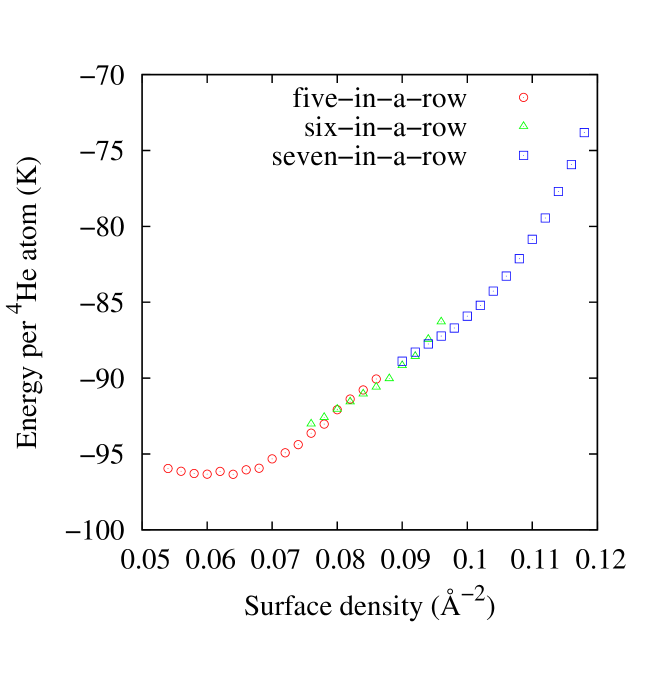
Figure 1: Energy per ⁴He atom as a function of the density, for $n$-in-a-row ($n=5,6,7$) first layer solids.

The energy per particle for any of the three $n$-in-a-row ⁴He ($n=5,6,7$) solids are shown in Fig. 1. As indicated above, to calculate the surface densities we used cylinders with a radius given by the average distance of the ⁴He atoms to the center of the tube, in this case $6.26$ Å. We do not show in Fig. 1 the results of a translationally invariant liquid phase because the energies for that phase are above the ones shown in that figure. The same applies to the $2/5$, $3/7$, and $\sqrt{3}\times\sqrt{3}$ registered solids [26]. By means of a least-squares fit method to the 5-in-a-row data, we can obtain the minimum density and its corresponding energy per particle. The results are given in Table 1. There, we can see that they are slightly different from those of Ref. 15, with $\rho=0.062$ Å^-2 and $E=-96.10$ K The reason for the discrepancy is the 5-in-a-row solid being a supersolid instead of the normal solid previously considered. Its superfluid density was calculated using the zero-temperature winding number estimator, derived in Ref. 29,

$$\frac{\rho_{s}}{\rho}=\lim_{\tau\to\infty}\alpha\left(\frac{D_{s}(\tau)}{\tau}\right)\ ,$$ (4)

with $\tau$ the imaginary time used in the quantum Monte Carlo simulation. Here, $\alpha=N/(2D_{0})$, with $D_{0}=\hbar^{2}/(2m)$, and $D_{s}(\tau)=\langle[{\bf R}_{CM}(\tau)-{\bf R}_{CM}(0)]^{2}\rangle$. ${\bf R}_{CM}$ is the position of the center of mass of the $N$ ⁴He atoms in the simulation box, using only their $z$ coordinates on which periodic boundary conditions are applied.

Table 1: Lowest and highest stability density limits for the different single-layer solid phases adsorbed on a (5,5) carbon nanotube. We include also the lowest stable density limit for the second layer of ⁴He, a liquid, and of H₂, a solid. The error bars are given in parenthesis and correspond to the last decimal place given.

$\rho$ (4He) (Å-2)	E (4He) (K)	$\rho$ (H2) (Å-2)	E (H2) (K)
5-in-a row
0.0605(5)	-96.5(1)	0.062(2)	-349.0(1)
0.076(1)	-93.7(1)	0.068(2)	-346.1(1)
6-in-a-row
0.086(2)	-90.6(1)	0.080(2)	-334.1(1)
0.088(1)	-90.0(1)	0.085(2)	-326.7(1)
7-in-a-row
0.096(2)	-87.2(1)	0.0925(5)	-314.3(1)
0.110(2)	-80.9(1)	0.0975(5)	-304.1(1)
second layer
0.181(1)	-48.9(1)	0.166(2)	-199.7(1)

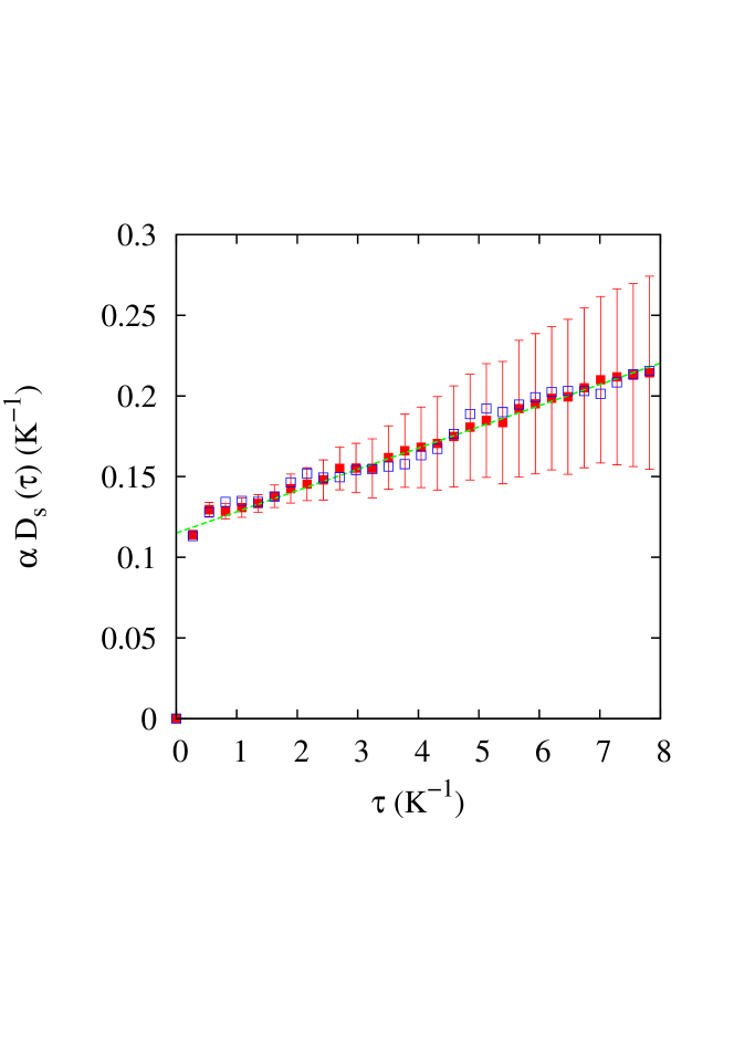
Figure 2: Estimator of the superfluid density for the first-layer 5-in-a-row supersolid ⁴He phase at $\rho$ = 0.062 Å^-2 (solid squares) and $\rho$ = 0.062 Å^-2 (open squares). The straight line is a linear least-squares fit to the $\rho$ = 0.062 Å^-2 data for $\tau>$ 3 K^-1.

The results of the superfluid estimator to the 5-in-a-row solid can be seen in Fig 2 for $\rho=0.062$ Å^-2 (solid squares) and 0.064 Å^-2 (open squares). The line is a least-square fitting to $\alpha D_{s}(\tau)$ versus $\tau$ for the lowest density in the range 3 $<\tau<$ 8 K^-1. The value obtained is $\rho_{s}/\rho$ = 1.31$\pm$0.05 % for 0.062 Å^-2 and $\rho_{s}/\rho$ = 1.35$\pm$0.05 % (line not shown) for 0.064 Å^-2. In both cases, the superfluid fraction is of the same order, but slightly larger, that the one found for a registered phase of $\rho$ = 0.0636 Å^-2 of ⁴He on graphene ($\rho_{s}/\rho$ = 0.67$\pm$0.01 %) [12]. No significant size effects were found for larger simulation cells, in accordance with results in Ref. 14.

Using the data reported in Fig. 1, and by means of double-tangent Maxwell constructions, we can obtain the stability limits of the different first-layer ⁴He solid phases. The results are given in Table 1, where we can find the lowest and highest stable densities, $\rho$, for those arrangements. This means that, for instance, there is a first-order phase transition between a 5-in-a-row solid of $\rho$ = 0.076 Å^-2 and a 6-in-a-row one with $\rho$ = 0.086 Å^-2 and the same can be said for a 6-in-a-row of $\rho$ = 0.088 Å^-2 and 7-in-a-row $\rho$ = 0.096 Å^-2 structures. Both 6- and 7-in a row solids are normal solids, with $\rho_{s}/\rho$ = 0.

If we keep increasing the ⁴He density on top of the nanotube, it is promoted to a second layer. To obtain the stability range of that second layer, we used the same technique as in Ref. 30, i.e., we calculated the energies per particle for arrangements in which the first layers were 7-in-a-row solids with different densities and put on top an increasing number of ⁴He atoms. Then, the stable second-layer will be the one with the lowest energy for a given total density. That density is calculated as the sum of the first-layer one, in which we used as an adsorbent surface a cylinder or radius 6.26 Å, and the one corresponding to the second layer, computed using another cylinder whose distance from the axis of the tube was 8.98 Å. Both radii corresponds to the mean distances of the atoms to the center of the tubes.

The results of the calculations for different ⁴He loadings are displayed in Fig. 3. In that figure, we can see that the lowest two-layer structure has a 7-in-a-row first layer solid underneath with $\rho$= 0.110 Å^-2 (full circles) for low densities, and changes to a similar structure with $\rho$= 0.115 Å^-2 upon loading (full squares). In the $x$-axis we show the inverse of the density, or surface area, since in that way we can show the double-tangent Maxwell construction between a single layer solid and the liquid on top of it. That construction, shown in Fig. 3 as a dotted line, indicates that the coexistence region is between total densities of 0.110 Å^-2 and 0.181 Å^-2 (see Table 1). For that last structure, the density of the solid close to the nanotube is $\rho$= 0.115 Å^-2. This means that, as in the case of the ⁴He adsorption on graphite, there is a compression of the layer close to the carbon when a second adsorbate sheet is deposited on top of it [30].

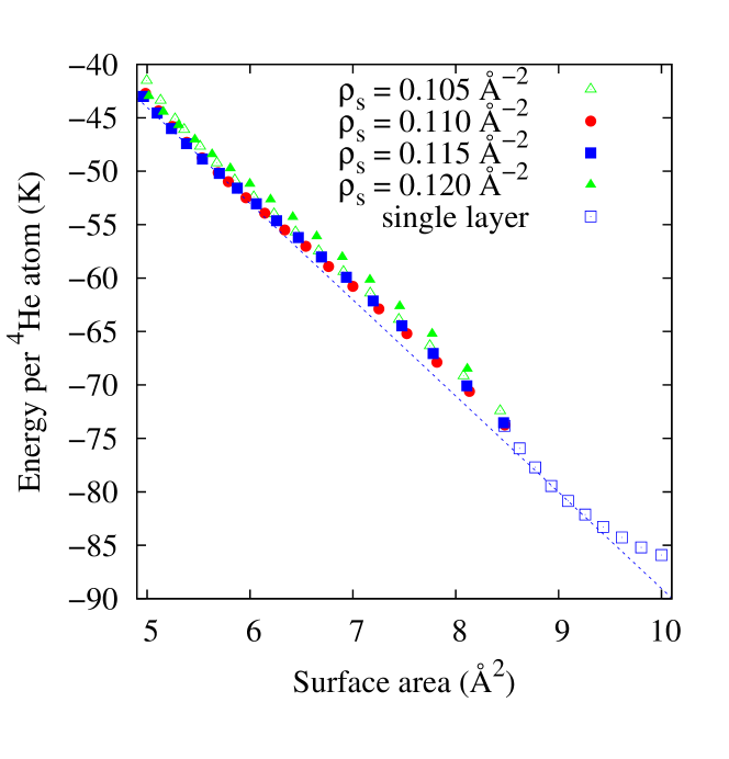
Figure 3: Energy per ⁴He atoms as a function of the inverse of the total ⁴He density in the range in which we can have first-only and first and second adsorbate layers. Full squares, 7-in-a row solids of different densities. Solid symbols, two-layer structures with different values of the densities 7-in-a-row solids (shown) underneath. In all cases, the second layers were translationally invariant liquid structures. The dotted line is a Maxwell construction between the stable densities of first-only and first+second layers. The error bars are of the size of the symbols and not shown for simplicity.

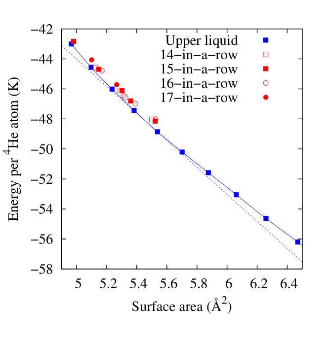
Figure 4: Same as in Fig. 3, but for surface areas in the range 5-6.5 Ų. The dotted line is also the same Maxwell construction between the stable densities of first-only and first+second layers. The full line is a guide-to-the-eye to the results of a structure in which the second layer is a liquid. We also show simulation results for different unstable $n$-in-a-row second layer-solids. The error bars are of the size of the symbols.

To see more clearly the lowest stability limit of the two-layer structure, we display in Fig. 4 a blown-up version of Fig. 3 for total surface areas in the range 5-6.5 Ų. The first value corresponds to the inverse of the experimental density for the promotion to a third layer of ⁴He on graphite [9]. It displays the same Maxwell construction line as in the previous figure as a dotted line. We included also the results for several $n$-in-a row solid structures, with $n$ in the range 14-17. Those data were obtained fixing the $c_{2}$ parameter in Eq. 3 to 0.30 Å^-2, but they are qualitatively similar to any simulation results in which $c_{2}\neq$ 0, i.e., arrangements with two solid layers are always metastable with respect to other with a liquid surface on top. In this, the behavior of ⁴He is different than of its flat counterpart adsorbed on graphite, that solidifies before a third-layer promotion [25, 26, 23, 24]. Obviously, that second-layer liquid is a superfluid, since the value of $\rho_{s}/\rho$ obtained applying Eq. 4 is 1.

III.2 H₂

We will turn now our attention to H₂, dealing first with first-layer solids described by Eq. 3 that does not pin the H₂ molecules to a single crystallographic position, as it was done in Ref. 16. This open the possibility of having supersolids, possibility that, as we will see below, is not fulfilled.

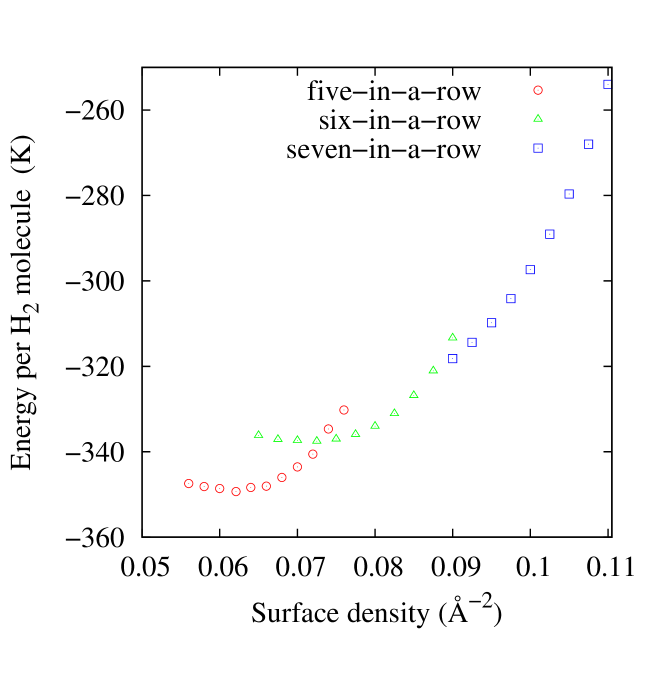
Figure 5: Same as in Fig. 1 for first-layer H₂ solids.

Fig. 5 is the H₂ counterpart of the Fig. 1 for ⁴He. The densities in the $x$-axis are calculated now using adsorbate cylinders of radius 6.36 Å. This difference is due to the larger size of the H₂ molecule with respect to the ⁴He atom. Making use of the double tangent Maxwell construction lines between those solids, we find a range of densities, shown in Table 1, for which we have stable 5-in-a-row and 6-in-a-row solids. In this case, and contrarily to what happens to ⁴He, both the stability limits and the energies per particle are basically identical to those found in Ref. 16. The reason can be understood by looking at Fig. 6. There, we can see (open symbols) the same estimator for the superfluid density shown in Fig. 2 but for a first-layer H₂ solid at $\rho$ = 0.062 Å^-2, the minimum of the 5-in-a-row energy curve in Fig. 5. We can see that $\alpha$ D${}_{s}(\tau)$ versus $\tau$ is constant for large $\tau$, indicating a zero superfluid density. This means we have a first-layer normal solid as in Ref. 16. The differences between Figs. 1 and 5 can be ascribed basically to the nature of the interparticle interactions: the larger the potential well, the more clearly are the limits between the phases.

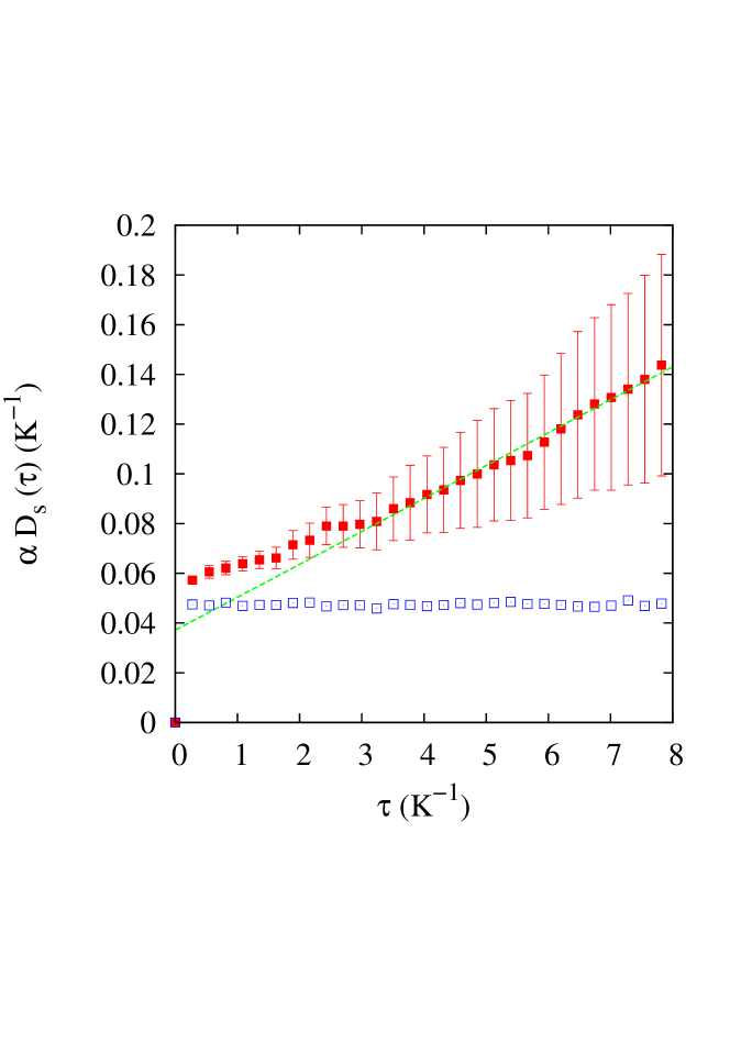
Figure 6: Estimator of the superfluid density for the first-layer 5-in-a-row supersolid H₂ phase at $\rho$ = 0.062 Å^-2 (open squares) and for a second-layer solid at total density $\rho$ = 0.167 Å^-2 (solid squares). The straight line is a linear least-squares fit to the latter set of data for the range $\tau>$ 3 K^-1.

Following exactly the same procedure outlined above for the case of ⁴He, we considered 7-in-a-row first-layer H₂ solids of different densities and deposited additional molecules on top of them. After that, we kept the arrangements with the minimum energy per particle for each total (first+second layer) densities. The second layer densities were calculated using as a surface adsorbate a cylinder of radius 9.42 Å. This is the mean distance of the molecules of the second layer to the axis of the tube. The minimum energies per molecule corresponded to a first-layer solid of $\rho_{s}$ = 0.100 Å^-2 with either a liquid ($c_{2}$ = 0 in Eq. 3) or a (super)solid ($c_{2}\neq$ 0) on top. In Fig. 7, we show those energies as a function of the inverse of the density. The $x$-range of that figure corresponds to the inverse of the experimental densities at which the H₂ is short of being promoted to a third layer on a flat substrate [27]. The solid data corresponds to a 15-in-a-row phase built in the same way that for the first-layer solids. The dotted line is a double tangent Maxwell construction between a single layer 7-in-a-row solid of density $\rho$ = 0.0975 Å^-2 and a two-layer solid of total density $\rho$ = 0.166 Å^-2. Both densities are within the error bars of the ones for a flat second H₂ absorbed on graphite [14].

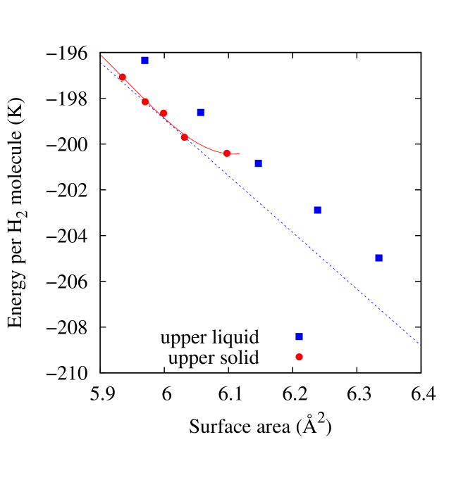
Figure 7: Energy per H₂ molecule as a function of the inverse of the total H₂ density. Solid squares, a two-layer structure with a liquid on top of a first-layer 7-in-a-row solid of density $\rho_{s}$ = 0.100 Å^-2. Solid circles, a 15-in-a-row upper solid on top of the same H₂ substrate. The dotted line is the Maxwell construction line between a single layer solid of $\rho$ = 0.0975 Å^-2 and a two-layer solid of $\rho$ = 0.166 Å^-2. The solid line is a third-order polynomial fit to the data intended exclusively as a guide-to-the eye.

In the same way as the second layer of H₂ on graphite at low densities, the 15-in-a-row H₂ on top of a nanotube is also a supersolid in a thin density slice. In Fig. 6 we can see (solid squares) the same superfluid estimator already described but applied only to the molecules on the second layer for a solid of total density $\rho$ = 0.167 Å^-2. For that arrangement, the slope corresponds to a supersolid density of 1.32 $\pm$ 0.05 %, larger but of the same order of magnitude as the value for the second layer of H₂ on graphite (0.41 $\pm$ 0.05 %).

IV Discussion

In this work, we have calculated the phase diagrams of ⁴He and H₂ on a single carbon nanotube. We chose the (5,5) one because is one of the thinnest experimentally obtained and its narrowness would make it a perfect candidate to see the differences between adsorption on a flat substrate and on a quasi-one dimensional one. Here, the dimensionality would be the only factor to take into account since the chemical composition of graphite, graphene, and carbon nanotubes is identical. Our simulation results suggest that the behavior of those species is quite similar on a cylinder and on its flat counterparts. There are, however, some minor differences.

⁴He is a supersolid at low densities. In this, its behavior is similar to that of a single sheet of ⁴He on top of graphene and graphite [12]. However, on a tube we have incommensurate structures instead of the $\sqrt{3}\times\sqrt{3}$ registered supersolid on the flat substrates. In any case, the superfluidity disappears upon ⁴He loading: both the incommensurate solid of 0.08 Å^-2 on graphene and the 6-in-a-row stable solids are normal. On the other hand, there is a significant difference in the promotion to a second layer. Even though on graphite there is a stable liquid in equilibrium with an incommensurate single-sheet solid, the density of that liquid is smaller than the one obtained in the present work (a total density of 0.163 Å^-2 [13] versus the value 0.181 Å^-2 of Table 1). In addition, we do not see a stable second-layer incommensurate solid up to the experimental density corresponding to a third layer promotion on graphite [9].

On the other hand, the behavior of H₂ on the selected nanotube is very similar to the one on top of graphene or graphite. The only difference is that, at very low densities, we have an incommensurate normal solid instead of the $\sqrt{3}\times\sqrt{3}$ normal structure on the flat adsorbents. We have also a promotion to a second layer supersolid at the same densities as in graphite [14]. The supersolid fraction at the lowest second layer densities is also comparable, albeit slightly larger than the one for graphite. This suggests that the behavior of H₂ depends more strongly on the strength of the H₂-H₂ interaction than in the dimensionality of the system and that it is probably necessary to disrupt the H₂ structure to observe new H₂ phases [31]. Another possible issue could be the quality of the empirical potential itself, and some alternatives to the Silvera-Goldman expression based on first-principles have been proposed [32, 33, 33, 34, 35, 36], some of them including three-body terms. However, the equation of state of solid $hcp$ H₂ obtained using those interactions is similar to the one calculated using the Silvera and Goldman potential [34] and in reasonably agreement with experiments. Moreover, a recent comparison between neutron scattering data for liquid and solid H₂ phases and simulations using the Silvera and Buck potentials suggests that both interactions are adequate to reproduce the experimental observables [37].

The superfluid fraction of the liquid ⁴He layer is one and the one of the solid H₂ layer is $\sim 0.01$. This large difference is mainly due to the different interaction between ⁴He atoms and H₂ molecules, the latter being much more attractive thus favoring the crystal phases. The superfluid fraction of this supersolid phase of H₂ may appear to be too small to be detected, but similar fractions were experimentally measured on the second layer of ⁴He on graphite [10] at temperatures low enough (0.5 K) to make our $T=0$ calculations relevant. The experiment [10] was made possible by using a specially designed double torsional oscillator able to disentangle the signals coming from the superfluid and elastic responses. On the other hand, a recent calculation [38] supports the existence of supersolidity in D₂ at very high pressures.