Bi-Drop: Enhancing Fine-tuning Generalization via Synchronous sub-net Estimation and Optimization

Abstract

Pretrained language models have achieved remarkable success in natural language understanding. However, fine-tuning pretrained models on limited training data tends to overfit and thus diminish performance. This paper presents Bi-Drop, a fine-tuning strategy that selectively updates model parameters using gradients from various sub-nets dynamically generated by dropout. The sub-net estimation of Bi-Drop is performed in an in-batch manner, so it overcomes the problem of hysteresis in sub-net updating, which is possessed by previous methods that perform asynchronous sub-net estimation. Also, Bi-Drop needs only one mini-batch to estimate the sub-net so it achieves higher utility of training data. Experiments on the GLUE benchmark demonstrate that Bi-Drop consistently outperforms previous fine-tuning methods. Furthermore, empirical results also show that Bi-Drop exhibits excellent generalization ability and robustness for domain transfer, data imbalance, and low-resource scenarios.

1 Introduction

In recent years, Natural Language Processing (NLP) has achieved significant progress due to the emergence of large-scale Pretrained Language Models (PLMs) (Devlin et al., 2018; Liu et al., 2019; Raffel et al., 2019; Clark et al., 2020). For downstream tasks, compared with training from scratch, fine-tuning pretrained models can usually achieve efficient adaptation and result in better performance. Despite the great success, fine-tuning methods still face challenges in maintaining generalization performance on downstream tasks - they tend to run into the overfitting issue when the training data is limited (Phang et al., 2018; Devlin et al., 2018; Lee et al., 2020).

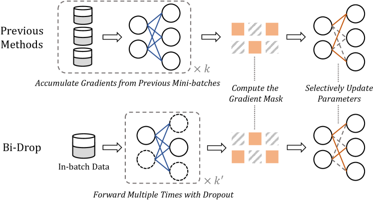
Figure 1: Comparisons between Bi-Drop and previous methods. Unlike previous methods that require multiple mini-batches of data to asynchronously determine the sub-net to optimize, Bi-Drop has a synchronous sub-net selection strategy with a higher data utility.

To improve the generalization ability of fine-tuning methods, many regularization techniques have been proposed (Chen et al., 2020; Aghajanyan et al., 2021; Wu et al., 2021; Xu et al., 2021; Yuan et al., 2022), such as sub-net optimization strategies like Child-Tuning${D}$ (Xu et al., 2021) and DPS (Zhang et al., 2022). Child-Tuning${D}$ selects a static sub-net for updating based on parameter importance estimated by Fisher Information (FI). As an improved variant of Child-Tuning_D, DPS dynamically decides the sub-net to be updated by estimating FI with multiple mini-batches of data. Although these FI-based methods achieve better generalization ability than vanilla fine-tuning, they still have two limitations: (1) hysteresis in sub-net updating: the sub-net preference is estimated with the model parameters in previous iterations and may be incompatible with the current update step; and (2) insufficient utility of training data: FI estimation requires cumulative gradients through multiple mini-batches, so these methods cannot fit in situations with data scarcity.

In this paper, we delve deeper into adaptive sub-net optimization strategies and propose Bi-Drop, a FI-free strategy for fine-tuning pretrained language models. Unlike Fisher information estimation, which requires cumulative gradients of mini-batches, Bi-Drop only relies on information in a single mini-batch to select the parameters to update. Specifically, Bi-Drop utilizes gradient information from different sub-nets dynamically generated by dropout in each mini-batch. As illustrated in Figure 1, within a single training step of Bi-Drop, a mini-batch will go through the forward pass multiple times and, due to the randomness introduced by dropout, yield various distinct sub-nets. We then apply a parameter selection algorithm with perturbation and scaling factors to stabilize the gradient updates. With this synchronous parameter selection strategy, Bi-Drop can selectively update model parameters according to the information from only the current mini-batch, and thus mitigate overfitting with a high utility of training data.

Extensive experiments on the GLUE benchmark demonstrate that Bi-Drop shows remarkable superiority over the state-of-the-art fine-tuning regularization methods, with a considerable margin of $0.53$ $\sim$ $1.50$ average score. Moreover, Bi-Drop consistently outperforms vanilla fine-tuning by $0.83$ $\sim$ $1.58$ average score across various PLMs. Further analysis indicates that Bi-Drop attains superb generalization ability for domain transfer and task transfer, and is robust for data imbalance and low-resource scenarios.

To sum up, our contributions are three-fold:

• We propose Bi-Drop, a step-wise sub-net optimization strategy that adaptively selects the updated sub-net based on the current mini-batch data. Compared with prior FI-based methods, Bi-Drop derives a more stable and robust training trajectory with simultaneous sub-net update and high utility of training data.

• With extensive experiments on various PLMs, we demonstrate that Bi-Drop achieves consistent and remarkable superiority over prior fine-tuning regularization methods.

• Further analysis shows that Bi-drop attains superb generalization ability for domain transfer and task transfer, and is robust for data imbalance and low-resource scenarios.

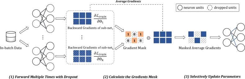
Figure 2: An overall illustration of Bi-Drop. Bi-Drop splits each training step into three sub-steps: (1) Multiple forward propagations: each mini-batch sample goes through the forward pass multiple times (denoted as $k$) with dropout; (2) sub-net selection: an advanced strategy is adopted to select the sub-net to be updated based on the gradients of distinct sub-nets generated by dropout; (3) Parameter updating: only the parameters of the selected sub-net are updated to mitigate overfitting.

2 Related Work

Pretrained Language Models

In recent years, the field of natural language processing (NLP) has witnessed significant advancements due to the development of large-scale pretrained language models (PLMs). The introduction of BERT (Devlin et al., 2018) sparked a continuous emergence of various pre-trained models, including RoBERTa (Liu et al., 2019), ELECTRA (Clark et al., 2020), XLNet (Yang et al., 2019), GPT-2 (Radford et al., 2019), and GPT-3 (Brown et al., 2020), which have brought remarkable improvements in model structures and scales. Until now, fine-tuning is still one of the most popular approaches to adapting large pretrained language models to downstream tasks.

Models	Sub-net Granularity	Hyste- resis	Data Depend.
Child-TuningD	task-wise	Yes	Yes
DPS	cycle-wise	Yes	Yes
Bi-Drop	step-wise	No	No

Table 1: Comparison of Bi-Drop with prior FI-based sub-net optimization methods. “cycle-wise” refers to the granularity that includes multiple mini-batches of data.

Regularization Methods for Fine-tuning

Large-scale PLMs are prone to over-fitting Phang et al. (2018); Devlin et al. (2018) and exhibit inadequate generalization ability when fine-tuned with limited training data Aghajanyan et al. (2021); Mahabadi et al. (2021), resulting in degraded performance. To tackle this issue, various regularization techniques have been suggested to enhance the generalization capacity of models, including advanced dropout alternatives Wan et al. (2013); Wu et al. (2021), applying adversarial perturbations Aghajanyan et al. (2021); Wu et al. (2022); Yuan et al. (2022) and constrained regularization methods DauméIII (2007); Chen et al. (2020). In recent years, Child-tuning Xu et al. (2021) and DPS Zhang et al. (2022) propose to estimate parameter importance based on Fisher Information (FI) and selectively optimize a sub-net during fine-tuning to mitigate overfitting.

FI-based methods have a strong dependence on the training data and exhibit hysteresis in sub-net updating. As shown in Table 1, compared with prior FI-based methods, Bi-Drop introduces a step-wise sub-net optimization strategy that adaptively selects the sub-net to be updated based on the current mini-batch. It is worth noting that, as a model-agnostic technique, Bi-Drop is orthogonal to most previous fine-tuning methods, which could further boost the model’s performance.

3 Methodology

3.1 Background

We first introduce the paradigm of sub-net optimization by giving general formulations of the backpropagation during the vanilla fine-tuning and Child-Tuning_D. We denote the parameters of the model at $t$-th iteration as $\bm{\theta}_{t}=\{\theta_{t,i}\}_{i=1}^{n}$, where $\theta_{t,i}$ represent the $i$-th element of $\bm{\theta}_{t}$ at the $t$-th training iteration. $\bm{\theta}_{0}$ denotes the parameter matrix of the pre-trained model. The vanilla fine-tuning adopts Stochastic Gradient Descent (SGD) to all the model parameters, formally:

$$\bm{\theta}_{t+1}=\bm{\theta}_{t}-\eta\frac{\partial\mathcal{L}\left(\bm{\theta}_{t}\right)}{\partial\bm{\theta}_{t}}$$ (1)

where $\mathcal{L}$ represents the training loss within a batch; $\eta$ is the learning rate. Instead of fine-tuning the entire network, Child-Tuning_D proposes to only optimize a subset of parameters (i.e., the sub-net). It first adopts the Fisher Information (FI) to estimate the relative importance of the parameters for a specific downstream task, which can be formulated as:

$$F(\bm{\theta}_{0})=\sum_{j=1}^{|\mathcal{D}|}\left(\frac{\partial\mathcal{L}\left(\bm{\theta}_{0}\right)}{\partial\bm{\theta}_{0}}\right)^{2}$$ (2)

$$\bm{M}_{CT_{D}}=F(\bm{\theta}_{0})>\operatorname{sort}\left(F(\bm{\theta}_{0})\right)_{p}$$ (3)

where $\mathcal{D}$ is the training data, $F(\bm{\theta}_{0})$ denotes the fisher information matrix of the pretrained parameters; $\operatorname{sort}(\cdot)_{p}$ represents the highest value of $p$ percentile in $F(\bm{\theta}_{0})$ after sorting in ascending order; $\bm{M}_{CT_{D}}$ is a mask matrix that is the same-sized as $\bm{\theta}_{0}$. During fine-tuning, Child-Tuning_D only optimizes the selected sub-net in $M_{CT_{D}}$:

$$\bm{\theta}_{t+1}=\bm{\theta}_{t}-\eta\frac{\partial\mathcal{L}\left(\bm{\theta}_{t}\right)}{\partial\bm{\theta}_{t}}\bm{M}_{CT_{D}}$$ (4)

3.2 Bi-Drop

As introduced in Section 3.1, Child-Tuning_D only optimizes an unchanged sub-net during fine-tuning and ignores the update of other parameters, which may degrade the model’s performance on downstream tasks. In this section, we offer a detailed introduction to our proposed method, Bi-Drop, which selects the updated parameters adaptively at each fine-tuning step. Specifically, Bi-Drop splits each training step into three sub-steps: (1) multiple forward propagations, (2) sub-net selection, and (3) parameter updating. We provide a pseudo-code of Bi-Drop in Algorithm 1.

3.2.1 Multiple Forward Propagations

Instead of prior FI-based methods that require accumulated gradients to measure the parameter importance, Bi-Drop leverages distinct sub-nets generated by dropout to select the sub-net to be updated. Inspired by Wu et al. (2021), given the training data $\mathcal{D}=\{(x_{i},y_{i})\}_{i=1}^{m}$, at each training step, we feed $x_{i}$ to the model multiple times in the forward pass with different dropouts, and obtain their gradients correspondingly:

$$\mathbf{g}_{t}^{(j)}=\frac{\partial\mathcal{L}(\bm{\theta}_{t}^{(j)})}{\partial\bm{\theta}_{t}^{(j)}},\quad j=1,2,...,k$$ (5)

where $\bm{\theta}_{t}^{(j)}$ and $\mathbf{g}_{t}^{(j)}$ represents the parameters of the $j$-th forward pass and its corresponding gradients. $k$ denotes the number of forward passes, i.e., the number of distinct sub-nets with different dropouts.

Algorithm 1 Bi-Drop for Adam Optimizer

1:$\bm{\theta}_{0}$: initial pretrained weights; $\mathcal{L}(\bm{\theta})$: stochastic objective function with parameters $\bm{\theta}$; $\beta_{1},\beta_{2}\in[0,1)$: exponential decay rates for the moment estimates; $\eta$: learning rate;

2:initialize timestep $t\leftarrow 0$, first moment vector $\mathbf{m}_{0}\leftarrow\mathbf{0}$, second moment vector $\mathbf{v}_{0}\leftarrow\mathbf{0}$

3:while not converged do

4:     $t\leftarrow t+1$

5:      // Multiple forward propagations

6:     $\mathbf{g}_{t}^{(j)}\leftarrow\frac{\partial\mathcal{L}(\bm{\theta}_{t}^{(j)})}{\partial\bm{\theta}_{t}^{(j)}},\quad j=1,2,...,k$

7:      // Sub-net selection

8:     $\bm{M}_{t}\leftarrow\text{SelectSubNetwork}(\mathbf{g}_{t})$

9:      // Gradients Updating

10:     $\mathbf{g}_{t}\leftarrow\mathbf{g}_{t}\odot\bm{M}_{t}$

11:     $\mathbf{m}_{t}\leftarrow\beta_{1}\cdot\mathbf{m}_{t-1}+(1-\beta_{1})\cdot\mathbf{g}_{t}$

12:     $\mathbf{v}_{t}\leftarrow\beta_{2}\cdot\mathbf{v}_{t-1}+(1-\beta_{2})\cdot\mathbf{g}^{2}_{t}$

13:     $\hat{\mathbf{m}}_{t}\leftarrow\mathbf{m}_{t}/(1-\beta_{1}^{t})$

14:     $\hat{\mathbf{v}}_{t}\leftarrow\mathbf{v}_{t}/(1-\beta_{2}^{t})$

15:      // Update weights

16:     $\mathbf{w}_{t}\leftarrow\mathbf{w}_{t-1}-\eta\cdot\hat{\bm{m}}_{t}/(\sqrt{\hat{\bm{v}}_{t}}+\epsilon)$

17:end while

18:return $\mathbf{w}_{t}$

3.2.2 Sub-net Selection

In this subsection, we introduce our sub-net selection strategy, which estimates the relevant importance of parameters based on the gradients of distinct sub-nets generated by different dropouts. Concretely, our strategy is based on two estimation factors: the perturbation factor and the scaling factor.

Perturbation Factor

We propose the perturbation factor, which estimates the importance of parameters according to their stability with different dropouts in the forward pass. We point out that various sub-nets generated by dropout can be viewed as adversarial perturbations to the vanilla model. The perturbation factor is formalized as follows:

$$\bm{\mu}_{t}=\frac{1}{k}\sum_{j=1}^{k}\mathbf{g}_{t}^{(j)}$$ (6)

$$\mathbf{F}_{\text{per}}(\bm{\theta}_{t})=\left|\bm{\mu}_{t}\right|\cdot\left[\sum_{j}\left(\mathbf{g}_{t}^{(j)}-\bm{\mu}_{t}\right)^{2}\right]^{-\frac{1}{2}}$$ (7)

where $\bm{\mu}_{t}$ is the average gradients of parameters. $\mathbf{F}_{\text{per}}$ measures the stability of parameters by both considering the mean and variance of gradients with adversarial perturbations, i.e. sub-nets with consistently larger gradients and smaller variances are more favorable by this factor.

Scaling Factor

We further propose the scaling factor as a regularization term. This factor measures the ratio of the average parameter gradients to the original parameters. Parameters whose gradient scale is much smaller than the original parameters will not be updated, which is similar in spirit to gradient clipping.

$$\mathbf{F}_{\text{sca}}(\bm{\theta}_{t})=\left|\bm{\mu}_{t}\right|\cdot\left|\bm{\theta}_{t}\right|^{-1}$$ (8)

3.2.3 Parameter Updating

Following prior work Xu et al. (2021); Zhang et al. (2022), we derive a step-wise mask matrix $\bm{M}_{t}$ filtered by selecting the highest value of $p$ percentile measured by the aforementioned two estimation factors.

$$\mathbf{F}_{\text{final}}(\bm{\theta}_{t})=\mathbf{F}_{\text{per}}(\bm{\theta}_{t})\cdot\mathbf{F}_{\text{sca}}(\bm{\theta}_{t})$$ (9)

$$\bm{M}_{t}=\mathbf{F}_{\text{final}}(\bm{\theta}_{t})>\operatorname{sort}\left(\mathbf{F}_{\text{final}}(\bm{\theta}_{t}))\right)_{p}$$ (10)

Then, we utilize $\bm{M}_{t}$ to update the sub-net which consists of important parameters at each training step. We denote the formulation by simply replacing Eq.4 with our step-wise mask matrix $\bm{M}_{t}$:

$$\bm{\theta}_{t+1}=\bm{\theta}_{t}-\eta\bm{\mu}_{t}\cdot\bm{M}_{t}$$ (11)

Method	CoLA	MRPC	RTE	STS-B	Avg	$\Delta$
Vanilla	63.76(65.55)	90.41(91.91)	70.97(74.01)	89.70(90.58)	78.71(80.51)	0.00
Weight Decay	63.70(65.53)	90.89(91.98)	72.24(74.37)	89.66(90.22)	79.12(80.53)	+0.41(0.02)
Top-K Tuning	63.89(65.37)	91.09(92.05)	72.84(75.17)	89.64(90.83)	79.37(80.86)	+0.66(0.35)
Mixout	64.05(65.41)	91.19(92.05)	72.32(75.52)	89.89(90.42)	79.36(80.85)	+0.65(0.34)
RecAdam	64.09(65.35)	90.88(91.89)	72.48(74.30)	89.67(90.62)	79.28(80.54)	+0.57(0.03)
ChildTuningD	64.25(65.81)	91.19(92.20)	72.35(76.53)	90.18(90.88)	79.49(81.36)	+0.78(0.85)
R3F	64.88(66.33)	91.55(92.28)	72.42(74.37)	89.70(90.58)∗	79.64(80.89)	+0.93(0.38)
DPSmix	64.40(66.21)	91.05(92.17)	72.88(75.81)	90.47(91.02)	79.70(81.30)	+0.99(0.79)
R-Drop	64.83(66.79)	91.76(92.17)	73.12(76.53)	90.14(90.42)	79.96(81.48)	+1.25(0.97)
Bi-Drop	64.94(66.69)	91.79(92.68)	73.79(77.61)	90.59(91.04)	80.26(82.01)	+1.55(1.50)

Table 2: Comparison between Bi-Drop with prior fine-tuning methods. We report the mean (max) results of 10 random seeds. The best results are bold. Note that since R3F is not applicable to regression, the result on STS-B (marked with ^∗) remains the same as vanilla. Bi-Drop achieves the best performance compared with other methods.

4 Experiments

4.1 Datasets

GLUE Benchmark

Following previous work (Lee et al., 2020; Dodge et al., 2020; Zhang et al., 2021), we conduct extensive experiments on the GLUE benchmark, including natural language inference (RTE, QNLI, MNLI), paraphrase and similarity (MRPC, STS-B, QQP), linguistic acceptability (CoLA), and sentiment classification (SST-2). We include the detailed statistics and metrics of the datasets in Appendix A. Since the test results are only accessible online with limited submission times, we follow prior studies (Phang et al., 2018; Lee et al., 2020; Aghajanyan et al., 2021; Dodge et al., 2020; Xu et al., 2021; Zhang et al., 2022) that fine-tune the pretrained model on the training set and report the results on the development sets using the last checkpoint.

NLI Datasets

We also evaluate the generalization ability of Bi-Drop on several Natural Language Inference (NLI) tasks, including SNLI (Bowman et al., 2015), MNLI (Williams et al., 2018), MNLI-M (Williams et al., 2018) and SICK (Marelli et al., 2014). We report all results by Accuracy on the development sets consistent with GLUE.

4.2 Baselines

Besides the vanilla fine-tuning method, we mainly compare Bi-Drop with the following baselines:

Mixout (Lee et al., 2020) is a fine-tuning technique that stochastically replaces the parameters with their pretrained weight based on the Bernoulli distribution. R3F (Aghajanyan et al., 2021) is a fine-tuning strategy motivated by trust-region theory, which injects noise sampled from either a normal or uniform distribution into the pre-trained representations. R-Drop (Wu et al., 2021) minimizes the bidirectional KL-divergence to force the output distributions of two sub-nets sampled by dropout to be consistent with each other. Child-Tuning_D (Xu et al., 2021) selects the task-relevant parameters as the sub-net based on the Fisher information and only updates the sub-net during fine-tuning. DPS (Zhang et al., 2022) is a dynamic sub-net optimization algorithm based on Child-Tuning_D. It estimates Fisher information with multiple mini-batches of data and selects the sub-net adaptively during fine-tuning.

For reference, we also show other prior fine-tuning techniques in our main experimental results, such as Weight Decay DauméIII (2007), Top-K Tuning Houlsby et al. (2019) and RecAdam Chen et al. (2020).

Method	BERTbase					Robertabase
	CoLA	MRPC	RTE	STS-B	Avg	CoLA	MRPC	RTE	STS-B	Avg
Vanilla	57.67	90.38	69.57	89.35	76.74	59.45	91.94	76.28	90.60	79.57
Bi-Drop	60.76	91.01	71.73	89.78	78.32	61.28	92.40	78.99	91.00	80.92
Method	BERTlarge					Robertalarge
	CoLA	MRPC	RTE	STS-B	Avg	CoLA	MRPC	RTE	STS-B	Avg
Vanilla	63.76	90.41	70.97	89.70	78.71	66.01	92.56	84.51	92.05	83.78
Bi-Drop	64.94	91.79	73.79	90.50	80.26	68.03	92.95	86.10	92.36	84.86
Method	DeBERTalarge					ELECTRAlarge
	CoLA	MRPC	RTE	STS-B	Avg	CoLA	MRPC	RTE	STS-B	Avg
Vanilla	65.18	92.32	85.60	91.64	83.69	70.02	92.94	88.37	91.91	85.81
Bi-Drop	66.91	92.88	86.72	92.33	84.71	71.29	93.68	88.98	92.61	86.64

Table 3: Comparison between Bi-Drop and vanilla fine-tuning applied to six widely-used large-scale PLMs. We report the mean results of 10 random seeds. Average scores on all tasks are underlined. The best results are bold. It shows that Bi-Drop yields consistent improvements across all tasks among different PLMs.

4.3 Experiments Setup

We conduct our experiments based on the HuggingFace transformers library (Wolf et al., 2020) and follow the default hyper-parameters and settings unless noted otherwise. We report the averaged results over 10 random seeds. Other detailed experimental setups are presented in Appendix B.

Datasets	SNLI					MNLI
	Vanilla	CTD	R-Drop	DPS	Bi-Drop	Vanilla	CTD	R-Drop	DPS	Bi-Drop
MNLI	64.53	64.16	64.51	64.70	66.88	75.78	76.27	76.85	75.48	76.63
MNLI–m	66.11	66.30	66.59	67.29	68.49	77.31	77.30	77.93	77.45	77.98
SNLI	83.37	83.53	83.59	82.95	83.62	70.87	70.76	71.48	71.56	71.63
SICK	52.59	53.73	53.59	55.89	54.28	53.27	55.35	54.21	54.81	54.93
Avg	61.08	61.40	61.56	62.63	63.22	67.15	67.80	67.87	67.94	68.18
$\Delta_{avg}$	–	$\uparrow$ 0.32	$\uparrow$ 0.48	$\uparrow$ 1.55	$\uparrow$ 2.14	–	$\uparrow$ 0.65	$\uparrow$ 0.72	$\uparrow$ 0.79	$\uparrow$ 1.03

Table 4: Evaluation for out-of-domain generalization.The models are trained on MNLI/SNLI and tested on out-of-domain data. Average scores are computed excluding in-domain results (underlined). The best results are bold. Bi-Drop can better maintain the out-of-domain generalization ability of the model.

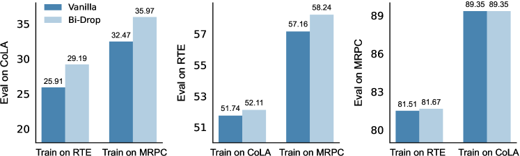
Figure 3: Evaluation for task generalization. The model is fine-tuned on a specific task among MRPC, CoLA, RTE and transferred to the other two tasks. Bi-Drop can be more generalizable.

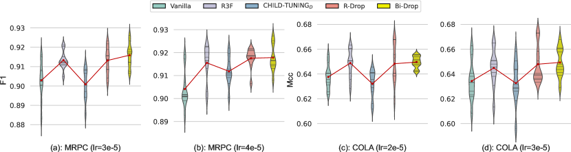
Figure 4: Results of Bi-Drop across four experimental settings. Each method includes a violin plot for 10 random runs. Compared with other methods, the shorter and thicker violin plot of Bi-Drop proves its better stability.

4.4 Results on GLUE

Comparison with Prior Methods

We compare Bi-Drop with various prior fine-tuning methods based on BERT_large and report the mean (and max) scores on GLUE benchmark in Table 2, following Lee et al. (2020) and Xu et al. (2021). The results indicate that Bi-Drop yields the best average performance across all tasks, showing its effectiveness. Moreover, the average of the maximum scores attained by Bi-Drop is superior to that of other methods, providing further evidence of the effectiveness of Bi-Drop. We also conducted the same experiment on Roberta_large, and the details can be found in Appendix E.

Comparison with Vanilla Fine-tuning

We show the experimental results of six widely used large-scale PLMs on the GLUE Benchmark in Table 3. The results show that Bi-Drop outperforms vanilla fine-tuning consistently and significantly across all tasks performed on various PLMs. For instance, Bi-Drop achieves an improvement of up to 1.58 average score on BERT_base and 1.35 average score on Roberta_base. The results highlight the universal effectiveness of Bi-Drop in enhancing the fine-tuning performance of PLMs. Additionally, because Bi-Drop forward-propagate twice, we present an additional study of the baseline with doubled batch size in Appendix D.

Method	CoLA	MRPC	RTE	Avg
Noise Ratio: 5%
vanilla	61.39	90.24	69.78	73.80 ($\downarrow$ 1.25)
$\text{CT}_{D}$	61.66	90.39	71.47	74.51 ($\downarrow$ 1.77)
R-Drop	62.33	91.21	73.16	75.57 ($\downarrow$ 1.00)
Bi-Drop	62.29	91.85	73.57	75.90 ($\downarrow$ 0.94)
Noise Ratio: 10%
vanilla	59.35	89.78	68.51	72.55 ($\downarrow$ 2.50)
$\text{CT}_{D}$	61.56	89.88	69.78	73.72 ($\downarrow$ 2.56)
R-Drop	61.12	91.10	71.36	74.53 ($\downarrow$ 2.04)
Bi-Drop	61.65	91.12	71.96	74.91 ($\downarrow$ 1.93)
Noise Ratio: 15%
vanilla	58.96	88.10	68.14	71.73 ($\downarrow$ 3.32)
$\text{CT}_{D}$	59.99	88.10	68.88	72.32 ($\downarrow$ 3.96)
R-Drop	60.80	89.26	69.55	73.20 ($\downarrow$ 3.36)
Bi-Drop	60.08	89.73	70.88	73.56 ($\downarrow$ 3.28)

Method	CoLA	MRPC	RTE	Avg
Reduction Ratio: 70%
Vanilla	81.12	78.88	27.71	62.57 ( – )
CTD	83.10	79.50	28.14	63.58 ($\uparrow$ 1.01)
R-Drop	81.37	76.46	32.61	63.48 ($\uparrow$ 0.91)
Bi-Drop	81.88	80.17	37.66	66.57 ($\uparrow$ 4.00)
Reduction Ratio: 60%
Vanilla	83.30	83.98	39.32	68.87 ( – )
CTD	85.78	84.55	37.65	69.33 ($\uparrow$ 0.46)
R-Drop	83.55	85.07	43.51	70.71 ($\uparrow$ 1.84)
Bi-Drop	84.33	85.35	49.62	73.10 ($\uparrow$ 4.23)
Reduction Ratio: 50%
Vanilla	86.07	87.40	45.27	72.91 ( – )
CTD	87.98	87.64	50.78	75.47 ($\uparrow$ 2.56)
R-Drop	86.04	88.89	55.73	76.89 ($\uparrow$ 3.98)
Bi-Drop	86.73	89.61	58.27	78.20 ($\uparrow$ 5.29)

Table 5: Left: Robustness to label noise. The noise ratio is the percentage of training instances whose labels are transferred to incorrect labels. Right: Robustness to data imbalance. We reduce the number of instances labeled 1 by 70%/60%/50% in the training set and test the accuracy of instances labeled 1 (as the minority class) in the validation set. Bi-Drop can maintain more robust representations compared with other fine-tuning methods.

4.5 Out-of-Domain Generalization

We further evaluate the generalization ability of Bi-Drop on a widely used experimental setting in prior research (Aghajanyan et al., 2021; Xu et al., 2021; Zhang et al., 2022): out-of-domain generalization. In detail, we finetune BERT_large with different strategies on $5k$ subsampled MNLI and SNLI datasets respectively, and directly evaluate the fine-tuned model on other NLI datasets. The experimental results in Table 4 illustrate that Bi-Drop outperforms vanilla fine-tuning and prior methods across various datasets. Specifically, compared with other fine-tuning methods on SNLI, Bi-Drop demonstrates consistent and substantial improvement, with an average score increase of 2.14. In particular, Bi-Drop achieves an improvement of 2.35 on MNLI task and 2.38 on MNLI-m task. For models trained on MNLI, Bi-Drop also consistently outperforms prior methods, with an average improvement of 1.03 score. The experimental results indicate that Bi-Drop encourages the model to learn deeper and more generic semantic features and alleviate superficial biases of specific tasks, which improves the model’s generalization ability.

4.6 Task Generalization

We also evaluate the generalization ability of fine-tuned models following the experimental setting of Aghajanyan et al. (2021) and Xu et al. (2021), which freezes the representations of the model fine-tuned on one task and only trains the linear classifier on the other task. Specifically, we finetune BERT_large among one task selected among MRPC, CoLA, and RTE and then transfer the model to the other two tasks. Figure 3 shows that Bi-Drop consistently outperforms vanilla fine-tuning when the fine-tuned model is transferred to other tasks. In particular, Bi-Drop improves by 3.50 and 3.28, when models trained on MRPC and RTE respectively are evaluated on CoLA. The results further verify the conclusion that Bi-Drop helps models learn more generalizable representations, compared with the vanilla fine-tuning approach.

5 Analysis

Datasets	0.5K				1K
	Vanilla	CTD	DPS	Bi-Drop	Vanilla	CTD	DPS	Bi-Drop
CoLA	36.23	40.77	41.87	44.78	48.92	51.63	52.89	54.76
MRPC	81.33	81.95	83.29	83.18	83.90	84.62	85.03	85.44
RTE	58.87	59.27	59.16	60.04	62.17	63.85	64.92	66.96
STS-B	82.60	82.79	83.41	85.19	85.91	86.92	87.26	87.53
SST-2	86.11	88.19	89.08	89.38	89.95	89.88	90.44	90.41
QNLI	78.76	79.32	79.27	80.48	82.49	83.65	83.86	84.35
QQP	71.88	73.43	74.22	74.61	77.65	78.57	78.79	79.01
MNLI	46.44	45.74	47.63	50.79	56.55	60.96	59.47	61.25
Avg	67.78	68.93	69.74	71.06	73.44	75.01	75.33	76.21
$\Delta_{avg}$	–	$\uparrow$ 1.15	$\uparrow$ 1.96	$\uparrow$ 3.28	–	$\uparrow$ 1.57	$\uparrow$ 1.89	$\uparrow$ 2.77

Table 6: Comparison between Bi-Drop and prior sub-net optimization strategies with varying low-resource scenarios (0.5K, 1K). We report the results of 10 random seeds and the best results are bold. Bi-Drop performs better than other methods in low-resource scenarios.

Method	CoLA	MRPC	RTE	STS-B	Avg	$\Delta$
Bi-Drop (gavg + ESS)	64.94	91.79	73.79	90.59	80.26	+1.55
gavg + Perturbation Factor	64.71	91.67	73.21	90.36	79.99	+1.28
gavg + Scaling Factor	64.38	91.63	72.96	90.41	79.85	+1.14
gavg + RSS	64.24	90.96	71.73	90.25	79.30	+0.59
gavg	63.82	91.26	71.16	89.81	79.01	+0.30
Vanilla	63.76	90.41	70.97	89.70	78.71	0.00

Table 7: Ablation results. ESS represents our Effective Sub-net Selection strategy using both factors Perturbation and Scaling. RSS stands for Random Sub-net Selection strategy. Both our sub-net selection strategy and gradient averaging strategy are effective.

5.1 Stability to Random Seeds

We further investigate the stability properties of fine-tuned models. Figure 4 shows the output distributions of models with four experimental settings and across 10 random seeds. The results demonstrate that Bi-Drop outperforms other strategies in terms of average performance, and also exhibits greater stability by achieving more consistent results across 10 random seeds with lower variance.

5.2 Robustness Analysis

Recent research has brought to light that the vanilla fine-tuning approach is prone to deception and vulnerability in many aspects. In this study, we assess the robustness of Bi-Drop by designing evaluation tasks that focus on two common scenarios, aiming to examine its ability to withstand various forms of perturbations while maintaining its robustness.

Robustness to Label Noise

Due to the inherent limitations of human annotation, widely-used large-scale datasets inevitably contain a certain amount of incorrect labels Vasudevan et al. (2022). To investigate the robustness of Bi-Drop to label noise, we conduct simple simulation experiments on RTE, MRPC, and CoLA by randomly corrupting a predetermined fraction of labels with erroneous values. We evaluate the robustness of various fine-tuning methods trained on noisy data. The results shown in the left panel of Table 5 demonstrate that Bi-Drop achieves consistent superiority to other fine-tuning methods on noisy data. Furthermore, we conducted a comparison of model performance degradation across varying noise ratios. We calculated the degradation and presented it in brackets, as compared with Table  2. It indicates that Bi-Drop has the smallest performance drop compared with other fine-tuning methods. These results collectively demonstrate that Bi-Drop is more robust to label noise than prior methods.

Robustness to Data Imbalance

Minority class refers to the class that owns insufficient instances in the training set. In this section, we strive to explore the robustness of diverse fine-tuning approaches for the minority class by carrying out experiments on synthetic RTE, MRPC, and CoLA datasets. The experimental results are illustrated in the right panel of Table 5, which shows that Bi-Drop significantly outperforms other fine-tuning methods. Bi-Drop achieves up to 4.00, 4.23, and 5.29 average score improvements on 30%, 40%, and 50% reduction ratios respectively, outperforming other fine-tuning methods at lower reduction ratios and showcasing its robustness towards the minority class.

5.3 Performance in Low-Resource Scenarios

As illustrated in Section 1 and 2, compared with prior FI-based sub-net optimization methods that have a strong dependence on the training data, Bi-Drop proposes a step-wise sub-net selection strategy, which chooses the optimized parameters with the current mini-batch. In this section, we conduct extensive experiments to analyze how this dependency affects the performance of models. Concretely, we adopt various fine-tuning methods on BERT_large with a limited amount of training data. The results are illustrated in Table 6. As the data amount decreases from 1.0K to 0.5K, the average improvement score of Child-Tuning_D over vanilla fine-tuning decreases from 1.57 to 1.15, while its improved variant DPS maintains a relatively stable improvement. But Bi-Drop improves the average improvement score from 2.77 to 3.28. The results indicate the superiority of Bi-Drop over prior methods in low-resource scenarios.

5.4 Ablation Study

To evaluate the effectiveness of our proposed fine-tuning strategy, we conduct an ablation study in Table 7. The results show that both our sub-net selection strategy and gradient averaging strategy contribute to the performance improvement of Bi-Drop.

6 Conclusion

In this work, we propose a new sub-net optimization technique for large-scale PLMs, named Bi-Drop, which leverages the gradients of multiple sub-nets generated by dropout to select the updated parameters. Extensive experiments on various downstream tasks demonstrate that Bi-Drop achieves consistent and remarkable improvements over vanilla fine-tuning and prior excellent approaches by a considerable margin, across various model architectures. Further analysis indicates the generalizability and robustness of Bi-Drop over transferring, data imbalance and low-resource experiments.

7 Limitations

We propose a novel and effective fine-tuning method, Bi-Drop, which achieves a considerable performance improvement in downstream tasks. However, similar to some previous studies(Jiang et al., 2020; Aghajanyan et al., 2021; Wu et al., 2021), Bi-Drop requires multiple forward propagations, which makes its training time efficiency not good enough compared with the vanilla fine-tuning method.

Appendix

Appendix A GLUE Benchmark Datasets

In this paper, we conduct experiments on datasets in GLUE benchmark Wang et al. (2019). The statistical information of the GLUE benchmark is shown in Table 8.

Dataset	#Train	#Dev	Metrics
Single-sentence Tasks
CoLA	8.5k	1.0k	Matthews Corr
SST-2	67k	872	Accuracy
Inference
RTE	2.5k	277	Accuracy
QNLI	105k	5.5k	Accuracy
MNLI	393k	9.8k	Accuracy
Similarity and Paraphrase
MRPC	3.7k	408	F1
STS-B	5.7k	1.5k	Spearman Corr
QQP	364k	40k	F1

Table 8: Statistics and metrics of eight datasets used in this paper form GLUE benchmark.

Model	Dataset	Batch Size	Epochs/Steps	Warmup Ratio/Steps
BERT	all	16	3 epochs	10%
Roberta	CoLA	16	5336 steps	320 steps
	RTE	16	2036 steps	122 steps
	MRPC	16	2296 steps	137 steps
	STS-B	16	3598 steps	214steps
ELECTRA	CoLA	32	3 epochs	10%
	RTE	32	10 epochs	10%
	MRPC	32	3 epochs	10%
	STS-B	32	10 epochs	10%
DeBERTa	CoLA	32	6 epochs	100 steps
	RTE	32	6 epochs	50 steps
	MRPC	32	6 epochs	10 steps
	STS-B	32	4 epochs	100 steps

Table 9: Hyperparameters settings for different pretrained models on variant tasks. These settings are reported in their official repository for best practice.

Appendix B Experimental Details

In this paper, we fine-tune different large pretrained language models with Bi-Drop, including BERT_BASE, BERT_LARGE, RoBERTa_BASE, RoBERTa_LARGE, DeDERTa_LARGE, and ELECTRA_LARGE. The training epochs/steps, batch size, and warmup steps are listed in Table 9.

For the glue dataset, our maximum length is set as $128$. We use grid search for learning rate from $\left\{1\text{e-}5,2\text{e-}5,\dots,1\text{e-}4\right\}$. For Bi-Drop, we use grid search for dropout rate from $\left\{0.05,0.1\right\}$. The number of forward passes is fixed to two($k$ = 2). We conduct all the experiments on a single A40 GPU.

Appendix C Hyper-Parameter Analysis

Bi-Drop uses two dropout techniques. In order to analyze the impact of the dropout rate on the experimental results, a simple analysis experiment was done here. In order to make the comparison fair, all the parameters except the dropout rate are kept the same in the experiment. For simplicity, the dropout values are the same twice. The experimental results are shown in 5. It can be seen that different datasets have different preferences for dropout values. CoLA and RTE achieve the best results when the dropout value is 0.05; while MRPC achieves the best results when the dropout value is 0.1; STSB is insensitive to the dropout value until the dropout value is less than 0.1.

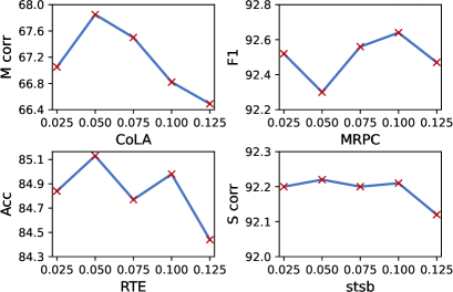
Figure 5: The effect of dropout rate on experimental results

Appendix D Batch Size Doubled Training

We implement Bi-Drop by repeating the input data twice and forward-propagating twice. This is similar to doubling the batch size at each step. The difference is that half of the data is the same as the other half, and directly doubling the batch size, the data in the same mini-batch is all different. So for a fair comparison, we experimented with directly doubling the batch size. So for a fair comparison, we experimented with directly doubling the batch size. The experimental results are shown in Table 10, results show that directly doubling the batch size has basically no improvement, and Bi-Drop is significantly better than directly doubling the batch size.

Method	CoLA	MRPC	RTE	STS-B	Avg
Vanilla	57.67	90.38	69.57	89.35	76.74
Vanilla(double bsz)	57.69	90.08	69.85	89.55	76.79
Bi-Drop	60.76	91.01	71.73	89.78	78.32

Table 10: Comparison of Bi-Drop and directly doubling the batch size. Bi-Drop is significantly better than directly doubling the batch size.

Appendix E Comparison with Prior Methods on Roberta_large

We compare Bi-Drop with various prior fine-tuning methods based on BERT_large and report the mean (and max) scores on GLUE benchmark in Table 11, following Lee et al. (2020) and Xu et al. (2021).

Method	CoLA	MRPC	RTE	STS-B	Avg	$\Delta$
Vanilla	66.01(68.03)	92.56(93.66)	84.51(86.28)	92.05(92.22)	83.78(85.05)	0.00
ChildTuningD	66.82(68.21)	92.67(93.58)	85.89(87.72)	92.36(92.53)	84.44(85.51)	+0.66(0.46)
DPSmix	66.86(68.53)	92.51(93.89)	85.37(87.72)	92.47(92.73)	84.30(85.72)	+0.52(0.67)
R-Drop	67.26(69.63)	92.47(93.62)	85.44(87.63)	92.42(92.58)	84.40(85.87)	+0.62(0.82)
Bi-Drop	68.03(70.89)	92.95(94.66)	86.10(88.09)	92.36(92.58)	84.86(86.56)	+1.08(1.51)

Table 11: Comparison between Bi-Drop with prior fine-tuning methods. We report the mean (max) results of 10 random seeds. The best results are bold. Note that since R3F is not applicable to regression, the result on STS-B (marked with ^∗) remains the same as vanilla. Bi-Drop achieves the best performance compared with other methods.

References

- Aghajanyan et al. (2021) Armen Aghajanyan, Akshat Shrivastava, Anchit Gupta, Naman Goyal, Luke Zettlemoyer, and Sonal Gupta. 2021. Better fine-tuning by reducing representational collapse. In ICLR.
- Bowman et al. (2015) Samuel R. Bowman, Gabor Angeli, Christopher Potts, and Christopher D. Manning. 2015. A large annotated corpus for learning natural language inference. In Proceedings of the 2015 Conference on Empirical Methods in Natural Language Processing, EMNLP 2015, Lisbon, Portugal, September 17-21, 2015, pages 632–642. The Association for Computational Linguistics.
- Brown et al. (2020) Tom Brown, Benjamin Mann, Nick Ryder, Melanie Subbiah, Jared D Kaplan, Prafulla Dhariwal, Arvind Neelakantan, Pranav Shyam, Girish Sastry, Amanda Askell, et al. 2020. Language models are few-shot learners. In NeurIPS.
- Chen et al. (2020) Sanyuan Chen, Yutai Hou, Yiming Cui, Wanxiang Che, Ting Liu, and Xiangzhan Yu. 2020. Recall and learn: Fine-tuning deep pretrained language models with less forgetting. In Proceedings of the 2020 Conference on Empirical Methods in Natural Language Processing, EMNLP 2020, Online, November 16-20, 2020, pages 7870–7881. Association for Computational Linguistics.
- Clark et al. (2020) Kevin Clark, Minh-Thang Luong, Quoc V. Le, and Christopher D. Manning. 2020. ELECTRA: pre-training text encoders as discriminators rather than generators. In 8th International Conference on Learning Representations, ICLR 2020, Addis Ababa, Ethiopia, April 26-30, 2020. OpenReview.net.
- DauméIII (2007) Hal DauméIII. 2007. Frustratingly easy domain adaptation. In ACL 2007, Proceedings of the 45th Annual Meeting of the Association for Computational Linguistics, June 23-30, 2007, Prague, Czech Republic. The Association for Computational Linguistics.
- Devlin et al. (2018) Jacob Devlin, Ming-Wei Chang, Kenton Lee, and Kristina Toutanova. 2018. Bert: Pre-training of deep bidirectional transformers for language understanding. In NAACL.
- Dodge et al. (2020) Jesse Dodge, Gabriel Ilharco, Roy Schwartz, Ali Farhadi, Hannaneh Hajishirzi, and Noah A. Smith. 2020. Fine-tuning pretrained language models: Weight initializations, data orders, and early stopping. CoRR, abs/2002.06305.
- Houlsby et al. (2019) Neil Houlsby, Andrei Giurgiu, Stanislaw Jastrzebski, Bruna Morrone, Quentin de Laroussilhe, Andrea Gesmundo, Mona Attariyan, and Sylvain Gelly. 2019. Parameter-efficient transfer learning for NLP. In Proceedings of the 36th International Conference on Machine Learning, ICML 2019, 9-15 June 2019, Long Beach, California, USA, volume 97 of Proceedings of Machine Learning Research, pages 2790–2799. PMLR.
- Jiang et al. (2020) Haoming Jiang, Pengcheng He, Weizhu Chen, Xiaodong Liu, Jianfeng Gao, and Tuo Zhao. 2020. SMART: Robust and efficient fine-tuning for pre-trained natural language models through principled regularized optimization. In Proceedings of the 58th Annual Meeting of the Association for Computational Linguistics (ACL).
- Lee et al. (2020) Cheolhyoung Lee, Kyunghyun Cho, and Wanmo Kang. 2020. Mixout: Effective regularization to finetune large-scale pretrained language models. In ICLR.
- Liu et al. (2019) Yinhan Liu, Myle Ott, Naman Goyal, Jingfei Du, Mandar Joshi, Danqi Chen, Omer Levy, Mike Lewis, Luke Zettlemoyer, and Veselin Stoyanov. 2019. Roberta: A robustly optimized bert pretraining approach. arXiv preprint arXiv:1907.11692.
- Mahabadi et al. (2021) Rabeeh Karimi Mahabadi, Yonatan Belinkov, and James Henderson. 2021. Variational information bottleneck for effective low-resource fine-tuning. In 9th International Conference on Learning Representations, ICLR 2021, Virtual Event, Austria, May 3-7, 2021. OpenReview.net.
- Marelli et al. (2014) Marco Marelli, Stefano Menini, Marco Baroni, Luisa Bentivogli, Raffaella Bernardi, and Roberto Zamparelli. 2014. A SICK cure for the evaluation of compositional distributional semantic models. In Proceedings of the Ninth International Conference on Language Resources and Evaluation, LREC 2014, Reykjavik, Iceland, May 26-31, 2014, pages 216–223. European Language Resources Association (ELRA).
- Phang et al. (2018) Jason Phang, Thibault Févry, and Samuel R. Bowman. 2018. Sentence encoders on stilts: Supplementary training on intermediate labeled-data tasks. CoRR, abs/1811.01088.
- Radford et al. (2019) Alec Radford, Jeff Wu, Rewon Child, David Luan, Dario Amodei, and Ilya Sutskever. 2019. Language models are unsupervised multitask learners. OpenAI blog.
- Raffel et al. (2019) Colin Raffel, Noam Shazeer, Adam Roberts, Katherine Lee, Sharan Narang, Michael Matena, Yanqi Zhou, Wei Li, and Peter J Liu. 2019. Exploring the limits of transfer learning with a unified text-to-text transformer. arXiv preprint arXiv:1910.10683.
- Vasudevan et al. (2022) Vijay Vasudevan, Benjamin Caine, Raphael Gontijo Lopes, Sara Fridovich-Keil, and Rebecca Roelofs. 2022. When does dough become a bagel? analyzing the remaining mistakes on imagenet. In NeurIPS.
- Wan et al. (2013) Li Wan, Matthew D. Zeiler, Sixin Zhang, Yann LeCun, and Rob Fergus. 2013. Regularization of neural networks using dropconnect. In Proceedings of the 30th International Conference on Machine Learning, ICML 2013, Atlanta, GA, USA, 16-21 June 2013, volume 28 of JMLR Workshop and Conference Proceedings, pages 1058–1066. JMLR.org.
- Wang et al. (2019) Alex Wang, Amanpreet Singh, Julian Michael, Felix Hill, Omer Levy, and Samuel R Bowman. 2019. Glue: A multi-task benchmark and analysis platform for natural language understanding. In ICLR.
- Williams et al. (2018) Adina Williams, Nikita Nangia, and Samuel R. Bowman. 2018. A broad-coverage challenge corpus for sentence understanding through inference. In Proceedings of the 2018 Conference of the North American Chapter of the Association for Computational Linguistics: Human Language Technologies, NAACL-HLT 2018, New Orleans, Louisiana, USA, June 1-6, 2018, Volume 1 (Long Papers), pages 1112–1122. Association for Computational Linguistics.
- Wolf et al. (2020) Thomas Wolf, Lysandre Debut, Victor Sanh, Julien Chaumond, Clement Delangue, Anthony Moi, Pierric Cistac, Tim Rault, Rémi Louf, Morgan Funtowicz, Joe Davison, Sam Shleifer, Patrick von Platen, Clara Ma, Yacine Jernite, Julien Plu, Canwen Xu, Teven Le Scao, Sylvain Gugger, Mariama Drame, Quentin Lhoest, and Alexander M. Rush. 2020. Transformers: State-of-the-art natural language processing. In Proceedings of the 2020 Conference on Empirical Methods in Natural Language Processing: System Demonstrations, EMNLP 2020 - Demos, Online, November 16-20, 2020, pages 38–45. Association for Computational Linguistics.
- Wu et al. (2022) Chuhan Wu, Fangzhao Wu, Tao Qi, and Yongfeng Huang. 2022. Noisytune: A little noise can help you finetune pretrained language models better. In Proceedings of the 60th Annual Meeting of the Association for Computational Linguistics (Volume 2: Short Papers), ACL 2022, Dublin, Ireland, May 22-27, 2022, pages 680–685. Association for Computational Linguistics.
- Wu et al. (2021) Lijun Wu, Juntao Li, Yue Wang, Qi Meng, Tao Qin, Wei Chen, Min Zhang, Tie-Yan Liu, et al. 2021. R-drop: regularized dropout for neural networks. In NeurIPS.
- Xu et al. (2021) Runxin Xu, Fuli Luo, Zhiyuan Zhang, Chuanqi Tan, Baobao Chang, Songfang Huang, and Fei Huang. 2021. Raise a child in large language model: Towards effective and generalizable fine-tuning. In EMNLP.
- Yang et al. (2019) Zhilin Yang, Zihang Dai, Yiming Yang, Jaime Carbonell, Russ R Salakhutdinov, and Quoc V Le. 2019. Xlnet: Generalized autoregressive pretraining for language understanding. In NeurIPS.
- Yuan et al. (2022) Hongyi Yuan, Zheng Yuan, Chuanqi Tan, Fei Huang, and Songfang Huang. 2022. Hype: Better pre-trained language model fine-tuning with hidden representation perturbation. CoRR, abs/2212.08853.
- Zhang et al. (2022) Haojie Zhang, Ge Li, Jia Li, Zhongjin Zhang, Yuqi Zhu, and Zhi Jin. 2022. Fine-tuning pre-trained language models effectively by optimizing subnetworks adaptively. In NeurIPS.
- Zhang et al. (2021) Tianyi Zhang, Felix Wu, Arzoo Katiyar, Kilian Q. Weinberger, and Yoav Artzi. 2021. Revisiting few-sample BERT fine-tuning. In 9th International Conference on Learning Representations, ICLR 2021, Virtual Event, Austria, May 3-7, 2021. OpenReview.net.