Wasserstein Gaussianization and Efficient Variational Bayes for Robust Bayesian Synthetic Likelihood

Abstract

The Bayesian Synthetic Likelihood (BSL) method is a widely-used tool for likelihood-free Bayesian inference. This method assumes that some summary statistics are normally distributed, which can be incorrect in many applications. We propose a transformation, called the Wasserstein Gaussianization transformation, that uses a Wasserstein gradient flow to approximately transform the distribution of the summary statistics into a Gaussian distribution. BSL also implicitly requires compatibility between simulated summary statistics under the working model and the observed summary statistics. A robust BSL variant which achieves this has been developed in the recent literature. We combine the Wasserstein Gaussianization transformation with robust BSL, and an efficient Variational Bayes procedure for posterior approximation, to develop a highly efficient and reliable approximate Bayesian inference method for likelihood-free problems.

Key words: Approximate Bayesian computation, simulation-based inference, likelihood-free, optimal transport, Wasserstein gradient flow

1 Introduction

In recent years, likelihood-free methodology has emerged as a powerful statistical inference tool in situations where the likelihood function is either intractable or unavailable. This approach requires only the ability to generate data given the model parameter under the working model. Synthetic likelihood, proposed by Wood, (2010), is an attractive approach to likelihood-free problems, particularly when the summary statistics for the data approximately follow a Gaussian distribution. Synthetic likelihood has been successfully applied in various fields, including biology, physics and finance among others (Wood,, 2010; Fasiolo et al.,, 2016; Barbu et al.,, 2018).

This paper focuses on the Bayesian synthetic likelihood (BSL) method (Price et al.,, 2018; Ong et al.,, 2018), which uses Bayesian inference with the synthetic likelihood approximation. The parametric normal assumption for the summary statistic distribution in synthetic likelihood makes it computationally efficient and simplifies hyperparameter tuning compared to other likelihood-free methods like Approximate Bayesian Computation (Sisson et al.,, 2018). However, violating the normality assumption can lead to biased inference (see the toy example in Sec. 3.3), and makes the estimation process more challenging (Priddle et al.,, 2022). In related research, Priddle et al., (2022) use a linear whitening transformation to decorrelate the summary statistics, and show that using a whitening transformation helps reduce the number of model simulations required in BSL. An et al., (2020) propose a semi-parametric method that assumes flexible marginal distributions for the summary statistics, while describing their dependence using a Gaussian copula.

This paper proposes an alternative method to relax the normality assumption in the synthetic likelihood method. We develop a non-linear transformation that moves the summary statistics to a new set of variables that approximately follow a multivariate normal distribution. This transformation produces a sequence of distributions that approximates the Wasserstein gradient flow of the Kullback-Leibler functional on the Wasserstein space. We call this transformation the Wasserstein Gaussianization transformation (WG). Our WG transformation Gaussianizes the summary statistics, unlike the method of Priddle et al., (2022) which only decorrelates them. Unlike the method in An et al., (2020), our approach still retains the normality assumption on the transformed summary statistics, inheriting the attractive features of the standard synthetic likelihood method.

Likelihood-free methods rely on comparing summary statistics generated from a working model with the observed summary statistics. However, if the model is misspecified, this can lead to compatibility issues and unreliable parameter inference. Marin et al., (2014) and Frazier and Drovandi, (2021) have both highlighted this issue. See also Frazier et al., (2021). To address it, Frazier and Drovandi, (2021) propose an approach called robust Bayesian synthetic likelihood (rBSL) that can detect model misspecification and provide useful inferences even in the presence of significant model misspecification. In this paper, we propose coupling the WG transformation with the rBSL approach to improve the robustness, efficiency, and reliability of BSL. We refer to this new method as rBSL-WG.

The rBSL approach, and therefore rBSL-WG, uses a set of auxiliary parameters, whose presence complicates the task of approximating the posterior distribution of the model parameters. Frazier and Drovandi, (2021) use Markov Chain Monte Carlo, which cannot scale well and can be computationally expensive. This paper develops an efficient Variational Bayes (VB) method for approximating the posterior distribution in rBSL-WG. Our VB procedure approximates the posterior distribution of the model parameters directly, rather than approximating the joint posterior distribution of the model parameters and the auxiliary parameters. The former leads to a more accurate inference. The new VB-rBSL-WG approach provides a highly efficient and reliable Bayesian inference method for likelihood-free problems. Using a range of examples, we demonstrate that VB-rBSL-WG yields reliable statistical inferences in situations where the normality assumption on the original summary statistics is not satisfied and/or the model is misspecified.

The rest of the paper is organized as follows. Section 2 reviews the BSL and rBSL methods, then presents our VB algorithm. Section 3 first provides a brief foundation of the theory of Wasserstein gradient flows, then presents the WG transformation. The examples are presented in Section 4, and Section 5 concludes. The computer code is available at https://github.com/VBayesLab/VBSL-WG.

2 Efficient Variational Bayes for Robust Bayesian Synthetic Likelihood

2.1 Bayesian Synthetic Likelihood

Let $y_{\text{obs}}$ be the observed data, and $\mathcal{M}$ the postulated parametric model, with model parameter $\theta$, for explaining $y_{\text{obs}}$. Let $p(y_{\text{obs}}|\theta)$ be the likelihood function under model $\mathcal{M}$, and $p(\theta)$ the prior. We denote the posterior density by

$$p(\theta|y_{\text{obs}})\propto p(\theta)p(y_{\text{obs}}|\theta).$$

This work is concerned with the likelihood-free Bayesian inference problem where the likelihood function $p(y_{\text{obs}}|\theta)$ is intractable but it is possible to generate data from the model. That is, given any value of the model parameter $\theta$, we can generate data $y=y(\theta)$ from $\mathcal{M}$.

In the likelihood-free inference literature, it is often desirable to work with a set of lower-dimensional summary statistics $s_{\text{obs}}$ of $y_{\text{obs}}$; then, we work with the likelihood $p(s_{\text{obs}}|\theta)$ instead of $p(y_{\text{obs}}|\theta)$. Often, the likelihood $p(s_{\text{obs}}|\theta)$ is still intractable and one needs a way to approximate it. Among many alternatives, the synthetic likelihood method of Wood, (2010) has received considerable attention. This synthetic likelihood method assumes that

$$p(s_{\text{obs}}|\theta)=N_{d}\big{(}s_{\text{obs}};\mu(\theta),\Sigma(\theta)\big{)},$$

where $d$ is the length of $s_{\text{obs}}$, the mean $\mu(\theta)$ and variance $\Sigma(\theta)$ are unknown functions of $\theta$. Bayesian inference based on the posterior

$$\pi(\theta)=p(\theta|y_{\text{obs}})\propto p(\theta)p(s_{\text{obs}}|\theta),\;\;\text{with}\;\;p(s_{\text{obs}}|\theta)=N_{d}\big{(}s_{\text{obs}};\mu(\theta),\Sigma(\theta)\big{)},$$ (1)

is known as the Bayesian synthetic likelihood (BSL) method (Price et al.,, 2018).

In most cases, the unknown quantities mean $\mu(\theta)$ and variance $\Sigma(\theta)$ are estimated based on simulated data as follows. Let $y_{1},...,y_{N}$ be $N$ datasets generated from model $\mathcal{M}$ given parameter $\theta$, and let $s_{1},...,s_{N}$ be the corresponding summary statistics. Write

$$\widehat{\mu}(\theta)=\frac{1}{N}\sum_{j=1}^{N}s_{j},\;\;\;\widehat{\Sigma}(\theta)=\frac{1}{N}\sum_{j=1}^{N}(s_{j}-\hat{\mu}(\theta))(s_{j}-\hat{\mu}(\theta))^{\top}$$ (2)

for the sample mean and sample covariance of these summary statistics. Then, the BSL posterior in (1) is replaced by (Frazier and Drovandi,, 2021)

$$\overline{\pi}(\theta)\propto p(\theta)\overline{p}(s_{\text{obs}}|\theta);\;\;\overline{p}(s_{\text{obs}}|\theta)=\int N_{d}\big{(}s_{\text{obs}};\widehat{\mu}(\theta),\widehat{\Sigma}(\theta)\big{)}dy_{1}...dy_{N}.$$ (3)

Bayesian computation techniques such as MCMC and Variational Bayes can now be used to approximate $\overline{\pi}$ (Ong et al.,, 2018; Price et al.,, 2018).

2.2 Robust BSL

Even if the normality assumption of summary statistics is guaranteed, the standard BSL method might not be able to produce reliable inference about $\theta$ if the postulated model $\mathcal{M}$ is misspecified, in the sense that there is some considerable discrepancy between $\mathcal{M}$ and the underlying data-generating process that generated data $y_{\text{obs}}$. This can happen if the summary statistics $s=s(\theta)$ cannot produce the behavior of the observed $s_{\text{obs}}$ for any $\theta$. Frazier and Drovandi, (2021) demonstrate that this mismatching issue might make BSL both statistically and computationally unstable. To circumvent this problem, they propose a robust BSL (rBSL) method that adjusts the sample mean and variance for better matching. To explain their method, we need some notation. For a square matrix $A$, $\text{\rm diag}(A)$ denotes the diagonal vector of $A$. For a vector $a$, $\text{\rm diag}(a)$ is the diagonal matrix formed by $a$, and $a\circ b$ denotes the component-wise product of two vectors $a$ and $b$. The rBSL method introduces a vector of auxiliary parameters $\Gamma=(\gamma_{1},...,\gamma_{d})^{\top}$, then defines the adjusted mean

$$\widetilde{\mu}(\theta,\Gamma)=\widehat{\mu}(\theta)+\text{\rm diag}(\widehat{\Sigma}(\theta))^{1/2}\circ\Gamma,$$

and the adjusted variance

$$\widetilde{\Sigma}(\theta,\Gamma)=\widehat{\Sigma}(\theta)+\text{diag}\big{(}\text{\rm diag}(\widehat{\Sigma}(\theta))\circ\Gamma^{2}\big{)}.$$

Frazier and Drovandi, (2021) define their mean-adjusted robust BSL posterior as

$$\overline{\pi}_{\text{rBSL-M}}(\theta,\Gamma)\propto p(\theta)p(\Gamma)\overline{p}_{\text{rBSL-M}}(s_{\text{obs}}|\theta,\Gamma),$$ (4)

where

$$\overline{p}_{\text{rBSL-M}}(s_{\text{obs}}|\theta,\Gamma)=\int N_{d}\big{(}s_{\text{obs}};\widetilde{\mu}(\theta,\Gamma),\widehat{\Sigma}(\theta)\big{)}dy_{1}...dy_{N}.$$

Here, $p(\Gamma)$ is the prior of $\Gamma$ and they suggest to use

$$p(\Gamma)=p(\gamma_{1})...p(\gamma_{d}),$$ (5)

with each $\gamma_{j}$ following $p(\gamma_{j})$, a Laplace density with scale $0.5$. Similarly, Frazier and Drovandi, (2021) define the variance-adjusted robust BSL posterior as

$$\overline{\pi}_{\text{rBSL-V}}(\theta,\Gamma)\propto p(\theta)p(\Gamma)\overline{p}_{\text{rBSL-V}}(s_{\text{obs}}|\theta,\Gamma),$$ (6)

where

$$\overline{p}_{\text{rBSL-V}}(s_{\text{obs}}|\theta,\Gamma)=\int N_{d}\big{(}s_{\text{obs}};\widehat{\mu}(\theta),\widetilde{\Sigma}(\theta,\Gamma)\big{)}dy_{1}...dy_{N},$$

and $p(\Gamma)$ as in (5) but each $\gamma_{j}$ follows an exponential density $p(\gamma_{j})$ with rate $0.5$. As demonstrated in Frazier and Drovandi, (2021), the rBSL method can to some extent mitigate the model misspecification problem in likelihood-free Bayesian inference.

2.3 Efficient VB for rBSL

While using $\Gamma$ as the auxiliary parameters can address the problem with misspecified models, these auxiliary parameters might cause some difficulties in terms of model estimation. Frazier and Drovandi, (2021) use MCMC to sample from the joint posterior of $\Gamma$ and $\theta$, which can be computationally inefficient in complicated and high-dimensional applications. This paper uses Variational Bayes. VB has proven a computationally attractive alternative to MCMC for statistical applications that involve demanding computations. See, e.g., Hoffman et al., (2013); Blei et al., (2017); Loaiza-Maya et al., (2022) for the use of VB in various applications, and the reader is referred to Ong et al., (2018) and Tran et al., (2017) for the previous use of VB in the likelihood-free context.

In modelling situations that involve auxiliary parameters, such as rBSL, a careful treatment of VB will lead to a more accurate and reliable VB approximation of the posterior of the main model parameters $\theta$ (Loaiza-Maya et al.,, 2022; Dao et al.,, 2022). Recall the joint posterior of the main model parameter $\theta$ and auxiliary parameter $\Gamma$ in rBSL

$$\overline{\pi}_{\text{rBSL}}(\theta,\Gamma)\propto\overline{p}_{\text{rBSL}}(\theta,\Gamma,s_{\text{obs}})=p(\theta)p(\Gamma)\overline{p}_{\text{rBSL}}(s_{\text{obs}}|\theta,\Gamma).$$ (7)

We propose a VB procedure that approximates the marginal

$$\overline{\pi}_{\text{rBSL}}(\theta)=\int\overline{\pi}_{\text{rBSL}}(\theta,\Gamma)d\Gamma\propto p(\theta)\overline{p}_{\text{rBSL}}(s_{\text{obs}}|\theta)=:\overline{p}_{\text{rBSL}}(\theta,s_{\text{obs}})$$

directly rather than approximating the joint $\overline{\pi}_{\text{rBSL}}(\theta,\Gamma)$; where $\overline{p}_{\text{rBSL}}(s_{\text{obs}}|\theta)=\int p(\Gamma)\overline{p}_{\text{rBSL}}(s_{\text{obs}}|\theta,\Gamma)d\Gamma$. It is shown in Dao et al., (2022) and Tran et al., (2017) that this marginal VB procedure leads to a more accurate approximation of the posterior distribution of $\theta$ in terms of Kullback-Leibler divergence.

More concretely, let $q_{\lambda}(\theta)$ be the variational approximation for $\overline{\pi}_{\text{rBSL}}(\theta)$, with $\lambda$ the variational parameters to be optimized. The best $\lambda$ is found by maximizing the lower bound (Blei et al.,, 2017)

$$\text{\rm LB}(\lambda)={\mathbb{E}}_{\theta\sim q_{\lambda}}\Big{[}\log\frac{\overline{p}_{\text{rBSL}}(\theta,s_{\text{obs}})}{q_{\lambda}(\theta)}\Big{]}.$$

We note that the posterior of the auxiliary parameter $\Gamma$ is

$$p(\Gamma|\theta,s_{\text{obs}})=\frac{\overline{p}_{\text{rBSL}}(\theta,\Gamma,s_{\text{obs}})}{\overline{p}_{\text{rBSL}}(\theta,s_{\text{obs}})}.$$ (8)

The gradient of the lower bound can be written as

$$\nabla_{\lambda}\text{\rm LB}(\lambda) = {\mathbb{E}}_{\theta\sim q_{\lambda}}\Big{[}\nabla_{\lambda}\log q_{\lambda}(\theta)\circ\Big{(}\log\frac{\overline{p}_{\text{rBSL}}(\theta,s_{\text{obs}})}{q_{\lambda}(\theta)}-c\Big{)}\Big{]}$$ (9)

$$= {\mathbb{E}}_{\theta\sim q_{\lambda},\Gamma\sim p(\Gamma|s_{\text{obs}},\theta)}\Big{[}\nabla_{\lambda}\log q_{\lambda}(\theta)\circ\Big{(}\log\frac{\overline{p}_{\text{rBSL}}(\theta,s_{\text{obs}})}{q_{\lambda}(\theta)}-c\Big{)}\Big{]}$$

$$= {\mathbb{E}}_{\theta\sim q_{\lambda},\Gamma\sim p(\Gamma|s_{\text{obs}},\theta)}\Big{[}\nabla_{\lambda}\log q_{\lambda}(\theta)\circ\Big{(}\log\frac{\overline{p}_{\text{rBSL}}(\theta,\Gamma,s_{\text{obs}})}{q_{\lambda}(\theta)p(\Gamma|\theta,s_{\text{obs}})}-c\Big{)}\Big{]},$$

where the last equality was derived based on the equality in (8), and $c$ is the vector of control variates (Tran et al.,, 2017). The derivation in (9) allows us to avoid working with the intractable term $\overline{p}_{\text{rBSL}}(\theta,s_{\text{obs}})$ by exploiting the role of the auxiliary parameter $\Gamma$. Loaiza-Maya et al., (2022) and Dao et al., (2022) also obtain expressions of the lower bound gradient similar to (9) when they approximate the joint posterior $p(\theta,\alpha|y)$ of a main model parameter $\theta$ and an auxiliary variable $\alpha$ by the VB approximation of the form $q_{\lambda}(\theta)p(\alpha|y,\theta)$.

Below we will work with the mean-adjusted rBSL and the prior $p(\Gamma)\sim N(0,\sigma_{0}^{2}I_{d})$. The posterior $p(\Gamma|\theta,s_{\text{obs}})$ becomes a Gaussian distribution $N_{d}\big{(}\mu_{\Gamma},\Sigma_{\Gamma}\big{)}$ with covariance matrix

$$\Sigma_{\Gamma}=\Big{(}\frac{1}{\sigma_{0}^{2}}I_{d}+\text{\rm diag}(\widehat{\Sigma}(\theta))^{1/2}\widehat{\Sigma}(\theta)^{-1}\text{\rm diag}(\widehat{\Sigma}(\theta))^{1/2}\Big{)}^{-1},$$

and mean

$$\mu_{\Gamma}=\Sigma_{\Gamma}\text{\rm diag}(\widehat{\Sigma}(\theta))^{1/2}\widehat{\Sigma}(\theta)^{-1}(s_{\text{obs}}-\widehat{\mu}(\theta)).$$

Frazier and Drovandi, (2021) used a Laplace prior for $\Gamma$ as in (5), which encourages the latent $\gamma_{j}$ to concentrate on zero and only deviate from it if necessary. However, this prior does not lead to a standard distribution for $p(\Gamma|\theta,s_{\text{obs}})$, which complicates the estimation of the lower bound gradient in (9).

The gradient of the lower bound becomes

$$\nabla_{\lambda}\text{\rm LB}(\lambda)= {\mathbb{E}}_{\theta\sim q_{\lambda},y_{1:N}\sim p(\cdot|\theta),\Gamma\sim p(\Gamma|\theta,s_{\text{obs}})}\Big{[}\nabla_{\lambda}\log q_{\lambda}(\theta)\circ\Big{(}\log p(\theta)+\log\phi(\Gamma;0,\sigma_{0}^{2}I_{d})+$$ (10)

$$\log\phi(s_{\text{obs}};\widetilde{\mu}(\theta,\Gamma),\widehat{\Sigma}(\theta))-\log q_{\lambda}(\theta)-\log\phi(\Gamma;\mu_{\Gamma},\Sigma_{\Gamma})-c\Big{)}\Big{]},$$

where $\phi(\cdot;\mu,\Sigma)$ denotes the multivariate normal density with mean $\mu$ and covariance matrix $\Sigma$. We can obtain an unbiased estimator of $\nabla_{\lambda}\text{\rm LB}(\lambda)$ by first sampling $\theta\sim q_{\lambda}$, simulating data $y_{1:N}\sim p(\cdot|\theta)$ and then $\Gamma\sim p(\Gamma|\theta,s_{\text{obs}})$. This is summarized in Algorithm 1.

Algorithm 1 (Estimated LB Gradient for rBSL).

c

• Generate $S$ samples $\theta_{i}\sim q_{\lambda}(\cdot)$, $i=1,...,S$.

• For each $\theta_{i}$, $i=1,...,S$, simulate $N$ datasets $y_{j}^{(i)}\sim p(\cdot|\theta_{i})$, $j=1,...,N$, and generate $\Gamma_{i}\sim p(\Gamma|\theta_{i},s_{\text{obs}})$. Let $s_{j}^{(i)}$, $j=1,...,N$, be the corresponding summary statistics. Calculate the sample mean and covariance

  $$\widehat{\mu}(\theta_{i})=\frac{1}{N}\sum_{j=1}^{N}s_{j}^{(i)},\;\;\;\widehat{\Sigma}(\theta_{i})=\frac{1}{N}\sum_{j=1}^{N}\big{(}s_{j}^{(i)}-\hat{\mu}(\theta_{i})\big{)}\big{(}s_{j}^{(i)}-\hat{\mu}(\theta_{i})\big{)}^{\top},$$ (11)

  then adjusted mean:

  $$\widetilde{\mu}(\theta_{i},\Gamma_{i})=\widehat{\mu}(\theta_{i})+\text{\rm diag}(\widehat{\Sigma}(\theta_{i}))^{1/2}\circ\Gamma_{i}.$$

• The unbiased estimate of the lower bound gradient is

  $$\widehat{\nabla_{\lambda}\text{\rm LB}}(\lambda)=\frac{1}{S}\sum_{i=1}^{S}\nabla_{\lambda}\log q_{\lambda}(\theta_{i})\circ\big{(}h_{\lambda}(\theta_{i})-c\big{)}$$

  where

  $$h_{\lambda}(\theta_{i})=\log p(\theta_{i})+\log p(\Gamma_{i})+\log\phi(s_{\text{obs}};\widetilde{\mu}(\theta_{i},\Gamma_{i}),\widehat{\Sigma}(\theta_{i}))-\log q_{\lambda}(\theta_{i})-\log p(\Gamma_{i}|\theta_{i},s_{\text{obs}}).$$

From Tran et al., (2017), the optimal control variates $c=(c_{1},...,c_{D})$, with $D$ the length of $\lambda$, are

$$c_{i}=\text{\rm cov}\Big{(}\nabla_{\lambda_{i}}[\log q_{\lambda}(\theta)]h_{\lambda}(\theta),\nabla_{\lambda_{i}}[\log q_{\lambda}(\theta)]\Big{)}\Big{/}{\mathbb{V}}\Big{(}\nabla_{\lambda_{i}}[\log q_{\lambda}(\theta)]\Big{)},\ i=1,...,D,$$ (12)

which can be estimated based on the samples $\theta_{1},...,\theta_{S}$.

In this paper, we use Cholesky Gaussian VB where $q_{\lambda}(\theta)=N(\mu,\Sigma)$ with $\Sigma^{-1}=CC^{\top}$ and $C$ a lower triangular matrix. The variational parameter $\lambda$ is $\lambda=(\mu^{\top},\text{\rm vech}(C)^{\top})^{\top}$, and

$$\log q_{\lambda}(\theta)=-\frac{d}{2}\log(2\pi)+\log|C|-\frac{1}{2}(\theta-\mu)^{\top}CC^{\top}(\theta-\mu),$$

$$\nabla_{\lambda}\log q_{\lambda}(\theta)=\begin{pmatrix}CC^{\top}(\theta-\mu)\\ \text{\rm vech}\big{(}\text{\rm diag}(C^{-1})-(\theta-\mu)(\theta-\mu)^{\top}C)\big{)}\end{pmatrix}.$$

Algorithm 2 provides a detailed pseudo-code implementation of this CGVB approach that uses the control variate for variance reduction and moving average adaptive learning.

Algorithm 2 (VB for rBSL).

Input: Initial $\lambda^{(0)}=(\mu^{(0)},C^{(0)})$, adaptive learning weights $\beta_{1},\beta_{2}\in(0,1)$, fixed learning rate $\epsilon_{0}$, threshold $\tau$, rolling window size $t_{W}$ and maximum patience $P$. Model-specific requirement: a mechanism to generate simulated data.

• Initialization

  • Generate $\theta_{s}\sim q_{\lambda^{(0)}}(\theta)$, $s=1,...,S$ and compute the unbiased estimate of the LB gradient, $\widehat{\nabla_{\lambda}\text{LB}}(\lambda^{(0)})$, as in Algorithm 1.

  • Set $g_{0}:=\widehat{\nabla_{\lambda}\text{LB}}(\lambda^{(0)})$, $v_{0}:=(g_{0})^{2}$, $\bar{g}:=g_{0}$, $\bar{v}:=v_{0}$.

  • Estimate the vector of control variates $c$ as in (12) using the samples $\{\theta_{s},s=1,...,S\}$.

  • Set $t=0$, $\text{patience}=0$ and stop=false.

• While stop=false:

  • Calculate $\mu^{(t)}$ and $C^{(t)}$ from $\lambda^{(t)}$. Generate $\theta_{s}\sim q_{\lambda^{(t)}}(\theta)$, $s=1,...,S$.

  • Compute the unbiased estimate of the LB gradient $g_{t}:=\widehat{\nabla_{\lambda}\text{LB}}(\lambda^{(t)})$ as in Algorithm 1.

  • Estimate the new control variate vector $c$ as in (12) using the samples $\{\theta_{s},s=1,...,S\}$.

  • Compute $v_{t}=(g_{t})^{2}$ and

    $$\bar{g}=\beta_{1}\bar{g}+(1-\beta_{1})g_{t},\;\;\bar{v}=\beta_{2}\bar{v}+(1-\beta_{2})v_{t}.$$

  • Compute $\alpha_{t}=\min(\epsilon_{0},\epsilon_{0}\frac{\tau}{t})$ and update

    $$\lambda^{(t+1)}=\lambda^{(t)}+\alpha_{t}\bar{g}/\sqrt{\bar{v}}.$$

  • Compute the lower bound estimate

    $$\widehat{\text{LB}}(\lambda^{(t)}):=\frac{1}{S}\sum_{s=1}^{S}h_{\lambda^{(t)}}(\theta_{s}).$$

  • If $t\geq t_{W}$: compute the moving averaged lower bound

    $$\overline{\text{LB}}_{t-t_{W}+1}=\frac{1}{t_{W}}\sum_{k=1}^{t_{W}}\widehat{\text{LB}}(\lambda^{(t-k+1)}),$$

    and if $\overline{\text{LB}}_{t-t_{W}+1}\geq\max(\overline{\text{\rm LB}})$ patience = 0; else $\text{patience}:=\text{patience}+1$.

  • If $\text{patience}\geq P$, stop=true.

  • Set $t:=t+1$.

3 Wasserstein Gaussianization for Bayesian Synthetic Likelihood

The BSL method relies on the normality assumption on the summary statistics. This section presents a method to fulfil this requirement, which constructs a flow of transformations to transform the original summary statistics into a new vector whose distribution is approximately multivariate normal. The method is based on the theory of Wasserstein gradient flows, which we describe next.

3.1 Wasserstein gradient flows

This section gives a brief introduction to Wasserstein gradient flows from Optimal Transport theory (Villani,, 2009). Let $\mathcal{P}_{2}^{c}(\mathcal{X})$ be the space of probability measures on $\mathcal{X}\subset\mathbb{R}^{m}$ with a finite second moment, and absolutely continuous with respect to the Lesbegue measure on $\mathcal{X}$. With some abuse of notation, for a probability measure $\mu$, we use the notation $\mu(dx)$ to refer to it as a measure and $\mu(x)$ for its density. For any $\mu,\nu\in\mathcal{P}_{2}^{c}(\mathcal{X})$, let

$$W_{2}(\mu,\nu)=\Big{\{}\inf_{T:T_{\#}\mu=\nu}\int_{\mathcal{X}}\|x-T(x)\|^{2}\mu(dx)\Big{\}}^{1/2}.$$

Here, $T:\mathcal{X}\mapsto\mathcal{X}$ is a mapping and $T_{\#}\mu$ denotes the push-forward measure of $\mu$ through $T$, i.e. $T_{\#}\mu(A)=\mu(T^{-1}(A))$ for every measurable set $A\subset\mathcal{X}$. It is well-known that $W_{2}(\cdot,\cdot)$ is well-defined and becomes a metric on $\mathcal{P}_{2}^{c}(\mathcal{X})$ (Villani,, 2009). Equipped with this Wasserstein metric, $\mathcal{P}_{2}^{c}(\mathcal{X})$ is a metric space, called the Wasserstein space and denoted by $\mathbb{W}_{2}(\mathcal{X})$. This Wasserstein space has attractive differential structures with a rich geometry that can be exploited to design efficient sampling and optimization techniques.

Let $F(\mu)$ be a functional on $\mathbb{W}_{2}(\mathcal{X})$ that we wish to optimize. For example, $F(\mu)=\text{\rm KL}(\mu\|\pi)$, the KL divergence from $\mu$ to a fixed target measure $\pi$. This optimization problem is often solved using the Jordan-Kinderlehrer-Otto minimizing movement scheme (Jordan et al.,, 1998): with some initial measure $\mu^{(0)}\in\mathbb{W}_{2}(\mathcal{X})$, at step $k>0$ and for a step size $\epsilon>0$,

$$\mu^{(k+1)}:=\arg\min_{\mu\in\mathbb{W}_{2}(\mathcal{X})}\Big{\{}F(\mu)+\frac{1}{2\epsilon}W_{2}^{2}(\mu,\mu^{(k)})\Big{\}}.$$

It is shown that the solution is (Santambrogio,, 2015, Chapter 8)

$$\mu^{(k+1)}=T_{\#}\mu^{(k)},\;\;\;\text{ with }\;\;\;T(x)=x-\epsilon\nabla\frac{\delta F}{\delta\mu}(\mu^{(k)})(x).$$ (13)

Here, $\frac{\delta F}{\delta\mu}(\mu^{(k)}):\mathbb{R}^{m}\to\mathbb{R}$ is the first variation at $\mu^{(k)}$ of the functional $F$, and $v^{(k)}(x)=\nabla\frac{\delta F}{\delta\mu}(\mu^{(k)})(x)$ is the velocity field. For $F(\mu)=\text{\rm KL}(\mu\|\pi)$, the velocity is (Santambrogio,, 2015, Chapter 7)

$$v^{(k)}(x)=\nabla\log\pi(x)-\nabla\log\mu^{(k)}(x).$$ (14)

In practice, the push forward operator in (13) can be approximated using a set of particles: let $\{X_{i}^{(k)}\}_{i=1}^{M}$ be a set of particles approximating the measure $\mu^{(k)}$, the updated particles

$$X^{(k+1)}_{i}=T^{(k)}(X^{(k)}_{i}),\;i=1,...,M,\;\text{with}\;\;T^{(k)}(x)=x-\epsilon v^{(k)}(x),$$ (15)

approximate $\mu^{(k+1)}$.

Under some mild conditions, it can be proved that (Ambrosio et al.,, 2005; Santambrogio,, 2015), as $\epsilon\to 0$, the discrete solution $\{\mu^{(k)}\}_{k}$ converges to the time-continuous solution $\{\mu_{t}\}_{t\geq 0}$ of the continuity equation, a PDE widely used in vector calculus and fluid mechanics,

$$\partial_{t}\mu_{t}-\nabla\cdot(\mu_{t}v_{t})=0$$ (16)

with $v_{t}(x)=\nabla\frac{\delta F}{\delta\mu}(\mu_{t})(x)=\nabla\log\pi(x)-\nabla\log\mu_{t}(x)$. For $\psi_{t}(x)=\log(\mu_{t}(x)/\pi(x))$, by noting that $\int({{\rm d}\log\mu_{t}(x)}/{{\rm d}t})\mu_{t}(x)dx=0$, we have

$$\frac{\rm dF(\mu_{t})}{\rm dt}=\int\psi_{t}(x)\frac{\rm d\mu_{t}(x)}{\rm dt}dx = -\int\psi_{t}(x)\nabla\cdot(\mu_{t}(x)v_{t}(x))\rm dx$$

$$= {\mathbb{E}}_{\mu_{t}}<\nabla\psi_{t},v_{t}>$$

$$= -{\mathbb{E}}_{\mu_{t}}\big{(}\|v_{t}(x)\|^{2}\big{)}\leq 0,$$

which justifies that the curve $\{\mu_{t}\}_{t\geq 0}$ optimizes the target functional $F(\mu)$. This curve is known as the Wasserstein gradient flow of the KL functional $F(\mu)=\text{\rm KL}(\mu\|\pi)$. As the KL functional $F(\mu)$ is geodesically convex on $\mathbb{W}_{2}(\mathcal{X})$ (Villani,, 2009), the curve $\{\mu_{t}\}_{t\geq 0}$ converges to the unique minimizer $\pi$ of $F(\mu)$.

3.2 Gaussianization by Wasserstein gradient flows

We now describe how we can use a Wasserstein gradient flow to construct a transformation that approximately transforms the distribution of summary statistics into a Gaussian. Let $\{s_{i}\}_{i=1}^{M}$ be a set of simulated summary statistics generated at some central value $\theta_{0}$ of the model parameters. We want to use the Wasserstein gradient flow of $F(\mu)=\text{\rm KL}(\mu\|\pi)$, with $\pi$ the normal distribution $N(0,I)$, to transport the distribution of the $s_{i}$ to the normal distribution. From (15), implementing this Wasserstein gradient flow requires, at each step $k$ of the minimizing movement scheme, the density $\mu^{(k)}(x)$ of the particles $s_{i}^{(k)}$. We approximate this density by a mixture of normals density. This implementation is summarized in Algorithm 3. As for the stopping rule, we suggest using the lower bound

$$\text{\rm LB}_{k}=\frac{1}{N}\sum_{s_{i}\in\text{validation set}}\Big{(}-\frac{1}{2}s_{i}^{\top}s_{i}-\log\mu^{(k)}(s_{i})\Big{)}$$ (17)

evaluated on a separate validation set of summary statistics. One can stop the iteration if the lower bound, or a smoothed version of it, does not increase after some iterations. The resulting transformation $T$, which is the composition of the $T^{(k)}$ in (15) and is referred to as the Wasserstein Gaussianization (WG) transformation, will be used for transformation of summary statistics in BSL.

Algorithm 3 (Wasserstein Gaussianization).

Given a set of i.i.d summary statistics $\{s_{i}^{(1)}=s_{i}\}_{i=1}^{M}$ generated from the model at some central parameter value $\theta_{0}$. Initialize the transformation $T=\text{Id}$, the identity operator. For $k=1,2,...$, iterating until convergence:

• Fit a mixture of normals density $\mu^{(k)}(x)$ to $\{s_{i}^{(k)}\}_{i=1}^{M}$

• Move the particles

  $$s^{(k+1)}_{i}=T^{(k)}(s^{(k)}_{i}),\;\;\;i=1,...,M$$

  with $T^{(k)}(x)=x-\epsilon v^{(k)}(x)$, $v^{(k)}(x)=-x-\nabla\log\mu^{(k)}(x)$.

• Set $T=T^{(k)}\circ T$.

3.3 A toy example

Consider the data generating process

$$y_{i}=\theta+\varepsilon_{i},\;\;\;\;\theta\in\mathbb{R};$$ (18)

the $\varepsilon_{i}$ are i.i.d. random errors with mean 0 and variance $\sigma^{2}=4$. To create errors that have a heavily skewed distribution, we set $\varepsilon_{i}=\sigma(v_{i}-\alpha/\beta)/\sqrt{\alpha/\beta^{2}}$, where the $v_{i}$ follow the Gamma distribution with the shape parameter $\alpha=1$ and rate $\beta=0.01$. As for the observed dataset, we generate $n=30$ observations $y_{\text{obs}}=\{y_{i},i=1,...,n\}$ from model (18) with $\theta=0$, and consider Bayesian inference for $\theta$. Reasonable summary statistics are the sample mean and variance $s_{\text{obs}}=(\bar{y},s^{2})$.

Figure 1: Toy example: The scatter plots of the original summary statistics and their WG transformations. The right plot shows the lower bounds (17).

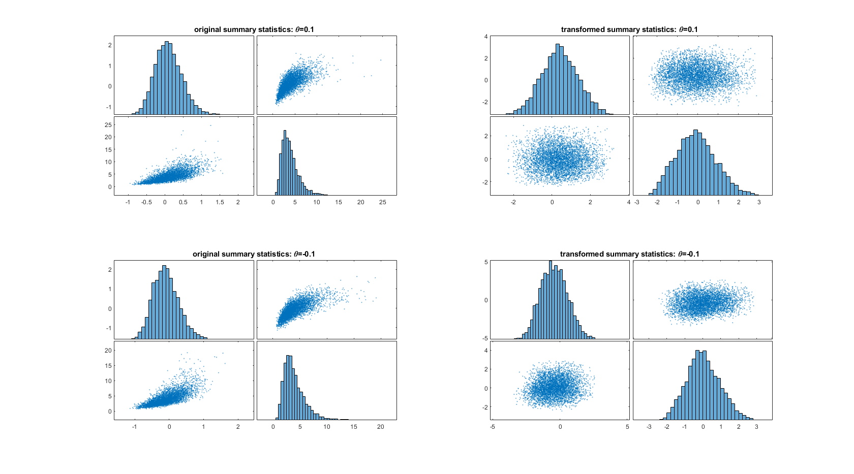
Figure 2: Toy example: The left panels show the scatter plots of the original summary statistics generated at two $\theta$ values, $-0.1$ and $0.1$, different from $\theta_{0}$. The right panels show the scatter plots of the transformed summary statistics, using the WG transformation $T(\theta_{0})$ trained using data generated at $\theta_{0}$.

To examine if these summary statistics follow a normal distribution, we generate $M=5000$ datasets, each of size $n=30$, from (18) with $\theta=0$. The scatter plots in the left panel of Figure 1 indicate that the summary statistics do not follow a normal distribution. Dividing these datasets into a training, validation and test set, we now run Algorithm 3 for training a WG transformation $T$. The right panel of Figure 1 shows the lower bound on the validation set; its middle panel shows the scatter plots of the transformed summary statistics, which indicates that they follow a normal distribution.

The WG transformation $T$ was trained using simulated datasets generated from the model with $\theta=\theta_{0}=0$, i.e. $T=T(\theta_{0})$. To test the robustness of this transformation at different $\theta$, we generate two batches of datasets, one at $\theta=-0.1$ and the other at $\theta=0.1$. Figure 2 shows the scatter plots of the original summary statistics and the transformed statistics using the transformation $T(\theta_{0})$. The plots indicate that the transformed statistics still approximately follow a normal distribution.

We now run two BSL procedures for Bayesian inference about $\theta$ based on the observed data $y_{\text{obs}}$. The first BSL procedure uses MCMC to approximate the posterior in (3), with the sample mean $\widehat{\mu}(\theta)$ and covariance $\widehat{\Sigma}(\theta)$ in (20) calculated based on the summary statistics $s_{i}$. The second BSL procedure also uses MCMC to approximate the posterior in (3), but it uses the transformed statistics $\widetilde{s}_{i}=T(s_{i})$ to calculate $\widehat{\mu}(\theta)$ and $\widehat{\Sigma}(\theta)$. We will refer to the second BSL method as BSL with Wasserstein Gaussianization (BSL-WG). All the settings of these two MCMC schemes are the same; Figure 3 show the trace plots. As shown, it is very challenging for the Markov chain from the standard BSL to converge, while the chain from BSL-WG is mixing well and concentrates around the true parameter $\theta=0$.

Figure 3: Toy example: trace plots of Markov chains from the conventional BSL method and the BSL-WG method.

3.4 Robust BSL with Wasserstein Gaussianization

As robust BSL still requires the normality assumption, it is natural to combine the WG method described in the previous section with robust BSL. We refer to this method as rBSL-WG. Let $T$ be the WG transformation trained at some central value $\theta_{0}$. The rBSL-WG works with the following posterior

$$\overline{\pi}_{\text{rBSL-WG}}(\theta,\Gamma)\propto p(\theta)p(\Gamma)\overline{p}_{\text{rBSL-WG}}(s_{\text{obs}}|\theta,\Gamma),$$ (19)

where

$$\overline{p}_{\text{rBSL-WG}}(s_{\text{obs}}|\theta,\Gamma)=\int N_{d}\big{(}s_{\text{obs}};\widetilde{\mu}_{\text{WG}}(\theta,\Gamma),\widehat{\Sigma}_{\text{WG}}(\theta)\big{)}dy_{1}...dy_{N}.$$

Here,

$$\widehat{\mu}_{\text{WG}}(\theta)=\frac{1}{N}\sum_{j=1}^{N}T(s_{j}),\;\;\;\widehat{\Sigma}_{\text{WG}}(\theta)=\frac{1}{N}\sum_{j=1}^{N}(T(s_{j})-\hat{\mu}_{\text{WG}}(\theta))(T(s_{j})-\hat{\mu}_{\text{WG}}(\theta))^{\top},$$ (20)

and

$$\widetilde{\mu}_{\text{WG}}(\theta,\Gamma)=\widehat{\mu}(\theta)+\text{\rm diag}(\widehat{\Sigma}_{\text{WG}}(\theta))^{1/2}\circ\Gamma.$$

Our VB algorithm for rBSL-WG is the same as Algorithm 2, except that the sample mean and sample covariance in (11) are replaced by

$$\widehat{\mu}_{\text{WG}}(\theta_{i})=\frac{1}{N}\sum_{j=1}^{N}T\big{(}s_{j}^{(i)}\big{)},\;\;\;\widehat{\Sigma}_{\text{WG}}(\theta_{i})=\frac{1}{N}\sum_{j=1}^{N}\big{(}T(s_{j}^{(i)})-\hat{\mu}_{\text{WG}}(\theta_{i})\big{)}\big{(}T(s_{j}^{(i)})-\hat{\mu}_{\text{WG}}(\theta_{i})\big{)}^{\top}.$$

4 Numerical examples and applications

This section implements and compares the performance of the four BSL methods using VB for inference: standard BSL (VB-BSL), robust BSL (VB-rBSL), standard BSL with Wasserstein Gaussianization (VB-BSL-WG) and robust BSL with Wasserstein Gaussianization (VB-rBSL-WG). The implementation was in Python and run on a Dell computer equipped with an Intel Core i7-1265U 1.80 GHz processor and 10 CPU cores. The computer code for the examples is available at https://github.com/VBayesLab/VBSL-WG.

4.1 Toy example

We consider again the toy example outlined in Section 3.3. For each iteration in the VB Algorithm 2, we generate $S=400$ samples of $\theta$, from each of which we simulate $N=200$ datasets each of size $n=200$. The algorithmic parameters for Wasserstein Gaussianization transformation $T$ are as in Section 3.3.

(a) VB-BSL

(b) VB-rBSL

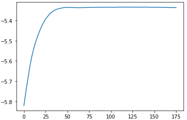
(c) VB-BSL-WG

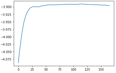
(d) VB-rBSL-WG

Figure 4: Toy example: The smoothed lower bounds for the four VB algorithms.

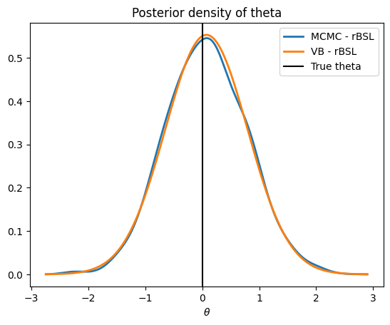
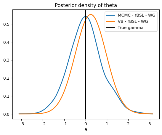
Figure 5: Toy example: VB v.s. MCMC.

We first compare VB with MCMC as the estimation methods for the rBSL and rBSL-WG. Figure 5 plots the posterior estimates of $\theta$, which show that VB and MCMC estimates are almost identical. Interestingly, the rBSL method is able to recover the true model parameter in this example, although there is no model misspecification. This suggests that the rBSL helps robustify and accommodate the normality assumption to some extent; see Frazier and Drovandi, (2021) for more detailed discussion.

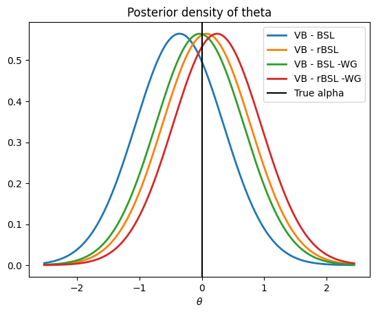
Figure 6: Toy example: The plot shows variational posterior across the four BSL methodologies.

We now compare the different Bayesian synthetic likelihood methods using VB and MCMC for estimation. Figure 4 plots the smoothed lower bound of the four VB algorithms, which indicates that all the four algorithms have converged. We note that it is not meaningful to compare the magnitude of these lower bounds as they come from different models and parameterization. Figure 6 shows the plot of the VB posterior estimates. Table 1 shows the mean squared error (MSE) between the posterior mean estimate of $\theta$ and the true $\theta$, across 10 different runs. The results show that adding the Wasserstein Gaussianization into the BSL method is useful and helps improve the estimation accuracy. There is a substantial improvement of the rBSL and rBSL-WG over the standard BSL. The VB-rBSL-WG is slightly better than VB-rBSL. This might be because of the oversimplicity in this one-dimensional example; we observe bigger improvement in the more sophisticated examples in the next sessions.

	VB-BSL	VB-rBSL	MCMC-rBSL	VB-BSL-WG	VB-rBSL-WG	MCMC-rBSL-WG
$||\theta_{true}-\hat{\theta}||_{2}$	0.0509 (0.0236)	0.0129 (0.0069)	0.0065 (0.0042)	0.0123 (0.0109)	0.0092 (0.0054)	0.0002 (0.0001)

Table 1: Toy example: The avaraged MSE, over the replicates, of the parameter estimates across the six BSL methods. The numbers in brackets are standard deviations.

4.2 $\alpha$-stable model example

This section applies the BSL methods to Bayesian inference in the $\alpha$-stable model (Nolan,, 2007), which is a family of heavy-tailed distributions that have seen applications in situations with rare but extreme events. This family of distributions poses challenges for inference because there exists no closed form expression for the density function. The $\alpha$-stable distribution is often defined using its log characteristic function (Samorodnitsky and Taqqu,, 2017)

$$\log\phi(t)=\begin{cases}-\gamma^{\alpha}|t|^{\alpha}{1-i\beta\text{sign}(t)\tan\frac{\pi\alpha}{2}}+i\delta t,&\alpha\neq 1\\ -\gamma|t|{1+i\beta\text{sign}(t)\frac{2}{\pi}\log|t|}+i\delta t,&\alpha=1,\end{cases}$$

where $\theta=(\alpha,\beta,\gamma,\delta)$ are the model parameters and $\text{sign}(t)$ is equal to 1 if $t\geq 0$ and -1 if $t<0$. As for the observed data, we simulated a dataset of size $n=200$ with the true parameters $(\alpha,\beta,\gamma,\delta)=(1.8,0.5,1,0)$.

We now test the ability of the BSL methods to recover the true parameter together with the estimation uncertainty. We follow Peters et al., (2012) and enforce the constraints $\alpha\in(1.1,2)$, $\beta\in(-1,1)$, $\gamma>0$, and work with the following reparametrization of $\theta$

$$\tilde{\alpha}=\log\frac{\alpha-1.1}{2-\alpha},\quad\tilde{\beta}=\log\frac{\beta+1}{1-\beta},\quad\tilde{\gamma}=\log\gamma,\quad\tilde{\delta}=\delta.$$

We use a normal prior $N(0,100I_{4})$ for $\tilde{\theta}$ as in Tran et al., (2017). We then approximate the posterior of $\tilde{\theta}=(\tilde{\alpha},\tilde{\beta},\tilde{\gamma},\tilde{\delta})$, but the results below will be reported in terms of the original parameter $\theta$.

For the Wasserstein Gaussianization, we first run the standard VB-BSL algorithm to get an estimate, $\theta_{0}$, of the posterior mean of $\theta$. We then simulate 3000 datasets, each of size 50, from the $\alpha$-stable distribution at $\theta_{0}$ and calculate the summary statistics. For the four summary statistics used in the $\alpha$-stable distribution, we refer the interested readers to Peters et al., (2012). We divide the 3000 sets of summary statistics into three sets, each of 1000, for training, validation and testing. The left panel in Figure 7 shows a scatter plot among the summary statistics which clearly indicates that the summary statistics do not follow a normal distribution. The middle panel in Figure 7 shows the scatter plot of the WG transformed summary statistics on the test dataset, which is much closer to the scatter plot of a normal distribution. The right panel shows the lower bound from Algorithm 3. The training time for WG was 2.8 minutes.

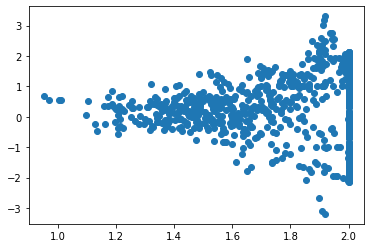
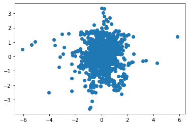
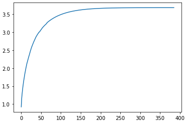
Figure 7: $\alpha$-stable model: The scatter plots of the original and WG transformed summary statistics. The right plot shows the lower bound (17) on the validation set.

We first compare VB with MCMC as the estimation methods. Figures 8 and 9 plot the posterior estimates, obtained by VB and MCMC, for the rBSL and rBSL-WG methods, respectively. The results confirm the accuracy of VB, compared to MCMC. In each VB iteration, we generated $S=400$ samples of $\theta$, from each of which we simulated $N=200$ datasets each of size $n=200$ from the $\alpha$-stable distribution. The MCMC procedure was run for 20,000 iterations. The CPU times for MCMC-rBSL and MCMC-rBSL-WG were 133.3 minutes and 141.5 minutes, respectively. The VB methods were faster, with the CPU times of 23.3 minutes and 42.8 minutes for VB-rBSL and VB-rBSL-WG, respectively. These times do not include the training time for WG. Each iteration in the VB methods was run in parallel across the $\theta$-samples, therefore we could reduce the computation time further if more CPU cores were available.

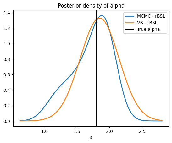
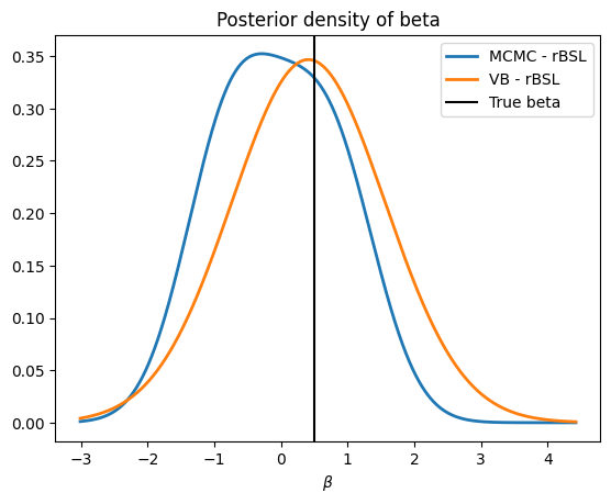
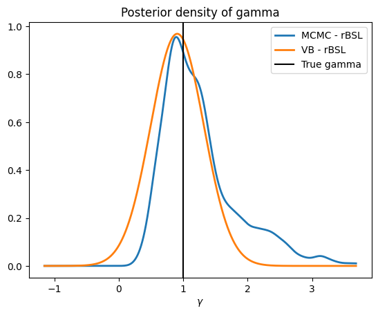
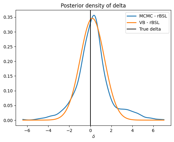
Figure 8: $\alpha$-stable model: VB and MCMC posterior estimates for rBSL.

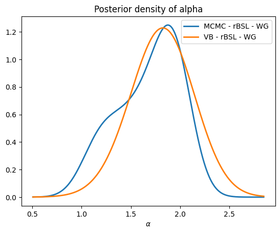
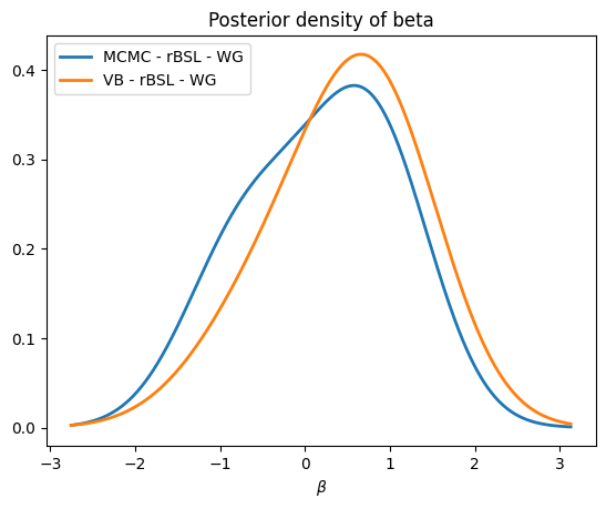
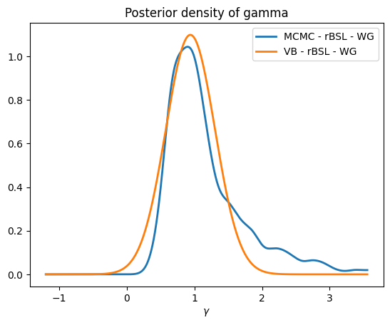
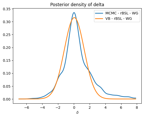
Figure 9: $\alpha$-stable model: VB and MCMC posterior estimates for rBSL-WG.

We now run the four BSL methods with VB as the estimation method: standard BSL, rBSL, BSL-WG and rBSL-WG. We aim to test the ability of these BSL methods in terms of recovering the true model parameters. Figure 10 plots the variational distribution of the four parameters $\alpha$, $\beta$, $\gamma$, $\delta$. The VB-BSL performs the worst with the estimates for $\alpha$, $\beta$ and $\delta$ far from the true values. To have a better measure of the performance of the methods, we repeat this example ten times and compute the average MSE and Mahalanobis distance between the posterior mean estimates and the true parameters. The Mahalanobis distance is calculated as

$$\text{MD}(||\theta_{true}-\hat{\theta}||)=\sqrt{(\theta_{true}-\hat{\theta}){\hat{\Sigma}}^{-1}(\theta_{true}-\hat{\theta})^{\top}}$$

where $\hat{\theta}$ and $\hat{\Sigma}$ are the mean and covariance matrix obtained from the optimal variational Gaussian distribution. The MSE, Mahalanobis distance values and CPU times are summarized in Table 2. As observed from the table, the VB-rBSL-WG method produces the most accurate estimate, followed by VB-BSL-WG. Incorporating the WG transformation into BSL leads to a significant improvement in terms of recovering the true model parameters.

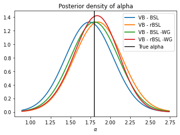
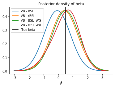
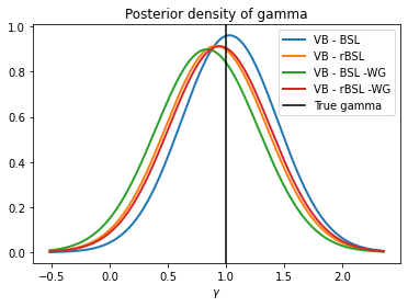
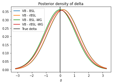
Figure 10: $\alpha$-stable model: Marginal variational posterior distributions for the four parameters ($\alpha$, $\beta$, $\gamma$, $\delta$) across the four BSL methods (better viewed in colour).

	VB-BSL	VB-rBSL	VB-BSL-WG	VB-rBSL-WG
$||\theta_{\text{true}}-\hat{\theta}||_{2}$	0.3182 (0.009)	0.2367 (0.003)	0.0918 (0.005)	0.0834 (0.004)
MD$(||\theta_{true}-\hat{\theta}||)$	3.1967 (0.0359)	2.4116 (0.0204)	0.9594 (0.0108)	0.7371 (0.0252)
CPU time	9.1	23.3	41.0	42.8

Table 2: $\alpha$-stable model: MSE and Mahalanobis distance of the posterior mean estimates compared to $\theta_{\text{true}}$, over 10 different runs, and the CPU times (in minutes per run) across the four BSL methods. The numbers in brackets are standard deviations.

4.3 g-and-k example

The g-and-k distributions are a family of flexible distributions often used to model highly skewed data. These distributions are defined through their quantile function (Rayner and MacGillivray,, 2002), hence their density function is not available in closed form, but it is easy to generate data from them. Estimating a g-and-k distribution has been a common example in the literature to test the performance of likelihood-free inference methods (Drovandi and Pettitt,, 2011).

The quantile function $Q(p)$, $p\in(0,1)$, of the g-and-k distribution is given as follows

$$Q(p)=A+B\Bigr{[}1+0.8\frac{1-e^{-gz(p)}}{1+e^{-gz(p)}}\Bigr{]}\big{(}1+z(p)^{2}\big{)}^{k}z(p),$$ (21)

where $z(p)$ is the quantile function of the standard normal distribution. This model has four parameters, $A$, $B$, $g$ and $k$. It is straightforward to generate a sample $X$ from this model using $X=Q(U)$ with $U\sim U[0,1]$. We generated an observed dataset of size 200 with the true parameters $\theta_{\text{true}}=(A,B,g,k)=(3,1,2,0.5)$.

For the summary statistics, we follow Drovandi and Pettitt, (2011) and use

$$s_{A}=O_{4},\quad s_{B}=O_{6}-O_{2},\quad s_{g}=\frac{O_{7}-O_{5}+O_{3}-O_{1}}{s_{B}},\quad s_{k}=\frac{O_{6}+O_{2}-2O_{4}}{s_{B}},$$

where $O_{j}$ is the $j$-th octile of the data. The left panel in Figure 11 shows the scatter plots of these four summary statistics, based on 500 datasets, each of size 200, generated from the g-and-k distribution at $\theta_{\text{true}}$. It can be seen that these summary statistics are far from a multivariate normal distribution. For example, the scatter plot of $s_{B}$ and $s_{k}$ is far from an elliptic. The right panel shows the scatter plots of the transformed summary statistics.

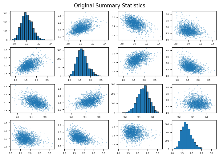
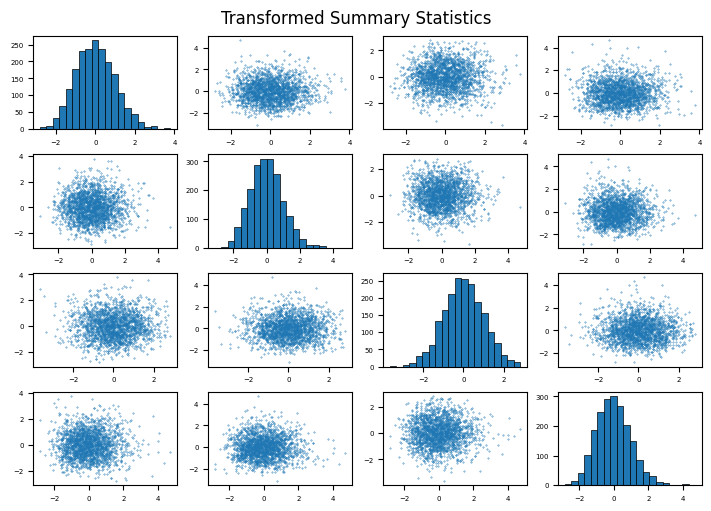
Figure 11: g-and-k model: The left panel shows the original summary statistics. The right panel shows their WG transformations.

Figure 12 plots the variational distributions of the four parameters $A$, $B$, $g$, $k$. It shows that the VB-rBSL-WG method, compared to the other three methods, locates its estimates closer to the true model parameters. Table 3 summarizes the average MSE and Mahalanobis distance values, across 10 different runs, between the posterior mean estimates and the true model parameters. The results confirm the superior performance of the VB-rBSL-WG method, followed by the VB-BSL-WG in terms of the MSE and by the VB-rBSL in terms of the Mahalanobis distance.

	VB-BSL	VB-rBSL	VB-BSL-WG	VB-rBSL-WG
$||\theta_{\text{true}}-\hat{\theta}||_{2}$	0.6873 (0.0019)	0.6671 (0.0017)	0.5020 (0.0081)	0.2159 (0.0023)
MD$(||\theta_{true}-\hat{\theta}||)$	6.8771 (0.1967)	6.6267 (0.005)	8.5730 (0.0291)	5.4587 (0.0048)
CPU time	63.9	199.5	801.9	937.6

Table 3: g-and-k example: MSE and Mahalanobis distance of the posterior mean estimates compared to $\theta_{\text{true}}$, over 10 different runs, and the CPU times (in minutes per run) across the four BSL methods. The numbers in brackets are standard deviations.

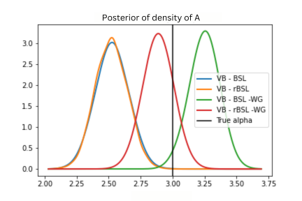
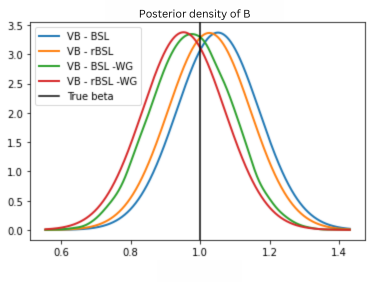
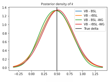
Figure 12: g-and-k model. Marginal variational posterior distributions for the four parameters ($A$, $B$, $g$, $k$) across the four BSL methods (better viewed in colour).

4.4 Fowler’s toads example

The study of movement patterns in amphibian animals is a topic of great interest in ecology. To investigate these patterns, Marchand et al., (2017) developed a stochastic movement model based on their research of Fowler’s toads at Long Point in Ontario, Canada. The model assumes that the toads hide in a refuge site during the day and forage during the night, which is a common behavior for these animals, and that every toad goes through two sequential processes. First, the overnight displacement $\Delta y$ follows a Levy-alpha stable distribution $S(\alpha,\gamma)$. Second, the toad’s return behavior is modelled by a probability model with $p_{0}$ the probability that the toad selects at random one of the previous refuge sites. More details about the model can be found in Marchand et al., (2017).

The radio-tracking device collects the information of $n_{t}$ toads on $n_{d}$ days to create an observation matrix $\mathbb{Y}$ of dimension $n_{d}\times n_{t}$. The actual data has a dimension of $(n_{d}=63)\times(n_{t}=66)$. For ease of comparison, we use a simulated data in this paper, where the observed data of size $(n_{d}=63)\times(n_{t}=66)$ were generated from the model at the true parameter $\theta_{\text{true}}=(\alpha,\gamma,p_{0})=(1.7,35,0.6)$.

For the summary statistics, we follow Marchand et al., (2017) and summarize the data $\mathbb{Y}$ into four sets $\mathbb{y}_{1},...,\mathbb{y}_{4}$ of relative moving distances for four different time lags: 1, 2, 4 and 8 days. For example, $\mathbb{y}_{2}$ represents the displacement information within a lag of 2 days: $\mathbb{y}_{2}=\{|\mathbb{Y}_{i,j}-\mathbb{Y}_{i+2,j}|;1\leq i\leq n_{d}-2,1\leq j\leq n_{t}\}$. Within each set $\mathbb{y}_{j}$, we split the displacements into two subsets. The first subset consists of the displacements with absolute values less than 10 meters, in which cases the toad is considered as having returned to its original location. The number of such returns is used as the first summary statistics. For the second subset consisting of displacements with absolute values larger than 10 meters (non-returns), we calculate the log difference between the min, median and max, leading to two summary statistics. Putting together, we obtain the summary statistics of size 3 for each lag, and hence summarizing the entire data down to 12 ($=3\times 4$ lags) statistics. We note that the previous literature used the log difference between eleven quantiles 0, 10th,…,100th; leading to 48 summary statistics in total. We opt to reduce the size of the summary statistics for computational purposes.

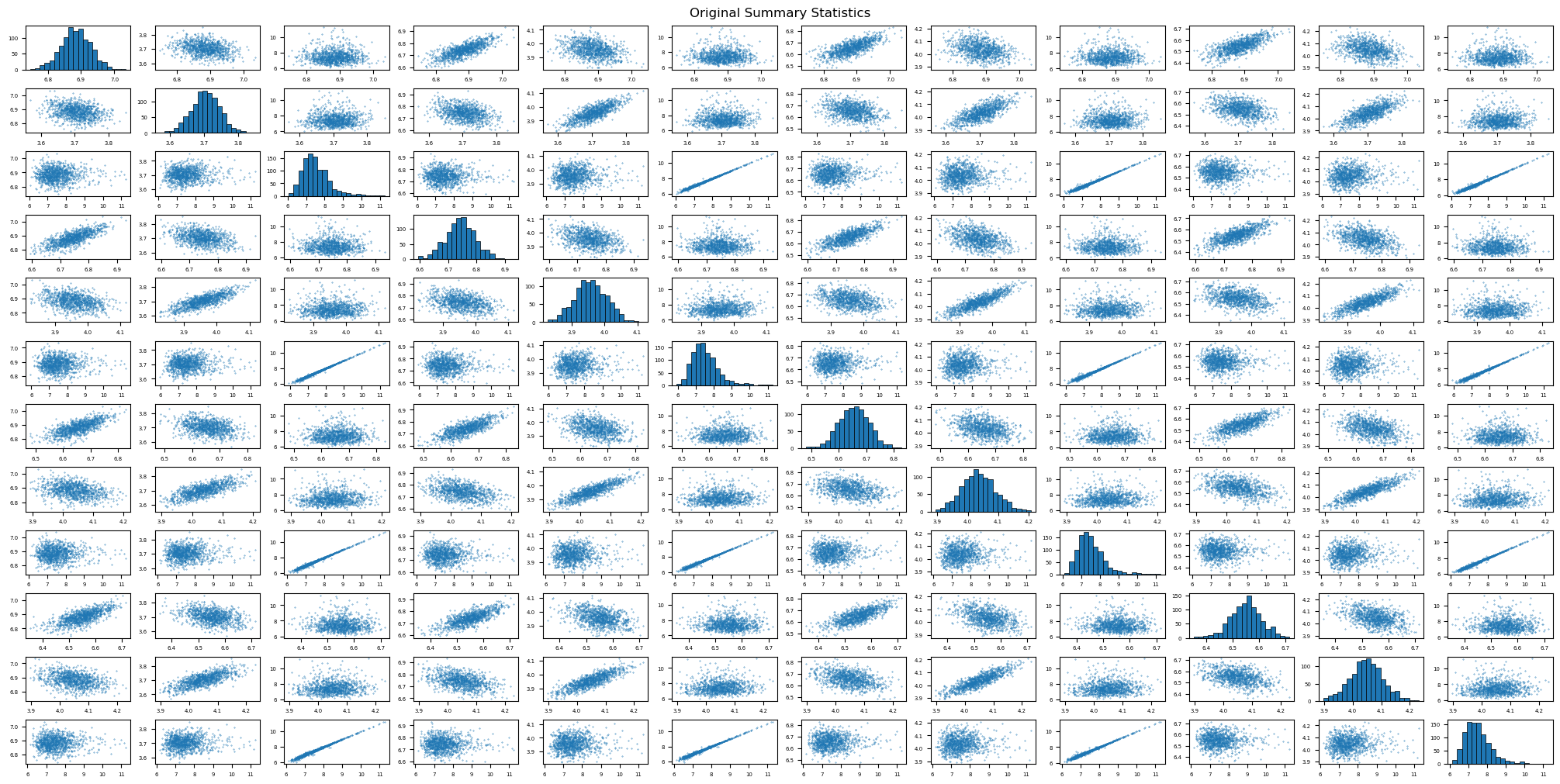
Figure 13: Toads’ movement model: scatter plots of the original summary statistics.

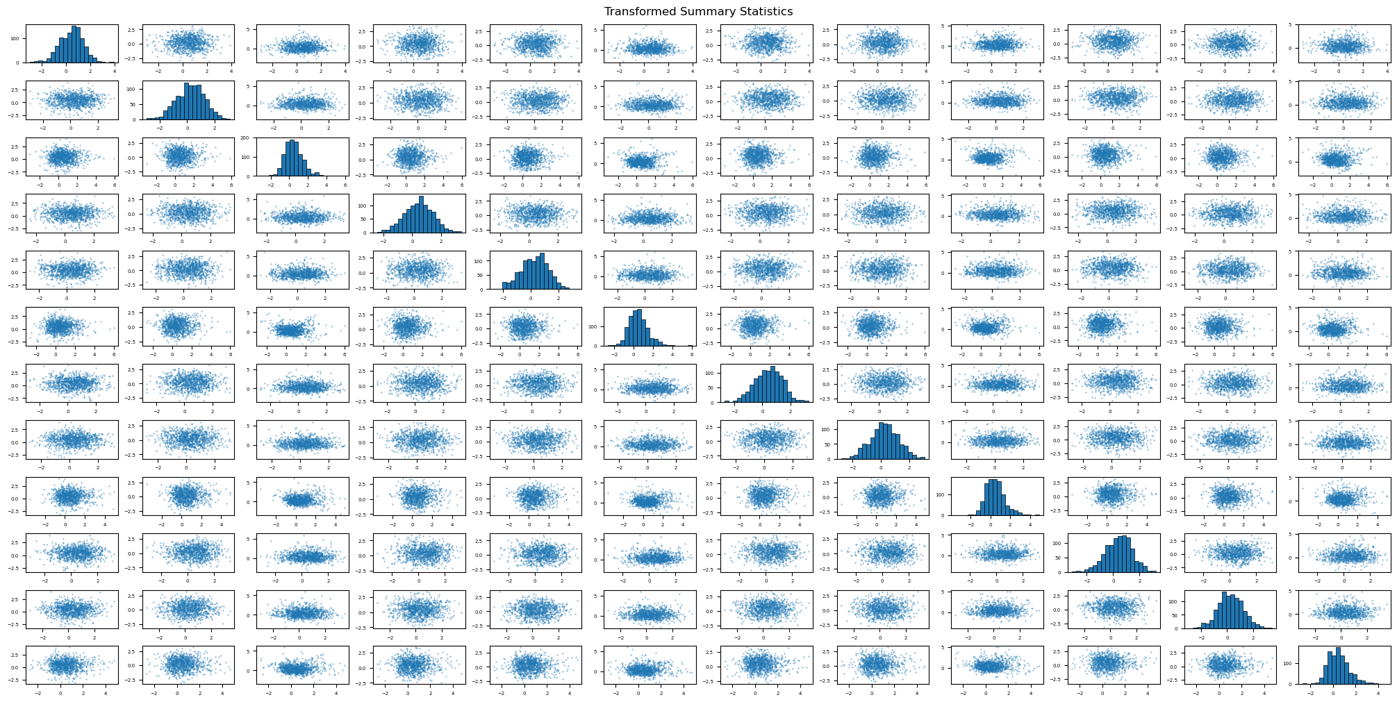
Figure 14: Toads’ movement model: scatter plots of the WG transformed summary statistics.

Figure 13 shows that the summary statistics do not follow a multivariate normal distribution. The transformed summary statistics using the WG transformation is shown in Figure 14. Table 4 reports the average MSE values and Mahalanobis distance, over 10 different runs, between the posterior mean estimates and the true parameters. The results indicate that the rBSL-WG method helps reduce significantly the estimation bias.

	VB-BSL	VB-rBSL	VB-BSL-WG	VB-rBSL-WG
$||\theta-\hat{\theta}||_{2}$	3.1772 (0.0218)	2.6773 (0.0185)	2.9632 (0.0291)	0.6526 (0.0161)
MD$(||\theta_{true}-\hat{\theta}||)$	30.8722 (0.3153)	27.0151 (0.1869)	32.4161 (0.3181)	14.4733 (0.2585)
CPU time	1250	1361	1410	1532

Table 4: Toads’ movement example: MSE and Mahalanobis distance of the posterior mean estimates compared to $\theta_{\text{true}}$, over 10 different runs, and the CPU times (in minutes per run) across the four BSL methods. The numbers in brackets are standard deviations.

5 Conclusion

Our WG transformation combined with rBSL and efficient VB provides a powerful and flexible approach to inference in likelihood-free problems that overcomes many of the limitations of existing methods. We hope that this paper will encourage the wider adoption of likelihood-free methods in a range of applications, where they offer an attractive alternative to traditional methods. While our WG transformation has shown promising results, further improvements are possible for its use in high-dimensional settings. One potential avenue for improvement is to incorporate an adaptive learning rate or natural gradient, and research in this direction is currently underway.

References

- Ambrosio et al., (2005) Ambrosio, L., Gigli, N., and Savaré, G. (2005). Gradient Flows In Metric Spaces and in the Space of Probability Measures. Birkhauser.
- An et al., (2020) An, Z., Nott, D. J., and Drovandi, C. (2020). Robust Bayesian synthetic likelihood via a semi-parametric approach. Statistics and Computing, 30(3):543–557.
- Barbu et al., (2018) Barbu, C. M., Sethuraman, K., Billig, E. M., and Levy, M. Z. (2018). Two-scale dispersal estimation for biological invasions via synthetic likelihood. Ecography, 41(4):661–672.
- Blei et al., (2017) Blei, D. M., Kucukelbir, A., and McAuliffe, J. D. (2017). Variational inference: A review for statisticians. Journal of the American Statistical Association, 112(518):859–877.
- Dao et al., (2022) Dao, V.-H., Gunawan, D., Tran, M.-N., Kohn, R., Hawkins, G., and Brown, S. (2022). Efficient selection between hierarchical cognitive models: Cross-validation with Variational Bayes. Psychological Methods. In Press.
- Drovandi and Pettitt, (2011) Drovandi, C. C. and Pettitt, A. N. (2011). Likelihood-free Bayesian estimation of multivariate quantile distributions. Computational Statistics & Data Analysis, 55(9):2541–2556.
- Fasiolo et al., (2016) Fasiolo, M., Pya, N., and Wood, S. N. (2016). A comparison of inferential methods for highly nonlinear state space models in ecology and epidemiology. Statistical Science, pages 96–118.