Optimal Control of Logically Constrained
Partially Observable and Multi-Agent
Markov Decision Processes

Abstract

Autonomous systems often have logical constraints arising, for example, from safety, operational, or regulatory requirements. Such constraints can be expressed using temporal logic specifications. The system state is often partially observable. Moreover, it could encompass a team of multiple agents with a common objective but disparate information structures and constraints. In this paper, we first introduce an optimal control theory for partially observable Markov decision processes (POMDPs) with finite linear temporal logic ($\boldsymbol{\textsc{LTL}_{f}}$) constraints. We provide a structured methodology for synthesizing policies that maximize a cumulative reward while ensuring that the probability of satisfying a temporal logic constraint is sufficiently high. Our approach comes with guarantees on approximate reward optimality and constraint satisfaction. We then build on this approach to design an optimal control framework for logically constrained multi-agent settings with information asymmetry. We illustrate the effectiveness of our approach by implementing it on several case studies.

I Introduction

Autonomous systems are rapidly being deployed in many safety-critical applications like robotics, transportation, and advanced manufacturing. Markov decision processes (MDPs) [1] can model a wide range of sequential decision-making scenarios in these dynamically evolving environments. Traditionally, a reward structure is defined over the MDP state-action space, and is then maximized to achieve a desired objective. Formulating an appropriate reward function is critical, as an incorrect formulation can easily lead to unsafe and unforeseen behaviors. Designing reward functions for complex specifications can be exceedingly difficult and may not always be possible.

Increasing interest has been directed over the past decade toward leveraging tools from formal methods and temporal logic [2] to alleviate this difficulty. These tools allow unambiguously specifying, solving, and validating complex control and planning problems. Temporal logic formalisms are capable of capturing a wide range of task specifications, including surveillance, reachability, safety, and sequentiality. However, while certain objectives like safety or reachability are well expressed by temporal logic constraints, others, e.g., pertaining to system performance or cost, are often better framed as “soft” rewards to be maximized. In this paper, we focus on such composite tasks.

While full state observability is assumed in environments modeled by MDPs, this assumption excludes many real-life scenarios where the state is only partially observed. These scenarios can instead be captured by partially observable Markov decision processes (POMDPs). In theory, any POMDP can be translated into an equivalent MDP in which the MDP state is the posterior belief on the POMDP state [3]. However, due to the exponentially growing state-space in this approach, planning methods developed for MDPs become intractable in practice. The same difficulty holds when applying methods developed for synthesizing MDP policies that satisfy temporal logic specifications in the context of POMDPs. In this paper, we expand the traditional POMDP framework to incorporate temporal logic specifications. Specifically, we aim to synthesize policies such that the agent’s cumulative reward is maximized while the probability of satisfying a given temporal logic specification is above a desired threshold.

We consider finite linear temporal logic ($\textsc{LTL}_{f}$) [4], a temporal extension of propositional logic, to express complex tasks. $\textsc{LTL}_{f}$ is a variant of linear temporal logic (LTL) [2], which is interpreted over finite length strings rather than infinite length strings. For a given $\textsc{LTL}_{f}$ specification, we can construct a deterministic finite automaton (DFA) such that the agent’s trajectory satisfies the specification if and only if it is accepted by the DFA [5]. Therefore, augmenting the system state with the DFA’s internal state enables us to keep track of both the environment as well as the task status.

We can then reason about the cumulative POMDP reward and the temporal logic satisfaction simultaneously by formulating the planning problem as a constrained POMDP problem. We address the constrained POMDP problem by proposing an iterative scheme which solves a sequence of unconstrained POMDP problems using any off-the-shelf unconstrained POMDP solver [6, 7], thus leveraging existing results from unconstrained POMDP planning.

Finally, we extend our framework to a multi-agent setting with information asymmetry. We use the previously described approach for composition with the DFA to obtain a constrained multi-agent planning problem and similarly reduce this problem to multiple unconstrained multi-agent problems. Under some mild assumptions, these unconstrained multi-agent problems can be viewed as single-agent POMDP problems via the common information approach [8]. Owing to the theoretical guarantees of the common information approach and our algorithm, the returned policies will still provide the desired guarantees on optimality and temporal logic satisfaction.

Our contributions can be summarized as follows: (i) We formulate a novel optimal control problem in terms of cumulative reward maximization in POMDPs under expressive $\textsc{LTL}_{f}$ constraints. (ii) We design an iterative planning scheme which can leverage any off-the-shelf unconstrained POMDP solver to solve the problem. Differently from existing work on constrained POMDPs, our scheme uses a no-regret online learning approach to provide theoretical guarantees on the near-optimality of the returned policy. (iii) We extend the single-agent framework to a multi-agent setting with information asymmetry, where agents have a common reward objective but can have individual or even joint temporal logic requirements. Their different information structure makes the problem rather difficult. (iv) We conduct experimental studies on a suite of single and multi-agent environments to validate the algorithms developed and explore their effectiveness. To the best of our knowledge, this is the first effort on optimal control of logically constrained partially observed and multi-agent MDP models.

We presented some preliminary results on optimal control of POMDPs with $\textsc{LTL}_{f}$ specifications in a previous publication [9]. In this paper, we consider POMDPs with both $\textsc{LTL}_{f}$ specifications and reward constraints, we discuss the extension to the multi-agent setting with information asymmetry, and introduce practical algorithms that can use approximate POMDP solvers. Furthermore, we include the proofs of all the theorems.

II Related Work

Synthesizing policies for MDPs such that they maximize the probability of satisfying a temporal logic specification has been extensively studied in the context of known [10, 11] and unknown [12, 13] transition probabilities.

Several approaches have also been proposed for maximizing the temporal logic satisfaction probability in POMDPs, albeit without considering an additional reward objective. Some of these methods include building a finite-state abstraction via approximate stochastic simulation over the belief space [14], grid-based discretization of the POMDP belief space [15], and restricting the space of policies to finite state controllers [16, 17]. Similarly to our work, leveraging well-studied unconstrained POMDP planners [18, 19] has also been proposed in this context, while deep learning approaches like those using recurrent neural networks [20, 21] have been lately explored.

Our approach further differs from a few other existing methods for solving constrained POMDPs. One of these methods [22] iteratively constructs linear programs which result in an approximate solution for the constrained POMDP problem. Another method addresses the scalability issues of the previous one using a primal-dual approach based on Monte Carlo Tree Search (MCTS) [23]. We solve the constrained POMDP problem using a similar method. A key difference is that, instead of using an MCTS approach, we use an approximate unconstrained POMDP solver, SARSOP [6], which returns policies along with bounds on their optimality gaps. Column generation algorithms [24] also use a primal-dual approach, but with a different dual parameter update procedure. While only convergence to optimality is discussed for these algorithms, our method, on the other hand, gives a precise relationship between the approximation error and the number of iterations.

A few methods have also appeared which address temporal logic satisfaction in a multi-agent setting, albeit leveraging different formulations and solution strategies. Some examples include the synthesis of a joint policy maximizing the temporal logic satisfaction probability for multiple agents with shared state space [25] and the decomposition of temporal logic specifications for scalable planning for a large number of agents under communication constraints [26, 27]. Some efforts have also leveraged the robustness semantics of temporal logics to guide reward shaping for multi-agent planning [28, 29]. To the best of our knowledge, our method is the first to consider a reward objective and a temporal logic constraint in the multi-agent stochastic setting with information asymmetry.

III Preliminaries

We denote the sets of real and natural numbers by $\mathbb{R}$ and $\mathbb{N}$, respectively. $\mathbb{R}_{\geq 0}$ is the set of non-negative reals. For a given finite set $S$, $S^{*}$ denotes the set of all finite sequences of elements taken from $S$. We use $A^{1:n}$ as a shorthand for $(A^{1},\ldots,A^{n})$ and $A_{1:n}$ as a shorthand for $(A_{1},\ldots,A_{n})$. The indicator function $\mathds{1}_{S}(s)$ evaluates to $1$ when $s\in S$ and 0 otherwise. For a singleton set $\{s_{0}\}$, we will denote $\mathds{1}_{\{s_{0}\}}(s)$ by $\mathds{1}_{s_{0}}(s)$ for simplicity. The probability simplex over the set $S$ is denoted by $\Delta_{S}$. For a string $s$, $|s|$ denotes its length.

III-A Labeled POMDPs

III-A1 Model

A Labeled Partially Observable Markov Decision Process is defined as a tuple $\mathscr{M}=({\mathcal{S}},{{\mathcal{U}}},P,\varpi,{O},Z,AP,L,r^{o},r^{c},T)$, where ${\mathcal{S}}$ is a finite state space, ${{\mathcal{U}}}$ is a finite action space, $P_{t}(s,u;s^{\prime})$ is the probability of transitioning from state $s$ to state $s^{\prime}$ on taking action $u$ at time $t$, $\varpi\in\Delta_{\mathcal{S}}$ is the initial state distribution, ${O}$ is a finite observation space, $Z_{t}(s;o)$ is the probability of seeing observation $o$ in state $s$ at time $t$, $AP$ is a set of atomic propositions, used to indicate the truth value of a predicate (property) of the state, e.g., the presence of an obstacle or goal state. $L:{\mathcal{S}}\to 2^{AP}$ is a labeling function which indicates the set of atomic propositions which are true in each state, e.g., $L(s)=\{a\}$ indicates that only the atomic proposition $a$ is true in state $s$. $r^{o}_{t}(s,u)$ and $r^{c}_{t}(s,u)$ are the objective and constraint rewards obtained on taking action $u$ in state $s$ at time $t$. The state, action, and observation at time $t$ are denoted by $\mathcal{S}_{t}$, ${\mathcal{U}}_{t}$, and $O_{t}$, respectively. At any given time $t$, the information available to the agent is the collection of all the observations $O_{0:t}$ and all the past actions ${\mathcal{U}}_{0:t-1}$. We denote this information with $I_{t}=\{O_{0:t},{\mathcal{U}}_{0:t-1}\}$. We say that the system is time-invariant when the reward functions $r^{o}_{t},r^{c}_{t}$ and the transition and observation probability functions $P_{t}$ and $Z_{t}$ do not depend on time $t$. The POMDP runs for a random time horizon $T$. This random time may be determined exogenously (independently) of the POMDP or it may be a stopping time with respect to the information process $\{I_{t}:t\geq 0\}$.

III-A2 Pure and Mixed Policies

A control law $\pi_{t}$ maps the information $I_{t}$ to an action in the action space ${\mathcal{U}}$. A policy $\pi:=(\pi_{0},\pi_{1},\ldots)$ is then the sequence of laws over the entire horizon. We refer to such deterministic policies as pure policies and denote the set of all pure policies with $\mathcal{P}$.

A mixed policy $\mu$ is a distribution on a finite collection of pure policies. Under a mixed policy $\mu$, the agent randomly selects a pure policy $\pi\in\mathcal{P}$ with probability $\mu(\pi)$ before the POMDP begins. The agent uses this randomly selected policy to select its actions during the course of the process. More formally, $\mu:\mathcal{P}\to[0,1]$ is a mapping. The support of the mixture $\mu$ is defined as

$$\mathrm{supp}(\mu):=\{\pi\in\mathcal{P}:\mu(\pi)\neq 0\}.$$ (1)

If the support size of a mixed policy is $1$, then it is a pure policy. The set $\mathcal{M}_{p}$ of all mixed mappings is given by

$$\mathcal{M}_{p}:=\left\{\mu:|\mathrm{supp}(\mu)|<\infty,\sum_{\pi\in\mathrm{supp}(\mu)}\mu(\pi)=1\right\}.$$ (2)

Clearly, the set $\mathcal{M}_{p}$ of mixed policies is convex.

A run ${\xi}$ of the POMDP is the sequence of states and actions $((\mathcal{S}_{0},{\mathcal{U}}_{0}),(\mathcal{S}_{1},{\mathcal{U}}_{1}),\cdots,(\mathcal{S}_{T},{\mathcal{U}}_{T}))$ up to horizon $T$. The total expected objective reward for a policy $\mu$ is given by

$$\mathcal{R}^{\mathscr{M}}_{o}(\mu) ={\mathbb{E}}_{\mu}^{\mathscr{M}}\left[\sum_{t=0}^{T}r^{o}_{t}(\mathcal{S}_{t},{\mathcal{U}}_{t})\right]$$ (3)

$$=\sum_{\pi\in\mathrm{supp}(\mu)}\left[\mu(\pi){\mathbb{E}}_{\pi}^{\mathscr{M}}\left[\sum_{t=0}^{T}r^{o}_{t}(\mathcal{S}_{t},{\mathcal{U}}_{t})\right]\right].$$ (4)

The total expected constraint reward $\mathcal{R}^{\mathscr{M}}_{c}(\mu)$ is similarly defined with respect to $r^{c}$. $\mathcal{R}^{\mathscr{M}}_{o}(\mu)$ and $\mathcal{R}^{\mathscr{M}}_{c}(\mu)$ are linear functions in $\mu$.

Assumption 1.

The POMDP $\mathscr{M}$ is such that for every pure policy $\pi$, the expected value of the random horizon $T$ is bounded by a finite constant and the total expected constraint reward is also bounded above by a finite constant, i.e.,

$${\mathbb{E}}_{\pi}^{\mathscr{M}}[T]<T_{\textsc{max}}<\infty,$$ (5)

$$0\leq\mathcal{R}^{\mathscr{M}}_{c}(\pi)\leq R_{\textsc{max}}\leavevmode\nobreak\ \leavevmode\nobreak\ \forall\ \pi.$$ (6)

Assumption 1 ensures that $T$ is finite almost surely, i.e., ${\mathbb{P}}_{\mu}^{\mathscr{M}}[T<\infty]=1$ and the total expected constraint reward satisfies $\mathcal{R}^{\mathscr{M}}_{c}(\mu)\leq R_{\textsc{max}}$ for every policy $\mu$.

III-B Finite Linear Temporal Logic

We use $\textsc{LTL}_{f}$ [4], a variant of linear temporal logic (LTL) [2] interpreted over finite strings, to express complex task specifications. Given a set $AP$ of atomic propositions, i.e., Boolean variables that have a unique truth value ($\mathsf{true}$ or $\mathsf{false}$) for a given system state, $\textsc{LTL}_{f}$ formulae are constructed inductively as follows:

$$\varphi:=\mathsf{true}\ |\ a\ |\ \neg\varphi\ |\ \varphi_{1}\wedge\varphi_{2}\ |\ \textbf{X}\varphi\ |\ \varphi_{1}\textbf{U}\varphi_{2},$$

where $a\in AP$, $\varphi$, $\varphi_{1}$, and $\varphi_{2}$ are LTL formulae, $\wedge$ and $\neg$ are the logic conjunction and negation, and U and X are the until and next temporal operators. Additional temporal operators such as eventually (F) and always (G) are derived as $\textbf{F}\varphi:=\mathsf{true}\textbf{U}\varphi$ and $\textbf{G}\varphi:=\neg\textbf{F}\neg\varphi$. For example, $\varphi=\textbf{F}a\wedge(\textbf{G}\neg b)$ expresses the specification that a state where atomic proposition $a$ holds true has to be eventually reached by the end of the trajectory and states where atomic proposition $b$ holds true have to be always avoided.

$\textsc{LTL}_{f}$ formulae are interpreted over finite-length words $w=w_{0}w_{1}\cdots w_{last}\in{(2^{AP})}^{*}$, where each letter $w_{i}$ is a set of atomic propositions and $last=|w|-1$ is the index of the last letter of the word $w$. Given a finite word $w$ and $\textsc{LTL}_{f}$ formula $\varphi$, we inductively define when $\varphi$ is $\mathsf{true}$ for $w$ at step $i$, $0\leq i<|w|$, written $(w,i)\models\varphi$. Informally, $a$ is $\mathsf{true}$ for $(w,i)$ iff $a\in w_{i}$; $\textbf{X}\varphi$ is $\mathsf{true}$ for $(w,i)$ iff $\varphi$ is $\mathsf{true}$ for $(w,i+1)$; $\varphi_{1}\textbf{U}\varphi_{2}$ is $\mathsf{true}$ for $(w,i)$ iff there exits $k\geq i$ such that $\varphi_{2}$ is $\mathsf{true}$ for $(w,k)$ and $\varphi_{1}$ is $\mathsf{true}$ for all $j,\ i\leq j<k$; $\textbf{G}\varphi$ is $\mathsf{true}$ for $(w,i)$ iff $\varphi$ is $\mathsf{true}$ for all $(w,j),j\geq i$; $\textbf{F}\varphi$ is $\mathsf{true}$ for $(w,i)$ iff $\varphi$ is $\mathsf{true}$ for some $(w,j),j\geq i$ (where ‘iff’ is shorthand for ‘if and only if’). A formula $\varphi$ is $\mathsf{true}$ in $w$, denoted by $w\models\varphi$, iff $(w,0)\models\varphi$.

Given a POMDP $\mathscr{M}$ and an $\textsc{LTL}_{f}$ formula $\varphi$, a run $\xi=((s_{0},u_{0}),(s_{1},u_{1}),\cdots,(s_{T},u_{T}))$ of the POMDP under policy $\mu$ is said to satisfy $\varphi$ if the word $w=L(s_{0})L(s_{1})\cdots\in{(2^{AP})}^{T+1}$ generated by the run satisfies $\varphi$. The probability that a run of $\mathcal{M}$ satisfies $\varphi$ under policy $\mu$ is denoted by ${\mathbb{P}}_{\mu}^{\mathscr{M}}(\varphi)$. We refer to Section VII for various examples of $\textsc{LTL}_{f}$ specifications, especially those which cannot be easily expressed by standard reward functions.

III-C Deterministic Finite Automaton (DFA)

The language defined by an $\textsc{LTL}_{f}$ formula, i.e., the set of words satisfying the formula, can be captured by a Deterministic Finite Automaton (DFA) [5], which we denote by a tuple $\mathscr{A}=(Q,\Sigma,q_{0},\delta,F)$, where $Q$ is a finite set of states, $\Sigma$ is a finite alphabet, $q_{0}$ is the initial state, $\delta:Q\times\Sigma\to{Q}$ is a transition function, and $F\subseteq Q$ is the set of accepting states. A run $\xi_{\mathscr{A}}$ of $\mathscr{A}$ over a finite word $w=w_{0}\cdots w_{n}$, with $w_{i}\in\Sigma$, is a sequence of states, $q_{0}q_{1}\cdots q_{n+1}\in Q^{n+1}$ such that $q_{i+1}=\delta(q_{i},w_{i}),i=0,\cdots,n$. A run $\xi_{\mathscr{A}}$ is accepting if it ends in an accepting state, i.e., $q_{n+1}\in F$. A word $w\in\Sigma^{*}$ is accepted by $\mathcal{A}$ if and only if there exists an accepting run $\xi_{\mathscr{A}}$ of $\mathcal{A}$ on $w$. Finally, we say that an $\textsc{LTL}_{f}$ formula is equivalent to a DFA $\mathscr{A}$ if and only if the language defined by the formula is the language (i.e., the set of words) accepted by $\mathscr{A}$. For any $\textsc{LTL}_{f}$ formula $\varphi$ over $AP$, we can construct an equivalent DFA with input alphabet $2^{AP}$ [5].

IV Problem Formulation and Solution Strategy

Given a labeled POMDP $\mathscr{M}$ and an $\textsc{LTL}_{f}$ specification $\varphi$, our objective is to design a policy $\mu$ that maximizes the total expected objective reward $\mathcal{R}^{\mathscr{M}}_{o}(\mu)$ while ensuring that the probability ${\mathbb{P}}^{\mathscr{M}}_{\mu}(\varphi)$ of satisfying the specification $\varphi$ is at least $1-\delta$ and the total expected constraint reward $\mathcal{R}^{\mathscr{M}}_{c}(\mu)$ exceeds a threshold $\rho$. More formally, we would like to solve the following constrained optimization problem

$$\textbf{LTL${}_{f}$-POMDP:}\leavevmode\nobreak\ \leavevmode\nobreak\ \leavevmode\nobreak\ \underset{\mu}{\sup} {\mathcal{R}}^{\mathscr{M}}_{o}(\mu)$$ (P1)

$$\mathrm{s.t.} \mathcal{R}^{\mathscr{M}}_{c}(\mu)\geq\rho,$$

$${\mathbb{P}}_{\mu}^{\mathscr{M}}(\varphi)\geq 1-\delta.$$

If (P1) is feasible, then we denote its optimal value with $\mathcal{R}^{*}$. If (P1) is infeasible, then $\mathcal{R}^{*}=-\infty$.

IV-A Constrained Product POMDP

Given the labeled POMDP $\mathscr{M}$ and a DFA $\mathscr{A}$ capturing the $\textsc{LTL}_{f}$ formula $\varphi$, we follow a construction previously proposed for MDPs [9] to obtain a constrained product POMDP $\mathscr{M}^{\times}=(\mathcal{S}^{\times},{\mathcal{U}}^{\times},P^{\times},s_{0}^{\times},r^{o\times},r^{c\times},r^{f},\varpi,{O},Z^{\times})$ which incorporates the transitions of $\mathscr{M}$ and $\mathscr{A}$, the observations and the reward functions of $\mathscr{M}$, and the acceptance set of $\mathscr{A}$.

In the constrained product POMDP $\mathscr{M}^{\times}$, $\mathcal{S}^{\times}=({\mathcal{S}}\times Q)$ is the state space, ${\mathcal{U}}^{\times}={{\mathcal{U}}}$ is the action space, and $s_{0}^{\times}=(s_{0},q_{0})$ is the initial state where the POMDP’s initial state $s_{0}$ is drawn from the distribution $\varpi$ and $q_{0}$ is the DFA’s initial state. For each pair $(s,s^{\prime})$, $(q,q^{\prime})$, and $u$, we define the transition function $P^{\times}_{t}((s,q),u;(s^{\prime},q^{\prime}))$ at time $t$ as

$$\begin{cases}P_{t}(s,u;s^{\prime}),&\mbox{if }q^{\prime}=\delta(q,L(s)),\\ 0,&\text{otherwise.}\end{cases}$$ (7)

The reward functions are defined as

$$r^{o\times}_{t}((s,q),u) ={r}^{o}_{t}(s,u),\leavevmode\nobreak\ \forall s,q,u$$ (8)

$$r^{c\times}_{t}((s,q),u) ={r}^{c}_{t}(s,u),\leavevmode\nobreak\ \forall s,q,u$$ (9)

$$r^{f}((s,q)) =\begin{cases}1,\leavevmode\nobreak\ &\text{if }q\in F\\ 0,\leavevmode\nobreak\ &\text{otherwise}.\end{cases}$$ (10)

The observation space ${O}$ is the same as in the original POMDP $\mathscr{M}$. The observation probability function $Z^{\times}((s,q);o)$ is defined to be equal to $Z(s;o)$ for every $s,q,o$. We denote the state of the product POMDP $\mathscr{M}^{\times}$ at time $t$ with $X_{t}=(\mathcal{S}_{t},Q_{t})$ in order to avoid confusion with the state $\mathcal{S}_{t}$ of the original POMDP $\mathscr{M}$.

At any given time $t$, the information available to the agent is $I_{t}=\{O_{0:t},{\mathcal{U}}_{0:t-1}\}$. Control laws and policies in the product POMDP are the same as in the original POMDP $\mathscr{M}$. We define three reward functions in the product POMDP: (i) a reward $\mathcal{R}^{\mathscr{M}^{\times}}_{o}(\mu)$ associated with the objective reward $r^{o}$, (ii) a reward $\mathcal{R}^{\mathscr{M}^{\times}}_{c}(\mu)$ associated with the constraint reward $r^{c}$, and (iii) a reward $\mathcal{R}^{f}(\mu)$ associated with reaching an accepting state in the DFA $\mathscr{A}$. The expected reward $\mathcal{R}^{\mathscr{M}^{\times}}_{o}(\mu)$ is defined as

$$\mathcal{R}^{\mathscr{M}^{\times}}_{o}(\mu)={\mathbb{E}}_{\mu}\left[\sum_{t=0}^{T}r_{t}^{o\times}(X_{t},{\mathcal{U}}_{t})\right].$$ (11)

The expected reward $\mathcal{R}^{\mathscr{M}^{\times}}_{c}(\mu)$ is similarly defined as:

$$\mathcal{R}^{\mathscr{M}^{\times}}_{c}(\mu)={\mathbb{E}}_{\mu}\left[\sum_{t=0}^{T}r_{t}^{c\times}(X_{t},{\mathcal{U}}_{t})\right].$$ (12)

The expected reward $\mathcal{R}^{f}(\mu)$ is defined as

$$\mathcal{R}^{f}(\mu)={\mathbb{E}}_{\mu}\left[r^{f}(X_{T+1})\right].$$ (13)

Due to Assumption 1, the stopping time $T$ is finite almost surely and therefore, the reward $\mathcal{R}^{f}(\mu)$ is well-defined.

IV-B Constrained POMDP Formulation

In the product POMDP $\mathscr{M}^{\times}$, we are interested in solving the following constrained optimization problem

$$\textbf{C-POMDP:}\leavevmode\nobreak\ \leavevmode\nobreak\ \leavevmode\nobreak\ \underset{\mu}{\sup} {\mathcal{R}}^{\mathscr{M}^{\times}}_{o}(\mu)$$ (P2)

$$\mathrm{s.t.} {\mathcal{R}}^{\mathscr{M}^{\times}}_{c}(\mu)\geq\rho,$$

$$\mathcal{R}^{f}(\mu)\geq 1-\delta.$$

Theorem 1 (Equivalence of Problems (P1) and (P2)).

For any policy $\mu$, we have

$$\mathcal{R}^{\mathscr{M}^{\times}}_{o}(\mu) =\mathcal{R}^{\mathscr{M}}_{o}(\mu),$$

$$\mathcal{R}^{\mathscr{M}^{\times}}_{c}(\mu)=\mathcal{R}^{\mathscr{M}}_{c}(\mu) ,\leavevmode\nobreak\ \text{and}\leavevmode\nobreak\ \mathcal{R}^{f}(\mu)={\mathbb{P}}_{\mu}^{\mathscr{M}}(\varphi).$$

Therefore, a policy $\mu^{*}$ is an optimal solution in Problem (P1) if and only if it is an optimal solution to Problem (P2) and the optimal value in both problems is $\mathcal{R}^{*}$.

Proofs of all theorems and lemmas are available in the appendices.

V A No-regret Learning Approach for Solving the Constrained POMDP

Problem (P2) is a POMDP policy optimization problem with constraints. Since solving unconstrained optimization problems is generally easier than solving constrained optimization problems, we describe a general methodology that reduces the constrained POMDP optimization problem (P2) to a sequence of unconstrained POMDP problems. These unconstrained POMDP problems can be solved using any off-the-shelf POMDP solver. The main idea is to first transform Problem (P2) into a sup-inf problem using the Lagrangian function. This sup-inf problem can then be solved approximately using a no-regret algorithm such as the exponentiated gradient (EG) algorithm [30].

The Lagrangian function $L(\mu,\boldsymbol{\lambda})$ associated with Problem (P2) with $\boldsymbol{\lambda}=(\lambda^{f},\lambda^{c})$ is

$$\mathcal{R}^{\mathscr{M}^{\times}}_{o}(\mu)+\lambda^{c}(\mathcal{R}^{\mathscr{M}^{\times}}_{c}(\mu)-\rho)+\lambda^{f}(\mathcal{R}^{f}(\mu)-1+\delta).$$

Let

$$l^{*}:=\sup_{\mu}\inf_{\boldsymbol{\lambda}\geq 0}L(\mu,\boldsymbol{\lambda}).$$ (P3)

The constrained optimization problem in (P2) is equivalent to the sup-inf optimization problem above [31]. That is, if an optimal solution $\mu^{*}$ exists in problem (P2), then $\mu^{*}$ is a maximizer in (P3), and if $\eqref{prodprobform}$ is infeasible, then $l^{*}=-\infty$. Further, the optimal value of Problem (P2) is equal to $l^{*}$. Consider the following variant of (P3) wherein the Lagrange multiplier $\boldsymbol{\lambda}$ is bounded in the $L^{1}$ norm.

$$l^{*}_{B}:=\sup_{\mu}\inf_{\boldsymbol{\lambda}\geq 0,\lVert\boldsymbol{\lambda}\rVert_{1}\leq B}L(\mu,\boldsymbol{\lambda}).$$ (P4)

Lemma 1.

Let $\bar{\mu}$ be an $\epsilon$-optimal policy in sup-inf problem (P4), i.e.,

$$l^{*}_{B}\leq\inf_{\boldsymbol{\lambda}\geq 0,\lVert\boldsymbol{\lambda\rVert}_{1}\leq B}L(\bar{\mu},\boldsymbol{\lambda})+\epsilon,$$ (14)

for some $\epsilon>0$. Then, we have

$$\mathcal{R}^{\mathscr{M}^{\times}}_{o}(\bar{\mu}) \geq\mathcal{R}^{*}-\epsilon,$$ (15)

$$\mathcal{R}^{\mathscr{M}^{\times}}_{c}(\bar{\mu}) \geq\rho-\epsilon^{f}\leavevmode\nobreak\ \leavevmode\nobreak\ \text{and}$$ (16)

$$\mathcal{R}^{f}(\bar{\mu}) \geq 1-\delta-\epsilon^{f},$$ (17)

where $\epsilon^{f}=\frac{R_{m}-\mathcal{R}^{*}+\epsilon}{B}$ and $R_{m}:=\sup_{\mu}\mathcal{R}^{\mathscr{M}^{\times}}_{o}({\mu})$ is the maximum possible objective reward for unconstrained $\mathscr{M}^{\times}$.

Lemma 1 suggests that if we can find an $\epsilon$-optimal mixed policy $\bar{\mu}$ of the sup-inf problem (P4), then the policy $\bar{\mu}$ is approximately optimal and approximately feasible in (P2), and therefore in Problem (P1) due to Theorem 1.

We use the exponentiated gradient (EG) algorithm [30] to find an $\epsilon$-approximate policy $\bar{\mu}$ for Problem (P4). This algorithm uses a sub-gradient of the following function of the dual variable:

$$f(\boldsymbol{\lambda})=\sup_{\mu}L(\mu,\boldsymbol{\lambda}).$$ (18)

The sub-gradient of function $f(\cdot)$ at $\boldsymbol{\lambda}$ is given by $\left[\mathcal{R}^{\mathscr{M}^{\times}}_{c}(\mu_{\boldsymbol{\lambda}})-\rho,\mathcal{R}^{f}(\mu_{\boldsymbol{\lambda}})-1+\delta\right]^{T}$, where policy $\mu_{\boldsymbol{\lambda}}$ maximizes (18). The EG-CPOMDP algorithm, which is described in detail in Algorithm 1, uses this sub-gradient to iteratively update $\boldsymbol{\lambda}$. The value of $\boldsymbol{\lambda}$ at the $k$th iteration is denoted by $\boldsymbol{\lambda}_{k}$ and the corresponding maximizing policy (that achieves $\sup_{\mu}L(\mu,\boldsymbol{\lambda}_{k})$) is denoted by $\mu_{k}$. In the $k$th iteration, computing the sub-gradient at $\boldsymbol{\lambda}_{k}$ involves two key steps: (a) $\textsc{opt}(\mathscr{M}^{\times},\boldsymbol{\lambda}_{k})$ which solves an unconstrained POMDP problem with expected reward given by $L(\mu,\boldsymbol{\lambda}_{k})$ and returns the maximizing policy $\mu_{k}$; (b) $\textsc{eval}(\mu_{k},r^{c\times})$, which estimates $\mathcal{R}^{\mathscr{M}^{\times}}_{c}(\mu_{k})$, and $\textsc{eval}(\mu_{k},r^{f})$, which estimates $\mathcal{R}^{f}(\mu_{k})$.

For a mixed policy $\mu_{k}=\sum_{i}\alpha_{i}\pi_{i}$, where $\pi_{i}$ are pure policies, $\textsc{eval}(\mu_{k},r)$ is evaluated as $\sum_{i}\alpha_{i}\textsc{eval}(\pi_{i},r)$. The algorithm does not depend on which methods are used for solving the unconstrained POMDP and evaluating the constraints as long as they satisfy the following assumption.

Assumption 2.

The POMDP solver $\textsc{opt}(\mathscr{M}^{\times},\boldsymbol{\lambda}_{k})$ and the expected reward estimators $\textsc{eval}(\mu_{k},r^{c\times})$ and $\textsc{eval}(\mu_{k},r^{f})$ used in Algorithm 1 are exact, i.e.,

$$\textsc{opt}(\mathscr{M}^{\times},\boldsymbol{\lambda}_{k})=\arg\sup_{\mu}L(\mu,\boldsymbol{\lambda}_{k})\quad\forall\ \boldsymbol{\lambda}_{k},\leavevmode\nobreak\ \text{and}\leavevmode\nobreak\ \forall\ \mu_{k}$$

$$\textsc{eval}(\mu_{k},r^{c\times})=\mathcal{R}^{\mathscr{M}^{\times}}_{c}(\mu_{k})\leavevmode\nobreak\ \text{and}\leavevmode\nobreak\ \textsc{eval}(\mu_{k},r^{f})=\mathcal{R}^{f}(\mu_{k}).$$

Remark 1.

For solving an unconstrained POMDP, it is sufficient to consider pure policies and therefore, most solvers optimize only over the space of pure policies. Thus, the support size of $\mu_{k}$ in Algorithm 1 is 1.

Algorithm 1 runs for $K$ iterations and returns a policy $\bar{\mu}={(1/K)}{\sum_{k=1}^{K}\mu_{k}}$, which is a mixed policy that assigns a probability of $1/K$ to each $\mu_{k}$ for $k=1,\cdots,K$.

The following theorem states that the policy $\bar{\mu}$ obtained from Algorithm 1 is an $\epsilon$-optimal policy for Problem (P2).

Algorithm 1 EG-CPOMDP Algorithm

  Input: Constrained product POMDP $\mathscr{M}^{\times}$, learning rate $\eta$

  Initialize $\boldsymbol{\lambda}_{1}=\left[B/3,B/3\right]$

  for $k=1,\dots,K$ do

     $\mu_{k}\leftarrow\textsc{opt}(\mathscr{M}^{\times},\boldsymbol{\lambda}_{k})$

     $\hat{p}_{k}\leftarrow\textsc{eval}(\mu_{k},r^{f})$

     $\hat{r}^{c\times}_{k}\leftarrow\textsc{eval}(\mu_{k},r^{c\times})$

     

     $\frac{\partial f}{\partial\lambda^{f}}\leftarrow\hat{p}_{k}-1+\delta$

     $\frac{\partial f}{\partial\lambda^{c}}\leftarrow\hat{r}^{c\times}_{k}-\rho$

     

     $\lambda^{f}_{k+1}\leftarrow B\frac{\lambda^{f}_{k}e^{-\eta(\hat{p}_{k}-1+\delta)}}{B+\lambda^{f}_{k}(e^{-\eta(\hat{p}_{k}-1+\delta)}-1)+\lambda^{c}_{k}(e^{-\eta(\hat{r}^{c\times}_{k}-\rho)}-1)}$

     $\lambda^{c}_{k+1}\leftarrow B\frac{\lambda^{c}_{k}e^{-\eta(\hat{r}^{c\times}_{k}-\rho)}}{B+\lambda^{f}_{k}(e^{-\eta(\hat{p}_{k}-1+\delta)}-1)+\lambda^{c}_{k}(e^{-\eta(\hat{r}^{c\times}_{k}-\rho)}-1)}$

  end for

  Output: $\bar{\mu}=\frac{\sum_{k=1}^{K}\mu_{k}}{K}$, $\bar{\boldsymbol{\lambda}}=\frac{\sum_{k=1}^{K}\boldsymbol{\lambda}_{k}}{K}$

Theorem 2.

Under Assumptions 1 and 2, if $\eta=\sqrt{\frac{\log 3}{2KB^{2}G^{2}}}$ in Algorithm 1, the policy $\bar{\mu}$ returned by Algorithm 1 satisfies:

$$\mathcal{R}^{\mathscr{M}}_{o}(\bar{\mu}) \geq\mathcal{R}^{*}-2BG\sqrt{2\log 3/K},$$ (19)

$$\mathcal{R}^{\mathscr{M}}_{c}(\bar{\mu}) \geq\rho-\left(\frac{R_{m}-\mathcal{R}^{*}+2BG\sqrt{2\log 3/K}}{B}\right),$$

$${\mathbb{P}}_{\bar{\mu}}^{\mathscr{M}}(\varphi) \geq 1-\delta-\left(\frac{R_{m}-\mathcal{R}^{*}+2BG\sqrt{2\log 3/K}}{B}\right).$$

where $G=\max\{R_{\textsc{max}},1\}$.

If (P1) is feasible, then $\mathcal{R}^{*}$ is finite and Theorem 2 guarantees that Algorithm 1 returns an approximately optimal and approximately feasible policy $\bar{\mu}$. If (P1) is not feasible, then $\mathcal{R}^{*}=-\infty$, hence the 3 inequalities in Theorem 2 are trivially true. In either case, we can determine from Algorithm 1 how far $\bar{\mu}$ is from being feasible. This is because, in the $k$th iteration, the algorithm evaluates the constraints for policy $\mu_{k}$. The average of these constraint values is exactly the constraint value for policy $\bar{\mu}$.

In Theorem 2, we make use of the assumption that Algorithm 1 has access to an exact unconstrained POMDP solver and an exact method for evaluating $\mathcal{R}^{\mathscr{M}^{\times}}_{c}(\mu)$ and $\mathcal{R}^{f}(\mu)$ (see Assumption 2). In practice, however, methods for solving POMDPs and evaluating policies are approximate. We next describe the performance of Algorithm 1 under the more practical assumption that the POMDP solver returns an $\epsilon$-optimal policy and the evaluation function has an $\epsilon$-error.

Assumption 3.

The POMDP solver $\textsc{opt}(\mathscr{M}^{\times},\boldsymbol{\lambda}_{k})$ and the expected reward estimators $\textsc{eval}(\mu_{k},r^{f})$ and $\textsc{eval}(\mu_{k},r^{c\times})$ used in Algorithm 1 are approximate, i.e., for all $\boldsymbol{\lambda}_{k}$ and $\mu_{k}=\textsc{opt}(\mathscr{M}^{\times},\boldsymbol{\lambda}_{k})$, we have

$$\sup_{\mu}L(\mu,\boldsymbol{\lambda}_{k})-L(\mu_{k},\boldsymbol{\lambda}_{k})\leq\epsilon_{bp};$$

$$|\textsc{eval}(\mu,r^{c\times})-\mathcal{R}^{\mathscr{M}^{\times}}_{c}(\mu)|\leq\frac{\epsilon_{est}}{2B}\quad\forall\ \mu,\quad\leavevmode\nobreak\ \leavevmode\nobreak\ \mbox{and}$$

$$|\textsc{eval}(\mu,r^{f})-\mathcal{R}^{f}(\mu)|\leq\frac{\epsilon_{est}}{2B}.$$

A result similar to Theorem 2 can be obtained under Assumption 3 by using similar arguments.

Theorem 3.

Under Assumptions 1 and 3, if $\eta=\sqrt{\frac{\log 3}{2KB^{2}G^{2}}}$ in Algorithm 1, the policy $\bar{\mu}$ returned by Algorithm 1 satisfies:

$$\mathcal{R}^{\mathscr{M}}_{o}(\bar{\mu}) \geq\mathcal{R}^{*}-\left(2BG\sqrt{2\log 3/K}+\epsilon_{tot}\right),$$ (20)

$$\mathcal{R}^{\mathscr{M}}_{c}(\bar{\mu}) \geq\rho-\left(\frac{R_{m}-\mathcal{R}^{*}+2BG\sqrt{2\log 3/K}+\epsilon_{tot}}{B}\right),$$

$${\mathbb{P}}_{\bar{\mu}}^{\mathscr{M}}(\varphi) \geq 1-\delta-\left(\frac{R_{m}-\mathcal{R}^{*}+2BG\sqrt{2\log 3/K}+\epsilon_{tot}}{B}\right).$$

where $\epsilon_{tot}=\epsilon_{bp}+2\epsilon_{est}$ and $G=\max\{R_{\textsc{max}},1\}$.

Remark 2.

Algorithm 1 uses $K$ pure policies to generate the mixed policy $\bar{\mu}$. If we wish to obtain a mixed policy with a small support, we can define $\bar{\mu}=\sum_{k=1}^{K}w_{k}\mu_{k}$, where $w_{k}$s are a basic feasible solution (BFS) of the following linear program.

$$\underset{w\geq 0,\lVert w\rVert_{1}\leq 1}{\sup} \sum_{k=1}^{K}w_{k}{\mathcal{R}}^{\mathcal{M}^{\times}}_{o}(\mu_{k})$$ (BFS)

$$\mathrm{s.t.} \sum_{k=1}^{K}w_{k}{\mathcal{R}}^{\mathcal{M}^{\times}}_{c}\geq\rho-o(1/\sqrt{K}),$$

$$\sum_{k=1}^{K}w_{k}\mathcal{R}^{f}(\mu_{k})\geq 1-\delta-o(1/\sqrt{K}).$$

This leads to a mixed policy $\bar{\mu}$ whose support size is at most three.

We next consider three special cases of our problem with different types of time horizon $T$.

Remark 3.

When the horizon $T$ is a constant and the constraint reward $r^{c}_{t}$ is non-negative, Assumption 1 is trivially true and, therefore, Theorem 2 holds.

Remark 4.

Let $\{E_{t}:t=0,1,2,...\}$ be a sequence of i.i.d. Bernoulli random variables with ${\mathbb{P}}[E_{0}=1]=1-\gamma$, $\gamma<1$. Let the geometrically-distributed time-horizon $T$ be defined as

$$T=\min\{t:E_{t}=1\}.$$ (21)

The random horizon $T$ has an expected value of $\gamma/(1-\gamma)$ under any policy and thus satisfies Assumption 1 if the constraint reward $r^{c}_{t}$ is non-negative. The following lemma shows that with such a geometric time horizon, the policy optimization problem for $L(\mu,\boldsymbol{\lambda}_{k})$ is equivalent to solving an infinite horizon discounted-reward POMDP.

Lemma 2.

For a given $\boldsymbol{\lambda}$, maximizing $L(\mu,\boldsymbol{\lambda})$ over $\mu$ under a geometrically distributed time horizon is equivalent to maximizing the following infinite horizon discounted reward

$${\mathbb{E}}_{\mu}\left[\sum_{t=0}^{\infty}\gamma^{t}\left(r_{t}^{o\times}(X_{t},{\mathcal{U}}_{t})+\frac{\lambda^{f}(1-\gamma)}{\gamma}r^{f}(X_{t})+\lambda^{c}r_{t}^{c\times}(X_{t},{\mathcal{U}}_{t})\right)\vphantom{\sum_{t=0}^{\infty}}\right].$$

Thus, by using appropriate POMDP solvers and a Monte Carlo method for constraint reward evaluation, we can implement Algorithm 1 for constant and geometrically distributed time horizons.

Goal-POMDPs

In Goal-POMDPs, there is a set of goal states $GO$ and the POMDP run terminates once the goal state is reached. We assume that every possible action in every non-goal state results in a strictly positive cost (or strictly negative reward). The objective is to obtain a policy that maximizes the total expected reward while the probability of satisfying the specification $\varphi$ is at least $1-\delta$. (In this section, for simplicity of discussion, we do not consider a constraint reward function.) Under this reward assumption, for any given policy, the expected time taken to reach the goal is infinite if and only if the total expected reward is negative infinity. Assumption 1 may not be true a priori in this setting. However, we can exclude every policy with negative infinite expected reward without any loss of optimality. After this exclusion of policies, Assumption 1 holds and all our results in the previous sections are applicable.

Consider the product POMDP $\mathscr{M}^{\times}=(\mathcal{S}^{\times},\mathcal{U}^{\times},P^{\times},s_{0}^{\times},r^{o\times},r^{f},\varpi,{O},Z^{\times})$. Let $GO\subseteq\mathcal{S}^{\times}$ be a set of goal states. For every non-goal state-action pair $(x,u)$ in the product MDP, let $r^{o\times}(x,u)<0$. This is a constrained Goal-POMDP, which can be solved using the Lagrangian approach discussed earlier. The problem of optimizing the Lagrangian function for a given $\lambda$ can be reformulated as an unconstrained Goal-POMDP with minor modifications which can be solved using solvers like Goal-HSVI [32]. We make modifications to ensure that there is a single goal state and the rewards for every non-goal state action pair are strictly negative. The rewards and transitions until time $T$ are the same as in the product MDP. We replace the goal states in $GO$ with a unique goal state $g$. When a state $x\in GO$ is reached (at $T$), the process goes on for two more time steps $T+1$ and $T+2$. At time time $T+1$, the agent receives a reward

$$\lambda(r^{f}(X_{T+1})-2+\delta).$$ (22)

This ensures that the reward is strictly negative. At $T+2$, the agent reaches the goal state $g$. One can easily show that this modified Goal-POMDP is equivalent to optimizing the Lagrangian function for a given $\lambda$.

Remark 5.

The framework developed in this section can easily be generalized to the setting where there are multiple $\textsc{LTL}_{f}$ specifications and reward constraints.

VI Multi-Agent Systems

In previous sections, we have discussed how we can incorporate $\textsc{LTL}_{f}$ specifications in a single-agent POMDP and solve it using a Lagrangian approach. We will now consider a setting in which there are multiple agents and these agents select their actions based on different information. In this section, for the sake of simplicity in presentation, we will consider a single $\textsc{LTL}_{f}$ specification, and no reward constraints.

We can solve a multi-agent problem with $\textsc{LTL}_{f}$ constraints by first converting it into a problem with reward-like constraints as we did in Section IV-A. We can then use the exponentiated gradient algorithm to solve this constrained multi-agent problem. In the exponentiated gradient algorithm, we need to solve unconstrained multi-agent problems. One approach for solving a large class of unconstrained multi-agent problems is the common information approach [8]. This approach transforms the unconstrained multi-agent problem into a single-agent unconstrained POMDP (with enlarged state and action spaces) which, in principle, can be solved using POMDP solvers. While this approach is conceptually sound, it is computationally intractable in general. We now discuss a multi-agent model with a specific structure and illustrate how some of the computational issues can be mitigated.

We consider a class of labeled multi-agent systems which can be characterized by a tuple $\mathscr{M}=(N,{\mathcal{S}},\mathcal{S}^{\mathrm{loc}},{{\mathcal{U}}},P,{P}^{\mathrm{loc}},\varpi,AP,L,r,T)$. $N$ is the number of agents in the system, ${\mathcal{S}}$ is a finite shared state space, and ${{\mathcal{U}}}$ is a finite joint action space. The shared state at time $t$ is denoted by $\mathcal{S}_{t}$; the action of agent $i$ at time $t$ is denoted by ${\mathcal{U}}_{t}^{i}$; and ${\mathcal{U}}_{t}=({\mathcal{U}}_{t}^{1},\dots,{\mathcal{U}}_{t}^{N})$ denotes the joint action. $P_{t}(s,u;s^{\prime})$ is the probability of transitioning from state $s$ to state $s^{\prime}$ on taking joint action $u$. The shared state and the agents’ actions can be observed by all the agents in the system. Each agent $i$ has an associated local state ${\mathcal{S}}^{\mathrm{loc,i}}_{t}$ at time $t$. The evolution of agent $i$’s local state is captured by the local transition function ${P}^{\mathrm{loc,i}}_{t}:{\mathcal{S}}^{\mathrm{loc,i}}\times{\mathcal{S}}\times{{\mathcal{U}}}\to\Delta_{{\mathcal{S}}^{\mathrm{loc,i}}}$ where ${P}^{\mathrm{loc,i}}_{t}({s}^{\mathrm{loc,i}},s,u;{s}^{\mathrm{loc,i^{\prime}}})$ is the probability of transitioning to local state ${s}^{\mathrm{loc,i^{\prime}}}$ if the current local state is ${s}^{\mathrm{loc,i}}$, the current global state is $s$, and the joint action $u$ is taken. For convenience, let us denote $\bar{\mathcal{S}}=\mathcal{S}\times{\mathcal{S}}^{\mathrm{loc}}$, where ${\mathcal{S}}^{\mathrm{loc}}=\prod_{i=1}^{N}{\mathcal{S}}^{\mathrm{loc,i}}$. Note that the local state transitions among agents are mutually independent given the shared state and action, and the state dynamics can be viewed as

$$\mathcal{S}_{t+1} =\zeta^{g}_{t}(\mathcal{S}_{t},{\mathcal{U}}_{t},W_{t}^{g})$$ (23)

$${\mathcal{S}}^{\mathrm{loc,i}}_{t+1} =\zeta^{g}_{t}({\mathcal{S}}^{\mathrm{loc,i}}_{t},\mathcal{S}_{t},{\mathcal{U}}_{t},W_{t}^{i}),$$ (24)

where $\zeta^{g}_{t}$ and $\zeta^{i}_{t}$ are fixed transformations and $W_{t}^{g},W_{t}^{i}$ are the noise variables associated with the dynamics. $\varpi\in\Delta_{\bar{\mathcal{S}}}$ is the initial state distribution. $AP$ is a set of atomic propositions, $L:\bar{\mathcal{S}}\to 2^{AP}$ is a labeling function which indicates the set of atomic propositions which are true in each state, $r_{t}:\bar{\mathcal{S}}\times{\mathcal{U}}\to\mathbb{R}$ is a reward function. The system runs for a random time horizon $T$. This random time may be independent of the multi-agent system, or could be a stopping time with respect to the common information.

Information Structure

Agents have access to different information. The information that agent $i$ can possibly use to select its actions at time $t$ is given by

$$I_{t}^{i}=\{\mathcal{S}_{0:t},{\mathcal{U}}_{0:t-1},{\mathcal{S}}^{\mathrm{loc,i}}_{0:t}\}.$$ (25)

The common information available to all the agents at time $t$ is denoted by

$$C_{t}=\{\mathcal{S}_{0:t},{\mathcal{U}}_{0:t-1}\},$$ (26)

and the private information that is available only to agent $i$ at time $t$ is denoted by

$$P_{t}^{i}=\{{\mathcal{S}}^{\mathrm{loc,i}}_{0:t}\}.$$ (27)

This information structure is referred to as the control-sharing information structure [33]. A control law $\pi_{t}^{i}$ for agent $i$ maps its information $I_{t}^{i}$ to its action ${\mathcal{U}}^{i}_{t}$, i.e., ${{\mathcal{U}}}_{t}^{i}=\pi^{i}_{t}(I_{t}^{i})$. The collection of control laws $\pi^{i}:=(\pi_{0}^{i},\pi_{1}^{i},\dots,)$ over the entire horizon is referred to as agent $i$’s policy. The set of all such policies for agent $i$ is denoted by $\mathcal{P}^{i}$. The team’s policy is denoted by $\pi=(\pi^{1},\dots,\pi^{N})$. We refer to such deterministic team policies as pure policies and denote the set of all pure team policies with $\mathcal{P}$.

The set of mixed policies is defined in the same manner as in (2). Given a mixed policy $\mu$, the team randomly selects a pure policy $\pi$ with probability $\mu(\pi)$. This random selection happens using shared randomness which can be achieved by the agents in the team through a pseudo-random number generator with a common seed.

A run ${\xi}$ of the POMDP is the sequence of states and actions $(\bar{\mathcal{S}}_{0},{\mathcal{U}}_{0})(\bar{\mathcal{S}}_{1},{\mathcal{U}}_{1})\cdots(\bar{\mathcal{S}}_{T},{\mathcal{U}}_{T})$. The total expected reward associated with a team policy $\mu$ is given by

$$\mathcal{R}^{\mathscr{M}}(\mu) ={\mathbb{E}}_{\mu}^{\mathscr{M}}\left[\sum_{t=0}^{T}r_{t}(\bar{\mathcal{S}}_{t},{\mathcal{U}}_{t})\right]$$ (28)

$$=\sum_{\pi\in\mathrm{supp}(\mu)}\left[\mu(\pi){\mathbb{E}}_{\pi}^{\mathscr{M}}\left[\sum_{t=0}^{T}r_{t}(\bar{\mathcal{S}}_{t},{\mathcal{U}}_{t})\right]\right].$$ (29)

Let $\varphi$ be an $\textsc{LTL}_{f}$ specification defined using the labeling function $L$. The probability that a run of $\mathcal{M}$ satisfies $\varphi$ under policy $\mu$ is denoted by ${\mathbb{P}}_{\mu}^{\mathscr{M}}(\varphi)$. We want to solve the following constrained optimization problem for the team of agents:

$$\textbf{LTL${}_{f}$-MA:}\leavevmode\nobreak\ \leavevmode\nobreak\ \leavevmode\nobreak\ \underset{\mu}{\sup} {\mathcal{R}}^{\mathcal{M}}(\mu)$$ (MP1)

$$\mathrm{s.t.} {\mathbb{P}}_{\mu}^{\mathcal{M}}(\varphi)\geq 1-\delta.$$

VI-A Constrained Product Multi-Agent Problem

We construct a constrained product multi-agent problem similar to the constrained product POMDP in Section IV-A. In this construction, the system state space is $\bar{\mathcal{S}}$. Let the DFA associated with the specification $\varphi$ be $\mathscr{A}=(Q,\Sigma,q_{0},\delta,F)$. Hence, the product state space is $\bar{\mathcal{S}}\times Q$. The action space is $A$. The transitions and rewards are constructed in the same manner discussed in Section IV-A. This leads to the following multi-agent problem with reward-like constraints:

$$\textbf{C-MA:}\leavevmode\nobreak\ \leavevmode\nobreak\ \leavevmode\nobreak\ \underset{\mu}{\sup} {\mathcal{R}}^{\mathcal{M}^{\times}}(\mu)$$ (MP2)

$$\mathrm{s.t.} \mathcal{R}^{f}(\mu)\geq 1-\delta.$$

VI-B Global and Local Specifications

Consider that the specification $\varphi$ admits additional structure. For each agent, $L^{i}:\mathcal{S}\times{\mathcal{S}}^{\mathrm{loc,i}}\to 2^{AP}$ is a labeling function and $\varphi^{i}$ a local specification defined with respect to it. There is a shared labeling function $L^{g}:\mathcal{S}\to 2^{AP}$ and a shared specification $\varphi^{g}$ defined with respect to $L^{g}$. The overall specification $\varphi$ is the conjunction of the local and shared specifications, i.e.,

$$\varphi=\varphi^{g}\wedge\varphi^{1}\wedge\dots\wedge\varphi^{N}.$$ (30)

For each local specification, let the corresponding DFA be $\mathscr{A}^{i}=(Q^{i},\Sigma^{i},q^{i}_{0},\delta^{i},F^{i})$ and for the shared specification, let the corresponding DFA be $\mathscr{A}^{g}=(Q^{g},\Sigma^{g},q^{g}_{0},\delta^{g},F^{g})$.

Instead of using the product construction in the previous section, we can construct the product state as

$$(\bar{\mathcal{S}}_{t},Q^{g}_{t},Q_{t}^{1},\dots,Q_{t}^{N}) =(\mathcal{S}_{t},Q_{t},{\mathcal{S}}^{\mathrm{loc,1}}_{t},Q_{t}^{1},\dots,{\mathcal{S}}^{\mathrm{loc,N}}_{t},Q_{t}^{N})$$

$$=:(X_{t}^{g},X_{t}^{1},\dots,X_{t}^{N}).$$

The shared product state $X_{t}^{g}$ evolves as

$$X_{t+1}^{g} =(\mathcal{S}_{t+1},Q_{t+1})$$

$$=(\zeta_{t}^{g}(\mathcal{S}_{t},{\mathcal{U}}_{t},W^{g}_{t}),\delta^{g}(Q_{t},L^{g}(\mathcal{S}_{t}))).$$ (31)

The local product state $X_{t}^{i}$ evolves as

$$X_{t+1}^{i} =({\mathcal{S}}^{\mathrm{loc,i}}_{t+1},Q_{t+1}^{i})$$

$$=(\zeta_{t}^{i}(\mathcal{S}_{t},{\mathcal{S}}^{\mathrm{loc,i}}_{t},{\mathcal{U}}_{t},W^{i}_{t}),\delta^{i}(Q_{t}^{i},L^{i}(\mathcal{S}_{t},{\mathcal{S}}^{\mathrm{loc,i}}_{t}))).$$ (32)

The reward is

$$r^{\times}_{t}((\bar{s},q^{g},q^{1},\dots,q^{N}),u) ={r}_{t}(\bar{s},u),\leavevmode\nobreak\ \forall\bar{s},q,u$$ (33)

$$r^{f}((\bar{s},q^{g},q^{1},\dots,q^{N})) =\begin{cases}1,&\text{if }q^{g}\in F^{g},q^{i}\in F^{i}\leavevmode\nobreak\ \forall i\\ 0,&\text{otherwise}.\end{cases}$$

Under this specification structure and modified construction, the product problem also conforms to the control sharing model [33]. For this model, it has been shown that there exist optimal policies in which agent $i$ uses reduced private information $\{{\mathcal{S}}^{\mathrm{loc,i}}_{t},Q_{t}^{i}\}$ (as opposed to $\{{\mathcal{S}}^{\mathrm{loc,i}}_{0:t},Q_{0:t}^{i}\}$) and the common information $C_{t}=\{\mathcal{S}_{0:t},Q_{0:t},{\mathcal{U}}_{0:t-1}\}$ to choose its actions. This can be formally stated as the lemma below.

Lemma 3 (Policy Space Reduction).

In Problem (MP2), we can restrict our attention to control laws of the form below without loss of optimality

$${\mathcal{U}}_{t}^{i}=\pi_{t}^{i}({\mathcal{S}}^{\mathrm{loc,i}}_{t},Q_{t}^{i},\mathcal{S}_{0:t},{\mathcal{U}}_{0:t-1}).$$ (34)

Proof.

Given an arbitrary team policy $\pi$, we can construct a team policy $\bar{\pi}$ of the form above that achieves the same expected reward (including the constraint). See [33, Proposition 3] for a complete proof. ∎

Remark 6.

The substantial reduction in policy space under Lemma 3 is achieved by the modified construction of the product multi-agent problem. Using the construction in Section VI-A would not have enabled us in achieving this reduction. A similar private information reduction can be achieved for models with transition independence [34].

VI-C Algorithm

We can use Algorithm 1 to solve Problem (MP2). The unconstrained solver opt in Algorithm 1 is now an unconstrained multi-agent solver. One way to implement such a solver is to use the common information approach [8]. Under assumptions similar to the ones made in the previous sections, owing to similar reward structures in the constrained multi-agent problem, the results derived in the previous sections can be extended to this setting in a straightforward manner.

VII Experiments

We consider a collection of gridworld problems in which an agent or a team of agents needs to maximize their reward while satisfying an $\textsc{LTL}_{f}$ specification. We use the geometric stopping (discounted) setting in Sections VII-A and VII-B, the goal-POMDP setting in Sections VII-C and VII-D, and the multi-agent setting (with geometric stopping time) in Sections VII-E and VII-F. We further consider three types of tasks, i.e., reach-avoid, ordered, and reactive tasks. In all of our experiments, we use the SARSOP solver for finding the optimal policy $\mu_{k}$ and a default discount factor of $0.99$. To estimate the constraint function, we use Monte Carlo simulations. We use the online tool LTL_f2DFA [35] based on MONA [36] to generate an equivalent DFA for an $\textsc{LTL}_{f}$ formula.

Table I: Reward and constraint performance of the policy $\bar{\mu}$ under various models and specifications.

Model	Spec	$\mathcal{R}^{\mathscr{M}}(\bar{\mu})$	$\mathcal{R}^{f}(\bar{\mu})$	$1-\delta$	$B$
$\mathscr{M}_{1}$	$\varphi_{1}$	$0.95$	$0.70$	$0.70$	$8$
$\mathscr{M}_{2}$	$\varphi_{2}$	$0.83$	$0.71$	$0.70$	$6$
$\mathscr{M}_{3}$	$\varphi_{3}$	$1.01$	$0.79$	$0.80$	$10$
$\mathscr{M}_{4}$	$\varphi_{1}$	$2.73$	$0.81$	$0.85$	$20$
$\mathscr{M}_{5}$	$\varphi_{2}$	$1.68$	$0.81$	$0.75$	$10$
$\mathscr{M}_{6}$	$\varphi_{2}$	$-10$	$1.0$	$0.9$	$100$
$\mathscr{M}_{7}$	$\varphi_{4}$	$-20$	$0.8$	$0.9$	$100$
$\mathscr{M}_{8}$	$\varphi_{5}$	$-15$	$0.87$	$0.9$	$100$
$\mathscr{M}_{9}$	$\varphi_{6}$	$0.98$	$0.97$	$0.95$	$50$
$\mathscr{M}_{10}$	$\varphi_{6}$	$1.88$	$0.97$	$0.95$	$50$
$\mathscr{M}_{11}$	$\varphi_{7}$	$1.59$	$0.72$	$0.7$	$50$

VII-A Single-Agent Location Uncertainty

In all the experiments in this subsection, the agent’s transitions in the gridworld are stochastic. The agent’s observation of its current location is noisy – it is equally likely to be the agent’s true current location or any location neighboring its current location. The default grid size is $4\times 4$.

VII-A1 Reach-Avoid Tasks

We are interested in reaching a goal state $a$ and always avoiding unsafe states $b$. This can be specified using $\textsc{LTL}_{f}$ as $\varphi_{1}=\textbf{F}a\wedge(\textbf{G}\neg b)$. This task was performed on model $\mathscr{M}_{1}$ ($8\times 8$ grid with two obstacles $b$).

VII-A2 Ordered Tasks

We are interested in reaching states $b$ after $a$. To ensure that this strict order is maintained, we use the specification $\varphi_{2}=\neg b\textbf{U}(a\wedge\textbf{F}b)$. This task was performed on model $\mathscr{M}_{2}$.

VII-A3 Reactive Tasks

In this task, there are four states of interest: $a,b,c$, and $d$. The agent must eventually reach $a$ or $b$. However, if it reaches $b$, then it must visit $c$ without visiting $d$. This can be expressed as $\varphi_{3}=\textbf{F}(a\vee b)\wedge\textbf{G}(b\to(\neg{d}\textbf{U}c))$. This task was performed on model $\mathscr{M}_{3}$.

VII-B Single-Agent Predicate Uncertainty

In all the experiments in this subsection, the agent’s transitions in the gridworld are deterministic. The uncertainty is in the location of objects that the agent may have to reach or avoid. The agent receives observations that may convey some information about object’s locations. The agent therefore gathers enough information to traverse the grid accordingly. The grid size in these models is $4\times 4$.

VII-B1 Reach-Avoid Tasks

The reach-avoid specification is the same as $\varphi_{1}$ in Section VII-A. However, the agent does not know which location to avoid. This task was performed on model $\mathscr{M}_{4}$.

VII-B2 Ordered Tasks

The agent needs to visit state $a$ and $b$ strictly in that order. Therefore, the specification is the same as $\varphi_{2}$ in Section VII-A. However, the agent does not know where $b$ is located. This task was performed on model $\mathscr{M}_{5}$.

VII-C Goal-POMDPs Location Uncertainty

In all the experiments in this subsection, the agent’s transitions in the gridworld are stochastic. The agent receives an exact observation on where it is currently located. In addition, the agent seeks to reach a set of terminating goal states, which could be a set of gridworld states or automaton states. The agent receives a reward of $-1$ for all state-action pairs before reaching a goal state and $0$ reward in the set of goal states. The default grid size is $4\times 4$.

VII-C1 Ordered Tasks with Automaton Goal

The ordered task specification $\varphi_{2}$ is the same as before, but the goal state of the agent is the accepting state of the DFA associated with specification $\varphi_{2}$. This task was performed on model $\mathscr{M}_{6}$.

VII-C2 Reach-Avoid Reactive Tasks

In this problem, the agent tries to avoid dangerous states $a$, $b$, $c$, and $d$. Further, whenever it hits any of these states, it should go to state $s$. This can be specified using $\textsc{LTL}_{f}$ as $\varphi_{4}=\textbf{G}((a\vee b\vee c\vee d)\to\textbf{F}s)$. The goal state of the agent is again a gridworld state. This task was performed on model $\mathscr{M}_{7}$, which is a $5\times 5$ grid.

VII-D Goal-POMDPs Specification Uncertainty

In the experiment of this subsection, the agent’s transitions in the gridworld are deterministic. The uncertainty lies in the specification which the agent is required to satisfy. The specification is randomly chosen at the beginning and kept fixed. This chosen specification is unknown to the agent until it is revealed by an observation from a particular gridworld state. Similar to the previous subsection, the agent seeks to further reach a set of terminating goal states. The agent receives a reward of $-1$ for all state-action pairs before reaching a goal state and $0$ reward in the set of goal states. The default grid size is $4\times 4$.

Random Ordered Tasks with Gridworld Goal

In this problem, the agent needs to visit state $a$ and $b$ strictly in that order or vice versa. Either specification is chosen with uniform probability at the start (indicated by the truth value of $c$). The information regarding the truth value $c$ is revealed to the agent by an observation from a particular gridworld state. This setting can be specified using $\textsc{LTL}_{f}$ as $\varphi_{5}=(c\to(\neg b\textbf{U}(a\wedge\textbf{F}b)))\wedge(\neg c\to(\neg a\textbf{U}(b\wedge\textbf{F}a)))$. The goal state of the agent is again a gridworld state. This task was performed on model $\mathscr{M}_{8}$.

VII-E Multi-Agent System Collision Avoidance

In all the experiments in this subsection, there are two agents with deterministic transitions. Each agent knows its own current location as well as that of the other agent. The agents also have a respective “goal” location associated with them. However, the location of each agent’s goal is known to itself but not to the other agent, i.e., it is the agent’s private information. An agent receives a positive reward only when it is at its goal state, thus motivating it to move toward and stay at its goal. The total reward being maximized is the sum of the rewards of the two agents. At every time step when an agent is at its goal location, there is a probability of $0.2$ that its goal moves to another possible location. This motivates the agent to move to the new goal location for higher reward. We require the agents to avoid collisions between themselves (indicated by truth value of $col$) and to always stay within the lanes (indicated by truth value of $s$). This can be specified using $\textsc{LTL}_{f}$ as $\varphi_{6}=\textbf{G}(s\wedge\neg col)$. The agents are said to collide (i.e., $col$ holds true) if the Manhattan distance between them is less than or equal to $1$. The default grid size is $5\times 5$ with two lanes of dimension, $1\times 5$ forming a cross.

VII-E1 One Agent Goal Switching

In this problem, agent $A_{1}$ has only one possible goal location $a$ and agent $A_{2}$’s goal location can switch between $b$, $c$, and $d$. This task was performed on model $\mathscr{M}_{9}$.

VII-E2 Two Agents Goal Switching

In this problem, both agents $A_{1}$ and $A_{2}$ have two possible goal locations $a$, $b$ and $c$, $d$, respectively. These goal locations are at the four ends of the two lanes. This task was performed on model $\mathscr{M}_{10}$.

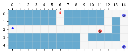
Figure 1: Multi-agent system collision avoidance benchmark with random ordered tasks, one-way lane, and model $\mathscr{M}_{11}$.

VII-F Multi-Agent System Collision Avoidance with Random Ordered Task and One-Way Lane

In the experiment of this subsection, there are two agents $A_{1}$ and $A_{2}$. Their transitions in the gridworld are again deterministic and their locations are known to both the agents. Agent $A_{1}$ has one goal location $a$ and agent $A_{2}$ has two goal locations $b$ and $c$ (both of which are active at all times). An agent receives a positive reward only when it is at its goal locations. We require agent $A_{2}$ to visit both its goal locations, but in a specific order (i.e., $b$ to $c$ or $c$ to $b$). The goal locations are known to both agents but the desired visitation order is known only to agent $A_{2}$. This order is randomly chosen at the beginning and kept fixed (indicated by the truth value of $o$). We again require the agents to avoid collision and stay in the lanes as in the previous section. This requirements can be specified using $\textsc{LTL}_{f}$ as $\varphi_{7}=(o\to(\neg b\textbf{U}(c\wedge\textbf{F}b)))\wedge(\neg o\to(\neg c\textbf{U}(b\wedge\textbf{F}c)))\wedge(\textbf{G}(s\wedge\neg col))$. We use a larger grid size of $5\times 15$ with a more complex lane structure. Further, we allow only one-way movement in some lanes. This task was performed on model $\mathscr{M}_{11}$.

For each model discussed above, we use Algorithm 1 to generate a mixed policy $\bar{\mu}$. The corresponding reward $\mathcal{R}^{\mathscr{M}}(\bar{\mu})$ and the constraint $\mathcal{R}^{f}(\bar{\mu})$ (estimated via $200$ Monte-Carlo simulations) are shown in Table I. We observe that the probability of satisfying the constraint generally exceeds the required threshold. Occasionally, the constraint is violated albeit only by a small margin. This is consistent with our result in Theorem 2. Since we cannot exactly compute the optimal feasible reward $\mathcal{R}^{*}$, it is difficult to assess how close our policy is to optimality. Nonetheless, we observe that the agent behaves in a manner that achieves high reward in all of these models. A detailed discussion of the experimental setup is available in Appendix F.

VIII Conclusions

We provided a methodology for designing agent policies that maximize the total expected reward while ensuring that the probability of satisfying a linear temporal logic ($\textsc{LTL}_{f}$) specification is sufficiently high. By augmenting the system state with the state of the DFA associated with the $\textsc{LTL}_{f}$ specification, we constructed a constrained product POMDP. Solving this constrained product POMDP is equivalent to solving the original problem. We provided an alternative constrained POMDP solver based on the exponentiated gradient (EG) algorithm and derived approximation bounds for it. Our methodology is further extended to a multi-agent setting with information asymmetry. For these various settings, we computed near optimal policies that satisfy the $\textsc{LTL}_{f}$ specification with sufficiently high probability. We observed in our experiments that our approach results in policies that effectively balance information acquisition (exploration), reward maximization (exploitation) and satisfaction of the specification which is very difficult to achieve using classical POMDPs.

Appendix A Proof of Theorem 1

For any policy $\mu$, we have

$$\mathcal{R}^{\mathscr{M}^{\times}}_{o}(\mu) ={\mathbb{E}}_{\mu}\left[\sum_{t=0}^{T}r_{t}^{o\times}(X_{t},{\mathcal{U}}_{t})\right]$$

$$={\mathbb{E}}_{\mu}\left[\sum_{t=0}^{T}r_{t}^{o\times}((\mathcal{S}_{t},Q_{t}),{\mathcal{U}}_{t})\right]$$

$$\stackrel{{\scriptstyle a}}{{=}}{\mathbb{E}}_{\mu}\left[\sum_{t=0}^{T}r_{t}^{o}(\mathcal{S}_{t},{\mathcal{U}}_{t})\right]=\mathcal{R}^{\mathscr{M}}_{o}(\mu).$$

The equality in $(a)$ follows from the definition of $r_{t}^{o\times}$ in (8). We can similarly show that $\mathcal{R}^{\mathscr{M}^{\times}}_{c}(\mu)=\mathcal{R}^{\mathscr{M}}_{c}(\mu)$. Further, using (VI-B), we have

$$r^{f}(X_{T+1}) =r^{f}((\mathcal{S}_{T+1},Q_{T+1}))=\mathds{1}_{F}(Q_{T+1}).$$

By construction of the product POMDP dynamics, a run $X_{0:T}$ of the product POMDP satisfies $\varphi$ if and only $Q_{T+1}\in F$. Hence,

$$\mathcal{R}^{f}(\mu)={\mathbb{E}}_{\mu}\left[r^{f}(X_{T+1})\right]={\mathbb{P}}_{\mu}^{\mathcal{M}}(\varphi).$$

Appendix B Proof of Lemma 1

By definition of the Lagrangian function for Problem (P2), we have:

$$\mathcal{R}^{*} =l^{*}$$

$$\leq l^{*}_{B}$$

$$\leq\inf_{\boldsymbol{\lambda}\geq 0,\lVert\boldsymbol{\lambda}\rVert_{1}\leq B}L(\bar{\mu},\boldsymbol{\lambda})+\epsilon$$

$$=\epsilon+\mathcal{R}^{\mathscr{M}^{\times}}_{o}(\bar{\mu})+$$ (35)

$$\inf_{\boldsymbol{\lambda}\geq 0,\lVert\boldsymbol{\lambda\rVert}_{1}\leq B}\left[\lambda^{f}(\mathcal{R}^{f}(\bar{\mu})-1+\delta)+\lambda^{c}(\mathcal{R}^{\mathscr{M}^{\times}}_{c}(\bar{\mu})-\rho)\right].$$

There are two possible cases:
(i) $\min\{\mathcal{R}^{f}(\bar{\mu})-1+\delta,\mathcal{R}^{\mathscr{M}^{\times}}_{c}(\bar{\mu})-\rho\}\geq 0$ and
(ii) $\min\{\mathcal{R}^{f}(\bar{\mu})-1+\delta,\mathcal{R}^{\mathscr{M}^{\times}}_{c}(\bar{\mu})-\rho\}<0$.

If case (i) is true, then (16) and (17) are trivially satisfied. Further, in this case,

$$\inf_{\boldsymbol{\lambda}\geq 0,\lVert\boldsymbol{\lambda\rVert}_{1}\leq B}\left[\lambda^{f}(\mathcal{R}^{f}(\bar{\mu})-1+\delta)+\lambda^{c}(\mathcal{R}^{\mathscr{M}^{\times}}_{c}(\bar{\mu})-\rho)\right]=0.$$

Therefore, $\mathcal{R}^{*}\leq\mathcal{R}^{\mathscr{M}^{\times}}_{o}(\bar{\mu})+\epsilon$ holds, hence (15) is satisfied.

If case (ii) is true, we have

$$\inf_{\boldsymbol{\lambda}\geq 0,\lVert\boldsymbol{\lambda\rVert}_{1}\leq B}\left[\lambda^{f}(\mathcal{R}^{f}(\bar{\mu})-1+\delta)+\lambda^{c}(\mathcal{R}^{\mathscr{M}^{\times}}_{c}(\bar{\mu})-\rho)\right]$$

$$=B\min\{\mathcal{R}^{f}(\bar{\mu})-1+\delta,\mathcal{R}^{\mathscr{M}^{\times}}_{c}(\bar{\mu})-\rho\}<0$$ (36)

The results in (35) and (36) together imply that $\mathcal{R}^{*}\leq\mathcal{R}^{\mathscr{M}^{\times}}_{o}(\bar{\mu})+\epsilon$ and hence, (15) is satisfied. Further, by substituting (36) in (35) we get

$$B\min\{\mathcal{R}^{f}(\bar{\mu})-1+\delta,\mathcal{R}^{\mathscr{M}^{\times}}_{c}(\bar{\mu})-\rho\} \geq\mathcal{R}^{*}-\mathcal{R}^{\mathscr{M}^{\times}}_{o}(\bar{\mu})-\epsilon$$

$$\geq\mathcal{R}^{*}-R_{m}-\epsilon,$$

where the last inequality holds because $R_{m}$ is the maximum possible reward. Hence, (16) and (17) are satisfied.

Appendix C Proof of Theorem 2

Consider the dual of (P4) and define

$$u^{*}_{B}:=\inf_{\boldsymbol{\lambda}\geq 0,\lVert\boldsymbol{\lambda}\rVert_{1}\leq B}\sup_{\mu}L(\mu,\boldsymbol{\lambda}).$$ (P7)

Then, we obtain $l^{*}_{B}\stackrel{{\scriptstyle a}}{{\leq}}u^{*}_{B}$ and

$$u^{*}_{B} =\inf_{\boldsymbol{\lambda}\geq 0,\lVert\boldsymbol{\lambda}\rVert_{1}\leq B}\sup_{\mu}L(\mu,\boldsymbol{\lambda})$$

$$\stackrel{{\scriptstyle}}{{\leq}}\sup_{\mu}L(\mu,\bar{\boldsymbol{\lambda}})$$

$$\stackrel{{\scriptstyle}}{{=}}L(\mu_{\bar{\boldsymbol{\lambda}}},\bar{\boldsymbol{\lambda}})$$

$$\stackrel{{\scriptstyle b}}{{=}}\frac{1}{K}\sum_{k=1}^{K}L(\mu_{\bar{\boldsymbol{\lambda}}},{\boldsymbol{\lambda}}_{k})$$

$$\stackrel{{\scriptstyle c}}{{\leq}}\frac{1}{K}\sum_{k=1}^{K}L(\mu_{k},{\boldsymbol{\lambda}}_{k})$$

$$\stackrel{{\scriptstyle d}}{{\leq}}\frac{1}{K}\inf_{\boldsymbol{\lambda}\geq 0,\lVert\boldsymbol{\lambda}\rVert_{1}\leq B}\sum_{k=1}^{K}L(\mu_{k},{\boldsymbol{\lambda}})+2BG\sqrt{2\log 3/K}$$

$$\stackrel{{\scriptstyle e}}{{=}}\inf_{\boldsymbol{\lambda}\geq 0,\lVert\boldsymbol{\lambda}\rVert_{1}\leq B}L(\bar{\mu},{\boldsymbol{\lambda}})+2BG\sqrt{2\log 3/K}.$$ (37)

The inequality in $(a)$ holds because of weak duality [31]. The equality in $(b)$ holds because $L(\cdot,\cdot)$ is a bilinear (more precisely, bi-affine) function. The inequality in $(c)$ holds because $\mu_{k}$ is the maximizer associated with $\boldsymbol{\lambda}_{k}$. Inequality $(d)$ follows from the no-regret property of the EG algorithm [30, Corollary 5.7]. The equality in $(e)$ is again a consequence of the bilinearity of $L(\cdot,\cdot)$. Combining (37) with Lemma 1 proves the theorem.

Appendix D Proof of Theorem 3

Define $\hat{L}(\mu,\boldsymbol{\lambda})=\mathcal{R}^{\mathscr{M}^{\times}}(\mu)+\lambda^{f}(\textsc{eval}(\mu,r^{f})-1+\delta)+\lambda^{c}(\textsc{eval}(\mu,r^{c\times})-\rho)$. Following initial arguments similar to those in the proof of Theorem 2, we obtain:

$$l^{*}_{B} \stackrel{{\scriptstyle}}{{\leq}}\frac{1}{K}\sum_{k=1}^{K}L(\mu_{\bar{\boldsymbol{\lambda}}},{\boldsymbol{\lambda}}_{k})$$

$$\stackrel{{\scriptstyle a}}{{\leq}}\frac{1}{K}\sum_{k=1}^{K}L(\mu_{\boldsymbol{\lambda}_{k}},{\boldsymbol{\lambda}}_{k})$$

$$\stackrel{{\scriptstyle b}}{{\leq}}\frac{1}{K}\sum_{k=1}^{K}L(\mu_{k},{\boldsymbol{\lambda}}_{k})+\epsilon_{bp}$$

$$\stackrel{{\scriptstyle c}}{{\leq}}\frac{1}{K}\sum_{k=1}^{K}\hat{L}(\mu_{k},{\boldsymbol{\lambda}}_{k})+\epsilon_{bp}+\epsilon_{est}$$

$$\stackrel{{\scriptstyle d}}{{\leq}}\frac{1}{K}\inf_{\boldsymbol{\lambda}\geq 0,\lVert\boldsymbol{\lambda}\rVert_{1}\leq B}\sum_{k=1}^{K}\hat{L}(\mu_{k},{\boldsymbol{\lambda}})+2BG\sqrt{\frac{2\log 3}{K}}+\epsilon_{bp}+\epsilon_{est}$$

$$\stackrel{{\scriptstyle e}}{{=}}\inf_{\boldsymbol{\lambda}\geq 0,\lVert\boldsymbol{\lambda}\rVert_{1}\leq B}\hat{L}(\bar{\mu},{\boldsymbol{\lambda}})+2BG\sqrt{2\log 3/K}+\epsilon_{bp}+\epsilon_{est}$$

$$\stackrel{{\scriptstyle f}}{{\leq}}\inf_{\boldsymbol{\lambda}\geq 0,\lVert\boldsymbol{\lambda}\rVert_{1}\leq B}L(\bar{\mu},{\boldsymbol{\lambda}})+2BG\sqrt{2\log 3/K}+\epsilon_{bp}+2\epsilon_{est}.$$ (38)

The inequality in $(a)$ holds because $\mu_{\boldsymbol{\lambda}_{k}}$ is the maximizer associated with $\boldsymbol{\lambda}_{k}$. The inequality in $(b)$ holds by the bounded sub-optimality of $\mu_{k}$. Inequality $(c)$ follows from the bounded error of the estimator. Inequality $(d)$ follows from the no-regret property of the EG algorithm. The equality in $(e)$ is again a consequence of the bilinearity of $\hat{L}(\cdot)$. Finally, inequality $(f)$ follows from the bounded error of the estimator. Combining (38) with Lemma 1 proves the theorem.

Appendix E Proof of Lemma 2

The rewards $\mathcal{R}^{\mathscr{M}^{\times}}_{o}(\mu)$ and $\mathcal{R}^{f}(\mu)$ in the corresponding product POMDP are given by

$$\mathcal{R}^{\mathscr{M}^{\times}}_{o}(\mu) ={\mathbb{E}}_{\mu}\left[\sum_{t=0}^{T}r_{t}^{o\times}(X_{t},{\mathcal{U}}_{t})\right]$$

$$=(1-\gamma){\mathbb{E}}_{\mu}\left[\sum_{k=0}^{\infty}\gamma^{k}\sum_{t=0}^{k}r_{t}^{o\times}(X_{t},{\mathcal{U}}_{t})\right]$$

$$=(1-\gamma){\mathbb{E}}_{\mu}\left[\sum_{t=0}^{\infty}\sum_{k=0}^{\infty}\gamma^{k+t}r_{t}^{o\times}(X_{t},{\mathcal{U}}_{t})\right]$$

$$={\mathbb{E}}_{\mu}\left[\sum_{t=0}^{\infty}\gamma^{t}r_{t}^{o\times}(X_{t},{\mathcal{U}}_{t})\right]$$

$$\mathcal{R}^{f}(\mu) ={\mathbb{E}}_{\mu}\left[r^{f}(X_{T+1})\right]$$

$$=(1-\gamma){\mathbb{E}}_{\mu}\left[\sum_{t=0}^{\infty}\gamma^{t}r^{f}(X_{t+1})\right]$$

$$=\frac{(1-\gamma)}{\gamma}{\mathbb{E}}_{\mu}\left[\sum_{t=1}^{\infty}\gamma^{t}r^{f}(X_{t})\right].$$

Similarly, we have $\mathcal{R}^{\mathscr{M}^{\times}}_{c}(\mu)={\mathbb{E}}_{\mu}\left[\sum_{t=0}^{\infty}\gamma^{t}r_{t}^{c\times}(X_{t},{\mathcal{U}}_{t})\right]$. Therefore,

$$L(\mu,\boldsymbol{\lambda})=-\frac{\lambda^{f}(1-\gamma)}{\gamma}{\mathbb{E}}[r^{f}(X_{0})]-\lambda^{f}(1-\delta)-\lambda^{c}\rho+$$

$${\mathbb{E}}_{\mu}\left[\sum_{t=0}^{\infty}\gamma^{t}\left(r_{t}^{o\times}(X_{t},{\mathcal{U}}_{t})+\frac{\lambda^{f}(1-\gamma)}{\gamma}r^{f}(X_{t})+\lambda^{c}r_{t}^{c\times}(X_{t},{\mathcal{U}}_{t})\right)\right].$$

Appendix F Additional Details on Experiments

In this subsection, we provide further details on the grid world POMDP models used in our experiments. The images corresponding to the various models indicate the grid space and the associated labeling function, e.g., in Fig. 2(c), we have $L[(5,2)],L[(1,6)]=\{b\},L[(7,7)]=\{a\}$ and $L[(i,j)]=\{\}$ for all other grid locations $(i,j)$. In all single agent models, the agent starts from the grid location $(0,0)$. Further, the default reward for all actions is $0$ in all grid locations, unless specified otherwise.

F-A Single-Agent Location Uncertainty

In the experiments of this section, if the agent decides to move in a certain direction, it moves in that direction with probability $0.95$ and, with probability $0.05$, it randomly moves one step in any direction that is not opposite to its intended direction.

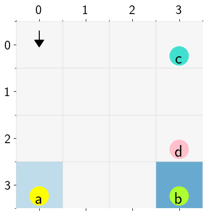
(a) Model $\mathscr{M}_{3}$ Reactive Task.

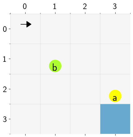
(b) Model $\mathscr{M}_{2}$ Ordered Task.

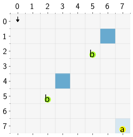
(c) Model $\mathscr{M}_{1}$ Reach-Avoid Task.

Figure 2: Single-Agent Location Uncertainty.

In model $\mathscr{M}_{1}$, reward $r((1,6),u)=3,r((4,3),u)=3$ and $r((7,7),u)=1$ for all actions $u$. In model $\mathscr{M}_{2}$, reward $r((3,3),u)=1$ for all actions $u$. In model $\mathscr{M}_{3}$, reward $r((3,0),u)=1$ and $r((3,3),u)=2$ for all actions $u$.

F-B Single-Agent Predicate Uncertainty

In the experiments of this section, there are two possible locations for object $b$: $(3,0)$ and $(0,3)$. In both cases, whenever the agent is ‘far’ away (Manhattan distance greater than 1) from the object $b$, it gets an observation ‘F’ indicating that it is far with probability $1$. When the object is at the bottom left and the agent is adjacent to it, the agent gets an observation ‘C’ with probability $0.9$ indicating that the object is close. But if object $b$ is at the top right and the agent is adjacent to it, the agent gets an observation ‘C’ only with probability $0.1$. Therefore, the detection capability of the agent is stronger when the object is in the bottom-left location as opposed to when it is in the top-right location.

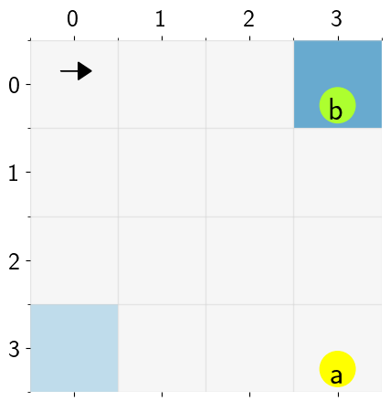
(a) Model $\mathscr{M}_{4}$ with obstacle at $(0,3)$.

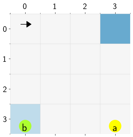
(b) Model $\mathscr{M}_{4}$ with obstacle at $(3,0)$.

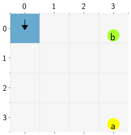
(c) Model $\mathscr{M}_{5}$ with obstacle at $(0,3)$.

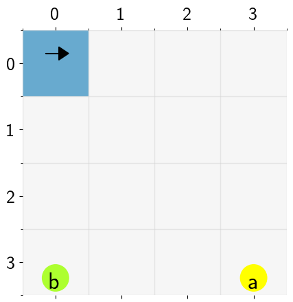
(d) Model $\mathscr{M}_{5}$ with obstacle at $(3,0)$.

Figure 3: Single-Agent Predicate Uncertainty.

In model $\mathscr{M}_{4}$, reward $r((3,0),u)=2$ and $r((0,3),u)=4$ for all actions $u$. In model $\mathscr{M}_{5}$, reward $r((0,0),u)=2$ for all actions $u$.

F-C Goal-POMDPs Location Uncertainty

In the experiments of this subsection, the agent moves in the intended direction with probability $0.8$ and, with probability $0.2$, it moves one step with uniform probability in any direction that is not opposite to its intended direction.

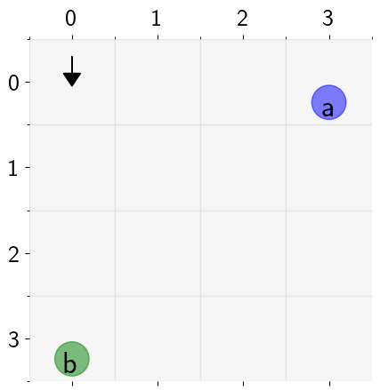
(a) Model $\mathscr{M}_{6}$ Ordered Task with Automaton Goal.

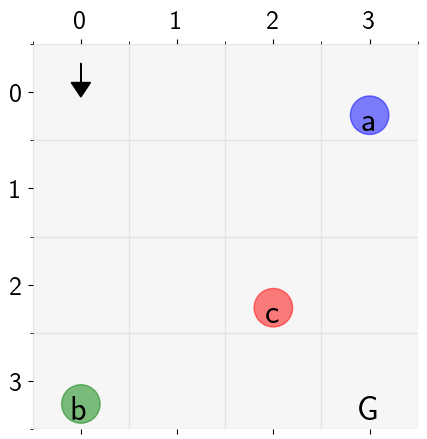
(b) Model $\mathscr{M}_{8}$ Random Ordered Task with Gridworld Goal.

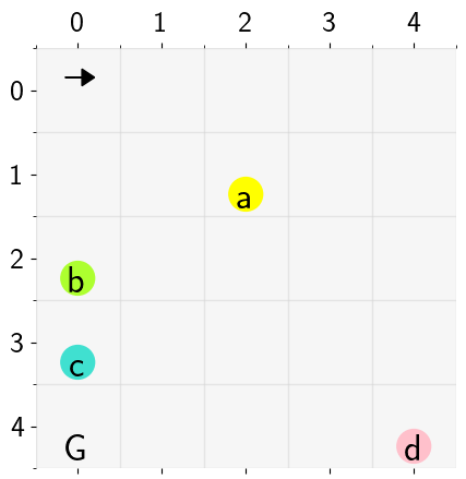
(c) Model $\mathscr{M}_{7}$ Reach-Avoid Reactive Task.

Figure 4: Goal-POMDPs.

In model $\mathscr{M}_{6}$, the goal state for the agent is not shown in the image as it is not a grid location. Further, since the goal state is the accept state of the DFA, we observe that the specification is satisfied with probability $1$. In model $\mathscr{M}_{7}$, the goal state for the agent is the grid location $(4,0)$.

F-D Goal-POMDPs Specification Uncertainty

The observation corresponding to grid location $(2,2)$ provides the truth value of $c$. This determines the order of visiting $a$ and $b$. In model $\mathscr{M}_{8}$, the goal state for the agent is the grid location $(3,3)$.

F-E Multi-Agent System Collision Avoidance

In the figures associated with this section, the lanes are shown by the grey grid cells. In all experiments of this section, agent $A_{1}$ starts from $(0,2)$ and agent $A_{2}$ starts from $(2,0)$.

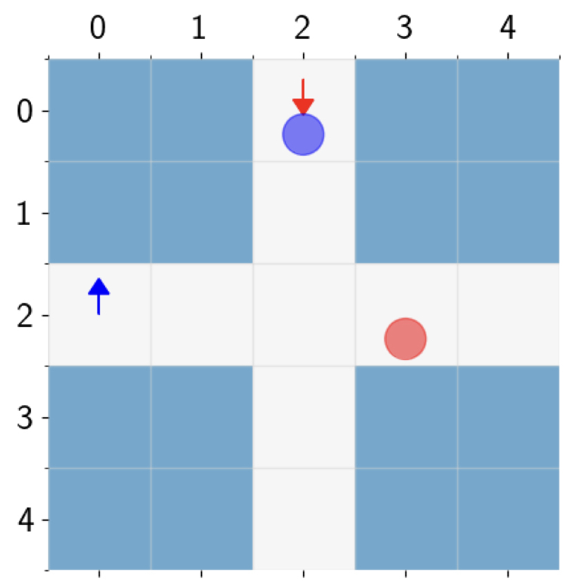
(a) Model $\mathscr{M}_{9}$ One Agent Goal Switching.

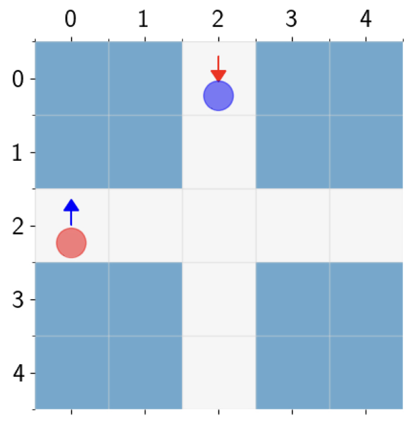
(b) Model $\mathscr{M}_{10}$ Two Agents Goal Switching.

Figure 5: Multi-Agent System Collision Avoidance.

One Agent Goal Switching

In model $\mathscr{M}_{9}$, agent $A_{1}$ (red arrow) has only one goal location $a$ (2, 3) and agent $A_{2}$ (blue arrow)’s goal location switches between $b$ (0, 2), $c$ (2, 4), and $d$ (4, 2). Agent $A_{1}$ gets a reward of $1$ for each time-step in its goal location whereas agent $A_{2}$ gets a reward of $3$ for each time-step in any of its goal locations.

Such a reward structure incentivizes agent $A_{1}$ to move away from its goal location $a$ (2, 3) when agent $A_{2}$ has its goal location at $c$ (2,4). This is to avoid collision and attain higher reward. Our results match this expectation: agent $A_{1}$ stays in (2, 3) as long as possible, except when agent $A_{2}$ has to pass by to reach (2, 4), in which cases $A_{1}$ will move and let $A_{2}$ pass.

Two Agents Goal Switching

In model $\mathscr{M}_{10}$, agent $A_{1}$ (red arrow) has two possible goal locations $a$ (2, 0), $b$ (2, 4) and agent $A_{2}$ (blue arrow) has two possible goal locations $c$ (0, 2), $d$ (4, 2). Either agent receives a reward of $1$ for each time-step in its own goal location.

F-F Multi-Agent System Collision Avoidance with Random Ordered Task and One-Way Lane

In model $\mathscr{M}_{11}$, agent $A_{2}$ (blue arrow) starting from $(2,0)$ has two goal locations $b$ (0, 14) and $c$ (4, 14), while agent $A_{1}$ (red arrow) starting from $(0,6)$ has one goal location $a$ (2, 11). Either agent receives a reward of $1$ for each time-step in their own goal locations. The environment allows only one-way movement in the lane from $(4,14)$ to $(0,14)$. Thus, if $o$ indicates that agent $A_{2}$ has to visit $c$ before $b$, it can do so through the one-way lane between $c$ and $b$. But, if $o$ indicates the other order of visitation, then agent $A_{2}$ has to take the longer route from $b$ to $c$ which passes through agent $A_{1}$’s goal location i.e., (2, 11). Our result matches this expectation, with the agents moving in a manner so as to avoid collision and maximize total reward.

Figure 6: Multi-agent system collision avoidance benchmark with random ordered tasks, one-way lane, and model $\mathscr{M}_{11}$.

References

• [1] M.ย L. Puterman, Markov Decision Processes: Discrete Stochastic Dynamic Programming, 1stย ed.ย ย ย New York, NY, USA: John Wiley & Sons, Inc., 1994.
• [2] C.ย Baier and J.-P. Katoen, Principles of Model Checking.ย ย ย MIT press, 2008.
• [3] D.ย P. Bertsekas, D.ย P. Bertsekas, D.ย P. Bertsekas, and D.ย P. Bertsekas, Dynamic programming and optimal control.ย ย ย Athena scientific Belmont, MA, 1995, vol.ย 1.
• [4] G.ย Deย Giacomo and M.ย Y. Vardi, โ€œLinear temporal logic and linear dynamic logic on finite traces,โ€ in Twenty-Third International Joint Conference on Artificial Intelligence, 2013.
• [5] S.ย Zhu, L.ย M. Tabajara, J.ย Li, G.ย Pu, and M.ย Y. Vardi, โ€œSymbolic LTLf synthesis,โ€ arXiv preprint arXiv:1705.08426, 2017.
• [6] H.ย Kurniawati, D.ย Hsu, and W.ย S. Lee, โ€œSARSOP: Efficient point-based POMDP planning by approximating optimally reachable belief spaces,โ€ in Robotics: Science and systems, vol. 2008.ย ย ย Citeseer, 2008.
• [7] D.ย Silver and J.ย Veness, โ€œMonte-Carlo planning in large POMDPs,โ€ Advances in neural information processing systems, vol.ย 23, 2010.
• [8] A.ย Nayyar, A.ย Mahajan, and D.ย Teneketzis, โ€œDecentralized Stochastic Control with Partial History Sharing: A Common Information Approach,โ€ IEEE Transactions on Automatic Control, vol.ย 58, no.ย 7, pp. 1644โ€“1658, 2013.
• [9] K.ย C. Kalagarla, K.ย Dhruva, D.ย Shen, R.ย Jain, A.ย Nayyar, and P.ย Nuzzo, โ€œOptimal Control of Partially Observable Markov Decision Processes with Finite Linear Temporal Logic Constraints,โ€ in Uncertainty in Artificial Intelligence.ย ย ย PMLR, 2022, pp. 949โ€“958.
• [10] X.ย C.ย D. Ding, S.ย L. Smith, C.ย Belta, and D.ย Rus, โ€œLTL control in uncertain environments with probabilistic satisfaction guarantees,โ€ IFAC Proceedings Volumes, vol.ย 44, no.ย 1, pp. 3515โ€“3520, 2011.
• [11] S.ย Sickert, J.ย Esparza, S.ย Jaax, and J.ย Kล™etรญnskแปณ, โ€œLimit-Deterministic Bรผchi Automata for Linear Temporal Logic,โ€ in International Conference on Computer Aided Verification.ย ย ย Springer, 2016, pp. 312โ€“332.
• [12] E.ย M. Hahn, M.ย Perez, S.ย Schewe, F.ย Somenzi, A.ย Trivedi, and D.ย Wojtczak, โ€œOmega-Regular Objectives in Model-Free Reinforcement Learning,โ€ in International Conference on Tools and Algorithms for the Construction and Analysis of Systems, 2019, pp. 395โ€“412.
• [13] A.ย K. Bozkurt, Y.ย Wang, M.ย M. Zavlanos, and M.ย Pajic, โ€œControl synthesis from linear temporal logic specifications using model-free reinforcement learning,โ€ arXiv preprint arXiv:1909.07299, 2019.
• [14] S.ย Haesaert, P.ย Nilsson, C.ย I. Vasile, R.ย Thakker, A.-a. Agha-mohammadi, A.ย D. Ames, and R.ย M. Murray, โ€œTemporal logic control of POMDPs via label-based stochastic simulation relations,โ€ IFAC-PapersOnLine, vol.ย 51, no.ย 16, pp. 271โ€“276, 2018.
• [15] G.ย Norman, D.ย Parker, and X.ย Zou, โ€œVerification and control of partially observable probabilistic real-time systems,โ€ in International Conference on Formal Modeling and Analysis of Timed Systems.ย ย ย Springer, 2015, pp. 240โ€“255.
• [16] M.ย Ahmadi, R.ย Sharan, and J.ย W. Burdick, โ€œStochastic finite state control of POMDPs with LTL specifications,โ€ arXiv preprint arXiv:2001.07679, 2020.
• [17] R.ย Sharan and J.ย Burdick, โ€œFinite state control of POMDPs with LTL specifications,โ€ in 2014 American Control Conference.ย ย ย IEEE, 2014, pp. 501โ€“508.
• [18] J.ย Liu, E.ย Rosen, S.ย Zheng, S.ย Tellex, and G.ย Konidaris, โ€œLeveraging Temporal Structure in Safety-Critical Task Specifications for POMDP Planning,โ€ 2021.
• [19] M.ย Bouton, J.ย Tumova, and M.ย J. Kochenderfer, โ€œPoint-based methods for model checking in partially observable Markov decision processes,โ€ in Proceedings of the AAAI Conference on Artificial Intelligence, 2020.
• [20] S.ย Carr, N.ย Jansen, and U.ย Topcu, โ€œVerifiable RNN-based policies for POMDPs under temporal logic constraints,โ€ arXiv preprint arXiv:2002.05615, 2020.
• [21] S.ย Carr, N.ย Jansen, R.ย Wimmer, A.ย C. Serban, B.ย Becker, and U.ย Topcu, โ€œCounterexample-guided strategy improvement for POMDPs using recurrent neural networks,โ€ arXiv preprint arXiv:1903.08428, 2019.
• [22] P.ย Poupart, A.ย Malhotra, P.ย Pei, K.-E. Kim, B.ย Goh, and M.ย Bowling, โ€œApproximate linear programming for constrained partially observable Markov decision processes,โ€ in Proceedings of the AAAI Conference on Artificial Intelligence, vol.ย 29, no.ย 1, 2015.
• [23] J.ย Lee, G.-H. Kim, P.ย Poupart, and K.-E. Kim, โ€œMonte-Carlo tree search for constrained POMDPs,โ€ Advances in Neural Information Processing Systems, vol.ย 31, 2018.
• [24] E.ย Walraven and M.ย T. Spaan, โ€œColumn generation algorithms for constrained POMDPs,โ€ Journal of artificial intelligence research, vol.ย 62, pp. 489โ€“533, 2018.
• [25] L.ย Hammond, A.ย Abate, J.ย Gutierrez, and M.ย Wooldridge, โ€œMulti-agent reinforcement learning with temporal logic specifications,โ€ arXiv preprint arXiv:2102.00582, 2021.
• [26] W.ย Wang, G.ย F. Schuppe, and J.ย Tumova, โ€œDecentralized multi-agent coordination under mitl tasks and communication constraints,โ€ in 2022 ACM/IEEE 13th International Conference on Cyber-Physical Systems (ICCPS).ย ย ย IEEE, 2022, pp. 320โ€“321.
• [27] J.ย Eappen and S.ย Jagannathan, โ€œDistSPECTRL: Distributing Specifications in Multi-Agent Reinforcement Learning Systems,โ€ arXiv preprint arXiv:2206.13754, 2022.
• [28] N.ย Zhang, W.ย Liu, and C.ย Belta, โ€œDistributed Control using Reinforcement Learning with Temporal-Logic-Based Reward Shaping,โ€ in Learning for Dynamics and Control Conference.ย ย ย PMLR, 2022, pp. 751โ€“762.
• [29] C.ย Sun, X.ย Li, and C.ย Belta, โ€œAutomata guided semi-decentralized multi-agent reinforcement learning,โ€ in 2020 American Control Conference (ACC).ย ย ย IEEE, 2020, pp. 3900โ€“3905.
• [30] E.ย Hazan etย al., โ€œIntroduction to online convex optimization,โ€ Foundations and Trendsยฎ in Optimization, vol.ย 2, no. 3-4, pp. 157โ€“325, 2016.
• [31] S.ย Boyd and L.ย Vandenberghe, Convex optimization.ย ย ย Cambridge university press, 2004.
• [32] K.ย Horรกk, B.ย Bosanskแปณ, and K.ย Chatterjee, โ€œGoal-HSVI: Heuristic Search Value Iteration for Goal POMDPs.โ€ in IJCAI, 2018, pp. 4764โ€“4770.
• [33] A.ย Mahajan, โ€œOptimal Decentralized Control of Coupled Subsystems With Control Sharing,โ€ IEEE Transactions on Automatic Control, vol.ย 58, no.ย 9, pp. 2377โ€“2382, 2013.
• [34] D.ย Kartik, S.ย Sudhakara, R.ย Jain, and A.ย Nayyar, โ€œOptimal communication and control strategies for a multi-agent system in the presence of an adversary,โ€ in 2022 IEEE 61st Conference on Decision and Control (CDC).ย ย ย IEEE, 2022, pp. 4155โ€“4160.
• [35] F.ย Fuggitti, โ€œLtlf2dfa,โ€ Mar. 2019. [Online]. Available: https://doi.org/10.5281/zenodo.3888410
• [36] N.ย Klarlund and A.ย Mรธller, MONA Version 1.4 User Manual, BRICS, Department of Computer Science, University of Aarhus, January 2001, notes Series NS-01-1. Available from http://www.brics.dk/mona/.