PruMUX: Augmenting Data Multiplexing with Model Compression

Abstract

As language models increase in size by the day, methods for efficient inference are critical to leveraging their capabilities for various applications. Prior work has investigated techniques like model pruning, knowledge distillation, and data multiplexing to increase model throughput without sacrificing accuracy. In this paper, we combine two such methods – structured pruning and data multiplexing – to compound the speedup gains obtained by either method. Our approach, PruMUX, obtains up to 7.5-29.5X throughput improvement over BERT-base model with accuracy threshold from 80% to 74%. We further study various combinations of parameters (such as sparsity and multiplexing factor) in the two techniques to provide a comprehensive analysis of the tradeoff between accuracy and throughput in the resulting models. We then propose Auto-PruMUX, a meta-level model that can predict the high-performance parameters for pruning and multiplexing given a desired accuracy loss budget, providing a practical method to leverage the combination effectively.

1 Introduction

Large language models (LLMs) have achieved state-of-the-art performance across various NLP tasks and resulted in impressive user-facing demonstrations such as ChatGPT. However, their large size necessitates the use of enormous amounts of compute and memory at inference time, which limits their widespread use.

Two types of techniques have been explored to reduce the cost of model inference. The first is model compression including network pruning LeCun et al. (1989); Han et al. (2015b); Frankle and Carbin (2019), quantization Han et al. (2016), knowledge distillation Hinton et al. (2015), combinations of multiple methods Xia et al. (2022). The second is recently proposed data multiplexing Murahari et al. (2023), which multiplexes multiple inputs into a single input for model inference.

While both types of methods leverage the over-parameterization effect Allen-Zhu et al. (2019); Radhakrishnan et al. (2020) in modern deep neural networks to improve the throughput-to-compute cost ratio, the manner in which they do so is different. Model compression aims at reducing the number of parameters in the model, hence reducing the overall compute cost (denominator) to improve the ratio. Data multiplexing, on the other hand, compresses multiple inputs into one to improve throughput (numerator) while keeping the model size fixed. This observation naturally leads us to hypothesize that the two types of methods could be complementary and can be combined for maximal gain in the throughput-to-compute cost ratio.

Figure 1: Throughput improvements ($\times$) of CoFi, DataMUX, and PruMUX over the BERT-base model Devlin et al. (2018) on the MNLI task Williams et al. (2017). The sparsity for a CoFi’s data point is labeled as $s$. The width of multiplexing for a DataMUX’s data point is labeled as $N$. The parameter pair for a PruMUX’s data point is labeled as ($N$, $s$).

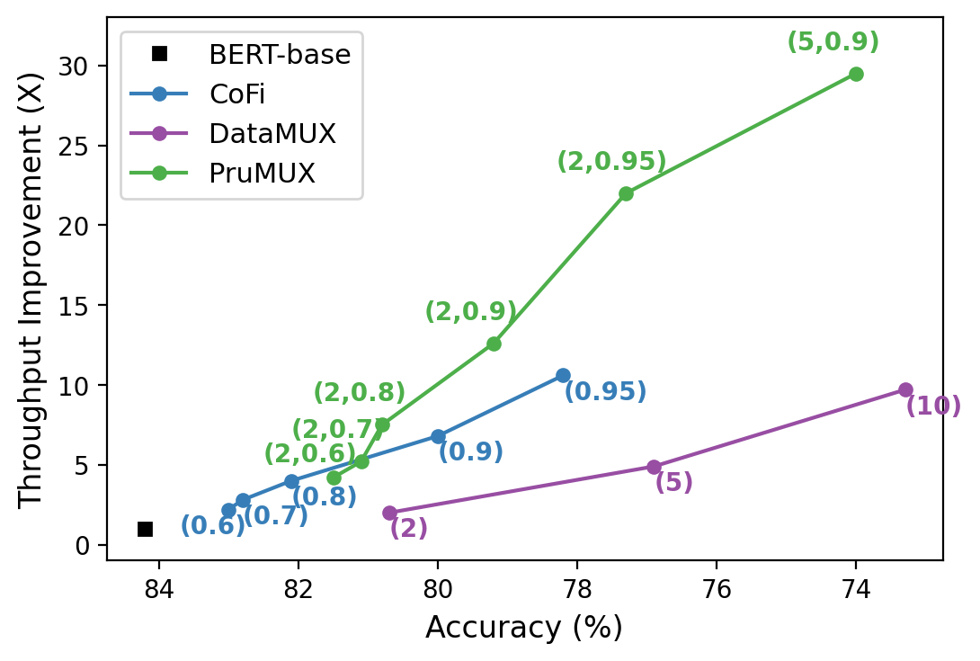
There are two challenges to this hypothesis. The first is that both model compression and data multiplexing aim at trading a small accuracy loss for large throughput improvement. Intuitively, the combination may incur an accuracy loss larger than either method and it is not clear how they interact with each other when combining them together. A research question is how to combine the two methods such that the combination achieves better throughput than each type of method individually, given any accuracy loss budget or accuracy threshold.

The second challenge is to efficiently find the best parameters pair ($N,s$) where $N$ is the width of the data multiplexing and $s$ is the sparsity of the model compression method. Training and testing with each parameter combination is costly and time-consuming. A research question is how to automatically predict and find top parameters based on the model’s performance on one set of parameters.

To address the first research question, we present PruMUX, a combination of model compression and data multiplexing. Our method is simple and consists of three phases – multiplexed model pre-training, task-specific fine-tuning and task-specific model compression. In our implementation, we make use of CoFi Xia et al. (2022), a state-of-the-art model compression method that includes intermediate knowledge distillation steps that help minimize accuracy hits, and DataMUX Murahari et al. (2023), which performs vector-based input multiplexing over instances.

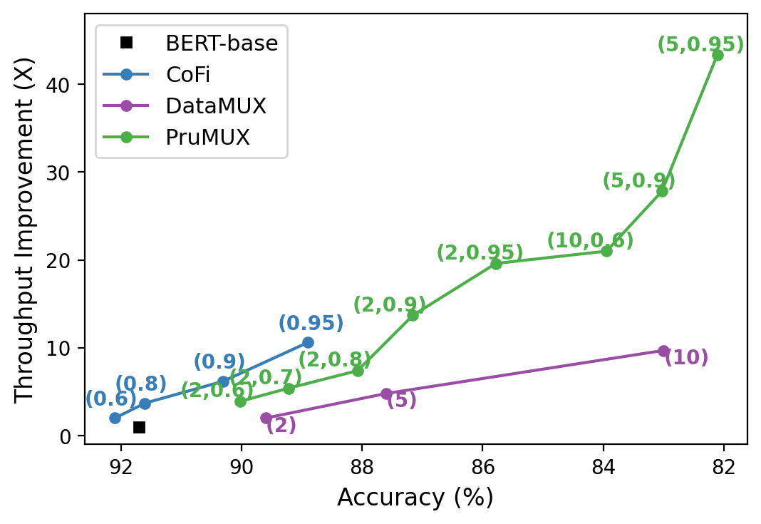
Our results over four datasets (MNLI, QNLI, QQP and SST-2) demonstrate that PruMUX achieves significantly higher throughput over CoFi and DataMUX individually for a large range of accuracy thresholds. As an example, Figure 1 shows the throughput improvements over the BERT-base model on task MNLI, providing a more optimal Pareto frontier in the tradeoff between accuracy and throughput.

To address the second research question, we propose Auto-PruMUX, a meta-model to automatically predict and find the high-performance parameter combinations for a desired accuracy loss budget on a task based on the model’s performance on one set of parameters without running additional experiments. We use interpolation and estimation models over a set of data points to predict the accuracy and throughput of a PruMUX model based on sparsity and multiplexing factor. We show promise in modeling the tradeoffs accurately and Auto-PruMUX can find high-performance combinations of known parameters as well as unknown parameters, providing a practical method for choosing a high-performance PruMUX model for a downstream task.

Our key insight for why PruMUX can achieve better throughput than model compression and data multiplexing individually is that they improve the throughput of a model in two different dimensions: reducing the latency of an inference and compressing multiple inferences. In addition, both methods lead to non-linear drops in model accuracy at some points. PruMUX can achieve high throughput while avoiding each method’s limitations.

2 Background

2.1 CoFi Pruning

CoFi is a state-of-the-art model compression method Xia et al. (2022) that uses distillation and structured pruning to jointly prune a Transformer network Devlin et al. (2018). Its key idea is to distill the knowledge from the base model into the pruned model during training. A layer-wise distillation approach is used to guide the pruning from the teacher model, i.e., dense model, to the student model, i.e., pruned model, with a loss defined as:

$$L_{layer}=\sum_{i\in\tau}MSE(W_{layer}\textbf{H}_{s}^{m(i)},\textbf{H}_{t}^{i})$$

where $\textbf{H}_{s}^{m(i)}$ and $\textbf{H}_{t}^{i}$ are hidden representations of the $m(i)$th feed-forward layer of the student model and $i$th feed-forward layer of the teacher model. $i$ is the teacher model’s closest layer to the layer $m(i)$ of the student model. $W_{layer}$ is a linear transformation matrix, initialized as an identity matrix.

CoFi prunes both coarse-grained and fine-grained units of the distilled network. The coarse-grained units include multi-head attention layers, fully-connected layers, and attention heads. The fine-grained units include hidden dimensions and intermediate dimensions of the Transformer model. Different masks are used for different pruning units and are learned via $\ell_{0}$ regularization during training. The units with mask variables smaller than a threshold are pruned away before inference.

2.2 DataMUX

Data multiplexing (DataMUX) is a recently proposed method Murahari et al. (2022, 2023) to compress multiple inputs into a single “mixed” representation of the same size as a single input to a network, in order to improve inference throughput. DataMUX introduces multiplexing layers, which multiplex different sequences into a single sequence of representations, i.e., multiplexed representations, and demultiplexing layers, which demultiplex/decompress the multiplexed representations. The multiplexed layer first compresses multiple input sequences into a single sequence of representations. These representations are then processed by a Transformer model and the resulting representations are then disentangled into independent representations by the demultiplexer layer. These representations are then used to make predictions. DataMUX, therefore, leads to a many-fold increase in inference throughput as just a single pass through the large Transformer model.

The multiplexing layer is defined as

$$\textbf{x}^{1:N}=\Phi(\textbf{x}^{1},...\textbf{x}^{N})=\frac{1}{N}\sum_{i=1}^{N}\phi^{i}(\textbf{x}^{i})$$

where x is the input sequence, $\phi^{i},i\in[1,...N]$, is the Hadamard product with a fixed Gaussian random vector and $N$ is the number of input sequences that get multiplexed. The multiplexed representations, $\textbf{x}^{1:N}$, are then processed by the Transformer model to generate hidden multiplexed representations, $\textbf{h}^{1:N}$.

The demultiplexer layer, in order to disentangle the hidden multiplexed representation, $\textbf{h}^{1:N}$, into independent representations, learns N parameterized demultiplexing functions, $\psi^{i}$. The independent representations, $\textbf{h}^{i}$, are then used to make predictions.

$$\textbf{h}^{i}=\psi^{i}(\textbf{h}^{1:N})\quad\forall i\in 1,2,...N$$

2.3 Observations

Both model compression and data multiplexing aim at trading small accuracy losses for large inference throughput improvements. When CoFi prunes a Transformer at relatively low sparsities, its accuracy loss is minimal and throughput improvement is significant, but at 95% sparsity, its accuracy loss becomes relatively significant Xia et al. (2022). DataMUX also shares this nonlinear property, as shown in Figure 1. In other words, the trade-off of each method is good only up to a certain point.

The two methods improve the throughput of a model in two dimensions. CoFi reduces the latency of an inference, whereas DataMUX compresses multiple inferences into one. A natural question is whether combining the two methods can achieve higher throughput with a smaller accuracy loss than each method individually.

3 PruMUX

Figure 2: Illustration of PruMUX showing a multiplexer, sparse Transformer, and a demultiplexer, with multiplexing width of 10, where 10 input sequences are mixed into 1 input sequence. The multiplexed Transformer model is pruned to reduce inference time. The training for PruMUX consists of three steps including retrieval warm-up, multiplexed model training, and Transformer pruning.

Our key motivational question is the following: given an accuracy loss budget, can the combination of model compression and data multiplexing achieve better throughput than each method individually? In this section, we first present PruMUX, a method to combine the two methods, and then show that PruMUX achieves substantially better throughput than each method alone for various accuracy thresholds in our experimental results.

3.1 Method

PruMUX is a method to convert any Transformer into a high throughput model, capable of compressing multiple inference inputs into a single input and executing it at a low latency.

For multiplexing, PruMUX uses the recently proposed DataMUX Murahari et al. (2023), which appends a multiplexer and demultiplexer as described in Sec 2.2. With width $N$, the inference throughput of the Transformer can be improved by a factor of up to $N$, as each multiplexed input takes the same amount of computing resources as performing inference over a single input.

For model compression, PruMUX can use any method such as network pruning, distillation, or a combination of the two (such as CoFi). The goal is to substantially reduce the latency of processing an inference. For our experiments, PruMUX uses CoFi as the model compression method.

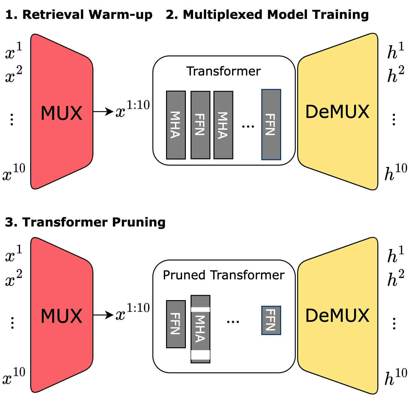
Training a model with PruMUX consists of three phases as shown in Figure 2:

Phase 1: Priming the multiplexed model with the token retrieval objective

We first prime the multiplexed transformer model with a token retrieval task. Murahari et al. (2022) introduced this "retrieval warm-up" self-supervised objective (shown below) and found it to be critical to improve the performance of multiplexed models. $L$ is the length of each input sentence. $I$ is the index of the randomly selected sentence from the input batch.

$$L_{retrieval}(\textbf{x}^{1:N})=\sum_{j=1}^{L}-\log P(\textbf{w}_{j}^{I}|\textbf{h}_{j}^{I})$$

Phase 2: Pre-training and fine-tuning multiplexed models

The multiplexed models from the previous stage are then pre-trained on large-scale text corpora with the masked language modeling (MLM) objective. The pre-trained multiplexed models are then fine-tuned on downstream tasks to yield task-specific multiplexed models.

Phase 3: Model compression

Finally, we use CoFi to jointly prune coarse-grained and fine-grained units in the multiplexed Transformer model. The coarse-grained units include entire attention heads, attention layers, and fully connected layers. The fine-grained units include hidden dimensions and intermediate dimensions of the Transformer model. The demultiplexer’s input dimension is pruned in order to match the pruned hidden dimension of the Transformer model. During the pruning process, CoFi uses knowledge distillation to transfer knowledge from the teacher model, i.e., the task-specific multiplexed model, to the pruned model.

3.2 Implementation Details

We use the pre-trained multiplexed BERT-base models Murahari et al. (2023) with the standard BERT pre-training recipe with the masked language modeling objective for $N=2,5,10$ on Wikipedia Foundation and BooksCorpus Zhu et al. (2015) datasets. We prime the multiplexed model before pre-training with the token-retrieval task in Section 2.2 on the Wikipedia and BooksCorpus datasets. We then train the pre-trained multiplexed models on the four largest GLUE Tasks Wang et al. (2018) – MNLI Williams et al. (2018), QNLI Wang et al. (2018), QQP qqp , and SST-2 Socher et al. (2013). We then use the CoFi structured pruning objective to get pruned multiplexed model on each task dataset. The hyperparameters we use for the training process are shown in Appendix A.1. We perform a single run to train the model for each setting, i.e., task, multiplexer width $N$, model sparsity $s$, following the training process.

3.3 Experiments

(a)

(b)

(c)

(d)

Figure 3: Throughput Improvement ($\times$) of PruMUX (ours), DataMUX Murahari et al. (2023), and CoFi pruning Xia et al. (2022) over the BERT-base model for the MNLI, QNLI, QQP, and SST-2 tasks. The x-axis is the Transformer accuracy, which is inverted to better show throughput improvements of each method for different accuracy loss budgets.

Setup

We would like to answer the question that given an accuracy threshold, whether PruMUX method can achieve a higher throughput than either CoFi or DataMUX alone.

We compare PruMUXed BERT-base model to three baselines:

• BERT-base: BERT-base model trained without data multiplexing and model compression.

• CoFi: BERT-base model pruned by CoFi Xia et al. (2022) with sparsity $s=$ 0.50, 0.60, 0.70, 0.80, 0.90, and 0.95.

• DataMUX: BERT-base model pre-trained by DataMUX Murahari et al. (2023) with the multiplexer width $N=$ 2, 5, and 10.

We have applied PruMUX to the BERT-base model with all combinations of $(N,s)$ for all 4 tasks. We follow the procedure in Xia et al. (2022) to calculate throughput improvements for PruMUXed Transformers and all three baselines, i.e. BERT-base, DataMUX, and CoFi. The evaluation batch size is 128*$N$, where $N$ is the multiplexer width.

Results

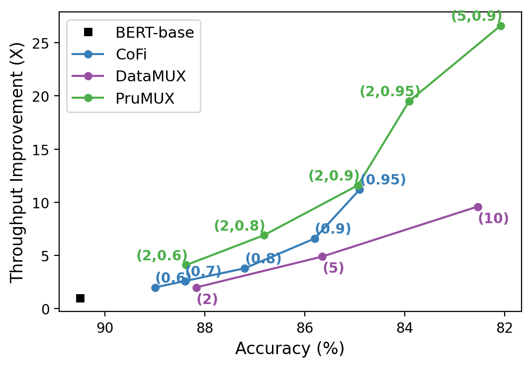
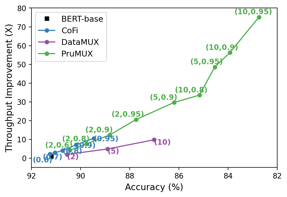
Figure 3 shows the throughput improvements and accuracies of PruMUXed, DataMUXed, and CoFi-Pruned Transformers over the Transformer base model on the MNLI, QNLI, QQP, and SST-2 tasks with all available parameters.

The main takeaway is that PruMUX achieves higher throughput than either CoFi or DataMUX individually in all cases starting at various accuracy thresholds:

• For MNLI, with the accuracy thresholds from 80% to 74%, PruMUX achieves 7.5-29.5X throughput improvement over the BERT-base model, whereas CoFi improves by 4.0-10.6X and DataMUX by 2.0-4.9X.

• For QNLI, with the accuracy thresholds from 87% to 82%, PruMUX achieves 4.1-26.6X improvement, whereas CoFi improves by 3.8-11.2X and DataMUX by 2.0-9.6X.

• For QQP, with the accuracy thresholds from 89% to 86%, PruMUX achieves throughput improvement over BERT-base by 7.6-29.7X, whereas CoFi improves by 10.6X and DataMUX by 2.0-9.8X.

• For SST-2, with the accuracy thresholds from 86.5% to 83%, PruMUX improves the throughput by 10.1-27.8X, whereas CoFi improves by 10.6X and DataMUX by 4.8-9.7X.

The results also confirm the intuition that PruMUX with $(N,s)$ incurs an accuracy loss, loosely speaking, close to the sum of the accuracy loss of DataMUX with $N$ and that of CoFi with $s$. In general, PruMUX can achieve substantial throughput improvement when there is a decent accuracy loss budget.

3.4 Discussion

The results above find top PruMUX performance with all parameter pairs $(N,s)$, where $N=$ 2, 5, 10 and $s=$ 0.60, 0.70, 0.80, 0.90, and 0.95, for each accuracy loss budget. Searching for top PruMUX parameters at a finer parameter granularity will require training and testing on all additional parameter pairs.

Exhaustive tests are impractical. First, for each $N$, pre-training a DataMUX model with multiplexing width $N$ is time-consuming. Second, given each pre-trained model with multiplexer width $N$, different sparsities $s$ provide different throughput and accuracy trade-offs. In order to find the sparsity $s$ with the highest throughput given an accuracy budget, one has to train the model for all possible sparsities. The total training time for the sparsities from 0.60 to 0.95 at the granularity of 0.05 for each $N$ takes over six thousand GPU hours on commodity GPUs, for a small original BERT-base model. A key question is whether one can automatically find a high-throughput ($N,s$) with a small number of PruMUX experiments.

4 Auto-PruMUX

To address the question above, we propose Auto-PruMUX, a method to search for top ($N,s$) parameters, to help practitioners balance the performance vs throughput trade-off.

Our research question is: Suppose we have some experimental data of PruMUX and the experimental data of DataMUX and CoFi, how can we find and predict the top parameters $(N,s)$ given an accuracy loss budget?

Our approach is to develop performance models for the accuracy and throughput of PruMUX. We first train PruMUX models for a set of ($N,s$) combinations and measure both the accuracy and the throughput improvement. We then use this data to fit a throughput model and an accuracy model to predict throughput and accuracy respectively given $(N,s)$ parameters.

We first discuss how we fit the accuracy and throughput models with a set of sparse data points. Given that we are working with a limited set of data points, we opt to use a simple class of interpolation models for modeling PruMUX accuracy and use an estimation model for modeling throughput. We then outline how we leverage these models to predict top $(N,s)$ parameters, given an accuracy loss budget. We then demonstrate the effectiveness of the Auto-PruMUX in predicting the top parameters across a wide range of accuracy loss budgets.

4.1 Task Accuracy Model

We use linear interpolation for our task accuarcy model.

$$\begin{split}&f_{A}(N,s)=\\ &\begin{cases}A_{1,1}(N,s)&\textbf{N}_{0}\leq N\leq\textbf{N}_{1},\textbf{s}_{0}\leq s\leq\textbf{s}_{1},\\ ...\\ A_{i,j}(N,s)&\textbf{N}_{i-1}\leq N\leq\textbf{N}_{i},\textbf{s}_{j-1}\leq s\leq\textbf{s}_{j},\\ ...\\ A_{p,q}(N,s)&\textbf{N}_{p-1}\leq N\leq\textbf{N}_{p},\textbf{s}_{q-1}\leq s\leq\textbf{s}_{q}\\ \end{cases}\end{split}$$

Each term is a linear combination of data multiplexer width and model sparsity.

$$A_{i,j}(N,s)=\sum_{a=0}^{1}\sum_{b=0}^{1}k^{(i,j)}_{ab}N^{a}s^{b}$$

The model is fitted on the gathered data of model task accuracy at different multiplexer width and sparsity.

$$\begin{split}A_{i,j}(\textbf{N}_{i},\textbf{s}_{j})&=Acc(\textbf{N}_{i},\textbf{s}_{j})\\ i&=1,...,p,j=1,...,q\\ \end{split}$$

where N and s are the range of $N$ and $s$ values used to fit the model.

4.2 Throughput Model

We collect the throughput values for all $N$ and $s$ on one task ($task_{0}$) and use the throughput values as the throughput estimations for all tasks.

$$f_{T}(N,s)=Throu_{task_{0}}(N,s)$$

4.3 Predicting $(N,s)$

We use our models, $f_{A}(N,s)$ and $f_{T}(N,s)$, to model the accuracy and the throughput of PruMUX with $N>1$ and $s>0\%$. $Acc(1,s)$ and $Throu(1,s)$ are the measured accuracy and throughput of CoFi-pruned models. $Acc(N,0)$ and $Throu(N,0)$ are the measured accuracy and throughput of DataMUX models. $Acc(1,0)$ and $Throu(1,0)$ are the performance of BERT-base model. We search for $(N,s)$ parameters that maximize $\zeta_{f}$ defined below.

$$\zeta_{f}(N,s)=Throu(N,s)\cdot g(Acc(N,s))$$ (1)

$$g(x)=\begin{cases}1&x\geq\xi\\ 0&x<\xi\\ \end{cases}$$

Intuitively, $\zeta_{f}$ tries to tradeoff task performance and throughput, given an accuracy loss budget $\xi$ with the goal of maximizing the throughput. $g(x)$ provides a mechanism for a strict accuracy threshold - i.e. a model that does not meet the minimum required accuracy will have $\zeta_{f}=0$.

4.4 Experimental Results

Experimental setting

In this section, we show Auto-PruMUX’s prediction results by fitting the performance models using a set of parameter space and predicting top parameters on a larger set of parameter space.

We define the set of ($N,s$) parameter space (test set) as follows.

• BERT-base model - $(N,s)$ $N=$ 1, $s=$ 0.00

• CoFi models - $(N,s)$ $N=$ 1, $\forall s\in$ 0.60, 0.70, 0.80, 0.90, 0.95

• DataMUX models - $(N,s)$ $\forall N\in$ 2,5,10, $s=$ 0.00

• PruMUX models - $(N,s)$ $\forall N\in$ 2,5,10, $\forall s\in$ 0.60, 0.65, 0.70, 0.75, 0.80, 0.85, 0.90, 0.95

We fit the accuracy model with the model accuracies on ($N,s$) $\forall N\in$ 2,5,10, $\forall s\in$ 0.60, 0.70, 0.80, 0.90, 0.95 (training set). We fit the throughput model with the throughput of one task on all parameter pairs.

Our goal is to evaluate the task accuracy model, the throughput model, and parameter prediction performance.

Performance Model Accuracy

To evaluate the accuracy of the task performance models on the training set, we perform leave-one-out cross-validation for each task. We show the fraction $M_{A}$ of accuracy predictions with error falling within $\Delta\xi=1.5\%$ from real accuracy in Table 1. To evaluate the accuracy of the throughput model on the training set, we fit the model using PruMUX’s performance of the QQP task. We show the fraction $M_{T}$ of throughput predictions with error within 20% of real throughput improvement in Table 1. Across different tasks, our accuracy and throughput models are accurate across a broad set of parameter combinations.

Task	$M_{A}$	$M_{T}$	Task	$M_{A}$	$M_{T}$
MNLI	92.3%	92.3%	QQP	100%	100%
QNLI	100%	91.7%	SST-2	100%	100%

Table 1: Accuracy of the task accuracy model ($M_{A}$) and accuracy of the throughput model ($M_{T}$) for PruMUX.

Top Parameter Prediction

We show Auto-PruMUX’s prediction results by fitting the accuracy model on the training set and fitting the throughput model using the throughput of the QQP task, and predicting top parameters on the test set. We show Auto-PruMUX’s top parameter predictions for accuracy loss budget 3% in Table 2. Auto-PruMUX predicts the actual best parameter pairs within its top 3 predictions. In Table 3, we use Auto-PruMUX to predict parameters for accuracy loss budgets in 0%, 0.5%, …, 10% and show the percentage of accuracy loss budgets which Auto-PruMUX predicts the actual best parameter in its top 3 predictions. Auto-PruMUX is able to predict top parameters in most cases.

Task	Auto-PruMUX	Actual Best
	($N,s$), Throu. ($\times$)	($N,s$), Throu. ($\times$)
MNLI	Top 1: (2, 0.65), 4.5$\times$	(2, 0.65), 4.7$\times$
	Top 2: (2, 0.60), 4.2$\times$
	Top 3: (1, 0.80), 4.0$\times$
QNLI	Top 1: (2, 0.70), 5.0$\times$	(2, 0.65), 4.5$\times$
	Top 2: (2, 0.65), 4.2$\times$
	Top 3: (2, 0.60), 3.9$\times$
QQP	Top 1: (2, 0.90), 12.4$\times$	(2, 0.90), 12.4$\times$
	Top 2: (5, 0.65), 10.6$\times$
	Top 3: (1, 0.95), 10.6$\times$
SST-2	Top 1: (1, 0.95), 10.6$\times$	(1, 0.95), 10.6$\times$
	Top 2: (1, 0.90), 6.2$\times$
	Top 3: (2, 0.70), 5.0$\times$

Table 2: Auto-PruMUX top 3 $(N,s)$ predictions for different tasks with accuracy loss budgets of 3% along with their predicted throughput improvements. The actual best parameters $(N,s)$ and their throughput improvements are shown in the last column.

Task	Accuracy	Task	Accuracy
MNLI	81.0%	QQP	100%
QNLI	90.5%	SST-2	90.5%

Table 3: Percentage of accuracy loss budgets in 0%, 0.5%, …, 9.5%, 10% which Auto-PruMUX predicts the actual best ($N,s$) parameter in its top 3 predictions.

5 Related Work

Model Compression

Model compression reduces the number of model parameters with minimal loss in task performance. A well-studied method is network pruning, which removes unimportant connections from a network with minimal or no accuracy loss LeCun et al. (1989); Hanson and Pratt (1989); Hassibi et al. (1993).

Unstructured pruning Han et al. (2015b, a); Zhu and Gupta (2017); Frankle and Carbin (2019); Chen et al. (2020a); Huang et al. (2021); Sanh et al. (2020) does not impose any constraints on the locations of non-zero weights. The resulting network can achieve high sparsity but may not run efficiently on common hardware such as GPUs.

Structured pruning produces structured sparse matrices that can take better advantage of the parallelism in existing hardware, but its sparsity is relatively lower than the unstructured pruning method for the same accuracy loss budget Yu et al. (2017); Narang et al. (2017); Wen et al. (2017); Mao et al. (2017); Wang et al. (2019); McDanel et al. (2022). Structured pruning has been applied to transformers to improve inference throughput Fan et al. (2019); Sajjad et al. (2023); Voita et al. (2019); Michel et al. (2019); Prasanna et al. (2020); Chen et al. (2020b); McCarley et al. (2019); Hou et al. (2020); Yao et al. (2021).

Distillation compresses a model by transferring knowledge from a large teacher model to a small student model Hinton et al. (2015). General distillation for Transformer models learn from unlabeled corpus Sanh et al. (2019); Sun et al. (2020); Wang et al. (2020); Turc et al. (2019); Jiao et al. (2019). Task-specific distillation for Transformer models learns on task-specific data Sun et al. (2019). Jiao et al. (2019) combines the two distillation methods to improve performance.

Pruning with distillation objective have been explored Sanh et al. (2020); Lagunas et al. (2021). Xia et al. (2022) proposes structured pruning with distillation objective to reduce the Transformer parameters by up to 95% and achieve over 10x speedups with small accuracy drops.

Multi-input Multi-output Models

Multi-input Multi-output models concurrently process multiple inputs within one neural network to reduce network over-parameterization. Havasi et al. (2021) and Ramé et al. (2021) train independent sub-networks and ensemble them into a multi-input multi-output model to obtain better accuracy and uncertainty estimation with inference cost similar to a single network. Murahari et al. (2022) proposes data multiplexing technique to multiplex multiple input sequences into one input sequence to Transformer model, which leads to up to 18x inference speedup. Murahari et al. (2023) develops pre-trained multiplexed language models to improve model throughput.

Performance Modeling

Various methods have been proposed to estimate the performance of machine learning models. Justus et al. (2018) proposes a method to predict CNN execution time for training. They decompose CNN training into several components, estimate the time for each component, and predict the model execution time as the combination of different components. Qi et al. (2017); Cai et al. (2017) predict the performance of deep neural networks based on the neural network models’ architecture. Stamoulis et al. (2018) proposes predictive models for the power and memory of neural networks executing on GPUs. Machine-learning-based cost models Chen et al. (2018); Bouzidi et al. (2020) have been explored to predict program running time.

Interpolation Davis (1975) is widely used in engineering and science Oliver and Webster (1990); Keys (1981); Lehmann et al. (1999), where function values at discrete data points are collected in experiments and the function values at the intervals between discrete data points are estimated using interpolation methods.

6 Conclusion

We propose PruMUX, a method to combine model compression and data multiplexing to build high throughput transformers. Our implementation of PruMUX makes use of CoFi and DataMUX and we show that it achieves substantial throughput improvement over either CoFi or DataMUX for a large range of accuracy thresholds.

We conclude that the reason that PruMUX performs well in certain range of accuracy loss budgets is that CoFi and DataMUX improve the throughput of a model in two different dimensions: reducing the latency of an inference and compressing multiple inferences. When the accuracy loss budget is large, both methods lead to non-linear drops in model accuracy, PruMUX can achieve much better performance than either approach because it uses more conservative parameters for CoFi and DataMUX before each reaches its bad trade-off point.

We also present Auto-PruMUX, a meta-model to automatically predict high-performance parameter combinations for a desired accuracy on a task. We show it is promising in predicting parameters without individual data points and additional training.

7 Limitations

Our experiments are limited to 3 DataMUXed pre-trained models ($N=$ 2, 5, and 10) due to compute constraints. More pre-trained models with different $N$’s would provide PruMUX with more options to improve throughput and would allow us to conduct a more detailed evaluation of Auto-PruMUX.

PruMUX uses CoFi as its model compression method. Experiments with other methods could improve our understanding of the interactions between model compression and data multiplexing.

8 Acknowledgement

Karthik Narasimhan and Vishvak Murahari gratefully acknowledge support from the Samsung GRO program.

Appendix A Appendix

A.1 Hyperparameters for Model Training

Table 4 and Table 5 show the hyperparameters used in CoFi training and PruMUX training correspondingly. The hyperparameters are from CoFi’s open-sourced code.

Hyperparamter	CoFi
distill layer loss alpha	0.9, 0.7, 0.5
distill ce loss alpha	0.1, 0.3, 0.5
layer distill version	3, 4, 6
sparsity epsilon	0.01
max seq length	128
pruning batch size	32
finetune batch size	64
training epoch	20
finetune epoch	20
distill temp	2
scheduler type	linear
prepruning finetune epoch	1
lagrangian warmup epoch	2
pruning learning rate	2e-5
finetune learning rate	1e-5, 2e-5, 3e-5

Table 4: Hyperparameters in CoFi training

Hyperparamter	PruMUX
distill layer loss alpha	0.9, 0.7, 0.5
distill ce loss alpha	0.1, 0.3, 0.5
layer distill version	3, 4, 6
sparsity epsilon	0.01
max seq length	128
pruning batch size	32*N
finetune batch size	64
training epoch	40
finetune epoch	40
distill temp	2
scheduler type	linear
prepruning finetune epoch	0
lagrangian warmup epoch	2
pruning learning rate	5e-5
finetune learning rate	1e-5, 2e-5
	3e-5, 5e-5

Table 5: Hyperparameters in PruMUX training

A.2 Dataset Statistics

Table 6 shows the sizes and metrics of the datasets in our experiments.

Task	Train Size	Metric
MNLI	393k	accuracy
QNLI	105k	accuracy
QQP	364k	accuracy
SST-2	67k	accuracy

Table 6: Data statistics of GLUE datasets

A.3 Potential Risks

Multiplexing with model compression may lead to information leakage between different instances, which can potentially raise privacy concerns if used in a public API serving these models.

References

- (1) Quora. data.quora.com/First-Quora-Dataset-Release-Question-Pairs. Accessed: 2022-10-15.
- Allen-Zhu et al. (2019) Zeyuan Allen-Zhu, Yuanzhi Li, and Zhao Song. 2019. A convergence theory for deep learning via over-parameterization. In International Conference on Machine Learning, pages 242–252. PMLR.
- Bouzidi et al. (2020) Halima Bouzidi, Hamza Ouarnoughi, Smail Niar, and Abdessamad Ait El Cadi. 2020. Performance prediction for convolutional neural networks in edge devices. arXiv preprint arXiv:2010.11297.
- Cai et al. (2017) Ermao Cai, Da-Cheng Juan, Dimitrios Stamoulis, and Diana Marculescu. 2017. Neuralpower: Predict and deploy energy-efficient convolutional neural networks. In Asian Conference on Machine Learning, pages 622–637. PMLR.
- Chen et al. (2020a) Tianlong Chen, Jonathan Frankle, Shiyu Chang, Sijia Liu, Yang Zhang, Zhangyang Wang, and Michael Carbin. 2020a. The lottery ticket hypothesis for pre-trained bert networks. Advances in neural information processing systems, 33:15834–15846.
- Chen et al. (2018) Tianqi Chen, Thierry Moreau, Ziheng Jiang, Lianmin Zheng, Eddie Yan, Meghan Cowan, Haichen Shen, Leyuan Wang, Yuwei Hu, Luis Ceze, et al. 2018. Tvm: An automated end-to-end optimizing compiler for deep learning. arXiv preprint arXiv:1802.04799.
- Chen et al. (2020b) Xiaohan Chen, Yu Cheng, Shuohang Wang, Zhe Gan, Zhangyang Wang, and Jingjing Liu. 2020b. Earlybert: Efficient bert training via early-bird lottery tickets. arXiv preprint arXiv:2101.00063.
- Davis (1975) Philip J Davis. 1975. Interpolation and approximation. Courier Corporation.
- Devlin et al. (2018) Jacob Devlin, Ming-Wei Chang, Kenton Lee, and Kristina Toutanova. 2018. Bert: Pre-training of deep bidirectional transformers for language understanding. arXiv preprint arXiv:1810.04805.
- Fan et al. (2019) Angela Fan, Edouard Grave, and Armand Joulin. 2019. Reducing transformer depth on demand with structured dropout. arXiv preprint arXiv:1909.11556.
- (11) Wikimedia Foundation. Wikimedia downloads.
- Frankle and Carbin (2019) Jonathan Frankle and Michael Carbin. 2019. The lottery ticket hypothesis: Finding sparse, trainable neural networks. In International Conference on Learning Representations.
- Han et al. (2015a) Song Han, Huizi Mao, and William J Dally. 2015a. Deep compression: Compressing deep neural networks with pruning, trained quantization and huffman coding. arXiv preprint arXiv:1510.00149.
- Han et al. (2016) Song Han, Huizi Mao, and William J. Dally. 2016. Deep compression: Compressing deep neural networks with pruning, trained quantization and huffman coding. In International Conference on Learning Representations.
- Han et al. (2015b) Song Han, Jeff Pool, John Tran, and William J. Dally. 2015b. Learning both weights and connections for efficient neural networks. In Advances in neural information processing systems, pages 1135–1143.
- Hanson and Pratt (1989) Stephen Jose Hanson and Lorien Y Pratt. 1989. Comparing biases for minimal network construction with back-propagation. In Advances in neural information processing systems, page 177–185.
- Hassibi et al. (1993) Babak Hassibi, David G Stork, and Gregory J Wolff. 1993. Optimal brain surgeon and general network pruning. In IEEE international conference on neural networks, pages 293–299. IEEE.
- Havasi et al. (2021) Marton Havasi, Rodolphe Jenatton, Stanislav Fort, Jeremiah Zhe Liu, Jasper Snoek, Balaji Lakshminarayanan, Andrew Mingbo Dai, and Dustin Tran. 2021. Training independent subnetworks for robust prediction. In International Conference on Learning Representations.
- Hinton et al. (2015) Geoffrey Hinton, Oriol Vinyals, Jeff Dean, et al. 2015. Distilling the knowledge in a neural network. arXiv preprint arXiv:1503.02531, 2(7).
- Hou et al. (2020) Lu Hou, Zhiqi Huang, Lifeng Shang, Xin Jiang, Xiao Chen, and Qun Liu. 2020. Dynabert: Dynamic bert with adaptive width and depth. Advances in Neural Information Processing Systems, 33:9782–9793.
- Huang et al. (2021) Shaoyi Huang, Dongkuan Xu, Ian EH Yen, Sung-en Chang, Bingbing Li, Shiyang Chen, Mimi Xie, Hang Liu, and Caiwen Ding. 2021. Sparse progressive distillation: Resolving overfitting under pretrain-and-finetune paradigm. arXiv preprint arXiv:2110.08190.
- Jiao et al. (2019) Xiaoqi Jiao, Yichun Yin, Lifeng Shang, Xin Jiang, Xiao Chen, Linlin Li, Fang Wang, and Qun Liu. 2019. Tinybert: Distilling bert for natural language understanding. arXiv preprint arXiv:1909.10351.
- Justus et al. (2018) Daniel Justus, John Brennan, Stephen Bonner, and Andrew Stephen McGough. 2018. Predicting the computational cost of deep learning models. In 2018 IEEE international conference on big data (Big Data), pages 3873–3882. IEEE.
- Keys (1981) Robert Keys. 1981. Cubic convolution interpolation for digital image processing. IEEE transactions on acoustics, speech, and signal processing, 29(6):1153–1160.
- Lagunas et al. (2021) François Lagunas, Ella Charlaix, Victor Sanh, and Alexander M Rush. 2021. Block pruning for faster transformers. arXiv preprint arXiv:2109.04838.
- LeCun et al. (1989) Yann LeCun, John S Denker, and Sara A Solla. 1989. Optimal brain damage. In Advances in neural information processing systems, pages 598–605.
- Lehmann et al. (1999) T.M. Lehmann, C. Gonner, and K. Spitzer. 1999. Survey: interpolation methods in medical image processing. IEEE Transactions on Medical Imaging, 18(11):1049–1075.
- Mao et al. (2017) Huizi Mao, Song Han, Jeff Pool, Wenshuo Li, Xingyu Liu, Yu Wang, and William J Dally. 2017. Exploring the regularity of sparse structure in convolutional neural networks. arXiv preprint arXiv:1705.08922.
- McCarley et al. (2019) JS McCarley, Rishav Chakravarti, and Avirup Sil. 2019. Structured pruning of a bert-based question answering model. arXiv preprint arXiv:1910.06360.
- McDanel et al. (2022) Bradley McDanel, Helia Dinh, and John Magallanes. 2022. Accelerating dnn training with structured data gradient pruning. arXiv preprint arXiv:2202.00774.
- Michel et al. (2019) Paul Michel, Omer Levy, and Graham Neubig. 2019. Are sixteen heads really better than one? Advances in neural information processing systems, 32.
- Murahari et al. (2023) Vishvak Murahari, Ameet Deshpande, Carlos E Jimenez, Izhak Shafran, Mingqiu Wang, Yuan Cao, and Karthik Narasimhan. 2023. Mux-plms: Pre-training language models with data multiplexing. arXiv preprint arXiv:2302.12441.
- Murahari et al. (2022) Vishvak Murahari, Carlos E Jimenez, Runzhe Yang, and Karthik R Narasimhan. 2022. DataMUX: Data multiplexing for neural networks. In Thirty-Sixth Conference on Neural Information Processing Systems.
- Narang et al. (2017) Sharan Narang, Eric Undersander, and Gregory Diamos. 2017. Block-sparse recurrent neural networks. arXiv preprint arXiv:1711.02782.
- Oliver and Webster (1990) Margaret A Oliver and Richard Webster. 1990. Kriging: a method of interpolation for geographical information systems. International Journal of Geographical Information System, 4(3):313–332.
- Prasanna et al. (2020) Sai Prasanna, Anna Rogers, and Anna Rumshisky. 2020. When bert plays the lottery, all tickets are winning. arXiv preprint arXiv:2005.00561.
- Qi et al. (2017) Hang Qi, Evan R Sparks, and Ameet Talwalkar. 2017. Paleo: A performance model for deep neural networks. In International Conference on Learning Representations.
- Radhakrishnan et al. (2020) Adityanarayanan Radhakrishnan, Mikhail Belkin, and Caroline Uhler. 2020. Overparameterized neural networks implement associative memory. Proceedings of the National Academy of Sciences, 117(44):27162–27170.
- Ramé et al. (2021) Alexandre Ramé, Rémy Sun, and Matthieu Cord. 2021. Mixmo: Mixing multiple inputs for multiple outputs via deep subnetworks. In Proceedings of the IEEE/CVF International Conference on Computer Vision (ICCV).
- Sajjad et al. (2023) Hassan Sajjad, Fahim Dalvi, Nadir Durrani, and Preslav Nakov. 2023. On the effect of dropping layers of pre-trained transformer models. Computer Speech & Language, 77:101429.
- Sanh et al. (2019) Victor Sanh, Lysandre Debut, Julien Chaumond, and Thomas Wolf. 2019. Distilbert, a distilled version of bert: smaller, faster, cheaper and lighter. arXiv preprint arXiv:1910.01108.
- Sanh et al. (2020) Victor Sanh, Thomas Wolf, and Alexander Rush. 2020. Movement pruning: Adaptive sparsity by fine-tuning. Advances in Neural Information Processing Systems, 33:20378–20389.
- Socher et al. (2013) Richard Socher, Alex Perelygin, Jean Wu, Jason Chuang, Christopher D Manning, Andrew Y Ng, and Christopher Potts. 2013. Recursive deep models for semantic compositionality over a sentiment treebank. In Proceedings of the 2013 conference on empirical methods in natural language processing, pages 1631–1642.
- Stamoulis et al. (2018) Dimitrios Stamoulis, Ermao Cai, Da-Cheng Juan, and Diana Marculescu. 2018. Hyperpower: Power-and memory-constrained hyper-parameter optimization for neural networks. In 2018 Design, Automation & Test in Europe Conference & Exhibition (DATE), pages 19–24. IEEE.
- Sun et al. (2019) Siqi Sun, Yu Cheng, Zhe Gan, and Jingjing Liu. 2019. Patient knowledge distillation for bert model compression. arXiv preprint arXiv:1908.09355.
- Sun et al. (2020) Zhiqing Sun, Hongkun Yu, Xiaodan Song, Renjie Liu, Yiming Yang, and Denny Zhou. 2020. Mobilebert: a compact task-agnostic bert for resource-limited devices. arXiv preprint arXiv:2004.02984.
- Turc et al. (2019) Iulia Turc, Ming-Wei Chang, Kenton Lee, and Kristina Toutanova. 2019. Well-read students learn better: On the importance of pre-training compact models. arXiv preprint arXiv:1908.08962.
- Voita et al. (2019) Elena Voita, David Talbot, Fedor Moiseev, Rico Sennrich, and Ivan Titov. 2019. Analyzing multi-head self-attention: Specialized heads do the heavy lifting, the rest can be pruned. arXiv preprint arXiv:1905.09418.
- Wang et al. (2018) Alex Wang, Amanpreet Singh, Julian Michael, Felix Hill, Omer Levy, and Samuel R Bowman. 2018. Glue: A multi-task benchmark and analysis platform for natural language understanding. arXiv preprint arXiv:1804.07461.
- Wang et al. (2020) Wenhui Wang, Furu Wei, Li Dong, Hangbo Bao, Nan Yang, and Ming Zhou. 2020. Minilm: Deep self-attention distillation for task-agnostic compression of pre-trained transformers. Advances in Neural Information Processing Systems, 33:5776–5788.
- Wang et al. (2019) Ziheng Wang, Jeremy Wohlwend, and Tao Lei. 2019. Structured pruning of large language models. arXiv preprint arXiv:1910.04732.
- Wen et al. (2017) Wei Wen, Yuxiong He, Samyam Rajbhandari, Minjia Zhang, Wenhan Wang, Fang Liu, Bin Hu, Yiran Chen, and Hai Li. 2017. Learning intrinsic sparse structures within long short-term memory. arXiv preprint arXiv:1709.05027.
- Williams et al. (2017) Adina Williams, Nikita Nangia, and Samuel R Bowman. 2017. A broad-coverage challenge corpus for sentence understanding through inference. arXiv preprint arXiv:1704.05426.
- Williams et al. (2018) Adina Williams, Nikita Nangia, and Samuel R Bowman. 2018. A broad-coverage challenge corpus for sentence understanding through inference. In NAACL-HLT.
- Xia et al. (2022) Mengzhou Xia, Zexuan Zhong, and Danqi Chen. 2022. Structured pruning learns compact and accurate models. In Proceedings of the 60th Annual Meeting of the Association for Computational Linguistics (Volume 1: Long Papers), pages 1513–1528, Dublin, Ireland. Association for Computational Linguistics.
- Yao et al. (2021) Zhewei Yao, Linjian Ma, Sheng Shen, Kurt Keutzer, and Michael W Mahoney. 2021. Mlpruning: A multilevel structured pruning framework for transformer-based models. arXiv preprint arXiv:2105.14636.
- Yu et al. (2017) Jiecao Yu, Andrew Lukefahr, David Palframan, Ganesh Dasika, Reetuparna Das, and Scott Mahlke. 2017. Scalpel: Customizing dnn pruning to the underlying hardware parallelism. ACM SIGARCH Computer Architecture News, 45(2):548–560.
- Zhu and Gupta (2017) Michael Zhu and Suyog Gupta. 2017. To prune, or not to prune: exploring the efficacy of pruning for model compression. arXiv preprint arXiv:1710.01878.
- Zhu et al. (2015) Yukun Zhu, Ryan Kiros, Rich Zemel, Ruslan Salakhutdinov, Raquel Urtasun, Antonio Torralba, and Sanja Fidler. 2015. Aligning books and movies: Towards story-like visual explanations by watching movies and reading books. In The IEEE International Conference on Computer Vision (ICCV).