Under-Parameterized Double Descent for Ridge Regularized Least Squares Denoising of Data on a Line

Abstract

The relationship between the number of training data points, the number of parameters in a statistical model, and the generalization capabilities of the model has been widely studied. Previous work has shown that double descent can occur in the over-parameterized regime, and believe that the standard bias-variance trade-off holds in the under-parameterized regime. In this paper, we present a simple example that provably exhibits double descent in the under-parameterized regime. For simplicity, we look at the ridge regularized least squares denoising problem with data on a line embedded in high-dimension space. By deriving an asymptotically accurate formula for the generalization error, we observe sample-wise and parameter-wise double descent with the peak in the under-parameterized regime rather than at the interpolation point or in the over-parameterized regime.

Further, the peak of the sample-wise double descent curve corresponds to a peak in the curve for the norm of the estimator, and adjusting $\mu$, the strength of the ridge regularization, shifts the location of the peak. We observe that parameter-wise double descent occurs for this model for small $\mu$. For larger values of $\mu$, we observe that the curve for the norm of the estimator has a peak but that this no longer translates to a peak in the generalization error. Moreover, we study the training error for this problem. The considered problem setup allows for studying the interaction between two regularizers. We provide empirical evidence that the model implicitly favors using the ridge regularizer over the input data noise regularizer. Thus, we show that even though both regularizers regularize the same quantity, i.e., the norm of the estimator, they are not equivalent.

1 Introduction

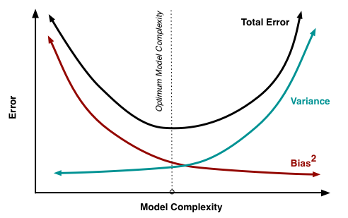
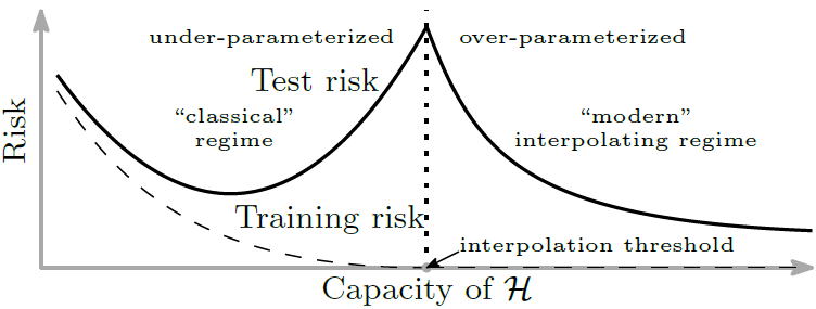
This paper aims to demonstrate interesting new phenomena that suggest that our understanding of the relationship between the number of data points, the number of parameters, and the generalization error is incomplete, even for simple linear models with data on a line. The classical bias-variance theory postulates that the generalization risk versus the number of parameters for a fixed number of training data points is U-shaped (Figure LABEL:fig:bias-variance). However, modern machine learning showed that if we keep increasing the number of parameters, the generalization error eventually starts decreasing again [1, 2] (Figure LABEL:fig:doubledescent). This second descent has been termed as double descent and occurs in the over-parameterized regime, that is when the number of parameters exceeds the number of data points. Understanding the location and the cause of such peaks in the generalization error is of significant importance. Hence many recent works have theoretically studied the generalization error for linear regression [3, 5, 6, 7, 8, 9, 10, 11, 12, 4] and kernelized regression [13, 14, 15, 16, 17, 18, 19, 20, 21] and show that there exists a peak at the boundary between the under and over-parameterized regimes. Further works such as [22, 10, 23, 24, 25] show that there can be multiple descents in the over-parameterized regime and [26] shows that any shaped generalization error curve can occur in the over-parameterized regime. However, all prior works assume that the classical bias-variance trade-off is true in the under-parameterized regime.

(a)

(b)

Figure 1: Classical bias-variance trade-off and modern double descent.

The implicit bias of the learning algorithm is a possible reason that the error decreases in the over-parameterized regime [28, 29, 30, 31, 32, 33]. In the under-parameterized regime, there is exactly one solution that minimizes the loss. However, once in the over-parameterized regime, there are many different solutions, and the training algorithm implicitly picks one that generalizes well. For linear models, the generalization error and the variance are very closely related to the norm of the estimator [11, 34]. Then, using the well-known fact that the pseudo-inverse solution to the least squares problem is the minimum norm solution, we see that the training algorithm picks solutions with the minimum norm. Hence this learning algorithm minimizes the variance and lowers the generalization error.

Double descent can be mitigated by optimally tuning the model’s regularization [24, 34, 35]. There are two different phenomena in the literature. First, the optimal amount of regularization is independent of the number of training data points [24]. Second, the optimal regularization follows a double descent curve with respect to the number of training data points, with the peak occurring at the same spot as the peak in the generalization error curve [34, 36]. Further, increasing the amount of regularization from zero to the optimal amount of regularization results in the magnitude of the peak in the generalization getting smaller until a peak no longer exists. However, the location of the peak does not change by changing the amount of regularization.

In contrast with prior work, this paper shows that double descent can occur in the under-parameterized regime. Specifically, when denoising data on a line embedded in high-dimensional space using a denoiser obtained as the pseudo-inverse solution for the ridge regularized least squares problem, we show that a peak in the generalization error curve occurs in the under-parameterized regime. We also show that changing the ridge regularization strength changes the location of the peak. To further understand the location of the peak, we derive the exact asymptotics for the training error and explore the connections between the norm of the estimator and the peak of the generalization error curve. Moreover, since this model has two regularizers, we study the trade-off between them and notice that they are not equivalent.

Main Contributions.

The major contributions of this paper are as follows.

• (Generalization error) We derive a theoretical formula for the generalization error (Theorem 1).

• (Under-parameterized double descent) We prove (Theorem 2) and empirically demonstrate that the generalization error versus the number of data points curve has double descent in the under-parameterized regime. For small values of the ridge regularization coefficient $\mu$, we empirically show that the generalization error versus the number of parameters curve exhibits double descent in the under-parameterized regime.

• (Location of the peak) The peak location depends on the regularization strength. We provide evidence (Theorem 3) that the peak is near $c=\frac{1}{\mu^{2}+1}$ for the sample-wise double descent curves.

• (Norm of the estimator) We show that the peak in the curve for the generalization error versus the number of training data points corresponds to a peak in the norm of the estimator. However, versus the number of parameters, we show that there is still a peak in the curve for the norm of the estimator (Theorem 4), but this no longer corresponds to a peak in the generalization error.

• (Training Error) We derive an asymptotically exact formula for the training error in the under-parameterized regime (Theorem 5). We notice a weak correlation between the location of the double descent peak and a local minimum of the third derivative of the training error.

• (Regularization Trade-off) We explore the trade-offs between the two regularizers and the generalization error. The model’s implicit bias leads to the best generalization error occurring with high data quality (low noise regularization) and high ridge regularization. Thus, showing that the two regularizers have very different roles in relation to the generalization error (Section 4).

Low-Dimensional Data.

It is important to highlight that using low-rank data does not immediately imply that a peak occurs in the under-parameterized regime. Specifically, [37] looks at the problem of Principal Component Regression (PCR), which is a procedure that projects data onto the space spanned by the first $k$ principal components. Note that the data lives in a low-dimensional space embedded in a higher dimensional space. They show that projecting onto low-dimensional versions of the data acts as a regularizer and removes the peak altogether. [37] also study the problem with data poisoning, i.e., adding one outlier to the training data, and show that things can be arbitrarily bad in the over-parameterized regime. [38], also looks at a similar problem, but they consider isotropic Gaussian data and project onto the first $k$ components. In this case, the data is artificially high-dimensional (since only the first $k$ coordinates are non-zero). They again see a peak at the interpolation point ($N_{trn}=k$). [39] also looks at a version of PCR in which the data dimension is reduced. That is, the data is not embedded in high-dimensional space anymore. [39] sees a peak at the boundary between the under and over-parameterized regions. Finally, [34, 40] look at the denoising problem for low-dimensional data and have peaks at $c=1$. Hence, low-dimensional data does not immediately imply a peak in the under-parameterized regime. Table 1 compares common assumptions and the location of the peak.

Table 1: Table showing various assumptions on the data and the location of the double descent peak for linear regression and denoising. We only present a subset of references for each problem setting.

Noise	Ridge Reg.	Dimension	Peak Location	Reference
Input	Yes	1	Under-parameterized	This paper.
Input	No	Low	Over-parameterized/interpolation point	[34, 40]
Output	No	Full	Over-parameterized/interpolation point	[8, 5, 11]
Output	Yes	Full	Over-parameterized/interpolation point	[24, 11]
Output	No	Low	Over-parameterized/interpolation point	[38]
Output	Yes	Low	Over-parameterized/interpolation point	[39]
Output	No	Low	No peak	[37]

Other Related Works.

Much work has been done on understanding the implicit bias for gradient-based methods and linear models [41, 45, 46, 47, 48, 49, 50, 51, 52, 42, 43, 44]. Significant work has also been done to understand the role of noise as a regularizer and its impact on generalization [53, 54, 55, 56, 57, 58, 34]. Other related works include the use of noise to learn features [59, 60, 61, 62], to improve robustness [63, 64, 65], to prevent adversarial attacks [66, 67], and the connection to training dynamics [68]. There has also been work to understand Bayes optimal denoiser using matrix factorization [69, 70, 71, 72, 73]. Finally, works such as [39, 74, 34, 24, 35] have looked at theoretically determining the optimal regularization strength.

Structure and Limitations.

The rest of this paper is organized as follows. Section 2 provides basic definitions and modeling assumptions. One of the major differences between prior work and this work is the shifting of the noise from the output variable to the input variable. Section 2.1 details the equivalent model with output noise. The model in Section 2.1 serves as a baseline for previously seen phenomena and will be used to contrast the phenomena seen here. Section 3 provides the theoretical results that show that the peak occurs in the under-parameterized regime. The section also explores why the peak occurs where it does and empirically verifies the results. Finally, Section 4 explores the trade-off between the two regularizers.

We highlight some limitations of our work. Our analysis is very much for the ridge regularized least squares linear denoising problem, and significant work would be required to adapt any of the results for neural networks or other linear methods with real data.

2 Background and Model Assumptions

We provide some crucial definitions needed for this paper. Throughout the paper, we assume that noiseless training data $x_{i}$ live in $\mathbb{R}^{d}$ and that we have access to a $d\times N_{trn}$ matrix $X_{trn}$ of training data. We then solve a least squares problem with linear models, such as linear regression or denoising. Then given new data $X_{tst}\in\mathbb{R}^{d\times N_{tst}}$, we are interested in the least squares generalization error. Two scenarios for the generalization error curve are considered; data scaling and parameter scaling.

Definition 1.

• Data scaling refers to the regime in which we fix the dimension $d$ of the input data and vary the number of training data points $N_{trn}$. This is also known as the sample-wise regime.

• Parameter scaling refers to the regime in which we fix the number of training data points $N_{trn}$ and vary the dimension $d$ of the input data. This is also known as the parameter-wise regime.

Definition 2.

• A linear model is under-parameterized, if $d<N_{trn}$.

• A linear model is over-parameterized, if $d>N_{trn}$.

• The boundary of the under and over-parameterized regimes is when $d=N_{trn}$.

• Given $N_{trn}$, the interpolation point is the smallest $d$ for the which the model has zero training error.

• A curve has double descent if the curve has a local maximum or peak.

• The aspect ratio of an $m\times n$ matrix is $c:=m/n$.

Note that double descent originally referred to curves that initially decreased, then increased, and then decreased again. However, this is not the case in subsequent literature, as for many linear models, the first descent is not seen. Instead, an initial ascent followed by a descent is observed. Since the presence of a peak and the subsequent descent are the crucial aspects of interest, we shall refer to a curve with a local maximum as exhibiting double descent.

2.1 Prior Double Descent

This section presents a baseline model from prior work on double descent. This is to highlight prior important phenomena related to double descent in the literature. Concretely, consider the following simple linear model that is a special case of the general models studied in [5, 11, 8, 24] amongst many other works. Let $x_{i}\sim\mathcal{N}(0,I_{d})$ and let $\beta\in\mathbb{R}^{d}$ be a linear model with $\|\beta\|=1$. Let $y_{i}=\beta^{T}x_{i}+\xi_{i}$ where $\xi\sim\mathcal{N}(0,1)$. Then, let

$$\beta_{opt}:=\operatorname*{arg\,min}_{\tilde{\beta}}\|\beta^{T}X_{trn}-\tilde{\beta}X_{trn}+\xi_{trn}\|$$

where $\xi_{trn}\in\mathbb{R}^{N_{trn}\times 1}$. Then the excess risk, when taking the expectation over the new test data point, can be expressed as

$$\mathcal{R}=\|\beta-\beta_{opt}\|^{2}=\|\beta\|^{2}+\|\beta_{opt}\|^{2}-2\beta^{T}\beta_{opt}.$$

Let $c$ be the aspect ratio of the data matrix. That is, $c=d/N_{trn}$. Then it can be shown that

$$\mathbb{E}_{X_{trn},\xi_{trn}}[\|\beta_{opt}\|^{2}]=\begin{cases}1+\frac{c}{1-c}&c<1\\ \frac{1}{c}+\frac{1}{c-1}&c>1\end{cases}\quad\text{ and }\quad\mathbb{E}_{X_{trn},\xi_{trn}}[\beta^{T}\beta_{opt}]=\begin{cases}1&c<1\\ \frac{1}{c}&c>1\end{cases}$$

Then, the excess risk can be expressed as $\displaystyle\mathcal{R}=\begin{cases}\frac{c}{1-c}&c<1\\ \frac{c-1}{c}+\frac{1}{c-1}&c>1\end{cases}.$

There are a few important features that are considered staple in many prior double descent curves for linear models that are present in this model.

1. The peak happens at $c=1$, on the border between the under and over-parameterized regimes.

2. Further, at $c=1$ the training error equals zero. Hence this is the interpolation point.

3. The peak occurs due to the expected norm of the estimator $\beta_{opt}$ blowing up near the interpolation point.

Further, [26] proved that double descent cannot take place in the under-parameterized regime for the above model.

For the ridge regularized version of the regression problem, as shown in [24, 11], the peak is always at $c=1$ (see Figure 1 in [24]). Further, as seen in Figure 1 in [24], changing the strength of the regularization changes the magnitude of the peak. Not the location of the peak.

Building on this, [23] looks at the model where $y_{i}=f(x_{i})+\xi_{i}$ and shows that triple descent occurs for the random features model [75] in the over-parameterized regime. Specifically, as before, they show that the first peak is due to the norm of the estimator peaking, and that the second peak is due to the initialization of the random features. Their results, Figure 3 in [23], show that the peaks only occur if the model is over-parameterized. Further [26] shows that by considering a variety of product data distributions, any shaped risk curve can be observed in the over-parameterized regime.

2.2 Assumptions for Denoising Model

With the context from the previous section in mind, we are now ready to present the assumptions for the input noise model with double descent in the under-parameterized regime. Here we build on [34], in which they switch focus from looking at noise on the outputs to noise on the inputs. For the denoising problem, let $A_{trn}\in\mathbb{R}^{d\times N_{trn}}$ be the noise matrix, then the ridge regularized least square denoiser $W_{opt}$ is the minimum norm solution to

$$W_{opt}:=\operatorname*{arg\,min}_{W}\|X_{trn}-W(X_{trn}+A_{trn})\|_{F}^{2}+\mu^{2}\|W\|_{F}^{2}.$$ (1)

Given test data $X_{tst}$, the mean squared generalization error is given by

$$\mathcal{R}(W_{opt})=\mathbb{E}_{A_{trn},A_{tst}}\left[\frac{1}{N_{tst}}\|X_{tst}-W_{opt}(X_{tst}+A_{tst})\|_{F}^{2}\right].$$ (2)

Remark 1 (Linear Model).

The reason we consider linear models with the pseudo-inverse solution is that this eliminates other factors, such as the initialization of the network that could be a cause of the double descent [23].

Assumptions for the data.

We assume that the data lies on a line embedded in high-dimensional space. We note that [40] could be used to extend the analysis to the rank $r$ case.

Assumption 1.

Let $\mathcal{U}\subset\mathbb{R}^{d}$ be a one dimensional space with a unit basis vector $u$. Then let $X_{trn}=\sigma_{trn}uv_{trn}^{T}\in\mathbb{R}^{d\times N_{trn}}$ and $X_{tst}=\sigma_{tst}uv_{tst}^{T}\in\mathbb{R}^{d\times N_{tst}}$ be the respective SVDs for the training data and test data matrices. We further assume that $\sigma_{trn}=O(\sqrt{N_{trn}})$ and $\sigma_{tst}=O(\sqrt{N_{tst}})$.

There are no assumptions on the distribution of $v_{trn},v_{tst}$ beyond that they have unit norm.

Remark 2 (Data on a line).

In [26], it was shown that by considering specific data distributions, any shaped generalization error curve could be observed in the over-parameterized regime. Hence to limit the effect of the data, we consider data on a line with norm restrictions.

Assumptions about the noise.

The analysis here can be done for the general noise assumptions in [34]. However, for simplicity, we assume that the noise matrix $A$ has I.I.D. entries drawn from an appropriately normalized Gaussian.

Assumption 2.

The entries of the noise matrices $A\in\mathbb{R}^{d\times N}$ are I.I.D. from $\mathcal{N}(0,1/d)$.

Notational note.

One final piece of technical notation is the following function definition.

$$\begin{split}p(\mu):=(4\mu^{15}+48\mu^{13}+204\mu^{11}+352\mu^{9}+192\mu^{7})\sqrt{\mu^{2}+4}\hskip 113.81102pt\\ \quad\quad-(4\mu^{16}+56\mu^{14}+292\mu^{12}+680\mu^{10}+640\mu^{8}+128\mu^{6}).\end{split}$$ (3)

3 Under-Parameterized Regime Peak

We begin by providing a formula for the generalization error given by Equation 2 for the least squares solution given by Equation 1. All proofs are in Appendix A.

Theorem 1 (Generalization Error Formula).

Suppose the training data $X_{trn}$ and test data $X_{tst}$ satisfy Assumption 1 and the noise $A_{trn},A_{tst}$ satisfy Assumption 2. Let $\mu$ be the regularization parameter. Then for the under-parameterized regime (i.e., $c<1$) for the solution $W_{opt}$ to Problem 1, the generalization error or risk given by Equation 2 is given by

$$\mathcal{R}(c,\mu)=\tau^{-2}\left(\frac{\sigma_{tst}^{2}}{N_{tst}}+\frac{c\sigma_{trn}^{2}(\sigma_{trn}^{2}+1))}{2d}\left(\frac{1+c+\mu^{2}c}{\sqrt{(1-c+\mu^{2}c)^{2}+4\mu^{2}c^{2}}}-1\right)\right)+o\left(\frac{1}{d}\right),$$

where $\displaystyle\tau^{-1}=\frac{2}{2+\sigma_{trn}^{2}(1+c+\mu^{2}c-\sqrt{(1-c+\mu^{2}c)+4\mu^{2}c^{2}})}.$

Since the focus is on the under-parameterized regime, Theorem 1 only presents the under-parameterized case. The over-parameterized case can be found in Appendix A.2.

Data Scaling.

Looking at the formula in Theorem 1, the risk curve’s shape is unclear. In this section, we prove that the risk curve in Theorem 1 has a peak for $c\in(0,1)$. Theorem 2 tells us that under certain conditions, we are theoretically guaranteed to have a peak in the under-parameterized regime. This contrasts with prior work such as [11, 5, 8, 9, 3, 10, 25, 14] where double descent occurs in the over-parameterized regime or on the boundary between the two regimes.

Theorem 2 (Under-Parameterized Peak).

If $\mu\in\mathbb{R}_{>0}$ is such that $p(\mu)<0$, $\sigma_{trn}^{2}=N_{trn}=d/c$ and $\sigma_{tst}^{2}=N_{tst}$, and $d$ is sufficiently large, then the risk $\mathcal{R}(c)$ from Theorem 1, as a function of $c$, has a local maximum in the under-parameterized regime ($c\in(0,1)$).

Since the peak no longer occurs at $c=1$, one important question is to determine the location of the peak. Theorem 3 provides a method for estimating the location of the peak.

Theorem 3 (Peak Location).

If $\mu\in\mathbb{R}_{>0}$ is such that $p(\mu)<0$, $\sigma_{trn}^{2}=N_{trn}=d/c$ and $\sigma_{tst}^{2}=N_{tst}$, then the partial derivative with respect to $c$ of the risk $\mathcal{R}(c)$ from Theorem 1 can be written as

$$\frac{\partial}{\partial c}\mathcal{R}(c,\mu)=\frac{(\mu^{2}c+c-1)P(c,\mu,T(c,\mu),d)+4d\mu^{2}c^{2}(2\mu^{2}c-T(c,\mu))}{Q(c,\mu,T(c,\mu),d)},$$

where $T(c,\mu)=\sqrt{(1-c+\mu^{2}c)^{2}+4\mu^{2}c^{2}}$ and $P,Q$ are polynomials in four variables.

Here, at $c=(\mu^{2}+1)^{-1}$, the first term in the numerator is zero. Hence we conjecture that the peak of the generalization error curve occurs near $c=(\mu^{2}+1)^{-1}$.

Remark 3.

Note that as $\mu\to 0$, we have that $4d\mu^{2}c^{2}(2\mu^{2}c-T(c,\mu))\to 0$. We also note that, when $\mu=1$, we have that $2c-T(c,1)=0$. Thus, we see that for $\mu$ near $0$ or $1$, we should expect our estimate of the location of the peak to be accurate.

Figure 2: Figure showing the risk curve in the data scaling regime for different values of $\mu$ [(L) $\mu=0.1$, (C) $\mu=1$, (R) $\mu=2$]. Here $\sigma_{trn}=\sqrt{N_{trn}},\sigma_{tst}=\sqrt{N_{tst}},d=1000,N_{tst}=1000$. For each empirical point, we ran at least 100 trials. More details can be found in Appendix D.

(a)

(b)

(c)

Figure 3: Figure showing generalization error versus $\|W_{opt}\|_{F}^{2}$ for the data scaling regime for three different values of $\mu$. More details can be found in Appendix B and D.

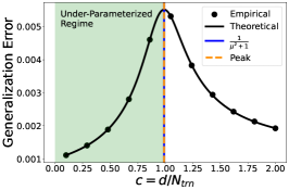
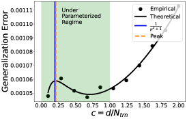
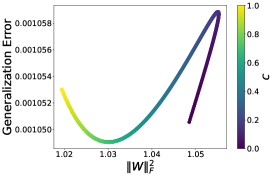
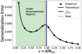
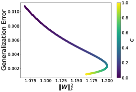
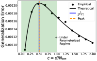
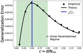
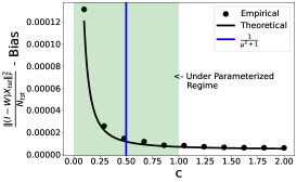
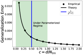
We numerically verify the predictions from Theorems 1, 2, 3. Figure 2 shows that the theoretically predicted risk matches the numerical risk. Moreover, the curve has a single peak for $c<1$. Thus, verifying that double descent occurs in the under-parameterized regime. Finally, Figure 2 shows that the location of the peak is near the conjectured location of $\frac{1}{\mu^{2}+1}$. This conjecture is further tested for a larger range of $\mu$ values in Appendix B. One similarity with prior work is that the peak in the generalization error or risk is corresponds to a peak in the norm of the estimator $W_{opt}$ as seen in Figure 3 (i.e., the curve passes through the top right corner). The figure further shows, as conjectured in [76], that the double descent for the generalization error disappears when plotted as a function of $\|W_{opt}\|_{F}^{2}$ and, in some cases, recovers an approximation of the standard U shaped error curve.

Figure 4: Figure showing that the shape of the risk curve in the data scaling regime depends on $d$ [(L) $d=1000$, (R) $d=2000$]. Here $\mu=\sqrt{2},\sigma_{trn}=\sqrt{N_{tst}},\sigma_{trn}=\sqrt{N_{tst}},N_{tst}=1000$. Each empirical point is an average of at least 200 trials. More details can be found in Appendix D.

Risk curve shape depends on $d$.

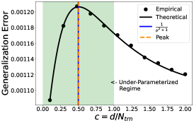
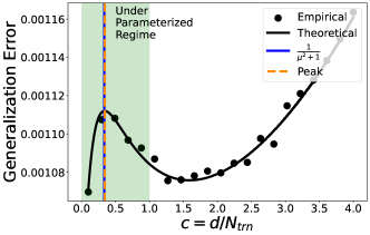
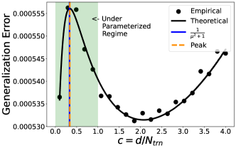
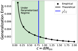
Another interesting aspect of Theorem 2 is that it requires that $d$ is large enough. Hence the shape of the risk curve depends on $d$. Most results for the risk are in the asymptotic regime. While Theorems 1, 2, and 3 are also in the asymptotic regime, we see that the results are accurate even for (relatively) small values of $d,N_{trn}$. Figure 4 shows that the shape of the risk curve depends on the value of $d$. Both curves still have a peak at the same location.

Parameter Scaling.

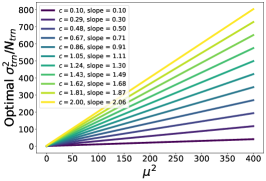
For many prior models, the data scaling and parameter scaling regimes are analogous in that the shape of the risk curve does not depend on which one is scaled. The shape is primarily governed by the aspect ratio $c$ of the data matrix. However, we see significant differences between the parameter scaling and data scaling regimes for our setup. Figure 5 shows risk curves that differ from those in Figure 2. Further, while for small values of $\mu$, double descent occurs in the under-parameterized regime, for larger values of $\mu$, the risk is monotonically decreasing.

Figure 5: Figure showing the risk curves in the parameter scaling regime for different values of $\mu$ [(L) $\mu=0.1$, (C) $\mu=0.2$, (R) $\mu=0.2$]. Here only the $\mu=0.1$ has a local peak. Here $N_{trn}=N_{tst}=1000$ and $\sigma_{trn}=\sigma_{tst}=\sqrt{1000}$. Each empirical point is an average of 100 trials.

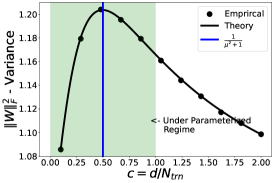
Even more astonishing, as shown in Figure 6, is the fact that for larger values of $\mu$, there is still a peak in the curve for the norm of the estimator $\|W_{opt}\|_{F}^{2}$. However, this does not translate to a peak in the risk curve. Thus, showing that the norm of the estimator increasing cannot solely result in the generalization error increasing. The following theorem provides a local maximum in the $\|W_{opt}\|_{F}^{2}$ versus $c$ curve for $c<1$.

Theorem 4 ($\|W_{opt}\|_{F}$ Peak).

If $\sigma_{tst}=\sqrt{N_{tst}}$, $\sigma_{trn}=\sqrt{N_{trn}}$ and $\mu$ is such that $p(\mu)<0$, then for $N_{trn}$ large enough and $d=cN_{trn}$, we have that $\|W_{opt}\|_{F}$ has a local maximum in the under-parameterized regime. Specifically for $c\in((\mu^{2}+1)^{-1},1)$.

(a)

(b)

(c)

Figure 6: Figure showing generalization error versus $\|W_{opt}\|_{F}^{2}$ for the parameter scaling regime for three different values of $\mu$. More details can be found in Appendix B.

Training Error.

Figure 7: Figure showing the training error, the third derivative of the training error, and the location of the peak of the generalization error for different values of $\mu$ [(L) $\mu=1$, (C) $\mu=2$] for the data scaling regime. (R) shows the location of the local minimum of the third derivative and $\frac{1}{\mu^{2}+1}$.

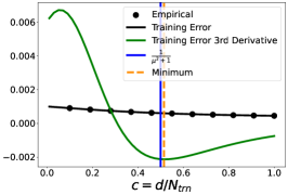
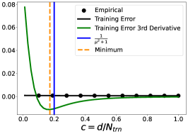
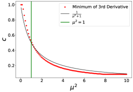
As seen in the prior section, the peak happens in the interior of the under-parameterized regime and not on the border between the under-parameterized and over-parameterized regimes. In many prior works, the peak aligns with the interpolation point (i.e., zero training error). Theorem 5 derives a formula for the training error in the under-parameterized regime. Figure 7 plots the location of the peak, the training error, and the third derivative of the training error. Here the figure shows that the training error curve does not signal the location of the peak in the generalization error curve. However, it shows that for the data scaling regime, the peak roughly corresponds to a local minimum of the third derivative of the training error.

Theorem 5 (Training Error).

Let $\tau$ be as in Theorem 1. The training error for $c<1$ is given by

$$\mathbb{E}_{A_{trn}}[\|X_{trn}-W_{opt}(X_{trn}+A_{trn})\|_{F}^{2}]=\tau^{-2}\left(\sigma_{trn}^{2}\left(1-c\cdot T_{1}\right)+\sigma^{4}_{trn}T_{2}\right)+o(1),$$

where $\displaystyle T_{1}=\frac{\mu^{2}}{2}\left(\frac{1+c+\mu^{2}c}{\sqrt{(1-c+\mu^{2}c)^{2}+4\mu^{2}c^{2}}}-1\right)+\frac{1}{2}+\frac{1+\mu^{2}c-\sqrt{(1-c+\mu^{2}c)^{2}+4c^{2}\mu^{2}}}{2c}$, and $\displaystyle T_{2}=\frac{(\mu^{2}c+c-1-\sqrt{(1-c+\mu^{2}c)^{2}+4c^{2}\mu^{2}})^{2}(\mu^{2}c+c+1-\sqrt{(1-c+\mu^{2}c)^{2}+4c^{2}\mu^{2}})}{2\sqrt{(1-c+\mu^{2}c)^{2}+4c^{2}\mu^{2}}}$.

4 Regularization Trade-off

We analyze the trade-off between the two regularizers and the generalization error.

Figure 8: The first two figures show the $\sigma_{trn}$ versus risk curve for $c=0.5,\mu=1$ and $c=2,\mu=0.1$ with $d=1000$. The second two figures show the risk when training using the optimal $\sigma_{trn}$ for the data scaling and parameter scaling regimes.

Optimal $\sigma_{trn}$.

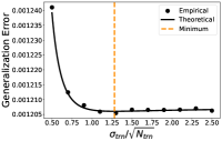
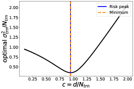
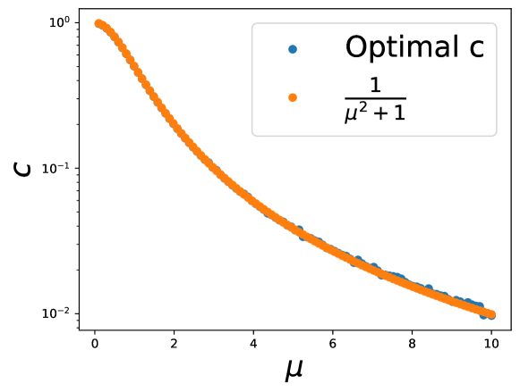
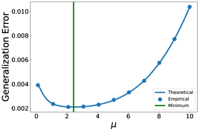
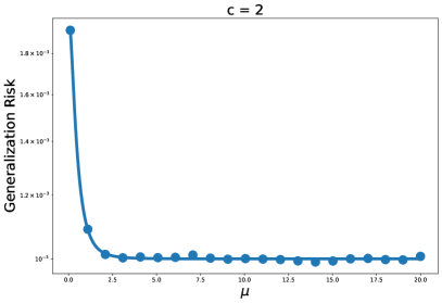
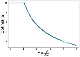
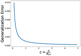
First, we fix $\mu$ and determine the optimal $\sigma_{trn}$. Figure 8 displays the generalization error versus $\sigma_{trn}^{2}$ curve. The figure shows that the error is initially large but then decreases until the optimal generalization error. The generalization error when using the optimal $\sigma_{trn}$ is also shown in Figure 8. Here, unlike [24], picking the optimal value of $\sigma_{trn}$ does not mitigate double descent.

Proposition 1 (Optimal $\sigma_{trn}$).

The optimal value of $\sigma_{trn}^{2}$ for $c<1$ is given by

$$\sigma_{trn}^{2}=\frac{\sigma_{tst}^{2}d[2c(\mu^{2}+1)^{2}-2T(c\mu^{2}+c+1)+2(c\mu^{2}-2c+1)]+N_{tst}(\mu^{2}c^{2}+c^{2}+1-T)}{N_{tst}(c^{3}(\mu^{2}+1)^{2}-T(\mu^{2}c^{2}+c^{2}-1)-2c^{2}-1)}.$$

Figure 9: The first figure plots the optimal $\sigma_{trn}^{2}/N_{trn}$ versus $\mu$ curve. The middle figure plots the optimal $\sigma_{trn}^{2}/N_{trn}$ versus $c$ in the data scaling regime for $\mu=0.5$, and the last figure plots the optimal $\sigma_{trn}^{2}/N_{trn}$ versus $c$ in the parameter scaling regime for $\mu=0.1$.

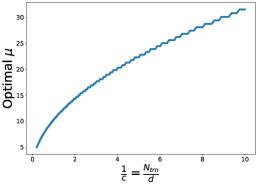
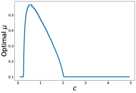
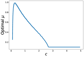
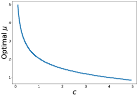
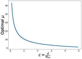
Additionally, it is interesting to determine how the optimal value of $\sigma_{trn}$ depends on both $\mu$ and $c$. Figure 9 shows that for small values of $\mu$ (0.1,0.5), as $c$ changes, there exists an (inverted) double descent curve for the optimal value of $\sigma_{trn}$. However, unlike [34], for the data scaling regime, the minimum of this double descent curve does not match the location for the peak of the generalization error. Further, as the amount of ridge regularization increases, the optimal amount of noise regularization decreases proportionally; optimal $\sigma_{trn}^{2}\approx d\mu^{2}$. Thus, for higher values of ridge regularization, it is preferable to have higher-quality data.

Interaction Between the Regularizers.

Figure 10: Trade-off between the regularizers. The left column is the optimal $\sigma_{trn}$, the central column is the optimal $\mu$, and the right column is the generalization error for these parameter restrictions.

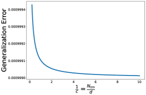
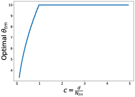
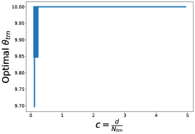
The optimal values of $\mu$ and $\sigma_{trn}$ are jointly computed using grid search for $\mu\in(0,100]$ and $\sigma_{trn}/\sqrt{N_{trn}}\in(0,10]$. Figure 10 shows the results. Specifically, $\sigma_{trn}$ is at the highest possible value (so best quality data), and then the model regularizes purely using the ridge regularizer. This results in a monotonically decreasing generalization error curve. Thus, in the data scaling model, there is an implicit bias that favors one regularizer over the other. Specifically, the model’s implicit bias is to use higher quality data while using ridge regularization to regularize the model appropriately. It is surprising that the two regularizers are not balanced.

5 Conclusion

This paper presented a simple model with double descent in the under-parameterized regime for the data scaling and parameter scaling regimes. We also see that the three prevalent theories for the location of the peak, i.e., at the boundary between the under and over-parameterized regimes, at the interpolation point, and at the point where the norm of estimator peaks, do not explain the peak for this model. Specifically, we show that the peak in the data scaling regime is near $c=1/(\mu^{2}+1)$, where $\mu$ is the ridge regularization coefficient. In the parameter-scaling regime, we show that for large values of $\mu$, we still have a peak in the curve for $\|W_{opt}\|_{F}$ versus the number of parameters. But this no longer corresponds to a peak in the generalization error curve. Hence to provide a general theory, further investigations into the cause and the locations of peaks in the generalization error curve is required.

Appendix A Proofs

A.1 Linear Regression

We begin by noting,

$$\beta^{T}=(\beta_{opt}^{T}X+\xi_{trn})X_{trn}^{\dagger}.$$

Thus, we have,

$$\|\beta\|^{2} =\operatorname{Tr}(\beta^{T}\beta)$$

$$=\operatorname{Tr}(\beta_{opt}^{T}X_{trn}X_{trn}^{\dagger}(X_{trn}^{\dagger})^{T}X_{trn}\beta_{opt})+\operatorname{Tr}(\xi_{trn}X_{trn}^{\dagger}(X_{trn}^{\dagger})^{T}\xi_{trn}^{T})+2\operatorname{Tr}(\beta_{opt}^{T}X_{trn}X_{trn}^{\dagger}X_{trn}^{\dagger})^{T}\xi_{trn}^{T}.$$

Taking the expectation, with respect to $\xi_{trn}$, we see that the last term vanishes.

Letting $X_{trn}=U_{X}\Sigma_{X}V_{X}^{T}$. We see that using the rotational invariance of $X$, $U_{X},V_{X}$ are independent and uniformly random. Thus, $s:=\beta_{opt}^{T}U_{X}$ is a uniformly random unit vector.

Thus, we see,

$$\mathbb{E}_{X_{trn},\xi_{trn}}\left[\operatorname{Tr}(\beta_{opt}^{T}X_{trn}X_{trn}^{\dagger}(X_{trn}^{\dagger})^{T}X_{trn}\beta_{opt})\right]=\sum_{i=1}^{\min(d,N_{trn})}\mathbb{E}[s_{i}^{2}]=\min\left(1,\frac{1}{c}\right)$$

Similarly, we see,

$$\mathbb{E}_{X_{trn},\xi_{trn}}\left[\xi_{trn}X_{trn}^{\dagger}(X_{trn}^{\dagger})^{T}\xi_{trn}^{T}\right]=\sum_{i=1}^{\min(d,N_{trn})}\mathbb{E}\left[\frac{1}{\sigma_{i}(X_{trn})^{2}}\right]$$

Multiplying and dividing by $d$, normalizes the singular values squared of $X_{trn}$ so that the limiting distribution is the Marchenko Pastur distribution with shape $c$. Thus, we can estimate using Lemma 5 from [34] to get,

$$\begin{cases}\frac{c}{1-c}+o(1)&c<1\\ \frac{1}{c-1}+o(1)&c>1\end{cases}.$$

Finally, the cross-term has an expectation equal to zero. Thus,

$$\mathbb{E}_{X_{trn},\xi_{trn}}[\|\beta_{opt}\|^{2}]=\begin{cases}1+\frac{c}{1-c}&c<1\\ \frac{1}{c}+\frac{1}{c-1}&c>1\end{cases}$$

Then we have,

$$\beta^{T}\beta_{opt}=\beta_{opt}^{T}X_{trn}X_{trn}^{\dagger}\beta_{opt}+\xi_{trn}X_{trn}^{\dagger}\beta_{opt}$$

The second term has an expectation equal to zero, and the first term is similar to before and has an expectation equal to $\displaystyle\min\left(1,\frac{1}{c}\right)$.

A.2 Proofs for Theorem 1

The proof structure closely follows that of [34].

A.2.1 Step 1: Decompose the error into bias and variance terms.

First, we decompose the error. Since we are not in the supervised learning setup, we do not have standard definitions of bias/variance. However, we will call the following terms the bias/variance of the model. First, we recall the following from [34].

Lemma 1 ([34]).

If $A_{tst}$ has mean 0 entries and $A_{tst}$ is independent of $X_{tst}$ and $W$, then

$$\begin{split}\mathbb{E}_{A_{tst}}[\|X_{tst}-WY_{tst}\|^{2}_{F}]&=\underbrace{\mathbb{E}_{A_{tst}}[\|X_{tst}-WX_{tst}\|^{2}_{F}]}_{Bias}+\underbrace{\mathbb{E}_{A_{tst}}[\|WA_{tst}\|^{2}_{F}]}_{Variance}.\end{split}$$ (4)

A.2.2 Step 2: Formula for $W_{opt}$

Here, we compute the explicit formula for $W_{opt}$ in Problem 1. Let $\hat{A}_{trn}=\left[A_{trn}\quad\mu I\right]$, $\hat{X}_{trn}=\left[X_{trn}\quad 0\right]$ , and $\hat{Y}_{trn}=\hat{X}_{trn}+\hat{A}_{trn}$. Then solving $\operatorname*{arg\,min}_{W}\|X_{trn}-WY_{trn}\|_{F}^{2}+\mu^{2}\|W\|_{F}^{2}$ is equivalent to solving $\operatorname*{arg\,min}_{W}\|\hat{X}_{trn}-W\hat{Y}_{trn}\|_{F}^{2}$. Thus, $W_{opt}=\operatorname*{arg\,min}_{W}\|\hat{X}_{trn}-W\hat{Y}_{trn}\|_{F}^{2}=\hat{X}_{trn}\hat{Y}_{trn}^{\dagger}$. Expanding this out, we get the following formula for $\hat{W}$. Let $\hat{u}$ be the left singular vector and $\hat{v}_{trn}$ be the right singular vectors of $\hat{X}_{trn}$. Note that the left singular does not change after ridge regularization, so $\hat{u}=u$. Let $\hat{h}=\hat{v}_{trn}^{T}\hat{A}_{trn}^{\dagger}$, $\hat{k}=\hat{A}_{trn}^{\dagger}u$, $\hat{s}=(I-\hat{A}_{trn}\hat{A}_{trn}^{\dagger})u$, $\hat{t}=\hat{v}_{trn}(I-\hat{A}_{trn}^{\dagger}\hat{A}_{trn})$, $\hat{\gamma}=1+\sigma_{trn}\hat{v}_{trn}^{T}\hat{A}_{trn}^{{\dagger}}u$, $\hat{\tau}=\sigma_{trn}^{2}\|\hat{t}\|^{2}\|\hat{k}\|^{2}+\hat{\gamma}^{2}$.

Proposition 2.

If $\hat{\gamma}\neq 0$ and $A_{trn}$ has full rank then

$$W_{opt}=\frac{\sigma_{trn}\hat{\gamma}}{\hat{\tau}}u\hat{h}+\frac{\sigma_{trn}^{2}\|\hat{t}\|^{2}}{\hat{\tau}}u\hat{k}^{T}\hat{A}_{trn}^{\dagger}.$$

Proof.

Here we know that $u$ is arbitrary. We have that $\hat{A}_{trn}$ has full rank. Thus, the rank of $\hat{A}_{trn}$ is $d$, and the range of $\hat{A}_{trn}$ is the whole space. Thus, $u$ lives in the range of $\hat{A}_{trn}$. In this case, we want Theorem 3 from [77]. We define

$$\hat{p}=-\frac{\sigma_{trn}^{2}\|\hat{k}\|^{2}}{\hat{\gamma}}\hat{t}^{T}-\sigma_{trn}\hat{k}\text{ and }\hat{q}^{T}=-\frac{\sigma_{trn}\|\hat{t}\|^{2}}{\hat{\gamma}}\hat{k}^{T}\hat{A}_{trn}^{\dagger}-\hat{h}.$$

Then we have,

$$(\hat{A}_{trn}+\sigma_{trn}u\hat{v}_{trn}^{T})^{\dagger}=\hat{A}_{trn}^{\dagger}+\frac{\sigma_{trn}}{\hat{\gamma}}\hat{t}^{T}\hat{k}^{T}\hat{A}_{trn}^{\dagger}-\frac{\hat{\gamma}}{\hat{\tau}}\hat{p}\hat{q}^{T}.$$

Note that, by our assumptions, we have $\hat{t}=\hat{v}_{trn}(I-\hat{A}_{trn}^{\dagger}\hat{A}_{trn})$, and $(I-\hat{A}_{trn}^{\dagger}\hat{A}_{trn})$ is a projection matrix, thus

$$\hat{v}_{trn}^{T}\hat{t}^{T} =\hat{v}_{trn}^{T}(I-\hat{A}_{trn}^{\dagger}\hat{A}_{trn})^{T}\hat{v}_{trn}^{T}$$

$$=\hat{v}_{trn}^{T}(I-\hat{A}_{trn}^{\dagger}\hat{A}_{trn})^{T}(I-\hat{A}_{trn}^{\dagger}\hat{A}_{trn})^{T}\hat{v}_{trn}^{T}.$$

To compute $W_{opt}=\hat{X}_{trn}(\hat{X}_{trn}+\hat{A}_{trn})^{\dagger}=\sigma_{trn}u\hat{v}_{trn}^{T}(\hat{A}_{trn}+\sigma_{trn}u\hat{v}_{trn}^{T})^{\dagger}$, using $\hat{\gamma}-1=\sigma_{trn}\hat{v}_{trn}^{T}\hat{A}_{trn}^{\dagger}u=\sigma_{trn}\hat{h}u$, we multiply this through.

$$\sigma_{trn}u\hat{v}_{trn}^{T}(\hat{A}_{trn}+\sigma_{trn}u\hat{v}_{trn}^{T})^{\dagger} =\sigma_{trn}u\hat{v}_{trn}^{T}(\hat{A}_{trn}^{\dagger}+\frac{\sigma_{trn}}{\hat{\gamma}}\hat{t}^{T}\hat{k}^{T}\hat{A}_{trn}^{\dagger}-\frac{\hat{\gamma}}{\hat{\tau}}\hat{p}\hat{q}^{T})$$

$$=\sigma_{trn}u\hat{h}+\frac{\sigma_{trn}^{2}\|\hat{t}\|^{2}}{\hat{\gamma}}u\hat{k}^{T}\hat{A}_{trn}^{\dagger}$$

$$\ \ \ \ +\frac{\sigma_{trn}\hat{\gamma}}{\hat{\tau}}u\hat{v}_{trn}^{T}\left(\frac{\sigma_{trn}^{2}\|\hat{k}\|^{2}}{\hat{\gamma}}\hat{t}^{T}+\sigma_{trn}\hat{k}\right)\hat{q}^{T}$$

$$=\sigma_{trn}u\hat{h}+\frac{\sigma_{trn}^{2}\|\hat{t}\|^{2}}{\hat{\gamma}}u\hat{k}^{T}\hat{A}_{trn}^{\dagger}+\frac{\sigma_{trn}^{3}\|\hat{k}\|^{2}\|\hat{t}\|^{2}}{\hat{\tau}}u\hat{q}^{T}$$

$$\ \ \ \ +\frac{\sigma_{trn}\hat{\gamma}(\hat{\gamma}-1)}{\hat{\tau}}u\hat{q}^{T}.$$

Then we have,

$$\frac{\sigma_{trn}^{3}\|\hat{k}\|^{2}\|\hat{t}\|^{2}}{\hat{\tau}}u\hat{q}^{T} =\frac{\sigma_{trn}^{3}\|\hat{k}\|^{2}\|\hat{t}\|^{2}}{\hat{\tau}}u\left(-\frac{\sigma_{trn}\|\hat{t}\|^{2}}{\hat{\gamma}}\hat{k}^{T}\hat{A}_{trn}^{\dagger}-\hat{h}\right)$$

$$=-\frac{\sigma_{trn}^{4}\|\hat{k}\|^{2}\|\hat{t}\|^{4}}{\hat{\tau}\hat{\gamma}}u\hat{k}^{T}\hat{A}_{trn}^{\dagger}-\frac{\sigma_{trn}^{3}\|\hat{k}\|^{2}\|\hat{t}\|^{2}}{\hat{\tau}}u\hat{h}$$

and

$$\frac{\sigma_{trn}\hat{\gamma}(\hat{\gamma}-1)}{\hat{\tau}}u\hat{q}^{T} =\frac{\sigma_{trn}\hat{\gamma}(\hat{\gamma}-1)}{\hat{\tau}}u\left(-\frac{\sigma_{trn}\|\hat{t}\|^{2}}{\hat{\gamma}}\hat{k}^{T}\hat{A}_{trn}^{\dagger}-\hat{h}\right)$$

$$=-\frac{\sigma_{trn}^{2}\|\hat{t}\|^{2}(\hat{\gamma}-1)}{\hat{\tau}}u\hat{k}^{T}\hat{A}_{trn}^{\dagger}-\frac{\sigma_{trn}\hat{\gamma}(\hat{\gamma}-1)}{\hat{\tau}}u\hat{h}.$$

Substituting back in and collecting like terms, we get,

$$\sigma_{trn}u\hat{v}_{trn}^{T}(\hat{A}_{trn}+\sigma_{trn}u\hat{v}_{trn}^{T})^{\dagger} =\sigma_{trn}\left(1-\frac{\sigma_{trn}^{2}\|\hat{k}\|^{2}\|\hat{t}\|^{2}}{\hat{\tau}}-\frac{\hat{\gamma}(\hat{\gamma}-1)}{\hat{\tau}}\right)u\hat{h}+$$

$$\sigma_{trn}^{2}\left(\frac{\|\hat{t}\|^{2}}{\hat{\gamma}}-\frac{\sigma_{trn}^{2}\|\hat{k}\|^{2}\|\hat{t}\|^{4}}{\hat{\tau}\hat{\gamma}}-\frac{\|\hat{t}\|^{2}(\hat{\gamma}-1)}{\hat{\tau}}\right)u\hat{k}^{T}\hat{A}_{trn}^{\dagger}.$$

We can then simplify the constants as follows.

$$1-\frac{\sigma_{trn}^{2}\|\hat{k}\|^{2}\|\hat{t}\|^{2}}{\hat{\tau}}-\frac{\hat{\gamma}(\hat{\gamma}-1)}{\hat{\tau}}=\frac{\hat{\tau}-\sigma_{trn}^{2}\|\hat{k}\|^{2}\|\hat{t}\|^{2}-\gamma^{2}+\gamma}{\hat{\tau}}=\frac{\hat{\gamma}}{\hat{\tau}}$$

and

$$\frac{\|\hat{t}\|^{2}}{\hat{\gamma}}-\frac{\sigma_{trn}^{2}\|\hat{k}\|^{2}\|\hat{t}\|^{4}}{\hat{\tau}\hat{\gamma}}-\frac{\|\hat{t}\|^{2}(\hat{\gamma}-1)}{\hat{\tau}}=\frac{\|\hat{t}\|^{2}\left(\hat{\tau}-\sigma_{trn}^{2}\|\hat{k}\|^{2}\|\hat{t}\|^{2}-\hat{\gamma}^{2}+\hat{\gamma}\right)}{\hat{\tau}\hat{\gamma}}=\frac{\|\hat{t}\|^{2}}{\hat{\tau}}.$$

This gives us the result. ∎

A.2.3 Step 3: Decompose the terms into a sum of various trace terms.

For the bias and variance terms, we have the following two Lemmas.

Lemma 2.

If $W_{opt}$ is the solution to Equation 1, then

$$X_{tst}-W_{opt}X_{tst}=\frac{\hat{\gamma}}{\hat{\tau}}X_{tst}.$$

Proof.

To see this, note that we have $N_{trn}+M>M$.

$$X_{tst}-W_{opt}X_{tst} =X_{tst}-\frac{\sigma_{trn}\hat{\gamma}}{\hat{\tau}}u\hat{h}uv_{tst}^{T}-\frac{\sigma_{trn}^{2}\|\hat{t}\|^{2}}{\hat{\tau}}u\hat{k}^{T}\hat{A}_{trn}^{\dagger}uv_{tst}^{T}$$

$$=X_{tst}-\frac{\hat{\sigma}_{trn}\hat{\gamma}}{\hat{\tau}}u\hat{v}_{trn}^{T}\hat{A}_{trn}^{\dagger}uv_{tst}^{T}-\frac{\sigma_{trn}^{2}\|\hat{t}\|^{2}}{\hat{\tau}}u\hat{k}^{T}\hat{A}_{trn}^{\dagger}uv_{tst}^{T}.$$

Note that $\hat{\gamma}=1+\sigma_{trn}\hat{v}_{trn}^{T}\hat{A}_{trn}^{\dagger}u$. Thus, we have that $\sigma_{trn}\hat{v}_{trn}^{T}\hat{A}_{trn}^{\dagger}u=\hat{\gamma}-1$. Substituting this into the second term, we get,

$$X_{tst}-W_{opt}X_{tst}=X_{tst}-\frac{\hat{\gamma}(\hat{\gamma}-1)}{\hat{\tau}}uv_{tst}^{T}-\frac{\sigma_{trn}^{2}\|\hat{t}\|^{2}}{\hat{\tau}}u\hat{k}^{T}\hat{A}_{trn}^{\dagger}uv_{tst}^{T}.$$

For the third term, since $\hat{k}=\hat{A}_{trn}^{\dagger}u$, $\hat{k}^{T}\hat{A}_{trn}^{\dagger}u=\hat{k}^{T}\hat{k}=\|\hat{k}\|^{2}$. Substituting this into the expression, we get that

$$X_{tst}-W_{opt}X_{tst}=X_{tst}-\frac{\hat{\gamma}(\hat{\gamma}-1)}{\hat{\tau}}uv_{tst}^{T}-\frac{\sigma_{trn}^{2}\|\hat{t}\|^{2}\|\hat{k}\|^{2}}{\hat{\tau}}uv_{tst}^{T}.$$

Since $X_{tst}=uv_{tst}^{T}$, we get,

$$X_{tst}-W_{opt}X_{tst}=X_{tst}\left(1-\frac{\hat{\gamma}(\hat{\gamma}-1)}{\hat{\tau}}-\frac{\sigma_{trn}^{2}\|\hat{t}\|^{2}\|\hat{k}\|^{2}}{\hat{\tau}}\right).$$

Simplify the constants using $\hat{\tau}=\sigma_{trn}^{2}\|\hat{t}\|^{2}\|\hat{k}\|^{2}+\hat{\gamma}^{2}$, we get,

$$\frac{\hat{\tau}+\hat{\gamma}-\hat{\gamma}^{2}-\sigma_{trn}^{2}\|\hat{t}\|^{2}\|\hat{k}\|^{2}}{\hat{\tau}}=\frac{\hat{\gamma}}{\hat{\tau}}.$$

∎

Lemma 3 ([34]).

If the entries of $A_{tst}$ are independent with mean 0, and variance $1/d$, then we have that $\mathbb{E}_{A_{tst}}[\|W_{opt}A_{tst}\|^{2}]=\frac{N_{tst}}{d}\|W_{opt}\|^{2}$.

Lemma 4.

If $\hat{\gamma}\neq 0$ and $A_{trn}$ has full rank, then we have that

$$\|W_{opt}\|_{F}^{2}=\frac{\sigma_{trn}^{2}\hat{\gamma}^{2}}{\tau^{2}}\operatorname{Tr}(\hat{h}^{T}\hat{h})+2\frac{\sigma_{trn}^{3}\|\hat{t}\|^{2}\hat{\gamma}}{\hat{\tau}^{2}}\operatorname{Tr}(\hat{h}^{T}\hat{k}^{T}\hat{A}_{trn}^{\dagger})+\frac{\sigma_{trn}^{4}\|\hat{t}\|^{4}}{\hat{\tau}^{2}}\underbrace{\operatorname{Tr}((\hat{A}_{trn}^{\dagger})^{T}\hat{k}\hat{k}^{T}\hat{A}_{trn}^{\dagger})}_{\rho}.$$

Proof.

We have

$$\|W_{opt}\|_{F}^{2} =\operatorname{Tr}(W_{opt}^{T}W_{opt})$$

$$=\operatorname{Tr}\left(\left(\frac{\sigma_{trn}\hat{\gamma}}{\hat{\tau}}u\hat{h}+\frac{\sigma_{trn}^{2}\|\hat{t}\|^{2}}{\hat{\tau}}u\hat{k}^{T}\hat{A}_{trn}^{\dagger}\right)^{T}\left(\frac{\sigma_{trn}\hat{\gamma}}{\hat{\tau}}u\hat{h}+\frac{\sigma_{trn}^{2}\|\hat{t}\|^{2}}{\hat{\tau}}u\hat{k}^{T}\hat{A}_{trn}^{\dagger}\right)\right)$$

$$=\frac{\sigma_{trn}^{2}\hat{\gamma}^{2}}{\hat{\tau}^{2}}\operatorname{Tr}(\hat{h}^{T}u^{T}u\hat{h})+2\frac{\sigma_{trn}^{3}\|\hat{t}\|^{2}\hat{\gamma}}{\hat{\tau}^{2}}\operatorname{Tr}(\hat{h}^{T}u^{T}u\hat{k}^{T}\hat{A}_{trn}^{\dagger})$$

$$\ \ \ \ +\frac{\sigma_{trn}^{4}\|\hat{t}\|^{4}}{\hat{\tau}^{2}}\operatorname{Tr}((\hat{A}_{trn}^{\dagger})^{T}\hat{k}u^{T}u\hat{k}^{T}\hat{A}_{trn}^{\dagger})$$

$$=\frac{\sigma_{trn}^{2}\hat{\gamma}^{2}}{\hat{\tau}^{2}}\operatorname{Tr}(\hat{h}^{T}\hat{h})+2\frac{\sigma_{trn}^{3}\|\hat{t}\|^{2}\hat{\gamma}}{\hat{\tau}^{2}}\operatorname{Tr}(\hat{h}^{T}\hat{k}^{T}\hat{A}_{trn}^{\dagger})+\frac{\sigma_{trn}^{4}\|\hat{t}\|^{4}}{\hat{\tau}^{2}}\operatorname{Tr}((\hat{A}_{trn}^{\dagger})^{T}\hat{k}\hat{k}^{T}\hat{A}_{trn}^{\dagger}).$$

Where the last inequality is true due to the fact that $\|u\|^{2}=1$. ∎

A.2.4 Step 4: Estimate With Random Matrix Theory

Lemma 5.

Let $A$ be a $p\times q$ matrix and let $\hat{A}=[A\quad\mu I]\in\mathbb{R}^{p\times q+p}$. Suppose $A=U\Sigma V^{T}$ be the singular value decomposition of $A$. If $\hat{A}=\hat{U}\hat{\Sigma}\hat{V}^{T}$ is the singular value decomposition of $\hat{A}$, then $\hat{U}=U$ and if $p<q$

$$\hat{\Sigma}=\begin{bmatrix}\sqrt{\sigma_{1}(A)^{2}+\mu^{2}}&0&\cdots&0\\ 0&\sqrt{\sigma_{2}(A)^{2}+\mu^{2}}&&0\\ \vdots&&\ddots&\vdots\\ 0&0&\cdots&\sqrt{\sigma_{p}(A)^{2}+\mu^{2}}\end{bmatrix}\in\mathbb{R}^{p\times p},$$

and

$$\hat{V}=\begin{bmatrix}V_{1:p}\Sigma\hat{\Sigma}^{-1}\\ \mu U\hat{\Sigma}^{-1}\end{bmatrix}\in\mathbb{R}^{q+p\times p}.$$

Here $V_{1:p}$ are the first $p$ columns of $V$.

Proof.

Since $p<q$, we have that $U\in\mathbb{R}^{p\times p}$, $\Sigma\in\mathbb{R}^{p\times p}$ are invertible. Here also consider the form of the SVD in which $V^{T}\in\mathbb{R}^{p\times q}$.

We start by nothing that $\hat{U}\hat{\Sigma}^{2}\hat{U}^{T}=\hat{A}\hat{A}^{T}=AA^{T}+\mu^{2}I=U(\Sigma^{2}+\mu^{2}I_{p})U^{T}$. Thus, we immediately see that $\sigma_{i}(\hat{A})^{2}=\sigma_{i}(A)^{2}+\mu^{2}$ and that $\hat{U}=U$.

Finally, we see,

$$\hat{V}^{T}=\hat{\Sigma}^{-1}U^{T}\hat{A}=\begin{bmatrix}\hat{\Sigma}^{-1}\Sigma V_{1:p}^{T}&\mu\hat{\Sigma}^{-1}U^{T}\end{bmatrix}$$

∎

Lemma 6.

Let $A$ be a $p\times q$ matrix and let $\hat{A}=[A\quad\mu I]\in\mathbb{R}^{p\times q+p}$. Suppose $A=U\Sigma V^{T}$ be the singular value decomposition of $A$. If $\hat{A}=\hat{U}\hat{\Sigma}\hat{V}^{T}$ is the singular value decomposition of $\hat{A}$, then $\hat{U}=U$ and if $p>q$

$$\hat{\Sigma}=\begin{bmatrix}\sqrt{\sigma_{1}(A)^{2}+\mu^{2}}&0&\cdots&0&&\cdots&0\\ 0&\sqrt{\sigma_{2}(A)^{2}+\mu^{2}}&&0&&&\\ \vdots&&\ddots&\vdots&&&\vdots\\ 0&0&\cdots&\sqrt{\sigma_{q}(A)^{2}+\mu^{2}}&&&0\\ &&&&\mu&&\\ \vdots&&&&&\ddots&0\\ 0&0&\cdots&0&\cdots&0&\mu\end{bmatrix}\in\mathbb{R}^{p\times p}.$$

Here we will denote the upper left $q\times q$ block by $C$. Further,

$$\hat{V}=\begin{bmatrix}V\Sigma_{1:q,1:q}^{T}C^{-1}&0\\ \mu U_{1:q}C^{-1}&U_{q+1:p}\end{bmatrix}\in\mathbb{R}^{q+p\times p}.$$

Proof.

Since $p>q$, we have that $U\in\mathbb{R}^{p\times p}$ and we have that $\Sigma\in\mathbb{R}^{p\times q}$. Here $V^{T}\in\mathbb{R}^{q\times q}$ is invertible.

We start with nothing,

$$\hat{U}\hat{\Sigma}^{2}\hat{U}^{T}=\hat{A}\hat{A}^{T}=AA^{T}+\mu^{2}I=U\left(\begin{bmatrix}\Sigma_{1:q,1:q}^{2}&0\\ 0&0_{q-p}\end{bmatrix}+\mu^{2}I_{q}\right)U^{T}.$$

Thus, we immediately see that for $i=1,\ldots,p$ $\sigma_{i}(\hat{A})^{2}=\sigma_{i}(A)^{2}+\mu^{2}$ and for $i=p+1,\ldots,q$, we have that $\sigma_{i}(\hat{A})^{2}=\mu^{2}$ and that $\hat{U}=U$.

Then, we see,

$$\hat{V}^{T}=\hat{\Sigma}^{-1}U^{T}\hat{A}=\begin{bmatrix}\hat{\Sigma}^{-1}\Sigma V^{T}&\mu\hat{\Sigma}^{-1}U^{T}\end{bmatrix}.$$

Note that $\Sigma$ has $0$ for the last $p-q$ entries. Thus,

$$\hat{\Sigma}^{-1}\Sigma V=\begin{bmatrix}C^{-1}\Sigma_{1:q,1:q}V\\ 0_{q-p,q}\end{bmatrix}.$$

Similarly, due to the structure of $\hat{\Sigma}$, we see,

$$\mu\hat{\Sigma}^{-1}U^{T}=[\mu C^{-1}U_{1:q}^{T}\quad\mu\frac{1}{\mu}U_{q+1:p}^{T}].$$

∎

Lemma 7.

Suppose $A$ is an $p$ by $q$ matrix such that $p<q$, the entries of $A$ are independent and have mean 0, variance $1/p$, and bounded fourth moment. Let $c=p/q$. Let $\hat{A}=[A\quad\mu I]\in\mathbb{R}^{p\times q+p}$. Let $W_{p}=\hat{A}\hat{A}^{T}$ and let $W_{q}=\hat{A}^{T}\hat{A}$. Suppose $\lambda_{p}$ is a random non-zero eigenvalue from the largest $p$ eigenvalues of $W_{p}$, and $\lambda_{q}$ is a random non-zero eigenvalue of $W_{q}$. Then

1. $\mathbb{E}\left[\frac{1}{\lambda_{p}}\right]=\mathbb{E}\left[\frac{1}{\lambda_{q}}\right]=\frac{\sqrt{(1+\mu^{2}c-c)^{2}+4\mu^{2}c^{2}}-1-\mu^{2}c+c}{2\mu^{2}c}+o(1)$.

2. $\mathbb{E}\left[\frac{1}{\lambda_{p}^{2}}\right]=\mathbb{E}\left[\frac{1}{\lambda_{q}^{2}}\right]=\frac{\mu^{2}c^{2}+c^{2}+\mu^{2}c-2c+1}{2\mu^{4}c\sqrt{4\mu^{2}c^{2}+(1-c+\mu^{2}c)^{2}}}+\frac{1}{2\mu^{4}}\left(1-\frac{1}{c}\right)+o(1)$.

Proof.

First, we note that the non-zero eigenvalues of $W_{p}$ and $W_{q}$ are the same. Hence we focus on $W_{p}$. $W_{p}$ is nearly a Wishart matrix but is not normalized by the correct value. However, $cW_{p}$ does have the correct normalization.

Due to the assumptions on $A$, we have that the eigenvalues of $cAA^{T}$ converge to the Marchenko-Pastur. Hence since the eigenvalues of $cW_{p}$ are

$$(c\lambda_{p})_{i}=c\sigma_{i}(A)^{2}+c\mu^{2},$$

we can estimate them by estimating $c\sigma_{i}(A)^{2}$ with the Marchenko-Pastur [78, 79, 80, 81, 82]. In particular, we want the expectation of the inverse. We need to use the Stieljes transform. We know that if $m_{c}(z)$ is the Stieljes transform for the Marchenko-Pastur with shape parameter $c$, then if $\lambda$ is sampled from the Marchenko-Pastur distribution, then

$$m_{c}(z)=\mathbb{E}_{\lambda}\left[\frac{1}{\lambda-z}\right].$$

Thus, we have that the expected inverse of the eigenvalue can be approximated $m(-c\mu^{2})$. We know that the Steiljes transform:

$$m_{c}(z)=-\frac{1-z-c-\sqrt{(1-z-c)^{2}-4cz}}{-2zc}.$$

Thus, we have,

$$\mathbb{E}\left[\frac{1}{c\lambda_{p}}\right]=m(-c\mu^{2})=\frac{\sqrt{(1+\mu^{2}c-c)^{2}+4\mu^{2}c^{2}}-1-\mu^{2}c+c}{2\mu^{2}c^{2}}.$$

Canceling $1/c$ from both sides, we get,

$$\mathbb{E}\left[\frac{1}{\lambda_{p}}\right]=\frac{\sqrt{(1+\mu^{2}c-c)^{2}+4\mu^{2}c^{2}}-1-\mu^{2}c+c}{2\mu^{2}c}.$$

Then for the estimate of $\mathbb{E}\left[1/\lambda_{p}^{2}\right]$, we need to compute the derivative of the $m_{c}(z)$ and evaluate it at $-c\mu^{2}$. Hence, we see,

$$m_{c}^{\prime}(z)=\frac{(c-z+\sqrt{-4cz+(1-c-z)^{2}}-1)(c+z+\sqrt{-4cz+(1-c-z)^{2}}-1)}{4cz^{2}\sqrt{-4cz+(1-c-z)^{2}}}.$$

Thus,

$$\mathbb{E}\left[\frac{1}{c^{2}\lambda_{p}^{2}}\right] =m_{c}^{\prime}(-c\mu^{2})$$

$$=\frac{(c+\mu^{2}c+\sqrt{4\mu^{2}c^{2}+(1-c+\mu^{2}c)^{2}}-1)(c-\mu^{2}c+\sqrt{4\mu^{2}c^{2}+(1-c+\mu^{2}c)^{2}}-1)}{4\mu^{4}c^{3}\sqrt{4\mu^{2}c^{2}+(1-c+\mu^{2}c)^{2}}}.$$

Canceling the $1/c^{2}$ from both sides, we get,

$$\mathbb{E}\left[\frac{1}{\lambda_{p}^{2}}\right]=\frac{(c+\mu^{2}c+\sqrt{4\mu^{2}c^{2}+(1-c+\mu^{2}c)^{2}}-1)(c-\mu^{2}c+\sqrt{4\mu^{2}c^{2}+(1-c+\mu^{2}c)^{2}}-1)}{4\mu^{4}c\sqrt{4\mu^{2}c^{2}+(1-c+\mu^{2}c)^{2}}}.$$

Multiplying out and simplifying

$$\mathbb{E}\left[\frac{1}{\lambda_{p}^{2}}\right]=\frac{\mu^{2}c^{2}+c^{2}+\mu^{2}c-2c+1}{2\mu^{4}c\sqrt{4\mu^{2}c^{2}+(1-c+\mu^{2}c)^{2}}}+\frac{1}{2\mu^{4}}\left(1-\frac{1}{c}\right).$$

∎

Lemma 8.

Suppose $A$ is an $p$ by $q$ matrix such that $p>q$, the entries of $A$ are independent and have mean 0, variance $1/p$, and bounded fourth moment. Let $c=p/q$. Let $\hat{A}=[A\quad\mu I]\in\mathbb{R}^{p\times q+p}$. Let $W_{p}=\hat{A}\hat{A}^{T}$ and let $W_{q}=\hat{A}^{T}\hat{A}$. Suppose $\lambda_{p}$ is a random non-zero eigenvalue of $W_{p}$, and $\lambda_{q}$ is a random eigenvalue from the largest $q$ eigenvalues of $W_{q}$. Then

1. $\mathbb{E}\left[\frac{1}{\lambda_{q}}\right]=\mathbb{E}\left[\frac{1}{\lambda_{p}}\right]=\frac{\sqrt{4\mu^{2}c+(1-c+\mu^{2}c)^{2}}-c-\mu^{2}c+1}{2\mu^{2}}+o(1)$.

2. $\mathbb{E}\left[\frac{1}{\lambda_{q}^{2}}\right]=\mathbb{E}\left[\frac{1}{\lambda_{p}^{2}}\right]=\frac{1-2c+c^{2}+\mu^{2}c+\mu^{2}c^{2}}{2\mu^{4}\sqrt{4\mu^{2}c+(-1+c+\mu^{2}c)^{2}}}+(1-c)\frac{1}{2\mu^{4}}+o(1)$.

Proof.

First, we note that the non-zero eigenvalues of $W_{p}$ and $W_{q}$ are the same. Hence we focus on $W_{p}$. Due to the assumptions on $A$, we have that the eigenvalues of $A^{T}A$ converge to the Marchenko-Pastur with shape $c^{-1}$. Hence if $\lambda_{p}$ is one of the first $q$ eigenvalues of $W_{p}$, we see,

$$\mathbb{E}\left[\frac{1}{\lambda_{p}}\right]=m_{c^{-1}}(\mu^{2})=\frac{\sqrt{(1+\mu^{2}-1/c)^{2}+4\mu^{2}/c}-1-\mu^{2}+1/c}{2\mu^{2}/c}.$$

Then for the estimate of $\mathbb{E}\left[1/\lambda_{p}^{2}\right]$, we need to compute the derivative of the $m_{c^{-1}}(z)$ and evaluate it at $-\mu^{2}$. Hence, we see,

$$\mathbb{E}\left[\frac{1}{\lambda_{p}^{2}}\right] =\frac{(1/c+\mu^{2}+\sqrt{4\mu^{2}/c+(1-1/c+\mu^{2})^{2}}-1)(1/c-\mu^{2}+\sqrt{4\mu^{2}/c+(1-1/c+\mu^{2})^{2}}-1)}{4\mu^{4}/c\sqrt{4\mu^{2}/c+(1-1/c+\mu^{2})^{2}}}$$

$$=\frac{(1+\mu^{2}c+c\sqrt{4\mu^{2}/c+(1-1/c+\mu^{2})^{2}}-c)(1-\mu^{2}c+c\sqrt{4\mu^{2}/c+(1-1/c+\mu^{2})^{2}}-c)}{4\mu^{4}c\sqrt{4\mu^{2}/c+(1-1/c+\mu^{2})^{2}}}$$

$$=\frac{(1+\mu^{2}c+\sqrt{4\mu^{2}c+(-1+c+\mu^{2}c)^{2}}-c)(1-\mu^{2}c+\sqrt{4\mu^{2}c+(-1+c+\mu^{2}c)^{2}}-c)}{4\mu^{4}\sqrt{4\mu^{2}c+(-1+c+\mu^{2}c)^{2}}}$$

This can be further simplified to

$$\frac{1-2c+c^{2}+\mu^{2}c+\mu^{2}c^{2}}{2\mu^{4}\sqrt{4\mu^{2}c+(-1+c+\mu^{2}c)^{2}}}+(1-c)\frac{1}{2\mu^{4}}+o(1)$$

∎

We will also need to estimate some other terms.

Lemma 9.

Suppose $A$ is an $p$ by $q$ matrix such that the entries of $A$ are independent and have mean 0, variance $1/p$, and bounded fourth moment. Let $\hat{A}=[A\quad\mu I]\in\mathbb{R}^{p\times q+p}$. Let $W_{p}=\hat{A}\hat{A}^{T}$ and let $W_{q}=\hat{A}^{T}\hat{A}$. Suppose $\lambda_{p},\lambda_{q}$ are random non-zero eigenvalues of $W_{p},W_{q}$ from the largest $\min(p,q)$ eigenvalues of $W_{p},W_{q}$. Then

1. If $p>q$, $\mathbb{E}\left[\frac{\lambda_{p}}{\lambda_{p}+\mu^{2}}\right]=c\left(\frac{1}{2}+\frac{1+\mu^{2}c-\sqrt{(-1+c+\mu^{2}c)^{2}+4\mu^{2}c}}{2c}\right)+o(1)$.

2. If $p<q$, $\mathbb{E}\left[\frac{\lambda_{q}}{\lambda_{q}+\mu^{2}}\right]=\frac{1}{2}+\frac{1+\mu^{2}c-\sqrt{(1-c+\mu^{2}c)^{2}+4c^{2}\mu^{2}}}{2c}+o(1)$.

3. If $p>q$, $\mathbb{E}\left[\frac{\lambda_{p}}{(\lambda_{p}+\mu^{2})^{2}}\right]=c\left(\frac{1+c+\mu^{2}c}{2\sqrt{(-1+c+\mu^{2}c)^{2}+4\mu^{2}c}}-\frac{1}{2}\right)+o(1)$.

4. If $p<q$, $\mathbb{E}\left[\frac{\lambda_{q}}{(\lambda_{q}+\mu^{2})^{2}}\right]=\frac{1+c+\mu^{2}c}{2\sqrt{(1-c+c\mu^{2})^{2}+4c^{2}\mu^{2}}}-\frac{1}{2}+o(1)$.

Proof.

Notice that

$$\frac{\lambda}{\lambda+\mu^{2}}=1-\frac{\mu^{2}}{\lambda+\mu^{2}}\text{ and }\frac{\lambda}{(\lambda+\mu^{2})^{2}}=\frac{1}{\lambda+\mu^{2}}-\frac{\mu^{2}}{(\lambda+\mu^{2})^{2}}$$

Then use Lemmas 7, and 8 to finish the proof. ∎

Bounding the Variance.

Lemma 10.

Let $\eta_{n}$ be a uniform measure on $n$ numbers $a_{1},\ldots,a_{n}$ such that $\eta^{n}\to\eta$ weakly in probability. Then for any bounded continuous function $f$

$$\frac{1}{n}\sum_{i=1}^{n-1}f(a_{i})\to\mathbb{E}_{x\sim\eta}[f(x)].$$

Proof.

Using weak convergence

$$\frac{1}{n}\sum_{i=1}^{n}f(a_{i})\to\mathbb{E}_{x\sim\eta}[f(x)].$$

Then using the boundedness of $f$, we get,

$$\frac{1}{n}\sum_{i=1}^{n-1}f(a_{i})-\frac{1}{n}\sum_{i=1}^{n}f(a_{i})=-\frac{1}{n}f(a_{n})\to 0.$$

∎

Lemma 11.

Let $\eta_{n}$ be a uniform measure on $n$ numbers $a_{1},\ldots,a_{n}$ such that $\eta_{n}\to\eta$ weakly in probability. Let $s$ be a uniformly random unit vector in $\mathbb{R}^{m}$ independent of $\eta_{n}$. Suppose $n/m\to\zeta\in(0,1]$. Then for any bounded function $f$,

$$\mathbb{E}_{s}\left[\sum_{i=1}^{n}s^{2}_{i}f(a_{i})\right]\to\zeta\mathbb{E}_{x\sim\eta}[f(x)]$$

and

$$\mathbb{E}_{s}\left[\left(\sum_{i=1}^{n}s^{2}_{i}f(a_{i})\right)^{2}\right]-\mathbb{E}_{s}\left[\sum_{i=1}^{n}s^{2}_{i}f(a_{i})\right]^{2}\to 0.$$

Proof.

The first limit comes directly from weak convergence.

For the second, notice,

$$\left(\sum_{i=1}^{n}s^{2}_{i}f(a_{i})\right)^{2}=\sum_{i=1}^{n}s_{i}^{4}f(a_{i})^{2}+\sum_{i\neq j}s_{i}^{2}s_{j}^{2}f(a_{i})f(a_{j})=\sum_{i=1}^{n}s_{i}^{4}f(a_{i})^{2}+\sum_{i=1}^{n}s_{i}^{2}f(a_{i})\sum_{j\neq i}s_{j}^{2}f(a_{j}).$$

Taking the expectation with respect to $s$ we get,

$$\mathbb{E}_{s}\left[\left(\sum_{i=1}^{n}s^{2}_{i}f(a_{i})\right)^{2}\right]=\frac{1}{m^{2}+O(m)}\sum_{i=1}^{n}f(a_{i})^{2}+\frac{1}{m^{2}+O(m)}\sum_{i=1}^{n}f(a_{i})\sum_{j\neq i}f(a_{j})$$

Then using Lemma 10 for any fixed $i$, we have,

$$\frac{1}{m}\sum_{j\neq i}f(a_{j})\to\zeta\mathbb{E}_{x\sim\eta}[f(x)].$$

Thus, as $n\to\infty$, we have,

$$\mathbb{E}_{s}\left[\left(\sum_{i=1}^{n}s^{2}_{i}f(a_{i})\right)^{2}\right]\to\zeta^{2}\mathbb{E}_{x\sim\eta}[f(x)]^{2}.$$

Then since

$$\mathbb{E}_{s}\left[\sum_{i=1}^{n}s^{2}_{i}f(a_{i})\right]^{2}\to\zeta^{2}\mathbb{E}_{x\sim\eta}[f(x)]^{2}.$$

Thus, the variance goes to zero. ∎

The interpretation of the above Lemma is that the variance of the sum decays to zero as $m\to\infty$.

Lemma 12.

Suppose $A$ is an $p$ by $q$ matrix such that the entries of $A$ are independent and have mean 0, variance $1/p$, and bounded fourth moment. Let $\hat{A}=[A\quad\mu I]\in\mathbb{R}^{p\times q+p}$. Let $x\in\mathbb{R}^{p}$ and $\hat{y}\in\mathbb{R}^{p+q}$ be unit norm vectors such that $\hat{y}^{T}=[y^{T}\quad 0_{p}]$. Then

1. If $p<q$, then $\mathbb{E}[\operatorname{Tr}(x^{T}(\hat{A}\hat{A}^{T})^{\dagger}x]=\frac{\sqrt{(1-c+\mu^{2}c)^{2}+4\mu^{2}c^{2}}-1-\mu^{2}c+c}{2\mu^{2}c}+o(1)$.

2. If $p>q$, then $\mathbb{E}[\operatorname{Tr}(x^{T}(\hat{A}\hat{A}^{T})^{\dagger}x]=\frac{\sqrt{(-1+c+\mu^{2}c)^{2}+4\mu^{2}c}-1-\mu^{2}c+c}{2\mu^{2}c}+o(1)$.

3. If $p<q$, then $\mathbb{E}[\operatorname{Tr}(\hat{y}^{T}(\hat{A}^{T}\hat{A})^{\dagger}\hat{y}]=c\left(\frac{1+c+\mu^{2}c}{2\sqrt{(1-c+\mu^{2}c)^{2}+4c^{2}\mu^{2}}}-\frac{1}{2}\right)+o(1)$.

4. If $p>q$, then $\mathbb{E}[\operatorname{Tr}(\hat{y}^{T}(\hat{A}^{T}\hat{A})^{\dagger}\hat{y}]=c\left(\frac{1+c+\mu^{2}c}{2\sqrt{(-1+c+\mu^{2}c)^{2}+4\mu^{2}c}}-\frac{1}{2}\right)+o(1)$.

The variance of each above is $o(1)$.

Proof.

Let us start with $p<q$.

Let $\hat{A}=\hat{U}\hat{\Sigma}\hat{V}^{T}$, where $\hat{\Sigma}$ is $p\times p$. Then we see,

$$(\hat{A}\hat{A}^{T})^{\dagger}=\hat{U}\hat{\Sigma}^{-2}\hat{U}^{T}.$$

Where $\hat{U}$ is uniformly random. Thus similar to [34], we can use Lemma 7 to get,

$$\mathbb{E}[\operatorname{Tr}(x^{T}(\hat{A}\hat{A}^{T})^{\dagger}x]=\frac{\sqrt{(1+\mu^{2}c-c)^{2}+4\mu^{2}c^{2}}-1-\mu^{2}c+c}{2\mu^{2}c}+o(1).$$

On the other hand, for $p>q$, we have that only the first $q$ eigenvalues have the expectation in Lemma 8 The other $p-q$ are equal to $\frac{1}{\mu^{2}}$. Thus, we see,

$$\mathbb{E}[\operatorname{Tr}(x^{T}(\hat{A}\hat{A}^{T})^{\dagger}x] =\frac{1}{c}\left(\frac{\sqrt{4\mu^{2}c+(-1+c+\mu^{2}c)^{2}}-c-\mu^{2}c+1}{2\mu^{2}}+o(1)\right)+\left(1-\frac{1}{c}\right)\frac{1}{\mu^{2}}$$

$$=\frac{\sqrt{4\mu^{2}c+(-1+c+\mu^{2}c)^{2}}+c-\mu^{2}c-1}{2c\mu^{2}}.$$

Again let us first consider the case when $p<q$. Then we have,

$$(\hat{A}^{T}\hat{A})^{\dagger}=\hat{V}\hat{\Sigma}^{-2}\hat{V}^{T}=\begin{bmatrix}V_{1:p}\Sigma\hat{\Sigma}^{-1}\\ \mu U\hat{\Sigma}^{-1}\end{bmatrix}\hat{\Sigma}^{-2}\begin{bmatrix}\hat{\Sigma}^{-1}\Sigma V_{1:p}^{T}&\mu\hat{\Sigma}^{-1}U^{T}\end{bmatrix}.$$

Since $\hat{y}$ has zeros in the last $p$ coordinates, we see,

$$\hat{y}^{T}(\hat{A}^{T}\hat{A})^{\dagger}\hat{y}=y^{T}V_{1:p}\Sigma\hat{\Sigma}^{-4}\Sigma V_{1:p}^{T}y.$$

Thus, we can use Lemma 9 to estimate this as,

$$c\left(\frac{1+c+\mu^{2}c}{2\sqrt{(1-c+c\mu^{2})^{2}+4c^{2}\mu^{2}}}-\frac{1}{2}\right)+o(1).$$

The extra factor of $c$ comes from the sum of $p$ coordinates of a uniformly unit vector in $q$ dimensional space. And for $p>q$, we have that the estimate is

$$\frac{1+c+\mu^{2}c}{2\sqrt{(1+\mu^{2}-1/c)^{2}+4\mu^{2}/c}}-\frac{c}{2}+o(1).$$

For the variance term, use Lemma 11. For three of the cases, the limiting distribution is the Marchenko-Pastur distribution. For the other case, the limiting measure is a mixture of the Marchenko-Pastur and a dirac delta at $1/\mu^{2}$. ∎

The rest of the lemmas in this section are used to compute the mean and variance of the various terms that appear in the formula of $W_{opt}$.

Lemma 13.

We have that

$$\mathbb{E}_{A_{trn}}\left[\|\hat{h}\|^{2}\right]=\begin{cases}c\left(\frac{1+c+\mu^{2}c}{2\sqrt{(1-c+\mu^{2}c)^{2}+4\mu^{2}c^{2}}}-\frac{1}{2}\right)+o(1)&c<1\\ c\left(\frac{1+c+\mu^{2}c}{2\sqrt{(-1+c+\mu^{2}c)^{2}+4\mu^{2}c}}-\frac{1}{2}\right)+o(1)&c>1\end{cases}$$

and that $\mathbb{V}(\|\hat{h}\|^{2})=o(1)$.

Proof.

Here we see that

$$\|\hat{h}\|^{2}=\operatorname{Tr}(\hat{v}_{trn}^{T}(\hat{A}_{trn}^{T}\hat{A}_{trn})^{\dagger}\hat{v}_{trn}^{T}).$$

Thus, using the Lemma 12 we get that if $c<1$

$$\mathbb{E}[\|\hat{h}\|^{2}]=c\left(\frac{1+c+\mu^{2}c}{2\sqrt{(1-c+\mu^{2}c)^{2}+4\mu^{2}c^{2}}}-\frac{1}{2}\right)+o(1)$$

and if $c>1$

$$\mathbb{E}[\|\hat{h}\|^{2}]=c\left(\frac{1+c+\mu^{2}c}{2\sqrt{(-1+c+\mu^{2}c)^{2}+4\mu^{2}c}}-\frac{1}{2}\right)+o(1).$$

∎

Lemma 14.

We have

$$\mathbb{E}_{A_{trn}}\left[\|\hat{k}\|^{2}\right]=\begin{cases}\frac{\sqrt{(1-c+\mu^{2}c)^{2}+4\mu^{2}c^{2}}-1-\mu^{2}c+c}{2\mu^{2}c}+o(1)&c<1\\ \frac{\sqrt{(-1+c+\mu^{2}c)^{2}+4\mu^{2}c}-1-\mu^{2}c+c}{2\mu^{2}c}+o(1)&c>1\end{cases}$$

and that $\mathbb{V}(\|\hat{k}\|^{2})=o(1)$.

Proof.

Since $\hat{k}=\hat{A}_{trn}^{\dagger}u$, we have that

$$\|\hat{k}\|^{2}=\operatorname{Tr}(u^{T}(\hat{A}_{trn}\hat{A}_{trn}^{T})^{\dagger}u).$$

According to the Lemma 12, if $c<1$

$$\mathbb{E}[\|\hat{k}\|^{2}]=\frac{\sqrt{(1-c+\mu^{2}c)^{2}+4\mu^{2}c^{2}}-1-\mu^{2}c+c}{2\mu^{2}c}+o(1)$$

and if $c>1$

$$\mathbb{E}[\|\hat{k}\|^{2}]=\frac{\sqrt{(-1+c+\mu^{2}c)^{2}+4\mu^{2}c}-1-\mu^{2}c+c}{2\mu^{2}c}+o(1).$$

∎

Lemma 15.

We have that

$$\mathbb{E}_{A_{trn}}\left[\|\hat{t}\|^{2}\right]=\begin{cases}\frac{1}{2}\left(1-c-\mu^{2}c+\sqrt{(1-c+\mu^{2}c)^{2}+4c^{2}\mu^{2}}\right)+o(1)&c<1\\ \frac{1}{2}\left(1-c-\mu^{2}c+\sqrt{(-1+c+\mu^{2}c)^{2}+4\mu^{2}c}\right)+o(1)&c>1\end{cases}$$

and we have that $\mathbb{V}(\|\hat{t}\|^{2})=o(1)$

Proof.

Here we see that $\hat{t}=\hat{v}_{trn}(I-\hat{A}_{trn}^{\dagger}\hat{A}_{trn})$. Thus, we see that

$$\|\hat{t}\|^{2}=\|v_{trn}\|^{2}-\hat{v}_{trn}^{T}\hat{A}_{trn}^{\dagger}\hat{A}_{trn}\hat{v}_{trn}=1-\hat{v}_{trn}^{T}\hat{A}_{trn}^{\dagger}\hat{A}_{trn}\hat{v}_{trn}.$$

If $\hat{V}\in\mathbb{R}^{p+q\times p+q}$, we have that

$$\hat{A}_{trn}^{\dagger}\hat{A}_{trn}=\hat{V}\begin{bmatrix}I_{p}&0\\ 0&0_{q}\end{bmatrix}\hat{V}^{T}.$$

Then if $p<q$ using Lemma 6 and the fact that the last $p$ coordinates of $\hat{v}_{trn}$ are 0, we see that

$$\hat{v}_{trn}^{T}\hat{A}_{trn}^{\dagger}\hat{A}_{trn}\hat{v}_{trn}=v_{trn}^{T}V_{1:p}\Sigma\hat{\Sigma}^{-2}\Sigma V_{1:p}^{T}v_{trn}.$$

Then using Lemma 9 to estimate the middle diagonal matrix, we get that

$$\mathbb{E}[\|\hat{t}\|^{2}] =1-c\left(\frac{1}{2}+\frac{1+\mu^{2}c-\sqrt{(1+\mu^{2}c-c)^{2}+4c^{2}\mu^{2}}}{2c}\right)$$

$$=\frac{1}{2}\left(1-c-\mu^{2}c+\sqrt{(1-c+\mu^{2}c)^{2}+4c^{2}\mu^{2}}\right)+o(1).$$

Similarly for $c>1$, we have that

$$\mathbb{E}[\|\hat{t}\|^{2}] =1-\left(\frac{1}{2}+\frac{c+\mu^{2}c-c\sqrt{(1+\mu^{2}-1/c)^{2}+4\mu^{2}/c}}{2}\right)+o(1)$$

$$=\frac{1}{2}\left(1-c-\mu^{2}c+\sqrt{(-1+c+\mu^{2}c)^{2}+4\mu^{2}c}\right)+o(1).$$

The variance of $\hat{A}_{trn}^{\dagger}\hat{A}_{trn}$ is also $o(1)$ using Lemma 11. ∎

Lemma 16.

We have that $\mathbb{E}_{A_{trn}}\left[\hat{\gamma}\right]=1$ and $\mathbb{V}(\gamma)=O(\sigma_{trn}^{2}/d)$.

Proof.

Noting that $\hat{A}=U\hat{\Sigma}\hat{V}^{T}$, we have that

$$\hat{\gamma}=1+\sigma_{trn}\hat{v}_{trn}^{T}\hat{A}_{trn}^{\dagger}u=1+\sigma_{trn}\sum_{i=1}^{\min(N_{trn},d)}\sigma_{i}(\hat{A})^{-1}\hat{a}_{i}b_{i}.$$

Here $\hat{a}^{T}=\hat{v}_{trn}^{T}\hat{V}$ and $b=U^{T}u$. $U$ is a uniformly random rotation matrix that is independent of $\hat{\Sigma}$ and $\hat{V}$. Thus, taking the expectation with respect to $A_{trn}$, we get that the expectation is equal to zero.

For the variance, let us first consider the case when $c<1$. For this case, we have that

$$\hat{V}=\begin{bmatrix}V_{1:d}\Sigma\hat{\Sigma}^{-1}\\ \mu U\hat{\Sigma}^{-1}\end{bmatrix}.$$

Thus, letting $a^{T}=v_{trn}^{T}V_{1:d}$, we get that

$$\hat{\gamma}=1+\sum_{i=1}^{d}\frac{\sigma_{i}(A)}{\sigma_{i}^{2}(A)+\mu^{2}}a_{i}b_{i}.$$

Squaring and taking the expectation, we see that

$$\mathbb{E}[\gamma^{2}]=1+\frac{\sigma_{trn}^{2}}{N_{trn}}\mathbb{E}_{\lambda\sim\mu_{c}}\left[\frac{\lambda}{(\lambda+\mu^{2})^{2}}\right]+o\left(\frac{\sigma_{trn}^{2}}{N_{trn}}\right).$$

Similarly for $c>1$, we have that

$$\mathbb{E}[\gamma^{2}]=1+\frac{\sigma_{trn}^{2}}{d}\mathbb{E}_{\lambda\sim\mu_{c}}\left[\frac{\lambda}{(\lambda+\mu^{2})^{2}}\right]+o\left(\frac{\sigma_{trn}^{2}}{d}\right).$$

∎

Lemma 17.

We have that

$$\mathbb{E}\left[\operatorname{Tr}((\hat{A}_{trn}^{\dagger})^{T}\hat{k}\hat{k}^{T}\hat{A}_{trn}^{\dagger})\right]=\mathbb{E}\left[\rho\right]=\begin{cases}\frac{\mu^{2}c^{2}+c^{2}+\mu^{2}c-2c+1}{2\mu^{4}c\sqrt{4\mu^{2}c^{2}+(1-c+\mu^{2}c)^{2}}}+\frac{1}{2\mu^{4}}\left(1-\frac{1}{c}\right)+o(1)&c<1\\ \frac{1-2c+c^{2}+\mu^{2}c+\mu^{2}c^{2}}{2\mu^{4}c\sqrt{4\mu^{2}c+(-1+c+\mu^{2}c)^{2}}}+\left(1-\frac{1}{c}\right)\frac{1}{2\mu^{4}}+o(1)\end{cases}$$

and that $\mathbb{V}(\rho)=o(1)$.

Proof.

Here we have that

$$\rho=\operatorname{Tr}(\hat{k}^{T}(\hat{A}_{trn}^{T}\hat{A}_{trn})^{\dagger}\hat{k})=\operatorname{Tr}(u^{T}(\hat{A}_{trn}\hat{A}_{trn}^{T})^{\dagger}(\hat{A}_{trn}\hat{A}_{trn}^{T})^{\dagger}u).$$

We first notice that

$$(\hat{A}_{trn}\hat{A}_{trn}^{T})^{\dagger}(\hat{A}_{trn}\hat{A}_{trn}^{T})^{\dagger}=\hat{U}^{T}\hat{\Sigma}^{2}\hat{U}.$$

Thus using Lemmas 7 and 8, we see that if $c<1$

$$\mathbb{E}[\rho]=\frac{\mu^{2}c^{2}+c^{2}+\mu^{2}c-2c+1}{2\mu^{4}c\sqrt{4\mu^{2}c^{2}+(1-c+\mu^{2}c)^{2}}}+\frac{1}{2\mu^{4}}\left(1-\frac{1}{c}\right)$$

and if $c>1$

$$\mathbb{E}[\rho] =\frac{1}{c}\left(\frac{1-2c+c^{2}+\mu^{2}c+\mu^{2}c^{2}}{2\mu^{4}\sqrt{4\mu^{2}c+(-1+c+\mu^{2}c)^{2}}}+(1-c)\frac{1}{2\mu^{4}}\right)+\left(1-\frac{1}{c}\right)\frac{1}{\mu^{4}}$$

$$=\frac{1-2c+c^{2}+\mu^{2}c+\mu^{2}c^{2}}{2\mu^{4}c\sqrt{4\mu^{2}c+(-1+c+\mu^{2}c)^{2}}}+\left(1-\frac{1}{c}\right)\frac{1}{2\mu^{4}}.$$

The variance being $o(1)$ comes from Lemma 11 again. ∎

Lemma 18.

We have that

$$\mathbb{E}_{A_{trn}}\left[\operatorname{Tr}(\hat{h}^{T}\hat{k}^{T}\hat{A}_{trn}^{\dagger})\right]=0$$

and the variance is $o(1)$.

Proof.

Letting $\hat{A}=U\hat{\Sigma}\hat{V}^{T}$, we get that

$$\operatorname{Tr}(\hat{h}^{T}\hat{k}^{T}\hat{A}^{T})=u^{T}U\hat{\Sigma}^{-3}\hat{V}^{T}\hat{v}_{trn}^{T}.$$

Then again since $U$ is uniformly random and independent of $\hat{\Sigma}$ and $\hat{V}$, the expectation is equal to zero. The variance is computed similarly to Lemma 16. ∎

A.2.5 Step 5: Putting it together

Lemma 19.

We have that

$$\mathbb{E}\left[\frac{\tau}{\sigma_{trn}^{2}}\right]=\begin{cases}\frac{1}{\sigma_{trn}^{2}}+\frac{1}{2}\left(1+\mu^{2}c+c-\sqrt{(1-c+\mu^{2}c)^{2}+4\mu^{2}c^{2}}\right)+o(1)&c<1\\ \frac{1}{\sigma_{trn}^{2}}+\frac{1}{2}\left(1+\mu^{2}c+c-\sqrt{(-1+c+\mu^{2}c)^{2}+4\mu^{2}c}\right)+o(1))&c>1\end{cases}$$

and that $\mathbb{V}(\tau/\sigma_{trn}^{2})=o(1)$.

Proof.

Using the fact that all of the quantities concentrate, we can use the previous estimates. Specifically, we use that

$$\left|\mathbb{E}[XY]-\mathbb{E}[X]\mathbb{E}[Y]\right|\leq\sqrt{\mathbb{V}[X]\mathbb{V}[Y]}.$$

Thus, since our variances decay, we can use the product of the expectations. Further,

$$|\mathbb{V}[XY]| =|\mathbb{V}[X]\mathbb{V}[Y]+\mathbb{E}[X]^{2}\mathbb{V}[Y]+\mathbb{E}[Y]^{2}\mathbb{V}[X]-2\mathbb{E}[X]\mathbb{E}[Y]\text{Cov}(X,Y)+\text{Cov}(X^{2},Y^{2})-\text{Cov}(X,Y)^{2}|$$

$$\leq|\mathbb{V}[X]\mathbb{V}[Y]+\mathbb{E}[X]^{2}\mathbb{V}[Y]+\mathbb{E}[Y]^{2}\mathbb{V}[X]|+2|\mathbb{E}[X]\mathbb{E}[Y]|\sqrt{\mathbb{V}[X]\mathbb{V}[Y]}+|\mathbb{V}[X]\mathbb{V}[Y]|+|\sqrt{\mathbb{V}[X^{2}]\mathbb{V}[Y^{2}]}|.$$

Thus, since the variances individually go to 0, we see that the variance of the product also goes to $0$. Then using Lemma 15 and 14, we have that if $c<1$

$$\mathbb{E}\left[\|\hat{t}\|^{2}\|\hat{k}\|^{2}\right]=\frac{1}{2}\left(1+\mu^{2}c+c-\sqrt{(1-c+\mu^{2}c)^{2}+4\mu^{2}c^{2}}\right)+o(1)$$

and $\mathbb{V}(\|\hat{t}\|^{2}\|\hat{k}\|^{2})=o(1)$. Then since

$$|\mathbb{V}[X+Y]|\leq|\mathbb{V}[X]+\mathbb{V}[Y]|+2\sqrt{\mathbb{V}[X]\mathbb{V}[Y]}$$

we have that using Lemma 16, that if $c<1$

$$\mathbb{E}\left[\frac{\tau}{\sigma_{trn}^{2}}\right]=\frac{1}{\sigma_{trn}^{2}}+\frac{1}{2}\left(1+\mu^{2}c+c-\sqrt{(1-c+\mu^{2}c)^{2}+4\mu^{2}c^{2}}\right)+o(1)$$

and that that variance is $o(1)$. If $c>1$

$$\mathbb{E}\left[\frac{\tau}{\sigma_{trn}^{2}}\right]=\frac{1}{\sigma_{trn}^{2}}+\frac{1}{2}\left(1+\mu^{2}c+c-\sqrt{(-1+c+\mu^{2}c)^{2}+4\mu^{2}c}\right)+o(1).$$

∎

Lemma 20.

We have that

$$\mathbb{E}_{A_{trn}}\left[\frac{1}{\sigma_{trn}^{2}}\|\hat{h}\|^{2}+\|\hat{t}\|^{4}\rho\right]=\begin{cases}\frac{c(1+\sigma_{trn}^{-2})}{2}\left(\frac{\mu^{2}c+c+1}{\sqrt{(1-c+\mu^{2}c)^{2}+4\mu^{2}c^{2}}}-1\right)+o(1)&c<1\\ \frac{c(1+\sigma_{trn}^{-2})}{2}\left(\frac{\mu^{2}c+c+1}{\sqrt{(-1+c+\mu^{2}c)^{2}+4\mu^{2}c}}-1\right)+o(1)&c>1\end{cases}$$

and that the variance is $o(1)$.

Proof.

Similar to Lemma 19, we can multiply the expectations since the variances are small. For $c<1$, simplifying, we get that

$$\mathbb{E}_{A_{trn}}\left[\frac{1}{\sigma_{trn}^{2}}\|\hat{h}\|^{2}+\|\hat{t}\|^{4}\rho\right]=\frac{c(1+\sigma_{trn}^{-2})}{2}\left(\frac{\mu^{2}c+c+1}{\sqrt{(1-c+\mu^{2}c)^{2}+4\mu^{2}c^{2}}}-1\right)+o(1)$$

and if $c>1$, we get that

$$\mathbb{E}_{A_{trn}}\left[\frac{1}{\sigma_{trn}^{2}}\|\hat{h}\|^{2}+\|\hat{t}\|^{4}\rho\right]=\frac{c(1+\sigma_{trn}^{-2})}{2}\left(\frac{\mu^{2}c+c+1}{\sqrt{(-1+c+\mu^{2}c)^{2}+4\mu^{2}c}}-1\right)+o(1)$$

and the variance decays since the variances decay individually. ∎

Lemma 21.

We have that

$$\mathbb{E}_{A_{trn}}\left[\|W_{opt}\|_{F}^{2}\right]=\frac{\sigma_{trn}^{4}}{\tau^{2}}\begin{cases}\frac{c(1+\sigma_{trn}^{-2})}{2}\left(\frac{\mu^{2}c+c+1}{\sqrt{(1-c+\mu^{2}c)^{2}+4\mu^{2}c^{2}}}-1\right)+o(1)&c<1\\ \frac{c(1+\sigma_{trn}^{-2})}{2}\left(\frac{\mu^{2}c+c+1}{\sqrt{(-1+c+\mu^{2}c)^{2}+4\mu^{2}c}}-1\right)+o(1)&c>1\end{cases}$$

and that $\mathbb{V}(\|W_{opt}\|^{2}_{F})=o(1)$.

Proof.

Follows immediately from Lemmas 4, 17, 18, and 20. ∎

See 1

Proof.

Rewriting $\frac{\hat{\gamma}^{2}}{\tau^{2}}$ as $\frac{\hat{\gamma}^{2}/\sigma_{trn}^{4}}{\tau^{2}/\sigma_{trn}^{4}}$, we can the concentration from Lemmas 16 and 19. Then using Lemma 21 we get the needed result. ∎

Theorem 6.

For the over-parameterized case, we have that the generalization error is given by

$$\mathcal{R}(c,\mu)=\tau^{-2}\left(\frac{\sigma_{tst}^{2}}{N_{tst}}+\frac{c\sigma_{trn}^{2}(\sigma_{trn}^{2}+1))}{2d}\left(\frac{1+c+\mu^{2}c}{\sqrt{(-1+c+\mu^{2}c)^{2}+4\mu^{2}c}}-1\right)\right)+o\left(\frac{1}{d}\right),$$

where $\displaystyle\tau^{-1}=\frac{2}{2+\sigma_{trn}^{2}(1+c+\mu^{2}c-\sqrt{(-1+c+\mu^{2}c)+4\mu^{2}c})}.$

Proof.

Rewriting $\frac{\hat{\gamma}^{2}}{\tau^{2}}$ as $\frac{\hat{\gamma}^{2}/\sigma_{trn}^{4}}{\tau^{2}/\sigma_{trn}^{4}}$, we can the concentration from Lemmas 16 and 19. Then using Lemma 21 we get the needed result. ∎

A.3 Proof of Theorem 2

See 2

Proof.

First, we compute the derivative of the risk. We do so using SymPy and get the following expression.

$${\tiny\begin{split}&\frac{\frac{\left(1+\frac{d}{c}\right)\left(\frac{\mu^{2}+1}{\sqrt{4c^{2}\mu^{2}+\left(c\mu^{2}-c+1\right)^{2}}}+\frac{\left(-4c\mu^{2}-\frac{\left(2\mu^{2}-2\right)\left(c\mu^{2}-c+1\right)}{2}\right)\left(c\mu^{2}+c+1\right)}{\left(4c^{2}\mu^{2}+\left(c\mu^{2}-c+1\right)^{2}\right)^{\frac{3}{2}}}\right)}{2}-\frac{d\left(-1+\frac{c\mu^{2}+c+1}{\sqrt{4c^{2}\mu^{2}+\left(c\mu^{2}-c+1\right)^{2}}}\right)}{2c^{2}}}{\left(1+\frac{d\left(c\mu^{2}+c-\sqrt{4c^{2}\mu^{2}+\left(c\mu^{2}-c+1\right)^{2}}+1\right)}{2c}\right)^{2}}\hskip 85.35826pt\\ &+\frac{\left(\frac{\left(-1+\frac{c\mu^{2}+c+1}{\sqrt{4c^{2}\mu^{2}+\left(c\mu^{2}-c+1\right)^{2}}}\right)\left(1+\frac{d}{c}\right)}{2}+1\right)\left(-\frac{d\left(\mu^{2}-\frac{4c\mu^{2}+\frac{\left(2\mu^{2}-2\right)\left(c\mu^{2}-c+1\right)}{2}}{\sqrt{4c^{2}\mu^{2}+\left(c\mu^{2}-c+1\right)^{2}}}+1\right)}{c}+\frac{d\left(c\mu^{2}+c-\sqrt{4c^{2}\mu^{2}+\left(c\mu^{2}-c+1\right)^{2}}+1\right)}{c^{2}}\right)}{\left(1+\frac{d\left(c\mu^{2}+c-\sqrt{4c^{2}\mu^{2}+\left(c\mu^{2}-c+1\right)^{2}}+1\right)}{2c}\right)^{3}}.\end{split}}$$

We can then compute the limit as $c\to 0^{+}$ and $c\to 1^{-}$. Again using SymPy we see that

$$\lim_{c\to 0^{+}}\frac{\partial}{\partial c}\mathcal{R}(c,\mu^{2};\sigma_{trn}^{2}=d/c)=\frac{4}{d+1}>0.$$

Similarly, we can compute the limit as $c\to 1^{-}$ and get

$$\frac{2\cdot\text{Expression}}{\left(\mu^{4}+4\mu^{2}\right)^{\frac{7}{2}}\left(d\mu^{2}-d\mu\sqrt{\mu^{2}+4}+2d+2\right)^{3}}$$

where

$$\begin{split}\text{Expression}=&-2d^{2}\mu^{16}+2d^{2}\mu^{15}\sqrt{\mu^{2}+4}-28d^{2}\mu^{14}+24d^{2}\mu^{13}\sqrt{\mu^{2}+4}-146d^{2}\mu^{12}\\ &+102d^{2}\mu^{11}\sqrt{\mu^{2}+4}-340d^{2}\mu^{10}+176d^{2}\mu^{9}\sqrt{\mu^{2}+4}-320d^{2}\mu^{8}\\ &+96d^{2}\mu^{7}\sqrt{\mu^{2}+4}-64d^{2}\mu^{6}-2d\mu^{14}+2d\mu^{13}\sqrt{\mu^{2}+4}-26d\mu^{12}\\ &+30d\mu^{11}\sqrt{\mu^{2}+4}-120d\mu^{10}+144d\mu^{9}\sqrt{\mu^{2}+4}-224d\mu^{8}\\ &+224d\mu^{7}\sqrt{\mu^{2}+4}-128d\mu^{6}-4\mu^{10}-32\mu^{8}-64\mu^{6}.\end{split}$$

Here using the arithmetic mean and geometric mean inequality, we see that

$$\mu^{2}+2\geq\mu\sqrt{\mu^{2}+4}.$$

Thus, the denominator is always positive for $\mu>0$. Thus, to determine the sign of the derivative, we need to determine the sign of the numerator. Here, we see that as a function of $d$, the numerator is a quadratic function of $d$, with the coefficient of $d^{2}$ is given by

$$\begin{split}(4\mu^{15}+48\mu^{13}+204\mu^{11}+352\mu^{9}+192\mu^{7})\sqrt{\mu^{2}+4}\hskip 113.81102pt\\ \quad\quad-(4\mu^{16}+56\mu^{14}+292\mu^{12}+680\mu^{10}+640\mu^{8}+128\mu^{6}).\end{split}$$

We notice that this is exactly $p(\mu)$, which we assumed was negative. Thus, since the leading coefficient of the quadratic is negative, as $d\to\infty$, we have the quadratic, and hence the numerator, and hence the whole derivative is negative for sufficiently large $d$.

Finally, since the derivative near 0 is positive, and the derivative near 1 is negative, by the intermediate value theorem, there exists a value of $c\in(0,1)$ such that the derivative value equals 0. Then since the derivative goes from positive to negative, this critical point corresponds to a local maximum. ∎

A.4 Proof of Theorem 3

See 3

Proof.

To begin, we note that the derivative is,

$$\partial_{c}\mathcal{R}(c,\mu)=\frac{P(c,\mu,d,T)}{Q(c,\mu,d,T)}.$$

Where

$$\begin{split}P(c,\mu,d,T)=&-4T^{2}(-Tc^{3}d^{2}\mu^{6}-3Tc^{3}d^{2}\mu^{4}-3Tc^{3}d^{2}\mu^{2}-Tc^{3}d^{2}-Tc^{3}d\mu^{4}\\ &-5Tc^{3}d\mu^{2}-4Tc^{3}d-Tc^{2}d^{2}\mu^{4}-Tc^{2}d^{2}\mu^{2}-2Tc^{2}d\mu^{2}+5Tc^{2}d+Tcd^{2}\mu^{2}-Tcd\\ &+Td^{2}+c^{4}d^{2}\mu^{8}+4c^{4}d^{2}\mu^{6}+6c^{4}d^{2}\mu^{4}+4c^{4}d^{2}\mu^{2}+c^{4}d^{2}+c^{4}d\mu^{6}+2c^{4}d\mu^{4}\\ &+c^{4}d\mu^{2}+2c^{4}\mu^{2}+2c^{4}+2c^{3}d^{2}\mu^{6}+3c^{3}d^{2}\mu^{4}-c^{3}d^{2}+3c^{3}d\mu^{4}+5c^{3}d-2c^{3}\\ &+3c^{2}d\mu^{2}-6c^{2}d-2cd^{2}\mu^{2}+cd^{2}+cd-d^{2}),\end{split}$$

$$\begin{split}Q(c,\mu,d,T)=T^{7}\left(-Td+cd\mu^{2}+cd+2c+d\right)^{3},\end{split}$$

and

$$T=\sqrt{c^{2}\mu^{4}+2c^{2}\mu^{2}+c^{2}+2c\mu^{2}-2c+1}.$$

Then if a critical point exists, it must be the case that $P(c,\mu,d,T)=0$. This happens either if $T^{2}=0$ or $\hat{P}=P/(-4T^{2})=0$. Note we can simplify $T^{2}$ as

$$c^{2}(\mu^{2}+1)^{2}+2(\mu^{2}-1)c+1$$

Then since this is a quadratic, we get that,

$$c=\frac{-2(\mu^{2}-1)\pm\sqrt{4(\mu^{2}-1)^{2}-4(\mu^{2}+1)^{2}}}{2(\mu^{2}+1)^{2}}=\frac{-2(\mu^{2}-1)\pm\sqrt{-16\mu^{4}}}{2(\mu^{2}+1)^{2}}.$$

Thus, the solutions live in $\mathbb{C}$ and not in $\mathbb{R}$. Since we want to find a root in $(0,1)$, we can discard this factor and focus on $\hat{P}$.

Looking at $\hat{P}$, we see that

$$\hat{P}=\hat{P}_{1}+\hat{P}_{2}+\hat{P}_{3}+\hat{P}_{4}+\hat{P}_{5},$$

where

$$\hat{P}_{1} =-d^{2}T(\mu^{2}c+c-1)(\mu^{4}c^{2}+2\mu^{2}c^{2}+2\mu^{2}c+c^{2}+c+1).$$

$$\hat{P}_{2} =-dTc(\mu^{4}c^{2}+5\mu^{2}c^{2}+2\mu^{2}c+4c^{2}-5c+1).$$

$$\hat{P}_{3} =d^{2}(\mu^{2}c+c-1)(\mu^{2}c+c+1)(\mu^{4}c^{2}+2\mu^{2}c^{2}+2\mu^{2}c+c^{2}-c+1).$$

$$\hat{P}_{4} =dc(\mu^{6}c^{3}+2\mu^{4}c^{3}+3\mu^{4}c^{2}+\mu^{2}c^{3}+3\mu^{2}c+5c^{2}-6c+1).$$

$$\hat{P}_{5} =2c^{3}(\mu^{2}c+c-1).$$

Here we see that $\mu^{2}c+c-1$ is a factor for three of the five polynomials. Hence, the hope is that a multiple of $\mu^{2}c+c-1$ can approximate the sum of the other two. Dividing $\hat{P}_{2},\hat{P}_{4}$ by $\mu^{2}c+c-1$, we get that

$$\hat{P}_{2} =-dTc(\mu^{2}c+c-1)(\mu^{2}c+4c-1)-4dT\mu^{2}c^{2}.$$

$$\hat{P}_{4} =dc(\mu^{2}c+c-1)(\mu^{4}c^{2}+\mu^{2}c^{2}+4\mu^{2}c-1)-3d\mu^{2}c^{3}+8d\mu^{2}c^{2}+5dc^{3}-5dC^{2}.$$

Now we see that for some $\tilde{P}$

$$\hat{P}=(\mu^{2}c+c-1)\tilde{P}-4dT\mu^{2}c^{2}-3d\mu^{2}c^{3}+8d\mu^{2}c^{2}+5dc^{3}-5dC^{2}.$$

We further simplify this by dividing the remainder again by $\mu^{2}c+c-1$ to get that

$$-4dT\mu^{2}c^{2}-3d\mu^{2}c^{3}+8d\mu^{2}c^{2}+5dc^{3}-5dc^{2}=dc^{2}(\mu^{2}c+c-1)(5\mu^{2}c-8\mu^{2})+4d\mu^{2}c^{2}(2\mu^{2}c-T).$$

Thus, redefining $\tilde{P}$, we get that

$$\hat{P}=(\mu^{2}c+c-1)\tilde{P}+4d\mu^{2}c^{2}(2\mu^{2}c-T),$$

with

$$\begin{split}\tilde{P}=&-Tc^{2}d^{2}\mu^{4}-2Tc^{2}d^{2}\mu^{2}-Tc^{2}d^{2}-Tc^{2}d\mu^{2}-4Tc^{2}d-2Tcd^{2}\mu^{2}-Tcd^{2}+Tcd\\ &-Td^{2}+c^{3}d^{2}\mu^{6}+3c^{3}d^{2}\mu^{4}+3c^{3}d^{2}\mu^{2}+c^{3}d^{2}+c^{3}d\mu^{4}+c^{3}d\mu^{2}+2c^{3}\\ &+3c^{2}d^{2}\mu^{4}+3c^{2}d^{2}\mu^{2}-4c^{2}d\mu^{2}+5c^{2}d+3cd^{2}\mu^{2}-cd+d^{2}.\end{split}$$

Thus, we have the needed result.

∎

A.5 Proof of Theorem 4

See 4

Proof.

Here we note that the expression for the norm of $W_{opt}$ is given by Lemma 21. Differentiating with respect to $c$, we get that the derivative is given by

$$\begin{split}-\frac{c\sigma_{trn}^{4}\left(-1+\frac{c\mu^{2}+c+1}{\sqrt{4c^{2}\mu^{2}+\left(c\mu^{2}-c+1\right)^{2}}}\right)\left(\sigma_{trn}^{2}+1\right)\left(\mu^{2}-\frac{4c\mu^{2}+\frac{\left(2\mu^{2}-2\right)\left(c\mu^{2}-c+1\right)}{2}}{\sqrt{4c^{2}\mu^{2}+\left(c\mu^{2}-c+1\right)^{2}}}+1\right)}{2\left(\frac{\sigma_{trn}^{2}\left(c\mu^{2}+c-\sqrt{4c^{2}\mu^{2}+\left(c\mu^{2}-c+1\right)^{2}}+1\right)}{2}+1\right)^{3}}\\ +\frac{c\sigma_{trn}^{2}\left(\sigma_{trn}^{2}+1\right)\left(\frac{\mu^{2}+1}{\sqrt{4c^{2}\mu^{2}+\left(c\mu^{2}-c+1\right)^{2}}}+\frac{\left(-4c\mu^{2}-\frac{\left(2\mu^{2}-2\right)\left(c\mu^{2}-c+1\right)}{2}\right)\left(c\mu^{2}+c+1\right)}{\left(4c^{2}\mu^{2}+\left(c\mu^{2}-c+1\right)^{2}\right)^{\frac{3}{2}}}\right)}{2\left(\frac{\sigma_{trn}^{2}\left(c\mu^{2}+c-\sqrt{4c^{2}\mu^{2}+\left(c\mu^{2}-c+1\right)^{2}}+1\right)}{2}+1\right)^{2}}\\ +\frac{\sigma_{trn}^{2}\left(-1+\frac{c\mu^{2}+c+1}{\sqrt{4c^{2}\mu^{2}+\left(c\mu^{2}-c+1\right)^{2}}}\right)\left(\sigma_{trn}^{2}+1\right)}{2\left(\frac{\sigma_{trn}^{2}\left(c\mu^{2}+c-\sqrt{4c^{2}\mu^{2}+\left(c\mu^{2}-c+1\right)^{2}}+1\right)}{2}+1\right)^{2}}.\end{split}$$

At $c=\frac{1}{\mu^{2}+1}$, this has value

$$\frac{2\sigma_{trn}^{2}\left(\mu^{2}+1\right)^{\frac{3}{2}}\left(-256\mu^{7}+256\mu^{6}\sqrt{\mu^{2}+1}\right)\left(\sigma_{trn}^{2}+1\right)}{\left(\frac{4\mu^{4}}{\left(\mu^{2}+1\right)^{2}}+\frac{4\mu^{2}}{\left(\mu^{2}+1\right)^{2}}\right)^{\frac{7}{2}}\left(-2\mu\sigma_{trn}^{2}+2\sigma_{trn}^{2}\sqrt{\mu^{2}+1}+2\sqrt{\mu^{2}+1}\right)^{3}\left(\mu^{6}\sqrt{\mu^{2}+1}+3\mu^{4}\sqrt{\mu^{2}+1}+3\mu^{2}\sqrt{\mu^{2}+1}+\sqrt{\mu^{2}+1}\right)}.$$

Then since $\sqrt{\mu^{2}+1}>\mu$, we have that the derivative is positive at this point. Next, we compute the limit of the derivative as $c\to 1^{-}$ and see that this is given by

$$\frac{\sigma_{trn}^{2}\left(\sigma_{trn}^{2}+1\right)\left(\sigma_{trn}^{2}p(\mu)+4\mu^{14}+56\mu^{12}+280\mu^{10}+576\mu^{8}+384\mu^{6}-(4\mu^{13}+48\mu^{11}+192\mu^{9}+256\mu^{7})\sqrt{\mu^{2}+4}\right)}{\left(\mu^{4}+4\mu^{2}\right)^{\frac{7}{2}}\left(\sigma_{trn}^{2}\left(\mu^{2}-\mu\sqrt{\mu^{2}+4}+2\right)+2\right)^{3}}.$$

Then we see that the denominator is positive. Hence the sign is determined by the numerator. Again, we assumed $p(\mu)<0$. Hence the leading coefficient in term of $\sigma_{trn}^{2}$ is negative. Since $\sigma_{trn}^{2}=N_{trn}$. If $N_{trn}$ is sufficiently large the derivative is negative near $c=1$. Thus, we have a peak. ∎

A.6 Proof of Theorem 5

See 5

Proof.

Note that we have:

$$\mathbb{E}_{A_{trn}}\left[\frac{\|X_{trn}-W_{opt}Y_{trn}\|_{F}^{2}}{N_{trn}}\right] =\frac{1}{N_{trn}}\mathbb{E}_{A_{trn}}\left[\|X_{trn}-W_{opt}(X_{trn}+A_{trn}))\|_{F}^{2}\right]$$

$$=\frac{1}{N_{trn}}\mathbb{E}[\|X_{trn}-W_{opt}X_{trn}\|^{2}]+\frac{1}{N_{trn}}\mathbb{E}[\|W_{opt}A_{trn}\|^{2}]$$

$$+\frac{2}{N_{trn}}\mathbb{E}\left[\operatorname{Tr}((X_{trn}-W_{opt}X_{trn})^{T}W_{opt}A_{trn})\right].$$

First, by Lemma 2, we have $X_{trn}-W_{opt}X_{trn}=\frac{\hat{\gamma}}{\hat{\tau}}X_{trn}$. Then, $\mathbb{E}[\|X_{trn}-W_{opt}X_{trn}\|^{2}]=\frac{\hat{\gamma}^{2}}{\hat{\tau}^{2}}\mathbb{E}[\|X_{trn}\|^{2}]=\frac{\hat{\gamma}^{2}\sigma_{trn}^{2}}{\hat{\tau}^{2}}$. Then, let us look at the $\mathbb{E}_{A_{trn}}[\|W_{opt}A_{trn}\|_{F}^{2}]$ term.

$$\mathbb{E}_{A_{trn}}[\|W_{opt}A_{trn}\|_{F}^{2}] =\mathbb{E}[\operatorname{Tr}(A_{trn}^{T}W_{opt}^{T}W_{opt}A_{trn})]$$

$$=\frac{\sigma_{trn}^{2}\hat{\gamma}^{2}}{\hat{\tau}^{2}}\mathbb{E}[\operatorname{Tr}(A_{trn}^{T}\hat{h}^{T}u^{T}u\hat{h}A_{trn})]$$

$$\quad+\frac{\sigma_{trn}^{3}\hat{\gamma}\|\hat{t}\|^{2}}{\hat{\tau}^{2}}\mathbb{E}[\operatorname{Tr}(A_{trn}^{T}\hat{h}^{T}u^{T}u\hat{k}^{T}\hat{A}_{trn}^{{\dagger}}A_{trn})]$$

$$\quad+\frac{\sigma_{trn}^{3}\hat{\beta}\|\hat{t}\|^{2}}{\hat{\tau}^{2}}\mathbb{E}[\operatorname{Tr}(A_{trn}^{T}(\hat{A}_{trn}^{{\dagger}})^{T}\hat{k}u^{T}u\hat{h}A_{trn})]$$

$$\quad+\frac{\sigma_{trn}^{4}\|\hat{t}\|^{4}}{\hat{\tau}^{2}}\mathbb{E}[\operatorname{Tr}(A_{trn}^{T}(\hat{A}_{trn}^{{\dagger}})^{T}\hat{k}u^{T}u\hat{k}^{T}\hat{A}_{trn}^{{\dagger}}A_{trn})]$$

$$=\frac{\sigma_{trn}^{2}\hat{\gamma}^{2}}{\hat{\tau}^{2}}\mathbb{E}[\operatorname{Tr}(\hat{h}A_{trn}A_{trn}^{T}\hat{h}^{T})]$$

$$\quad+\frac{\sigma_{trn}^{3}\hat{\gamma}\|\hat{t}\|^{2}}{\hat{\tau}^{2}}\mathbb{E}[\operatorname{Tr}(\hat{k}^{T}\hat{A}_{trn}^{{\dagger}}A_{trn}A_{trn}^{T}\hat{h}^{T})]$$

$$\quad+\frac{\sigma_{trn}^{3}\hat{\gamma}\|\hat{t}\|^{2}}{\hat{\tau}^{2}}\mathbb{E}[\operatorname{Tr}(\hat{h}A_{trn}A_{trn}^{T}(\hat{A}_{trn}^{{\dagger}})^{T}\hat{k})]$$

$$\quad+\frac{\sigma_{trn}^{4}\|\hat{t}\|^{4}}{\hat{\tau}^{2}}\mathbb{E}[\operatorname{Tr}(\hat{k}^{T}\hat{A}_{trn}^{{\dagger}}A_{trn}A_{trn}^{T}(\hat{A}_{trn}^{{\dagger}})^{T}\hat{k})]$$

$$=\frac{\sigma_{trn}^{2}\hat{\gamma}^{2}}{\hat{\tau}^{2}}\mathbb{E}[\operatorname{Tr}(\hat{v}_{trn}^{T}\hat{A}_{trn}^{\dagger}A_{trn}A_{trn}^{T}(\hat{A}_{trn}^{\dagger})^{T}\hat{v}_{trn}^{T})]$$

$$\quad+\frac{\sigma_{trn}^{3}\hat{\gamma}\|\hat{t}\|^{2}}{\hat{\tau}^{2}}\mathbb{E}[\operatorname{Tr}(u^{T}(\hat{A}_{trn}^{{\dagger}})^{T}\hat{A}_{trn}^{{\dagger}}A_{trn}A_{trn}^{T}(\hat{A}_{trn}^{\dagger})^{T}\hat{v}_{trn}^{T})]$$

$$\quad+\frac{\sigma_{trn}^{3}\hat{\gamma}\|\hat{t}\|^{2}}{\hat{\tau}^{2}}\mathbb{E}[\operatorname{Tr}(\hat{v}_{trn}^{T}\hat{A}_{trn}^{\dagger}A_{trn}A_{trn}^{T}(\hat{A}_{trn}^{{\dagger}})^{T}\hat{A}_{trn}^{{\dagger}}u)]$$

$$\quad+\frac{\sigma_{trn}^{4}\|\hat{t}\|^{4}}{\hat{\tau}^{2}}\mathbb{E}[\operatorname{Tr}(u^{T}(\hat{A}_{trn}^{{\dagger}})^{T}\hat{A}_{trn}^{{\dagger}}A_{trn}A_{trn}^{T}(\hat{A}_{trn}^{{\dagger}})^{T}\hat{A}_{trn}^{{\dagger}}u)]$$

$$=\frac{\sigma_{trn}^{2}\hat{\gamma}^{2}}{\hat{\tau}^{2}}\mathbb{E}[\operatorname{Tr}(\hat{v}_{trn}^{T}\hat{A}_{trn}^{\dagger}A_{trn}A_{trn}^{T}(\hat{A}_{trn}^{\dagger})^{T}\hat{v}_{trn}^{T})]$$

$$\quad+\frac{\sigma_{trn}^{4}\|\hat{t}\|^{4}}{\hat{\tau}^{2}}\mathbb{E}[\operatorname{Tr}(u^{T}(\hat{A}_{trn}^{{\dagger}})^{T}\hat{A}_{trn}^{{\dagger}}A_{trn}A_{trn}^{T}(\hat{A}_{trn}^{{\dagger}})^{T}\hat{A}_{trn}^{{\dagger}}u)].$$

Then, we look at the $\operatorname{Tr}((X_{trn}-W_{opt}X_{trn})^{T}W_{opt}A_{trn})$ term. By Lemma 2, we have $X_{trn}-W_{opt}X_{trn}=\frac{\hat{\gamma}}{\hat{\tau}}X_{trn}$. Then,

$$\frac{\hat{\gamma}}{\hat{\tau}}\operatorname{Tr}(X_{trn}^{T}W_{opt}A_{trn}) =\frac{\hat{\gamma}}{\hat{\tau}}\operatorname{Tr}\left(X_{trn}^{T}\left(\frac{\sigma_{trn}\hat{\gamma}}{\hat{\tau}}u\hat{h}+\frac{\sigma_{trn}^{2}\|\hat{t}\|^{2}}{\hat{\tau}}u\hat{k}^{T}\hat{A}_{trn}^{\dagger}\right)A_{trn}\right)$$

$$=\frac{\sigma_{trn}\hat{\gamma}^{2}}{\hat{\tau}^{2}}\operatorname{Tr}\left(X_{trn}^{T}u\hat{h}A_{trn}\right)$$

$$\quad+\frac{\sigma_{trn}^{2}\hat{\gamma}\|\hat{t}\|^{2}}{\hat{\tau}^{2}}\operatorname{Tr}\left(X_{trn}^{T}u\hat{k}^{T}\hat{A}_{trn}^{\dagger}A_{trn}\right)$$

$$=\frac{\sigma_{trn}\hat{\gamma}^{2}}{\hat{\tau}^{2}}\operatorname{Tr}\left(\sigma_{trn}v_{trn}\hat{v}_{trn}^{T}\hat{A}_{trn}^{{\dagger}}A_{trn}\right)$$

$$\quad+\frac{\sigma_{trn}^{2}\hat{\gamma}\|\hat{t}\|^{2}}{\hat{\tau}^{2}}\operatorname{Tr}\left(\sigma_{trn}v_{trn}u^{T}(\hat{A}_{trn}^{{\dagger}})^{T}\hat{A}_{trn}^{\dagger}A_{trn}\right)$$

$$=\frac{\sigma_{trn}^{2}\hat{\gamma}^{2}}{\hat{\tau}^{2}}\operatorname{Tr}\left(\hat{v}_{trn}^{T}\hat{A}_{trn}^{{\dagger}}A_{trn}v_{trn}\right)$$

$$\quad+\frac{\sigma_{trn}^{3}\hat{\gamma}\|\hat{t}\|^{2}}{\hat{\tau}^{2}}\operatorname{Tr}\left(u^{T}(\hat{A}_{trn}^{{\dagger}})^{T}\hat{A}_{trn}^{\dagger}A_{trn}v_{trn}\right)$$

$$=\frac{\sigma_{trn}^{2}\hat{\gamma}^{2}}{\hat{\tau}^{2}}\operatorname{Tr}\left(\hat{v}_{trn}^{T}\hat{A}_{trn}^{{\dagger}}A_{trn}v_{trn}\right).$$

In conclusion, we have the training error:

$$\mathbb{E}_{A_{trn}}\left[\frac{\|X_{trn}-W_{opt}Y_{trn}\|_{F}^{2}}{N_{trn}}\right] =\frac{\hat{\gamma}^{2}\sigma_{trn}^{2}}{N_{trn}\hat{\tau}^{2}}+\frac{\sigma_{trn}^{2}\hat{\gamma}^{2}}{N_{trn}\hat{\tau}^{2}}\mathbb{E}[\operatorname{Tr}(\hat{v}_{trn}^{T}\hat{A}_{trn}^{\dagger}A_{trn}A_{trn}^{T}(\hat{A}_{trn}^{\dagger})^{T}\hat{v}_{trn}^{T})]$$

$$\quad+\frac{\sigma_{trn}^{4}\|\hat{t}\|^{4}}{N_{trn}\hat{\tau}^{2}}\mathbb{E}[\operatorname{Tr}(u^{T}(\hat{A}_{trn}^{{\dagger}})^{T}\hat{A}_{trn}^{{\dagger}}A_{trn}A_{trn}^{T}(\hat{A}_{trn}^{{\dagger}})^{T}\hat{A}_{trn}^{{\dagger}}u)]$$

$$\quad+2\frac{\sigma_{trn}^{2}\hat{\gamma}^{2}}{N_{trn}\hat{\tau}^{2}}\mathbb{E}\left[\operatorname{Tr}\left(\hat{v}_{trn}^{T}\hat{A}_{trn}^{{\dagger}}A_{trn}v_{trn}\right)\right].$$

Now we estimate the above terms using random matrix theory. Here we focus on the $c<1$ case. For $c<1$, we note that

$$\hat{A}_{trn}^{\dagger}A_{trn}A_{trn}^{T}(\hat{A}_{trn}^{\dagger})^{T}=\hat{V}\hat{\Sigma}^{-1}\Sigma\Sigma^{T}\hat{\Sigma}^{-1}\hat{V}^{T}.$$

Thus, for $c<1$

$$\hat{v}_{trn}^{T}\hat{A}_{trn}^{\dagger}A_{trn}A_{trn}^{T}(\hat{A}_{trn}^{\dagger})^{T}\hat{v}_{trn}=\sum_{i=1}^{d}a_{i}^{2}\frac{\sigma_{i}(A)^{4}}{(\sigma_{i}(A)^{2}+\mu^{2})^{2}}$$

where $a^{T}=v_{trn}^{T}V_{1:d}$. Taking the expectation, and using Lemma 9 we get that

$$\begin{split}\mathbb{E}_{A_{trn}}\left[\hat{v}_{trn}^{T}\hat{A}_{trn}^{\dagger}A_{trn}A_{trn}^{T}(\hat{A}_{trn}^{\dagger})^{T}\hat{v}_{trn}\right]=\hskip 227.62204pt\\ c\left(\frac{1}{2}+\frac{1+\mu^{2}c-\sqrt{(1-c+\mu^{2}c)^{2}+4c^{2}\mu^{2}}}{2c}+\mu^{2}\left(\frac{1+c+\mu^{2}c}{2\sqrt{(1-c+c\mu^{2})^{2}+4c^{2}\mu^{2}}}-\frac{1}{2}\right)\right)+o(1).\end{split}$$

Using Lemma 11, we see that the variance is $o(1)$. Similarly, we have that

$$(\hat{A}_{trn}^{{\dagger}})^{T}\hat{A}_{trn}^{{\dagger}}A_{trn}A_{trn}^{T}(\hat{A}_{trn}^{{\dagger}})^{T}\hat{A}_{trn}^{{\dagger}}=U\hat{\Sigma}^{-2}\Sigma\Sigma^{T}\hat{\Sigma}^{-2}U^{T}.$$

Thus, again, using a similar argument, we see that

$$\mathbb{E}_{A_{trn}}\left[\operatorname{Tr}(u^{T}(\hat{A}_{trn}^{{\dagger}})^{T}\hat{A}_{trn}^{{\dagger}}A_{trn}A_{trn}^{T}(\hat{A}_{trn}^{{\dagger}})^{T}\hat{A}_{trn}^{{\dagger}}u)\right]=\frac{1+c+\mu^{2}c}{2\sqrt{(1-c+c\mu^{2})^{2}+4c^{2}\mu^{2}}}-\frac{1}{2}+o(1)$$

and again using Lemma 11, the variance is $o(1)$. Finally,

$$\hat{A}^{\dagger}_{trn}A_{trn}=\hat{V}\hat{\Sigma}^{-1}\Sigma V.$$

Thus,

$$\operatorname{Tr}(\hat{v}_{trn}^{T}\hat{A}^{\dagger}_{trn}A_{trn}v_{trn}=\sum_{i=1}^{d}a_{i}^{2}\frac{\sigma_{i}(A)^{2}}{\sigma_{i}(A)^{2}+\mu^{2}}.$$

Thus, using Lemma 9, we get that

$$\mathbb{E}_{A_{trn}}\left[\operatorname{Tr}(\hat{v}_{trn}^{T}\hat{A}^{\dagger}_{trn}A_{trn}v_{trn}\right]=\frac{1}{2}+\frac{1+\mu^{2}c-\sqrt{(1-c+\mu^{2}c)^{2}+4c^{2}\mu^{2}}}{2c}+o(1)$$

and using Lemma 11, the variance is $o(1)$. Then similar to the proof of Theorem 1, we can simplify the above expression to get the final result. ∎

A.7 Proof of Proposition 1

See 1

Proof.

Let $\sigma:=\sigma_{trn}^{2}$ and

$$F=\tau^{-2}\left(\frac{\sigma_{tst}^{2}}{N_{tst}}+\frac{1}{d}(\sigma\|\hat{h}\|_{2}^{2}+\sigma^{2}\|\hat{t}\|_{2}^{4}\rho)\right).$$

Notice that only $\tau$ is a function of $\sigma$, $\|\hat{h}\|_{2}^{2}$, $\|\hat{t}\|_{2}^{2}$, and $\|\hat{k}\|_{2}^{2}$ are all functions of $\mu$. Then

$$\frac{\partial F}{\partial\sigma} =\tau^{-2}\frac{1}{d}(\|\hat{h}\|_{2}^{2}+2\sigma\|\hat{t}\|_{2}^{4}\rho)-2\tau^{-3}\frac{\partial\tau}{\partial\sigma}\left(\frac{\sigma_{tst}^{2}}{N_{tst}}+\frac{1}{d}\left(\sigma\|\hat{h}\|_{2}^{2}+\sigma^{2}\|\hat{t}\|^{4}_{2}\rho\right)\right)$$

$$=\tau^{-2}\frac{1}{d}(\|\hat{h}\|_{2}^{2}+2\sigma\|\hat{t}\|_{2}^{4}\rho)-2\tau^{-3}\|\hat{t}\|_{2}^{2}\|\hat{k}\|_{2}^{2}\left(\frac{\sigma_{tst}^{2}}{N_{tst}}+\frac{1}{d}(\sigma\|\hat{h}\|_{2}^{2}+\sigma^{2}\|\hat{t}\|^{4}_{2}\rho)\right)$$

$$=\tau^{-2}\left(\frac{1}{d}(\|\hat{h}\|_{2}^{2}+2\sigma\|\hat{t}\|_{2}^{4}\rho)-2\tau^{-1}\|\hat{t}\|_{2}^{2}\|\hat{k}\|_{2}^{2}\left(\frac{\sigma_{tst}^{2}}{N_{tst}}+\frac{1}{d}(\sigma\|\hat{h}\|_{2}^{2}+\sigma^{2}\|\hat{t}\|^{4}_{2}\rho)\right)\right).$$

The optimal $\sigma^{*}$ satisfies $\frac{\partial F}{\partial\sigma}|_{\sigma=\sigma^{*}}=0$. Thus, we can solve the equation

$$\tau^{-2}=0\text{ \quad or \quad}\frac{1}{d}(\|\hat{h}\|_{2}^{2}+2\sigma\|\hat{t}\|_{2}^{4}\rho)-2\tau^{-1}\|\hat{t}\|_{2}^{2}\|\hat{k}\|_{2}^{2}\left(\frac{\sigma_{tst}^{2}}{N_{tst}}+\frac{1}{d}(\sigma\|\hat{h}\|_{2}^{2}+\sigma^{2}\|\hat{t}\|^{4}_{2}\rho)\right).$$

Let $\alpha:=\|\hat{t}\|_{2}^{2}\|\hat{k}\|^{2}_{2}$, $\delta:=d\frac{\sigma_{tst}^{2}}{N_{tst}}$. Then

$$\tau^{-2}=0\implies\sigma=-\frac{1}{\|t\|_{2}^{2}\|k\|_{2}^{2}}.$$

Notice that $\sigma<0$ implies $\sigma_{trn}$ is an imaginary number, something we don’t want. Thus, we look at the other expression.

$$0 =\frac{1}{d}(\|\hat{h}\|_{2}^{2}+2\sigma\|\hat{t}\|_{2}^{4}\rho)-2\tau^{-1}\|\hat{t}\|_{2}^{2}\|k\|_{2}^{2}\left(\frac{\sigma_{tst}^{2}}{N_{tst}}+\frac{1}{d}(\sigma\|\hat{h}\|_{2}^{2}+\sigma^{2}\|\hat{t}\|^{4}_{2}\rho)\right)$$

$$=\frac{1}{d}(\|\hat{h}\|_{2}^{2}+2\sigma\|\hat{t}\|_{2}^{4}\rho)-2\tau^{-1}\alpha\left(\frac{\delta}{d}+\frac{1}{d}(\sigma\|\hat{h}\|_{2}^{2}+\sigma^{2}\|\hat{t}\|_{2}^{4}\rho)\right). [\alpha=\|\hat{t}\|_{2}^{2}\|\hat{k}\|_{2}^{2}]$$

Then multiplying through by $d$ and $\tau$

$$0 =(1+\alpha\sigma)(\|\hat{h}\|_{2}^{2}+2\sigma\|\hat{t}\|_{2}^{4}\rho)-2\alpha(\delta+\sigma\|\hat{h}\|_{2}^{2}+\sigma^{2}\|\hat{t}\|_{2}^{4}\rho) [\tau=1+\alpha\sigma]$$

$$=\|\hat{h}\|^{2}_{2}+2\|\hat{t}\|^{4}_{2}\rho\sigma+\alpha\|\hat{h}\|_{2}^{2}\sigma+2\alpha\|\hat{t}\|_{2}^{4}\rho\sigma^{2}-2\alpha\delta-2\alpha\|\hat{h}\|_{2}^{2}\sigma-2\alpha\|\hat{t}\|_{2}^{4}\rho\sigma^{2}$$

$$=\|\hat{h}\|^{2}_{2}+2\|\hat{t}\|_{2}^{4}\rho\sigma+\alpha\|\hat{h}\|_{2}^{2}\sigma-2\alpha\delta-2\alpha\|\hat{h}\|_{2}^{2}\sigma.$$

Then solving for $\sigma$, we get that

$$\sigma=\frac{2\alpha\delta-\|\hat{h}\|^{2}}{2\|t\|^{4}\rho-\alpha\|\hat{h}\|^{2}}=\frac{2d\|\hat{t}\|^{2}_{2}\|\hat{k}\|^{2}_{2}\sigma_{tst}^{2}-\|\hat{h}\|^{2}N_{tst}}{N_{tst}(2\|\hat{t}\|_{2}^{4}\rho-\|\hat{t}\|_{2}^{2}\|\hat{k}\|_{2}^{2}\|\hat{h}\|_{2}^{2})}.$$

Then we use the random matrix theory lemmas to estimate this quantity. ∎

Appendix B Peak Location and $\|W_{opt}\|_{F}$

B.1 Peak Location for the Data Scaling Regime

We first look at the peak location conjecture for the data scaling regime. For this experiment, for 101 different values of $\mu\in[0.1,10]$ we compute the generalization error at 101 equally spaced points for

$$c\in\left(\frac{1}{2(\mu^{2}+1)},\frac{2}{\mu^{2}+1}\right).$$

We then pick the $c$ value that has the maximum from amongst these 101 values of $c$. We notice that this did not happen at the boundary. Hence it corresponded to a true local maximum. We plot this value of $c$ on Figure 11 and compare this against $\frac{1}{\mu^{2}+1}$. As we can see from Figure 11, our conjectured location of the peak is an accurate estimate.

Figure 11: Figure showing the value of $c$ where the peak occurs and the curve $1/(\mu^{2}+1)$

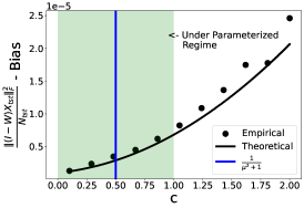
B.2 Generalization error - bias and variance

For both the data scaling and parameter scaling regimes, Figures 12 and 13 show the bias, $\|W_{opt}\|$ and the generalization error. Here we see that our estimate is accurate.

(a)

(b)

(c)

Figure 12: Figure showing the bias, $\|W_{opt}\|_{F}^{2}$, and the generalization error in the data scaling regime for $\mu=1$, $\sigma_{trn}=\sqrt{N_{trn}}$, and $\sigma_{tst}=\sqrt{N_{tst}}$. Here $d=1000$ and $N_{tst}=1000$. For each empirical data point, we ran at least 100 trials. More details can be found in Appendix D.

(a)

(b)

(c)

Figure 13: Figure showing the $\|W_{opt}\|_{F}^{2}$, and the generalization error in the parameter scaling regime for $\mu=1$, $\sigma_{trn}=\sqrt{N_{trn}}$, and $\sigma_{tst}=\sqrt{N_{tst}}$. Here $N_{trn}=1000$ and $N_{tst}=1000$. For each empirical data point, we ran at least 100 trials. More details can be found in Appendix D.

Appendix C Regularization

C.1 Optimal Value of $\mu$

(a)

(b)

Figure 14: Figure showing the generalization error versus $\mu$ for $\sigma_{trn}^{2}=N_{trn}$ and $\sigma_{tst}^{2}=N_{tst}$.

We now explore the effect of fixing $\sigma_{trn}$ and then changing $\mu$. Figure 14, shows a $U$ shaped curve for the generalization error versus $\mu$, suggesting that there is an optimal value of $\mu$, which should be used to minimize the generalization error.

(a)

(b)

(c)

Figure 15: Figure for the optimal value of $\mu$ versus for different values of $\sigma_{trn}$

Next, we compute the optimal value of $\mu$ using grid search and plot it against $c$. Figure 15 shows double descent for the optimal value of $\mu$ for small values of $\sigma_{trn}$. Thus for low SNR data we see double descent, but we do not for high SNR data.

(a)

(b)

Figure 16: Figure showing the generalization error versus $\mu$ for the optimal $\sigma_{trn}^{2}$ and $\sigma_{tst}^{2}=N_{tst}$.

Finally, for a given value of $\mu$ and $c$, we compute the optimal $\sigma_{trn}$. We then compute the generalization error (when using the optimal $\sigma_{trn}$) and plot the generalization error versus $\mu$ curve. Figure 16 displays a very different trend from Figure 14. Instead of having a $U$-shaped curve, we have a monotonically decreasing generalization error curve. This suggests that we can improve generalization by using higher-quality training while compensating for this by increasing the amount of ridge regularization.

(a)

(b)

Figure 17: Trade-off between the regularizers. The left column is the optimal $\sigma_{trn}$, the central column is the optimal $\mu$, and the right column is the generalization error for these parameter restrictions

C.2 Trade-off in Parameter Scaling Regime

Here we look at the trade-off between $\sigma_{trn}$ and $\mu$ for the parameter scaling regime. We again see that the model implicitly prefers regularizing via ridge regularization and not via input data noise regularizer.

Appendix D Experiments

All experiments were conducted using Pytorch and run on Google Colab using an A100 GPU. For each empirical data point, we did at least 100 trials. The maximum number of trials for any experiment was 20000 trials.

For each configuration of the parameters, $N_{trn},N_{tst},d,\sigma_{trn},\sigma_{tst}$, and $\mu$. For each trial, we sampled $u,v_{trn},v_{tst}$ uniformly at random from the appropriate dimensional sphere. We also sampled new training and test noise for each trial.

For the data scaling regime, we kept $d=1000$ and for the parameter scaling regime, we kept $N_{trn}=1000$. For all experiments, $N_{tst}=1000$.

Appendix E Technical Assumption on $\mu$

Notice that we had this assumption that $p(\mu)<0$. We compute $p(\mu)$ for a million equally spaced points in $(0,100]$ and see that $p(\mu)<0$. Here we use Mpmath with a precision of 1000. The result is shown in Figure 18. Hence we see that the assumption is satisfied for $\mu\in(0,100]$.

Figure 18: Figure showing the value of $p(\mu)$

References

- [1] Manfred Opper and Wolfgang Kinzel “Statistical Mechanics of Generalization” In Models of Neural Networks III: Association, Generalization, and Representation, 1996
- [2] Mikhail Belkin, Daniel J. Hsu, Siyuan Ma and Soumik Mandal “Reconciling Modern Machine-Learning Practice and the Classical Bias–Variance Trade-off” In Proceedings of the National Academy of Sciences, 2019
- [3] Madhu S. Advani, Andrew M. Saxe and Haim Sompolinsky “High-dimensional Dynamics of Generalization Error in Neural Networks” In Neural Networks, 2020
- [4] Chen Cheng and Andrea Montanari “Dimension Free Ridge Regression” In arXiv preprint arXiv:2210.08571, 2022
- [5] Edgar Dobriban and Stefan Wager “High-dimensional asymptotics of prediction: Ridge regression and classification” In The Annals of Statistics, 2018
- [6] Gabriel Mel and Surya Ganguli “A Theory of High Dimensional Regression with Arbitrary Correlations Between Input Features and Target Functions: Sample Complexity, Multiple Descent Curves and a Hierarchy of Phase Transitions” In Proceedings of the 38th International Conference on Machine Learning, 2021
- [7] Vidya Muthukumar, Kailas Vodrahalli and Anant Sahai “Harmless Interpolation of Noisy Data in Regression” In 2019 IEEE International Symposium on Information Theory (ISIT), 2019
- [8] Peter Bartlett, Philip M. Long, Gábor Lugosi and Alexander Tsigler “Benign Overfitting in Linear Regression” In Proceedings of the National Academy of Sciences, 2020
- [9] Mikhail Belkin, Daniel J. Hsu and Ji Xu “Two Models of Double Descent for Weak Features” In SIAM Journal on Mathematics of Data Science, 2020
- [10] Michal Derezinski, Feynman T Liang and Michael W Mahoney “Exact Expressions for Double Descent and Implicit Regularization Via Surrogate Random Design” In Advances in Neural Information Processing Systems, 2020
- [11] Trevor Hastie, Andrea Montanari, Saharon Rosset and Ryan J. Tibshirani “Surprises in High-Dimensional Ridgeless Least Squares Interpolation” In The Annals of Statistics, 2022
- [12] Bruno Loureiro et al. “Learning Gaussian Mixtures with Generalized Linear Models: Precise Asymptotics in High-dimensions” In Advances in Neural Information Processing Systems, 2021
- [13] Song Mei, Theodor Misiakiewicz and Andrea Montanari “Generalization Error of Random Feature and Kernel Methods: Hypercontractivity and Kernel Matrix Concentration” In Applied and Computational Harmonic Analysis, 2022
- [14] Song Mei and Andrea Montanari “The Generalization Error of Random Features Regression: Precise Asymptotics and the Double Descent Curve” In Communications on Pure and Applied Mathematics 75, 2021
- [15] Song Mei, Andrea Montanari and Phan-Minh Nguyen “A Mean Field View of the Landscape of Two-layer Neural Networks” In Proceedings of the National Academy of Sciences of the United States of America, 2018
- [16] Nilesh Tripuraneni, Ben Adlam and Jeffrey Pennington “Covariate Shift in High-Dimensional Random Feature Regression” In ArXiv, 2021
- [17] Federica Gerace et al. “Generalisation Error in Learning with Random Features and the Hidden Manifold Model” In Proceedings of the 37th International Conference on Machine Learning, 2020
- [18] Blake Woodworth et al. “Kernel and Rich Regimes in Overparametrized Models” In Proceedings of Thirty Third Conference on Learning Theory, 2020
- [19] Bruno Loureiro et al. “Learning Curves of Generic Features Maps for Realistic Datasets with a Teacher-Student Model” In NeurIPS, 2021
- [20] Behrooz Ghorbani, Song Mei, Theodor Misiakiewicz and Andrea Montanari “Limitations of Lazy Training of Two-layers Neural Network” In Advances in Neural Information Processing Systems, 2019
- [21] Behrooz Ghorbani, Song Mei, Theodor Misiakiewicz and Andrea Montanari “When Do Neural Networks Outperform Kernel Methods?” In Advances in Neural Information Processing Systems, 2020
- [22] Ben Adlam and Jeffrey Pennington “The Neural Tangent Kernel in High Dimensions: Triple Descent and a Multi-Scale Theory of Generalization” In International Conference on Machine Learning, 2020
- [23] Stéphane d’Ascoli, Levent Sagun and Giulio Biroli “Triple Descent and the Two Kinds of Overfitting: Where and Why Do They Appear?” In Advances in Neural Information Processing Systems, 2020
- [24] Preetum Nakkiran, Prayaag Venkat, Sham M. Kakade and Tengyu Ma “Optimal Regularization can Mitigate Double Descent” In International Conference on Learning Representations, 2020
- [25] Behrooz Ghorbani, Song Mei, Theodor Misiakiewicz and Andrea Montanari “Linearized Two-layers Neural Networks in High Dimension” In The Annals of Statistics, 2021
- [26] Lin Chen, Yifei Min, Mikhail Belkin and Amin Karbasi “Multiple Descent: Design Your Own Generalization Curve” In Advances in Neural Information Processing Systems, 2021
- [27] Scott Fortmann-Roe “Understanding the Bias-Variance Tradeoff”, 2012 URL: http://scott.fortmann-roe.com/docs/BiasVariance.html
- [28] Alnur Ali, Edgar Dobriban and Ryan J. Tibshirani “The Implicit Regularization of Stochastic Gradient Flow for Least Squares” In International Conference on Machine Learning, 2020
- [29] Arthur Jacot et al. “Implicit Regularization of Random Feature Models” In Proceedings of the 37th International Conference on Machine Learning, 2020
- [30] Ohad Shamir “The Implicit Bias of Benign Overfitting” In Proceedings of Thirty Fifth Conference on Learning Theory, 2022
- [31] Behnam Neyshabur “Implicit Regularization in Deep Learning” In ArXiv abs/1709.01953, 2017
- [32] Behnam Neyshabur, Srinadh Bhojanapalli, David Mcallester and Nati Srebro “Exploring Generalization in Deep Learning” In Advances in Neural Information Processing Systems, 2017
- [33] Behnam Neyshabur, Ryota Tomioka and Nathan Srebro “In Search of the Real Inductive Bias: On the Role of Implicit Regularization in Deep Learning” In CoRR abs/1412.6614, 2015
- [34] Rishi Sonthalia and Raj Rao Nadakuditi “Training Data Size Induced Double Descent For Denoising Feedforward Neural Networks and the Role of Training Noise” In Transactions on Machine Learning Research, 2023
- [35] Dmitry Kobak, Jonathan Lomond and Benoit Sanchez “The Optimal Ridge Penalty for Real-World High-Dimensional Data Can Be Zero or Negative Due to the Implicit Ridge Regularization” In Journal of Machine Learning Research, 2022
- [36] Fatih Furkan Yilmaz and Reinhard Heckel “Regularization-Wise Double Descent: Why it Occurs and How to Eliminate it” In IEEE International Symposium on Information Theory, 2022
- [37] Ningyuan Huang, David W. Hogg and Soledad Villar “Dimensionality Reduction, Regularization, and Generalization in Overparameterized Regressions” In SIAM Journal on Mathematics of Data Science, 2022
- [38] Ji Xu and Daniel J Hsu “On the number of variables to use in principal component regression” In Advances in neural information processing systems, 2019
- [39] Denny Wu and Ji Xu “On the Optimal Weighted Regularization in Overparameterized Linear Regression” In Advances in Neural Information Processing Systems, 2020
- [40] Chinmaya Kausik, Kashvi Srivastava and Rishi Sonthalia “Generalization Error without Independence: Denoising, Linear Regression, and Transfer Learning”, 2023
- [41] Daniel Soudry, Elad Hoffer, Suriya Gunasekar and Nathan Srebro “The Implicit Bias of Gradient Descent on Separable Data” In Journal of Machine Learning Research 19, 2018
- [42] Ben Poole et al. “Exponential Expressivity in Deep Neural Networks Through Transient Chaos” In Advances in Neural Information Processing Systems, 2016
- [43] Yunwen Lei, Ting Hu and Ke Tang “Generalization Performance of Multi-Pass Stochastic Gradient Descent with Convex Loss Functions” In Journal of Machine Learning Research, 2022
- [44] Courtney Paquette, Elliot Paquette, Ben Adlam and Jeffrey Pennington “Homogenization of SGD in High-dimensions: Exact Dynamics and Generalization Properties”, 2022
- [45] Kaifeng Lyu and Jian Li “Gradient Descent Maximizes the Margin of Homogeneous Neural Networks” In International Conference on Learning Representations, 2020
- [46] Ziwei Ji and Matus Telgarsky “The Implicit Bias of Gradient Descent on Nonseparable Data” In Proceedings of the Thirty-Second Conference on Learning Theory, 2019
- [47] Benjamin Bowman and Guido Montúfar “Implicit Bias of MSE Gradient Optimization in Underparameterized Neural Networks” In International Conference on Learning Representations, 2022
- [48] Lénaïc Chizat and Francis Bach “Implicit Bias of Gradient Descent for Wide Two-Layer Neural Networks Trained with the Logistic Loss” In Proceedings of Thirty Third Conference on Learning Theory, 2020
- [49] Simon Du et al. “Gradient Descent Finds Global Minima of Deep Neural Networks” In Proceedings of the 36th International Conference on Machine Learning, 2019
- [50] Simon S. Du, Xiyu Zhai, Barnabas Poczos and Aarti Singh “Gradient Descent Provably Optimizes Over-parameterized Neural Networks” In International Conference on Learning Representations, 2019
- [51] Alnur Ali, J. Kolter and Ryan J. Tibshirani “A Continuous-Time View of Early Stopping for Least Squares Regression” In International Conference on Artificial Intelligence and Statistics, 2019
- [52] Courtney Paquette, Elliot Paquette, Ben Adlam and Jeffrey Pennington “Implicit Regularization or Implicit Conditioning? Exact Risk Trajectories of SGD in High Dimensions” In ArXiv abs/2206.07252, 2022
- [53] Chris M. Bishop “Training with Noise is Equivalent to Tikhonov Regularization” In Neural Computation, 1995
- [54] Alexander Camuto et al. “Explicit Regularisation in Gaussian Noise Injections” In Advances in Neural Information Processing Systems, 2020, pp. 16603–16614
- [55] KyungHyun Cho “Boltzmann Machines for Image Denoising” In Artificial Neural Networks and Machine Learning, 2013
- [56] Reinhard Heckel and Mahdi Soltanolkotabi “Denoising and Regularization via Exploiting the Structural Bias of Convolutional Generators” In International Conference on Learning Representations, 2020
- [57] Wei Hu, Zhiyuan Li and Dingli Yu “Simple and Effective Regularization Methods for Training on Noisily Labeled Data with Generalization Guarantee” In International Conference on Learning Representations, 2020
- [58] Arvind Neelakantan et al. “Adding Gradient Noise Improves Learning for Very Deep Networks” In ArXiv abs/1511.06807, 2015
- [59] Ting Chen, Simon Kornblith, Mohammad Norouzi and Geoffrey Hinton “A Simple Framework for Contrastive Learning of Visual Representations” In Proceedings of the 37th International Conference on Machine Learning, 2020
- [60] Pascal Vincent et al. “Stacked Denoising Autoencoders: Learning Useful Representations in a Deep Network with a Local Denoising Criterion” In Journal of Machine Learning Research, 2010
- [61] Ben Poole, Jascha Narain Sohl-Dickstein and Surya Ganguli “Analyzing Noise in Autoencoders and Deep Networks” In ArXiv, 2014
- [62] Nitish Srivastava et al. “Dropout: A Simple Way to Prevent Neural Networks from Overfitting” In Journal of Machine Learning Research, 2014
- [63] Aharon. Ben-Tal, Laurent E. Ghaoui and Arkadi Nemirovski “Robust Optimization”, Princeton Series in Applied Mathematics, 2009
- [64] Adnan Siraj Rakin, Zhezhi He and Deliang Fan “Parametric Noise Injection: Trainable Randomness to Improve Deep Neural Network Robustness Against Adversarial Attack” In 2019 IEEE/CVF Conference on Computer Vision and Pattern Recognition (CVPR), 2019
- [65] Dimitris Bertsimas, David Brown and Constatine Caramanis “Theory and Applications of Robust Optimization” In SIAM Review, 2011
- [66] Naveed Akhtar and Ajmal Mian “Threat of Adversarial Attacks on Deep Learning in Computer Vision: A Survey” In IEEE Access, 2018
- [67] Anirban Chakraborty et al. “A Survey on Adversarial Attacks and Defences” In CAAI Transactions on Intelligence Technology, 2018
- [68] Arnu Pretorius, Steve Kroon and Herman Kamper “Learning Dynamics of Linear Denoising Autoencoders” In International Conference on Machine Learning, 2018
- [69] Raj R. Nadakuditi “OptShrink: An Algorithm for Improved Low-Rank Signal Matrix Denoising by Optimal, Data-Driven Singular Value Shrinkage” In IEEE Transactions on Information Theory, 2014
- [70] Marc Lelarge and Léo Miolane “Fundamental Limits of Symmetric Low-Rank Matrix Estimation” In Proceedings of the 2017 Conference on Learning Theory, 2017
- [71] Thibault Lesieur, Florent Krzakala and Lenka Zdeborová “Constrained Low-Rank Matrix Estimation: Phase Transitions, Approximate Message Passing and Applications” In Journal of Statistical Mechanics: Theory and Experiment, 2017
- [72] Antoine Maillard, Florent Krzakala, Marc Mézard and Lenka Zdeborová “Perturbative Construction of Mean-Field Equations in Extensive-Rank Matrix Factorization and Denoising” In Journal of Statistical Mechanics: Theory and Experiment, 2022
- [73] Emanuele Troiani et al. “Optimal Denoising of Rotationally Invariant Rectangular Matrices” In ArXiv abs/2203.07752, 2022
- [74] Dominic Richards, Jaouad Mourtada and Lorenzo Rosasco “Asymptotics of Ridge (Less) Regression under General Source Condition” In International Conference on Artificial Intelligence and Statistics, 2021
- [75] Ali Rahimi and Benjamin Recht “Random Features for Large-Scale Kernel Machines” In Advances in Neural Information Processing Systems, 2007
- [76] Andrew Ng “CS229 Lecture notes” In CS229 Lecture notes, 2000
- [77] Carl D. Meyer “Generalized Inversion of Modified Matrices” In SIAM Journal on Applied Mathematics, 1973
- [78] Friedrich Götze and Alexander Tikhomirov “The Rate of Convergence for Spectra of GUE and LUE Matrix Ensembles” In Central European Journal of Mathematics, 2005
- [79] Friedrich Götze and Alexander Tikhomirov “Rate of Convergence to the Semi-Circular Law” In Probability Theory and Related Fields, 2003
- [80] Friedrich Götze and Alexander Tikhomirov “Rate of Convergence in Probability to the Marchenko-Pastur Law” In Bernoulli, 2004
- [81] Vladimir Marcenko and Leonid Pastur “DISTRIBUTION OF EIGENVALUES FOR SOME SETS OF RANDOM MATRICES” In Mathematics of The Ussr-sbornik, 1967
- [82] Z. Bai, Baiqi. Miao and Jian-Feng. Yao “Convergence Rates of Spectral Distributions of Large Sample Covariance Matrices” In SIAM Journal on Matrix Analysis and Applications, 2003