Optimal Linear Subspace Search: Learning to Construct Fast and High-Quality Schedulers for Diffusion Models

Abstract.

In recent years, diffusion models have become the most popular and powerful methods in the field of image synthesis, even rivaling human artists in artistic creativity. However, the key issue currently limiting the application of diffusion models is its extremely slow generation process. Although several methods were proposed to speed up the generation process, there still exists a trade-off between efficiency and quality. In this paper, we first provide a detailed theoretical and empirical analysis of the generation process of the diffusion models based on schedulers. We transform the designing problem of schedulers into the determination of several parameters, and further transform the accelerated generation process into an expansion process of the linear subspace. Based on these analyses, we consequently propose a novel method called Optimal Linear Subspace Search (OLSS), which accelerates the generation process by searching for the optimal approximation process of the complete generation process in the linear subspaces spanned by latent variables. OLSS is able to generate high-quality images with a very small number of steps. To demonstrate the effectiveness of our method, we conduct extensive comparative experiments on open-source diffusion models. Experimental results show that with a given number of steps, OLSS can significantly improve the quality of generated images. Using an NVIDIA A100 GPU, we make it possible to generate a high-quality image by Stable Diffusion within only one second without other optimization techniques.

1. Introduction

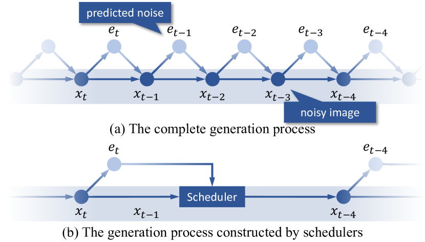
Figure 1. The complete generation process of diffusion models consists of hundreds of steps for gradual denoising. Diffusion schedulers speed up this process by skipping some steps but may make destructive changes to images.

In recent years, diffusion models (Ho et al., 2020; Nichol and Dhariwal, 2021; Song and Ermon, 2019) have become the most popular framework and have achieved impressive success in image synthesis (Feng et al., 2023; Ramesh et al., 2022; Saharia et al., 2022a). Unlike generative adversarial networks (GANs) (Goodfellow et al., 2020), diffusion models generate high-quality images without relying on adversarial training processes, and do not require careful hyperparameter tuning. In addition to image synthesis, diffusion models have also been applied to image super-resolution (Saharia et al., 2022b), music synthesis (Liu et al., 2022) and video synthesis (Esser et al., 2023). The research community and industry have witnessed the impressive effectiveness of diffusion models in generative tasks.

The major weakness of diffusion models, however, is the extremely slow sampling procedure, which limits their practicability (Yang et al., 2022). The diffusion model is a family of iterative generative models and typically requires hundreds to thousands of steps to generate content. The idea of diffusion models is inspired by the diffusion process in physics. In image synthesis, various levels of Gaussian noise are incrementally added to images (or latent variables corresponding to images) in a stepwise manner, while the model is trained to denoise the samples and reconstruct the original images. The generation process is the reverse process of diffusion process and both processes include the same time discretization steps to ensure consistency. The number of steps in the training stage required is usually very large to improve the image quality, making the generation process extremely slow.

To tackle the efficiency problem of diffusion models, existing studies proposed several types of methods. For instance, Salimans et al. (Salimans and Ho, 2021) proposed a distillation method that can reduce the number of sampling steps to half and can be applied repeatably to a model. By maximizing sample quality scores, DDSS (Watson et al., 2022) attempted to optimize fast samplers. However, these speedup methods require additional training, which makes it difficult to deploy them with limited computing resources. Another family of studies focused on designing a scheduler to control the generation process, including DDIM (Song et al., 2020), PNDM (Liu et al., 2021), DEIS (Zhang and Chen, 2022), etc. As shown in Figure 1, these schedulers can reduce the number of steps without training. However, when we use a small number of steps, these methods may introduce new noise and make destructive changes to images because of the inconsistency between the reconstructed generation process and the complete generation process. Hence we are still faced with a trade-off between the computing resource requirement and performance.

In order to speed up the generation process, we focus on devising an adaptive scheduler that requires only a little time for learning. In this paper, we first theoretically analyze the generation process of diffusion models. With the given steps, most of the existing schedulers (Song et al., 2020; Karras et al., 2022; Liu et al., 2021) generate the next sample in the linear subspace spanned by the previous samples and model outputs, thus the generation process is essentially the expansion process of linear subspaces. We also analyze the correlation of intermediate variables when generating images, and we observe that the model outputs contain redundant duplicate information at each step. Therefore, the number of steps must be reduced to prevent redundant calculation. In light of these analyses, we replace the coefficients in the iterative formula with trainable parameters to control the expansion of the linear subspaces, and then use simple least square methods (Björck, 1990; Kerr et al., 2009) to solve these parameters. Leveraging a path optimization algorithm, we further improve the performance by tuning the sampling steps. Path optimization and parameter solving can be performed within only a few minutes, thus it is easy to train and deploy. Our proposed scheduler, named Optimal Linear Subspace Search (OLSS), is designed to be lightweight and adaptive. We apply OLSS to several popular open-source diffusion models (Rombach et al., 2022) and compare the performance of OLSS with the state-of-the-art schedulers. Experimental results prove that the approximate generation process built by OLSS is an accurate approximation of the complete generation process. The source code of our proposed method has been released on GitHub. The main contribution of this paper includes:

• We theoretically and empirically analyze the generation process of diffusion models and model it as an expansion process of linear subspaces. The analysis provides valuable insights for researchers to design new diffusion schedulers.

• Based on our analysis, we propose a novel scheduler, OLSS, which is capable of finding the optimal path to approximate the complete generation process and generating high-quality images with a very small number of steps.

• Using several popular diffusion models, we benchmark OLSS against existing schedulers. The experimental results demonstrate that OLSS achieves the highest image quality with the same number of steps.

2. Related Work

2.1. Image Synthesis

Image synthesis is an important task and has been widely investigated. In the early years, GANs (Reed et al., 2016; Huang et al., 2017; Odena et al., 2017) are the most popular methods. By adversarial training a generator and a discriminator, we can obtain a network that can directly generate images. However, it is difficult to stabilize the training process (Salimans et al., 2016). Diffusion models overcome this issue by modeling the synthesis task as a Markovian diffusion process. Theoretically, diffusion models include Denoising Diffusion Probabilistic Models (Sohl-Dickstein et al., 2015), Score-Based Generative Models (Song and Ermon, 2019), etc. In recent years, Latent Diffusion (Rombach et al., 2022), a diffusion model architecture that denoises images in a latent space, became the most popular model architecture. Utilizing cross-attention (Vaswani et al., 2017) and classifier-free guidance (Ho and Salimans, 2021), Latent Diffusion is able to generate semantically meaningful images according to given prompts. Leveraging large-scale text-image datasets (Gu et al., 2022; Schuhmann et al., 2022), diffusion models with billions of parameters have achieved impressive success in text-to-image synthesis. Diffusion models are proven to outperform GANs in image quality (Dhariwal and Nichol, 2021), and are even competitive with human artists (Feng et al., 2023; Ramesh et al., 2022; Saharia et al., 2022a). However, the slow sampling procedure becomes a critical issue, limiting the practicability of diffusion models.

2.2. Efficient Sampling for Diffusion Models

The time consumed of generating an image using diffusion models is in direct proportion to the number of inference steps. To speed up the generation process, existing studies focus on reducing the number of inference steps. Specifically, some schedulers are proposed for controlling this denoising process. DDIM (Denoising Diffusion Implicit Models) (Song et al., 2020) is a straightforward scheduler that converts the stochastic process to a deterministic process and skips some steps. Some numerical ODE algorithms (Butcher, 2000; Karras et al., 2022) are also introduced to improve efficiency. Liu et al. (Liu et al., 2021) pointed out that numerical ODE methods may introduce additional noise and are therefore less efficient than DDIM with only a small number of steps. To overcome this pitfall, they modified the iterative formula and improved their effectiveness. DEIS (Diffusion Exponential Integrator Sampler) (Zhang and Chen, 2022), another study based on ODE, stabilizes the approximated generation process leveraging an exponential integrator and a semilinear structure. DPM-Solver (Lu et al., 2022a) made further refinements by calculating a part of the solution analytically. Recently, an enhanced version (Lu et al., 2022b) of DPM-Solver adopted thresholding methods and achieved state-of-the-art performance.

3. Methodology

3.1. Review of Diffusion Models

Different from GAN-based generative models, diffusion-based models require multi-step inference. The iterative generation process significantly increases the computation time. In the training stage, the number of steps may be very large. For example, the number of steps in Stable Diffusion (Rombach et al., 2022) while training is $1000$.

In the complete generation process, starting from random Gaussian noise $\boldsymbol{x}_{T}$, we need to calculate $\boldsymbol{x}_{T-1},\dots,\boldsymbol{x}_{0}$ step by step, where $T$ is the total number of steps. At each step $t$, the diffusion model $\epsilon_{\theta}$ takes $\boldsymbol{x}_{t}$ as input and output $\boldsymbol{e}_{t}=\epsilon_{\theta}(\boldsymbol{x}_{t},t)$. We obtain $\boldsymbol{x}_{t-1}$ via:

(1) $$\begin{split}\boldsymbol{x}_{t-1}=&\sqrt{\alpha_{t-1}}\underbrace{\left(\frac{\boldsymbol{x}_{t}-\sqrt{1-\alpha_{t}}\boldsymbol{e}_{t}}{\sqrt{\alpha_{t}}}\right)}_{\text{predicted }\boldsymbol{x}_{0}}\\ &+\underbrace{\sqrt{1-\alpha_{t-1}-\sigma_{t}^{2}}\boldsymbol{e}_{t}}_{\text{direction pointing to }\boldsymbol{x}_{t}}+\underbrace{\sigma_{t}\boldsymbol{\epsilon}_{t}}_{\text{random noise}},\end{split}$$

where $\alpha_{t},\sigma_{t}$ are hyper-parameters used for training. Note that $\sigma_{t}\boldsymbol{\epsilon}_{t}$ is the additional random noise to increase the diversity of generated results. In DDIM (Song et al., 2020), $\sigma_{t}$ is set to $0$, making this process deterministic given $\boldsymbol{x}_{T}$.

To reduce the steps, in most existing schedulers, a few steps $t(1),\dots,t(n)$ are selected as a sub-sequence of $\{T,T-1,\dots,0\}$, and the scheduler only calls the model to calculate $\boldsymbol{e}_{t(i)}$ at these $n$ steps. For example, DDIM directly transfers Formula (1) to an $n$-step generation process:

(2) $$\begin{split}\boldsymbol{x}_{t(i+1)}=&\sqrt{\alpha_{t(i+1)}}\left(\frac{\boldsymbol{x}_{t(i)}-\sqrt{1-\alpha_{t(i)}}\boldsymbol{e}_{t(i)}}{\sqrt{\alpha_{t(i)}}}\right)\\ &+\sqrt{1-\alpha_{t(i+1)}}\boldsymbol{e}_{t(i)}.\end{split}$$

The final tensor $\boldsymbol{x}_{0}$ obtained by DDIM is an approximate result of that in the complete generation process. Another study (Karras et al., 2022) focuses on modeling the generation process as an ordinary differential equation (ODE) (Butcher, 2000). Consequently, forward Euler, a general numerical ODE algorithm, can be employed to calculate the numerical solution of $\boldsymbol{x}_{0}$:

(3) $$\boldsymbol{x}_{t(i+1)}=\boldsymbol{x}_{t(i)}+\Big{(}t(i+1)-t(i)\Big{)}\frac{\mathrm{d}\boldsymbol{x}_{t(i)}}{\mathrm{d}t(i)},$$

where

(4) $$\frac{\mathrm{d}\boldsymbol{x}_{t}}{\mathrm{d}t}=-\frac{\mathrm{d}\alpha_{t}}{\mathrm{d}t}\left(\frac{\boldsymbol{x}_{t}}{2\alpha_{t}}-\frac{\boldsymbol{e}_{t}}{2\alpha_{t}\sqrt{1-\alpha_{t}}}\right).$$

PNDM (Liu et al., 2021) is another ODE-based scheduler. It leverages Linear Multi-Step Method and constructs a pseudo-numerical method. We simplify the iterative formula of PNDM as:

(5) $$\boldsymbol{x}_{t(i+1)}=\frac{\sqrt{\alpha_{t(i+1)}}}{\sqrt{\alpha_{t(i)}}}\boldsymbol{x}_{t(i)}-\frac{1}{\sqrt{\alpha_{t(i)}}}\alpha_{t(i)}^{\prime}\boldsymbol{e}_{t(i)}^{\prime},$$

where

(6) $$\boldsymbol{e}_{t(i)}^{\prime}=\frac{1}{24}(55\boldsymbol{e}_{t(i)}-59\boldsymbol{e}_{t(i-1)}+37\boldsymbol{e}_{t(i-2)}-9\boldsymbol{e}_{t(i-3)}),$$

(7) $$\alpha_{t(i)}^{\prime}=\frac{\alpha_{t(i+1)}-\alpha_{t(i)}}{\sqrt{(1-\alpha_{t(i+1)})\alpha_{t(i)}}+\sqrt{(1-\alpha_{t(i)})\alpha_{t(i+1)}}}.$$

In DDIM (2) and forward Euler (3), $\boldsymbol{x}_{t(i+1)}$ is a linear combination of $\{\boldsymbol{x}_{t(i)},\boldsymbol{e}_{t(i)}\}$. In PNDM (5), $\boldsymbol{x}_{t(i+1)}$ is a linear combination of $\{\boldsymbol{x}_{t(i)},\boldsymbol{e}_{t(i)},\boldsymbol{e}_{t(i-1)},\boldsymbol{e}_{t(i-2)},\boldsymbol{e}_{t(i-3)}\}$. Generally, all these schedulers satisfy

(8) $$\boldsymbol{x}_{t(i+1)}\in\text{span}\{\boldsymbol{x}_{t(i)},\boldsymbol{e}_{t(1)},\boldsymbol{\dots},\boldsymbol{e}_{t(i)}\}.$$

Recursively, we can easily prove that

(9) $$\boldsymbol{x}_{t(i+1)}\in\text{span}\{\boldsymbol{x}_{t(1)},\boldsymbol{e}_{t(1)},\boldsymbol{\dots},\boldsymbol{e}_{t(i)}\}.$$

Therefore, the generation process is the expansion process of a linear subspace. This linear subspace is spanned by the initial Gaussian noise and the previous model outputs. At each step, we obtain the model output and add it to the vector set. The core issue of designing a scheduler is to determine the coefficients in the iterative formula. The number of non-zero coefficients does not exceed $\frac{1}{2}n^{2}+\frac{3}{2}n$.

3.2. Empirical Analysis of Generation Process

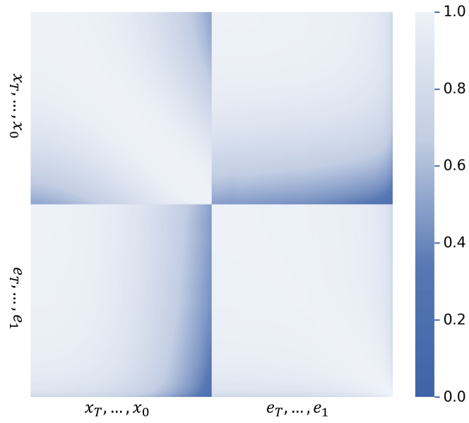
Figure 2. The heat map of the correlation coefficients of latent variables, which records the whole generation process.

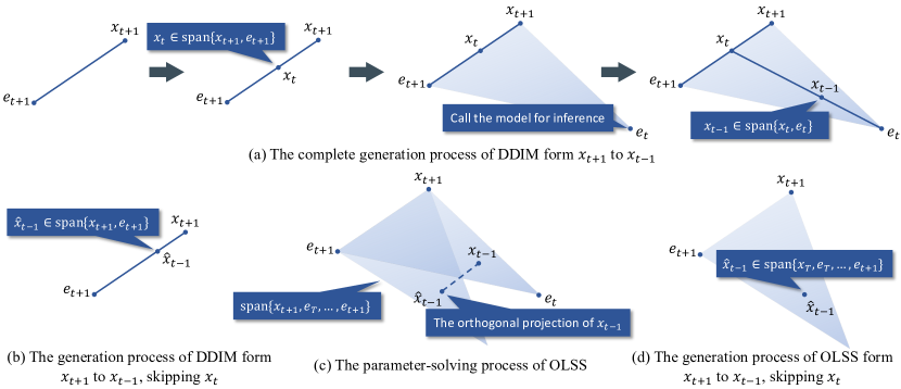
Figure 3. An interpretation of OLSS. (a) In the complete generation process of DDIM from $\boldsymbol{x}_{t+1}$ to $\boldsymbol{x}_{t-1}$, the scheduler first computes $\boldsymbol{x}_{t}\in\text{span}\{\boldsymbol{x}_{t+1},\boldsymbol{e}_{t+1}\}$ and then computes $\boldsymbol{x}_{t-1}\in\text{span}\{\boldsymbol{x}_{t},\boldsymbol{e}_{t}\}$. We have $\boldsymbol{x}_{t-1}\in\text{span}\{\boldsymbol{x}_{t+1},\boldsymbol{e}_{t+1},\boldsymbol{e}_{t}\}$. (b) If we use DDIM to skip $\boldsymbol{x}_{t}$, the scheduler will compute $\hat{\boldsymbol{x}}_{t-1}\in\text{span}\{\boldsymbol{x}_{t+1},\boldsymbol{e}_{t+1}\}$ using the iterative Formula (2). (c) If we use OLSS to skip $\boldsymbol{x}_{t}$, we use the orthogonal projection of $\boldsymbol{x}_{t-1}$ in $\text{span}\{\boldsymbol{x}_{t+1},\boldsymbol{e}_{T},\dots,\boldsymbol{e}_{t+1}\}$ as the estimation of $\boldsymbol{x}_{t-1}$. In the parameter-solving process, we compute the orthogonal projection matrix and construct the new iterative formula. (d) The linear subspace spanned by $\{\boldsymbol{x}_{t+1},\boldsymbol{e}_{T},\dots,\boldsymbol{e}_{t+1}\}$ is equivalent to the linear subspace spanned by $\{\boldsymbol{x}_{T},\boldsymbol{e}_{T},\dots,\boldsymbol{e}_{t+1}\}$. In the generation process of OLSS, we directly compute $\hat{\boldsymbol{x}}_{t-1}\in\text{span}\{\boldsymbol{x}_{T},\boldsymbol{e}_{T},\dots,\boldsymbol{e}_{t+1}\}$. Compared with DDIM, the estimation of $\boldsymbol{x}_{t-1}$ is in a higher dimensional linear subspace, thus it is more accurate.

To empirically analyze what happens in the whole generation process, we use Stable Diffusion to generate several images and store the latent variables, including $\boldsymbol{x}_{T},\dots,\boldsymbol{x}_{0},\boldsymbol{e}_{T},\dots,\boldsymbol{e}_{1}$. As shown in Figure 2, we plot a heat map showing the correlation coefficients between these variables. We have the following findings:

1. $\boldsymbol{x}_{t}$ is similar to that in neighboring steps and differs from that in non-neighboring steps. As the denoising process proceeds, $\boldsymbol{x}_{t}$ is updated continuously.

2. The correlation between $\boldsymbol{x}_{t}$ and the predicted noise $\boldsymbol{e}_{t}$ is strong in the beginning and becomes weak in the end. The reason is that $\boldsymbol{x}_{t}$ consists of little noise in the last few steps.

3. The correlation between $\boldsymbol{e}_{T},\dots,\boldsymbol{e}_{1}$ is significantly strong, indicating that the outputs of the model contain redundant duplicate information.

3.3. Constructing a Faster Scheduler

On the basis of existing schedulers and our analysis, we propose OLSS, a new diffusion scheduler. In this method, we first run the complete generation process to catch the intermediate variables and then construct an approximate process using these variables, instead of leveraging mathematical theories to design a new iterative formula.

Assume that we have selected $n$ steps $\{t(1),\dots,t(n)\}$, which is a sub-sequence of $\{T,T-1,\dots,0\}$ with $t(1)=T$. Calling the diffusion model for inference is only allowed at these $n$ steps. At the $i$-th step, we have obtained intermediate variables $\boldsymbol{x}_{t(1)},\dots,\boldsymbol{x}_{t(i)}$ and $\boldsymbol{e}_{t(1)},\dots,\boldsymbol{e}_{t(i)}$. In the complete generation process, it needs to call the model for $t(i+1)-t(i)-1$ times. To reduce time consumption, we naturally come up with a naive method. As we mentioned in Section 3.2, the correlation between $\boldsymbol{e}_{T},\dots,\boldsymbol{e}_{1}$ is significantly strong, thus we can estimate the model’s output $\boldsymbol{e}_{t(i)-1}$ using a simple linear model trained with intermediate variables. Formally, let

(10) $$\hat{\boldsymbol{e}}_{t(i)-1}=\mathop{\arg\min}_{\boldsymbol{e}\in\mathcal{E}}||\boldsymbol{e}-\boldsymbol{e}_{t(i)-1}||_{2}^{2},$$

where the feasible region is

(11) $$\mathcal{E}=\text{span}\{\boldsymbol{x}_{t(1)},\boldsymbol{e}_{t(1)},\dots,\boldsymbol{e}_{t(i)}\}.$$

In other words, we use the orthogonal projection of $\boldsymbol{e}_{t(i)-1}$ in $\mathcal{E}$ as the estimation of $\boldsymbol{e}_{t(i)-1}$. Similarly, we can obtain all estimated intermediate variables in the missing steps before $t(i+1)$ and finally calculate $\hat{\boldsymbol{x}}_{t(i+1)}$. According to Equations (9, 10, 11), it is obvious to see the estimated $\boldsymbol{x}_{t(i+1)}$ still satisfies Equation (9). However, note that the estimation may have non-negligible errors and the errors are accumulated into subsequent steps. To address this issue, we design a simplified end-to-end method that directly estimates $\boldsymbol{x}_{t(i+1)}$. The simplified method only contains one linear model, containing $i+1$ coefficients $w_{i,0},w_{i,1},\dots,w_{i,i}$. The estimated $\boldsymbol{x}_{t(i+1)}$ is formulated as:

(12) $$\hat{\boldsymbol{x}}_{t(i+1)}=w_{i,0}\boldsymbol{x}_{t(1)}+\sum_{j=1}^{i}w_{i,j}\boldsymbol{e}_{t(j)}.$$

The decision space in this simplified method is consistent with the naive method mentioned above. Leveraging least square methods (Björck, 1990), we can easily minimize the mean square error $||\hat{\boldsymbol{x}}_{t(i+1)}-\boldsymbol{x}_{t(i+1)}||_{2}^{2}$. Note that we use only $\boldsymbol{x}_{t(1)}$ (i.e., $\boldsymbol{x}_{T}$) instead of all intermediate variables $\{\boldsymbol{x}_{t(1)},\dots,\boldsymbol{x}_{t(i)}\}$ in Equation (12), because $\{\boldsymbol{x}_{t(1)},\boldsymbol{e}_{t(1)},\dots,\boldsymbol{e}_{t(i)}\}$ is a linearly independent set and the other vectors $\{\boldsymbol{x}_{t(2)},\dots,\boldsymbol{x}_{t(i)}\}$ can be linearly represented by these vectors. Additionally, the linear independence makes it easier to solve the least squares problem using QR-decomposition algorithms (Kerr et al., 2009), which is faster and more numerically stable than directly computing the pseudo-inverse matrix (Regalia, 1993).

Algorithm 1 Step Searching with error upper bound $D$

1:  Input: Error upper bound $D$

2:  Input: Previous steps $\{t(1),\dots,t(i)\}$

3:  $t_{l}=t(i),t_{r}=0$

4:  while $t_{l}>t_{r}$ do

5:     $t_{m}=\lfloor\frac{t_{l}+t_{r}}{2}\rfloor$

6:     if $d(t(1),\dots,t(i),t_{m})>D$ then

7:        $t_{r}=t_{m}+1$

8:     else

9:        $t_{l}=t_{m}$

10:     end if

11:  end while

12:  $t(i+1)=t_{l}$

13:  return  $t(i+1)$

Algorithm 2 Path searching with error upper bound $D$

1:  Input: Error upper bound $D$

2:  $t(1)=T$

3:  for $i=1,2,\dots,n$ do

4:     Find $t(i+1)$ using Algorithm 1

5:     if $t(i+1)$ does not exist then

6:        return  None

7:     end if

8:  end for

9:  if $t(n+1)>0$ then

10:     return  None

11:  else

12:     return  $\{t(1),t(2),\dots,t(n)\}$

13:  end if

Algorithm 3 Path optimization

1:  Input: The required absolute error $\epsilon$ of optimal error limit

2:  $D_{l}=0$

3:  $D_{r}=10$ (a sufficiently large value)

4:  while $D_{r}-D_{l}>\epsilon$ do

5:     $D_{m}=\frac{t_{l}+t_{r}}{2}$

6:     Find a path $\mathcal{T}$ with error limit $D_{m}$ using Algorithm 2

7:     if $\mathcal{T}$ is not None then

8:        $D_{r}=D_{m}$

9:     else

10:        $D_{l}=D_{m}$

11:     end if

12:  end while

13:  Find a path $\mathcal{T}$ with error limit $D_{r}$

14:  return  $\mathcal{T}$

We provide an interpretation of OLSS in Figure 3. When we skip $\boldsymbol{x}_{t}$, OLSS computes an estimation of $\boldsymbol{x}_{t-1}$ in the linear subspace spanned by the initial Gaussian noise and the previous model outputs. Essentially, this estimation is the orthogonal projection of $\boldsymbol{x}_{t-1}$ in the linear subspace. Each time we call the model for inference, the linear subspace is expanded by the predicted noise. Therefore, the generation process is the expansion process of the linear subspace.

3.4. Searching for the Optimal Path

Another problem to be addressed is how to select the $n$ steps $\{t(1),\dots,t(n)\}$. In Section 3.2, we observe that the correlation between $\boldsymbol{x}_{t}$ and $\boldsymbol{e}_{t}$ is different at each step, indicating that the difficulty level of generating low-error $\boldsymbol{x}_{t}$ is also varied. In most existing schedulers, these steps are selected in $\{T,T-1,\dots,0\}$ with equal intervals. For example, in PNDM, Equation (6) comes from the Linear Multi-Step Method, which enforces that the steps must be uniformly selected. However, there is no restriction on the selection of steps in our method. We can search for the optimal path to generate high-quality images.

For convenience, we use $d(t(1),\dots,t(i+1))$ to denote the distance from $\boldsymbol{x}_{t(i+1)}$ to its orthogonal projection in the linear subspace spanned by $\{\boldsymbol{x}_{t(1)},\boldsymbol{e}_{t(1)},\dots,\boldsymbol{e}_{t(i)}\}$ (i.e., the error of $\hat{\boldsymbol{x}}_{t(i+1)}$). We add an additional step $t(n+1)=0$. To find the optimal path $\mathcal{T}=\{t(1),\dots,t(n+1)\}$, we formulate the path optimization problem as:

(13) $$\mathcal{T}=\mathop{\arg\min}_{t(1),\dots,t(n+1)}\max_{i=1}^{n}d(t(1),\dots,t(i+1)),$$

(14) $$\text{s.t. }T=t(1)\geq t(2)\geq\dots\geq t(n)\geq t(n+1)=0.$$

We intend to minimize the largest error in the $n$ steps. Setting an error upper bound $D$, we hope the error of every step does not exceed $D$. Such a path always exists if $D$ is sufficiently large, thus we can use a binary search algorithm to compute the minimal error upper bound $D$ when a path exists. The pseudo-code is presented in Algorithm 3. In this binary search algorithm, we have to design another algorithm to check whether the path with the error upper bound $D$ exists.

According to the conclusions in Section 3.2, the more steps we skip, the larger errors we have. However, if we only skip a small number of steps to reduce the error, the path will not end at $0$ within $n$ steps. Therefore, we use another binary search algorithm to search for the next step based on a greedy strategy. By skipping more steps as possible, we can find a path with the error upper bound $D$ if it exists. The pseudo-code of finding the next step with error limitation is presented in Algorithm 1, and the pseudo-code of finding the path is presented in Algorithm 2.

The whole path optimization algorithm includes three loops. From inner to outer, the pseudo-codes of the three loops are presented in Algorithm 1-3. The first one is to find the next step with an error limitation. The second one is to check if such a path exists. Algorithm 2 will return the path to Algorithm 3 if it exists. The third one is to find the minimal error upper bound. Leveraging the whole path optimization algorithm, we obtain the optimal path for constructing the generation process.

3.5. Efficiency Analysis

We analyze the time complexity of constructing an OLSS scheduler. The most time-consuming component is solving the least square problem. We need to solve the least square problem $\mathcal{O}(n)$ times if the path is fixed, and $\mathcal{O}(n\log\frac{1}{\epsilon}\log T)$ times to perform path optimization, where $\epsilon$ is the absolute error of optimal $D$. Empirically, when we use OLSS to improve the efficiency of Stable Diffusion, usually a few minutes of computation on the CPU is sufficient to compute the optimal path and solve all the parameters $\{w_{i,j}\}$ after all the required intermediate variables are collected from the complete generation process. In the inference phase, the computation on schedulers is negligible compared to the computation on the models. The total time consumed of generating an image is in direct proportion to the number of steps.

4. Experiments

To demonstrate the effectiveness of OLSS, we conduct comparative experiments. We further investigate the factors that affect the quality of images generated by OLSS.

4.1. Comparison of Diffusion Schedulers

We compare OLSS with $7$ baseline schedulers, including its variant OLSS-P and $6$ existing schedulers. 1) OLSS-P: A variant of our proposed OLSS that selects the steps $\{t(1),\dots,t(n)\}$ uniformly instead of using the path optimization algorithm. 2) DDIM (Song et al., 2020): A straightforward method that directly skips some steps in the generation process. It has been widely used in many diffusion models. 3) Euler (Karras et al., 2022): An algorithm of calculating ODEs’ numerical solution. We follow the implementation of k-diffusion and use the ancestral sampling version. 4) PNDM (Liu et al., 2021): An pseudo numerical method that improves the performance of Linear Multi-Step method. 5) DEIS (Zhang and Chen, 2022): A fast high-order solver designed for diffusion models. It consists of an exponential integrator and a semi-linear structure. 6) DPM-Solver (Lu et al., 2022a): A high-order method that analytically computes the linear part of the latent variables. 7) DPM-Solver++ (Lu et al., 2022b): An enhanced scheduler based on DPM-Solver. It solves ODE with a data prediction model and uses thresholding methods. DPM-Solver++ is the most recent state-of-the-art scheduler.

4.1.1. Experimental Settings

Table 1. The FID $\downarrow$ scores between diffusion schedulers with different steps. The best results are in bold, and the second best are underscored. ${\dagger}$: the generation result of 1000-step DDIM is the most high-quality irrespective of the computational efficiency.

Model	Steps / Scheduler		100 Steps						1000 Steps†
			DDIM	Euler	PNDM	DEIS	DPM -Solver	DPM -Solver++	DDIM
Stable Diffusion ($512\times 512$)	5 Steps	DDIM	82.62	78.14	84.40	84.91	85.00	85.24	84.55
		Euler	132.19	111.18	134.62	135.06	135.28	135.72	134.28
		PNDM	75.53	89.53	74.29	75.50	75.31	75.13	75.41
		DEIS	56.31	55.89	58.44	58.03	58.21	58.54	57.68
		DPM-Solver	55.39	55.94	57.49	57.09	57.27	57.59	56.76
		DPM-Solver++	54.78	56.11	56.82	56.41	56.59	56.91	56.08
		OLSS-P	48.67	61.27	48.62	48.80	48.77	48.72	48.94
		OLSS	48.34	61.11	48.40	48.61	48.60	48.57	48.79
	10 Steps	DDIM	52.52	59.87	53.71	54.37	54.46	54.66	54.13
		Euler	79.63	60.04	81.97	81.70	81.91	82.33	81.32
		PNDM	55.77	72.31	54.84	56.01	55.88	55.77	56.03
		DEIS	39.11	55.07	41.75	40.96	41.13	41.40	40.97
		DPM-Solver	38.93	55.33	41.53	40.75	40.92	41.17	40.73
		DPM-Solver++	38.42	55.72	41.06	40.17	40.33	40.59	40.02
		OLSS-P	37.33	59.28	38.64	38.36	38.36	38.38	38.60
		OLSS	36.46	58.09	37.68	37.66	37.66	37.67	37.79
	20 Steps	DDIM	38.04	57.14	39.07	40.90	40.99	41.17	41.13
		Euler	65.38	49.92	67.18	66.85	67.05	67.39	66.32
		PNDM	37.26	60.57	35.55	38.38	38.39	38.42	38.55
		DEIS	23.37	58.88	28.64	25.87	25.91	25.99	26.28
		DPM-Solver	24.38	60.03	28.73	26.16	26.12	26.08	26.72
		DPM-Solver++	26.21	61.43	29.61	27.31	27.20	27.08	27.94
		OLSS-P	22.91	58.96	28.20	25.02	25.04	25.11	25.42
		OLSS	20.78	58.71	27.26	22.98	23.04	23.09	23.23
Stable Diffusion 2 ($768\times 768$)	5 Steps	DDIM	93.50	80.83	95.12	98.10	98.16	98.38	97.62
		Euler	170.79	119.12	173.09	175.24	175.28	175.51	174.43
		PNDM	105.08	99.88	105.82	108.61	108.54	108.67	108.28
		DEIS	55.88	58.62	57.30	59.04	59.20	59.50	58.65
		DPM-Solver	54.90	58.77	56.31	58.02	58.18	58.48	57.63
		DPM-Solver++	54.25	59.13	55.67	57.30	57.45	57.75	56.91
		OLSS-P	50.03	65.20	51.38	51.95	51.87	51.83	51.95
		OLSS	49.18	64.89	50.64	51.17	51.11	51.07	51.11
	10 Steps	DDIM	55.32	62.05	56.01	58.74	58.83	59.03	58.47
		Euler	96.86	61.75	98.57	100.88	100.99	101.26	100.15
		PNDM	56.44	64.58	56.94	59.52	59.62	59.81	59.28
		DEIS	39.83	60.85	42.11	42.59	42.74	43.02	42.33
		DPM-Solver	39.70	61.22	41.93	42.41	42.56	42.81	42.17
		DPM-Solver++	39.40	61.81	41.62	41.89	42.04	42.30	41.66
		OLSS-P	38.39	64.21	40.46	40.70	40.70	40.74	40.63
		OLSS	38.10	63.81	40.15	40.46	40.48	40.54	40.45
	20 Steps	DDIM	40.19	61.44	40.83	44.12	44.25	44.42	44.03
		Euler	74.53	48.51	76.08	77.80	77.94	78.18	77.24
		PNDM	40.93	62.20	40.26	44.19	44.35	44.61	43.97
		DEIS	27.27	64.34	32.74	30.25	30.29	30.39	30.53
		DPM-Solver	28.18	65.52	33.47	30.44	30.40	30.38	30.82
		DPM-Solver++	29.81	67.08	34.66	31.34	31.24	31.15	31.88
		OLSS-P	26.74	63.82	32.17	30.27	30.31	30.40	30.59
		OLSS	26.44	63.64	32.17	29.98	30.01	30.12	30.27

Table 2. The FID $\downarrow$ scores of diffusion schedulers with different steps on two real-world datasets. The underlying diffusion model is fine-tuned for 5,000 steps.

Dataset	Scheduler	Steps
		5 Steps	10 Steps
CelebA-HQ	DDIM	80.55	31.72
	Euler	83.80	35.85
	PNDM	57.63	25.33
	DEIS	24.12	11.68
	DPM-Solver	23.03	11.68
	DPM-Solver++	21.82	11.44
	OLSS-P	14.24	11.40
	OLSS	11.65	11.37
LSUN-Church	DDIM	109.57	38.55
	Euler	216.07	84.21
	PNDM	29.55	14.58
	DEIS	55.27	13.67
	DPM-Solver	51.66	12.99
	DPM-Solver++	48.93	11.77
	OLSS-P	19.46	11.10
	OLSS	15.18	10.21

The comparative experiments consist of two parts. The first part is to benchmark the speed-up effect of these schedulers on open-domain image synthesis and analyze the relationship between different schedulers. We compare the schedulers on two popular large-scale diffusion models in the research community, including Stable Diffusion and Stable Diffusion 2. The architecture of both models consists of a CLIP-based text encoder (Radford et al., 2021), a U-Net (Ronneberger et al., 2015), and a VAE (Kingma and Welling, 2013), where the U-Net is trained to capture the pattern of noise. The implementation of baseline schedulers is mainly based on Diffusers (von Platen et al., 2022). We randomly sample $1000$ prompts in LAION-Aesthetics V2 as the conditional information input to models. The guidance scale is set to $7.0$. The second part is to further investigate the effect of these schedulers on close-domain image synthesis. We fine-tune Stable Diffusion on CelebA-HQ (Karras et al., 2017) ($256\times 256$) and LSUN-Church (Yu et al., 2015) ($256\times 256$) for 5000 steps respectively. CelebA-HQ is a high-quality version of CelebA, which is a human face dataset. LSUN-Church is a part of LSUN and includes photos of churches. The training and generating process is performed without textual conditional information. We generate images using the fine-tuned model and compare them with real-world images in each dataset. In both two parts of the experiments, in order to avoid the influence of random noise on the experimental results, we use the same random seed and the same pre-generated $\boldsymbol{x}_{T}$ for every scheduler. For DPM-Solver and DPM-Solver++, we use their multi-step version to bring out their best generative effects. For OLSS, we run the complete generation process to generate $32$ images and then let our algorithm construct the approximate process.

4.1.2. Evaluation Metrics

We compare the quality of generated images by these methods with the same number of steps. Note that the time consumed by each scheduler is different even if the number of steps is the same, but we cannot measure it accurately because it is negligible compared to the time consumed on the model. We use FID (Frechet Inception Distance) (Heusel et al., 2017), i.e., the Frechet Distance of features extracted by Inception V3 (Szegedy et al., 2016), to measure the similarity between two sets of images. A smaller FID indicates that the distributions of the two sets of images are more similar. In the first part, For each scheduler, we run the generation program with 5, 10, and 20 steps respectively. Considering that the generation process with fewer steps is an approximate process of the complete generation process, we compare each one with the complete generation process (i.e., DDIM, 1000 steps). Additionally, we also compare each one with the $100$-step schedulers to investigate the consistency. In the second part, we compute the FID scores between 10,000 generated images and real-world images. The experimental results of the two parts are shown in Table 1 and Table 2.

4.1.3. Experimental Results

In Table 1, we can clearly see that OLSS reaches the best performance with the same steps. The FID between images generated by OLSS and those by 1000-step DDIM is lower than other schedulers, and the gap is significant when we use only 5 steps. Considering the consistency of different schedulers, we observe that most schedulers generate similar images with the same settings except Euler. The FID of Euler is even larger than that of DDIM. This is because Euler’s method computes the numerical solution of $\boldsymbol{x}_{0}$ iteratively along a straight line (Liu et al., 2021), making the solution far from the origin $\boldsymbol{x}_{0}$. PNDM, another ODE-based scheduler, overcomes this pitfall by adjusting the linear transfer part in the iterative formula. Comprehensively, DPM-Solver++ performs the best among all baseline methods but still cannot outperform our method. Comparing OLSS and OLSS-P, we find that OLSS performs better than OLSS-P. It indicates that the path optimization algorithm further improves the performance.

In Table 2, the FID scores of OLSS are also the lowest. Even without the path optimization algorithm, OLSS-P can still outperform other schedulers. The gap between OLSS and other schedulers is more significant than that in Table 1, indicating that OLSS is more effective in generating images with a similar style. The main reason is that the generation process of images in a close domain follows a domain-specific pattern, and the learnable parameters in OLSS make it more suitable for the generation task. Additionally, the FID of PNDM is lower than DDIM, which is different from the first part of the experiments. We suspect that PNDM constructs a new generation pattern to generate realistic images rather than constructing an approximate process of the original process.

4.2. Efficiency Study

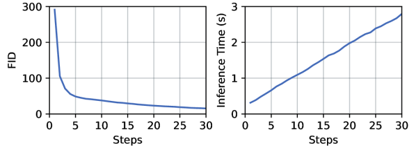
Figure 4. The FID scores (between images generated by our method and the complete generation process) and inference time of OLSS.

When a scheduler is applied to a diffusion model, there is a trade-off between efficiency and quality. Fewer steps can reduce the inference time but usually results in lower image quality. With the same settings as above, we apply OLSS to Stable Diffusion and calculate the FID scores with varying numbers of steps. We run the program on an NVIDIA A100 GPU and record the average time of generating an image. The results are plotted in Figure 4. As the number of steps increases, the FID score decreases rapidly at the beginning and gradually converges. The inference time increases almost linearly with the number of steps. Setting the number of steps to $5$, OLSS is able to generate an image within only one second, while still achieving satisfactory quality.

4.3. Visualization

To intuitively see how diffusion models generate images with different schedulers, we select $32$ examples randomly generated by Stable Diffusion in the above experiments. We catch the generation path $\{\boldsymbol{x}_{t(0)},\boldsymbol{x}_{t(1)},\dots,\boldsymbol{x}_{t(n)}\}$ and then embed these latent variables into a 2D plane using Principal Component Analysis (PCA). The embedded generation paths of three schedulers are shown in Figure 5. Starting from the same Gaussian noise $\boldsymbol{x}_{t(0)}$, these generation processes finally reach different $\boldsymbol{x}_{t(n)}$. In the complete generation process, $\boldsymbol{x}_{i}$ is updated gradually along a curve. The three 10-step schedulers construct an approximate generation process. We can see that the errors in the beginning steps are accumulated in the subsequent steps, thus the errors at the final steps become larger than those at the beginning. The generation path of OLSS is the closest one to the complete generation process, and the generation path of DPM-Solver++ is the second closest.

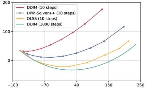
Figure 5. The generation path $\{\boldsymbol{x}_{t(0)},\boldsymbol{x}_{t(1)},\dots,\boldsymbol{x}_{t(n)}\}$ of three schedulers. We embed the latent variables to 2D using PCA to see the generation process intuitively.

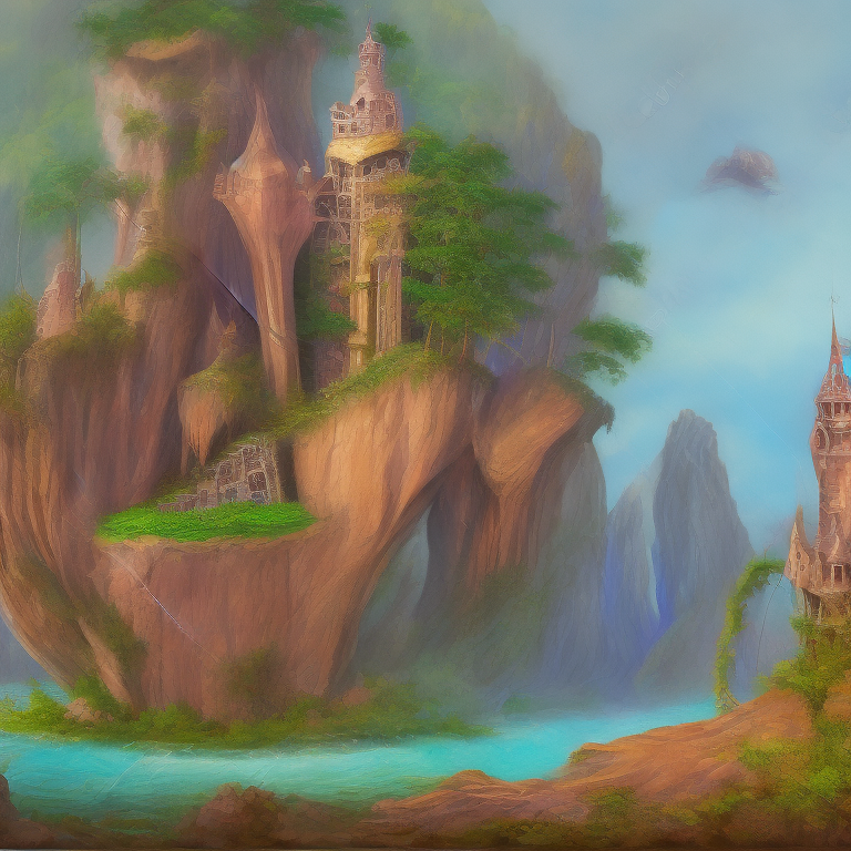
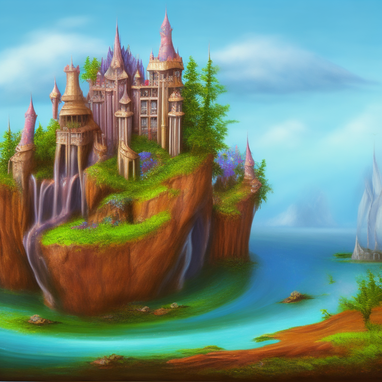
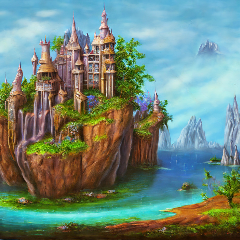
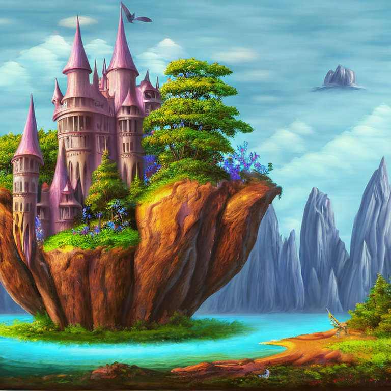
DDIM, 5 steps	DPM-Solver++, 5 steps	OLSS, 5 steps	DDIM, 1000 steps
(a) Prompt: “Fantasy magic castle on floating island. A very beautiful art painting.”
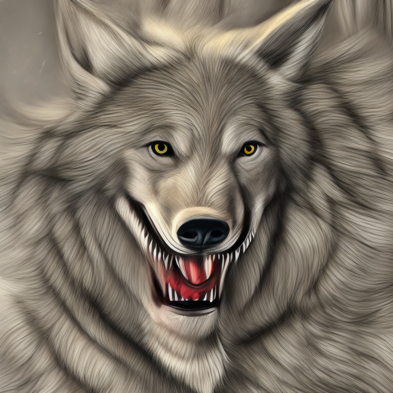
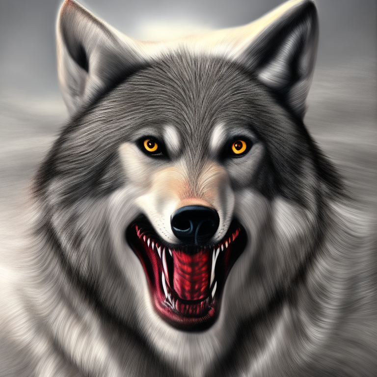
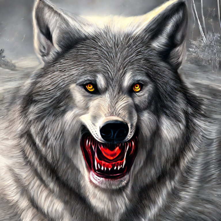
DDIM, 5 steps	DPM-Solver++, 5 steps	OLSS, 5 steps	DDIM, 1000 steps
(b) Prompt: “The leader of the wolves bared its ferocious fangs. High-resolution digital painting.”
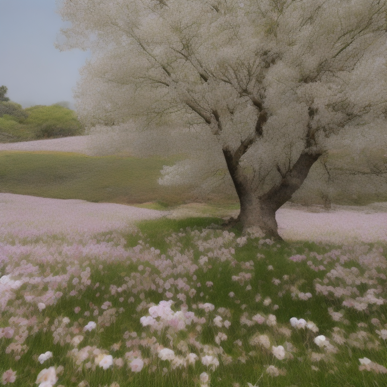
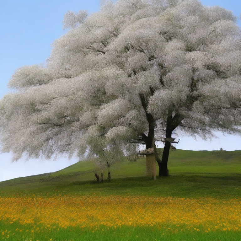
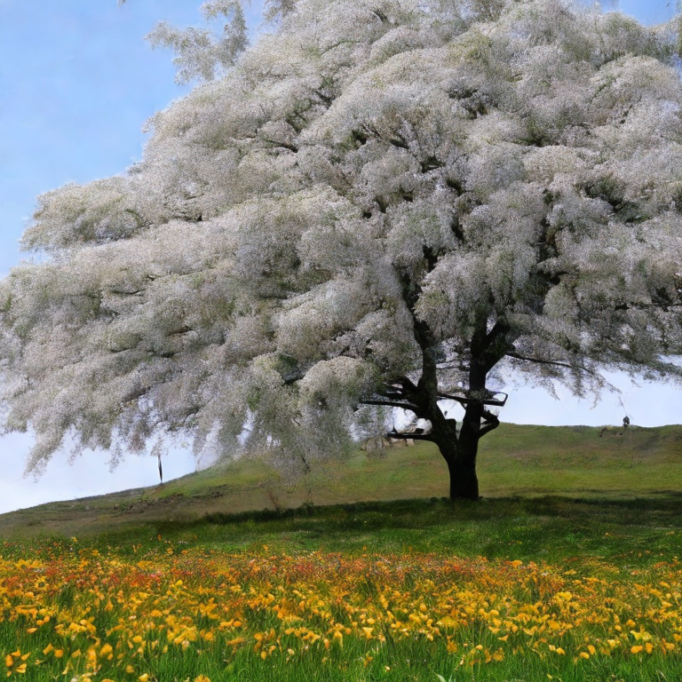
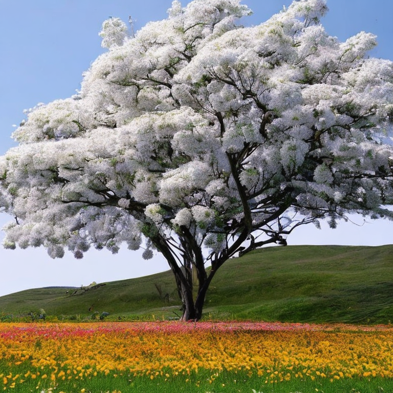
DDIM, 5 steps	DPM-Solver++, 5 steps	OLSS, 5 steps	DDIM, 1000 steps
(c) Prompt: “On the grassland, there is a towering tree with white flowers in full bloom, and under the tree are colorful flowers.”
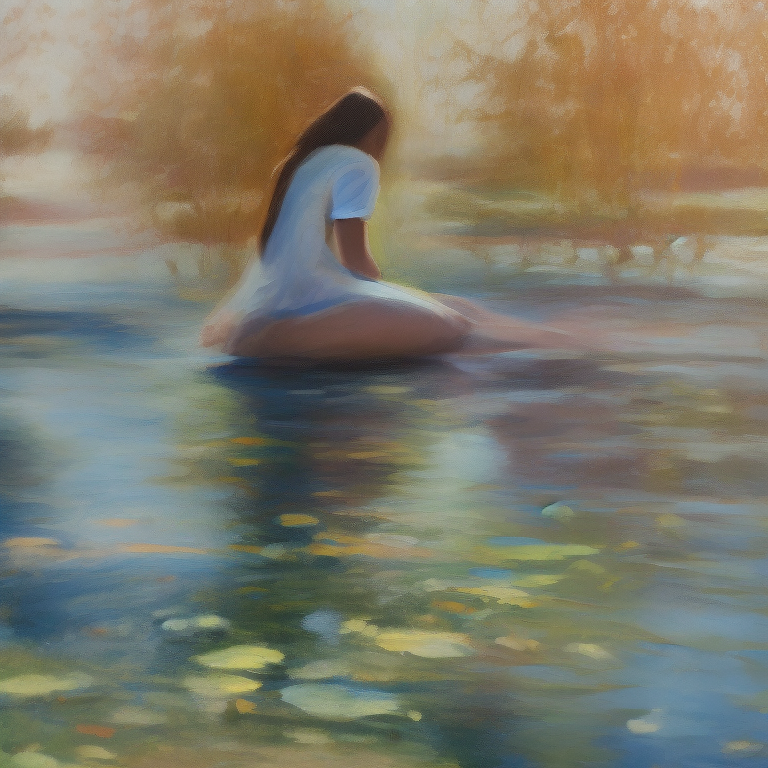
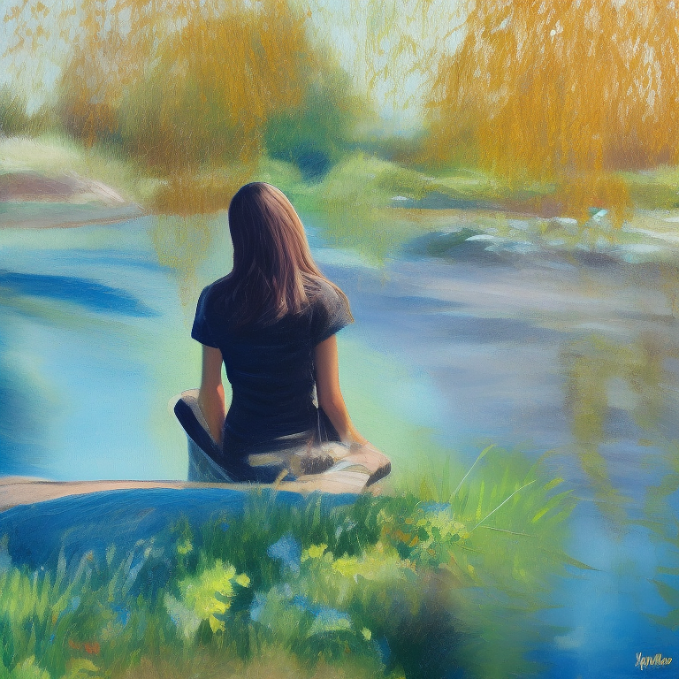
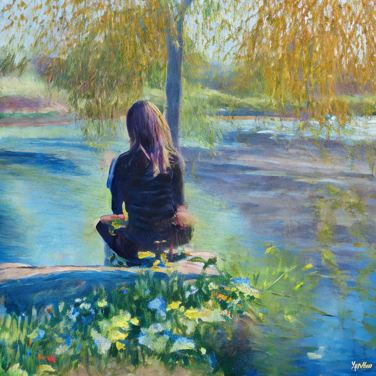
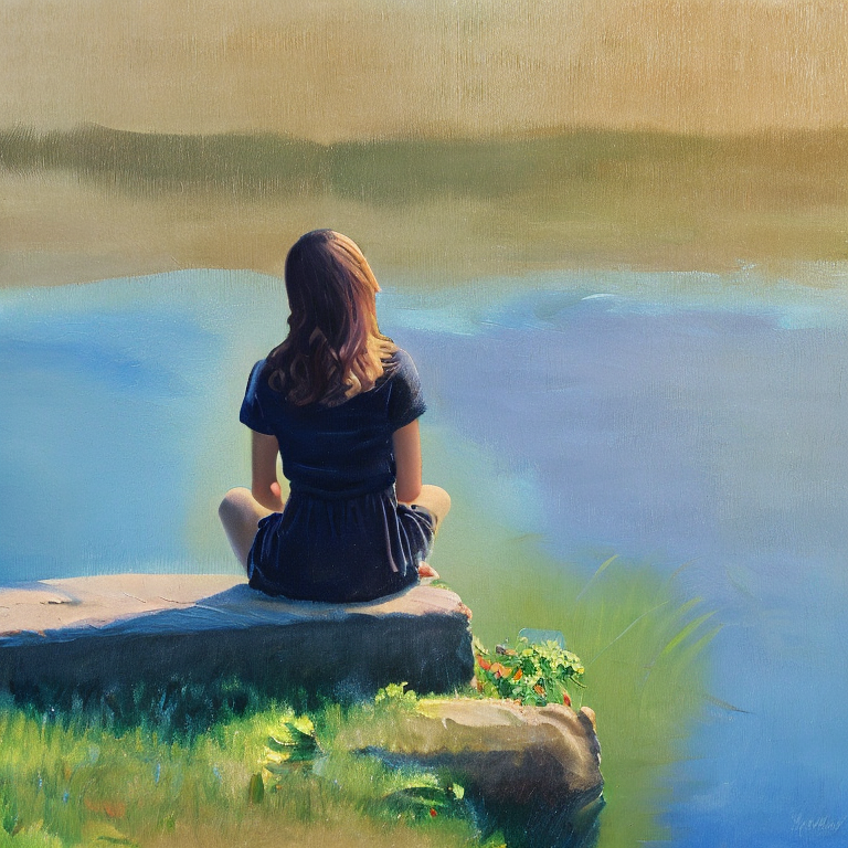
DDIM, 5 steps	DPM-Solver++, 5 steps	OLSS, 5 steps	DDIM, 1000 steps
(d) Prompt: “The girl sitting by the river looks at the other side of the river and thinks about life. Oil painting.”

Figure 6. Some examples generated by Stable Diffusion 2 with different schedulers and steps.

4.4. Case Study

In Figure 6, we present examples of images generated using Stable Diffusion 2 with DDIM, DPM-Solver++, and OLSS. Benefiting from the excellent generation ability of Stable Diffusion 2, we can generate exquisite artistic images. With only 5 steps, DDIM may make destructive changes to images. For instance, the castle in the first example looks smoggy. DPM-Solver++ tends to sharpen the entity at the expense of fuzzing details up. Only OLSS can clearly preserve the texture in the generated images (see the fur of the wolf in the second example and the flowers in the third example). In the fourth example, we observe that sometimes both DPM-Solver++ and OLSS generate images in a different style, where OLSS tends to generate more detail. Despite being generated with significantly fewer steps than 1000-step DDIM, the images generated by OLSS still look satisfactory. Hence, OLSS greatly improves the quality of generated images within only a few steps.

5. Conclusion and Future Work

In this paper, we investigate the schedulers in diffusion models. Specifically, we propose a new scheduler (OLSS) that is able to generate high-quality images within a very small number of steps. OLSS is a simple yet effective method that utilizes linear models to determine the coefficients in the iterative formula, instead of using mathematical theories. Leveraging the path optimization algorithm, OLSS can construct a faster process as an approximation of the complete generation process. The experimental results demonstrate that the quality of images generated by OLSS is higher than the existing schedulers with the same number of steps. In future work, we will continue investigating the generation process and explore improving the generative quality based on the modification in the latent space.

References

- (1)
- Björck (1990) Åke Björck. 1990. Least squares methods. Handbook of numerical analysis 1 (1990), 465–652.
- Butcher (2000) John C Butcher. 2000. Numerical methods for ordinary differential equations in the 20th century. J. Comput. Appl. Math. 125, 1-2 (2000), 1–29.
- Dhariwal and Nichol (2021) Prafulla Dhariwal and Alexander Nichol. 2021. Diffusion models beat gans on image synthesis. Advances in Neural Information Processing Systems 34 (2021), 8780–8794.
- Esser et al. (2023) Patrick Esser, Johnathan Chiu, Parmida Atighehchian, Jonathan Granskog, and Anastasis Germanidis. 2023. Structure and content-guided video synthesis with diffusion models. arXiv preprint arXiv:2302.03011 (2023).
- Feng et al. (2023) Zhida Feng, Zhenyu Zhang, Xintong Yu, Yewei Fang, Lanxin Li, Xuyi Chen, Yuxiang Lu, Jiaxiang Liu, Weichong Yin, Shikun Feng, et al. 2023. ERNIE-ViLG 2.0: Improving text-to-image diffusion model with knowledge-enhanced mixture-of-denoising-experts. In Proceedings of the IEEE/CVF Conference on Computer Vision and Pattern Recognition. 10135–10145.
- Goodfellow et al. (2020) Ian Goodfellow, Jean Pouget-Abadie, Mehdi Mirza, Bing Xu, David Warde-Farley, Sherjil Ozair, Aaron Courville, and Yoshua Bengio. 2020. Generative adversarial networks. Commun. ACM 63, 11 (2020), 139–144.
- Gu et al. (2022) Jiaxi Gu, Xiaojun Meng, Guansong Lu, Lu Hou, Niu Minzhe, Xiaodan Liang, Lewei Yao, Runhui Huang, Wei Zhang, Xin Jiang, et al. 2022. Wukong: A 100 million large-scale chinese cross-modal pre-training benchmark. Advances in Neural Information Processing Systems 35 (2022), 26418–26431.
- Heusel et al. (2017) Martin Heusel, Hubert Ramsauer, Thomas Unterthiner, Bernhard Nessler, and Sepp Hochreiter. 2017. Gans trained by a two time-scale update rule converge to a local nash equilibrium. Advances in neural information processing systems 30 (2017).
- Ho et al. (2020) Jonathan Ho, Ajay Jain, and Pieter Abbeel. 2020. Denoising diffusion probabilistic models. Advances in Neural Information Processing Systems 33 (2020), 6840–6851.
- Ho and Salimans (2021) Jonathan Ho and Tim Salimans. 2021. Classifier-Free Diffusion Guidance. In NeurIPS 2021 Workshop on Deep Generative Models and Downstream Applications.
- Huang et al. (2017) Xun Huang, Yixuan Li, Omid Poursaeed, John Hopcroft, and Serge Belongie. 2017. Stacked generative adversarial networks. In Proceedings of the IEEE conference on computer vision and pattern recognition. 5077–5086.
- Karras et al. (2017) Tero Karras, Timo Aila, Samuli Laine, and Jaakko Lehtinen. 2017. Progressive growing of gans for improved quality, stability, and variation. arXiv preprint arXiv:1710.10196 (2017).
- Karras et al. (2022) Tero Karras, Miika Aittala, Timo Aila, and Samuli Laine. 2022. Elucidating the design space of diffusion-based generative models. Advances in Neural Information Processing Systems 35 (2022), 26565–26577.
- Kerr et al. (2009) Andrew Kerr, Dan Campbell, and Mark Richards. 2009. QR decomposition on GPUs. In Proceedings of 2nd Workshop on General Purpose Processing on Graphics Processing Units. 71–78.
- Kingma and Welling (2013) Diederik P Kingma and Max Welling. 2013. Auto-Encoding Variational Bayes. In International Conference on Learning Representations.
- Liu et al. (2022) Jinglin Liu, Chengxi Li, Yi Ren, Feiyang Chen, and Zhou Zhao. 2022. Diffsinger: Singing voice synthesis via shallow diffusion mechanism. In Proceedings of the AAAI conference on artificial intelligence, Vol. 36. 11020–11028.
- Liu et al. (2021) Luping Liu, Yi Ren, Zhijie Lin, and Zhou Zhao. 2021. Pseudo Numerical Methods for Diffusion Models on Manifolds. In International Conference on Learning Representations.
- Lu et al. (2022a) Cheng Lu, Yuhao Zhou, Fan Bao, Jianfei Chen, Chongxuan Li, and Jun Zhu. 2022a. Dpm-solver: A fast ode solver for diffusion probabilistic model sampling in around 10 steps. Advances in Neural Information Processing Systems 35 (2022), 5775–5787.
- Lu et al. (2022b) Cheng Lu, Yuhao Zhou, Fan Bao, Jianfei Chen, Chongxuan Li, and Jun Zhu. 2022b. Dpm-solver++: Fast solver for guided sampling of diffusion probabilistic models. arXiv preprint arXiv:2211.01095 (2022).
- Nichol and Dhariwal (2021) Alexander Quinn Nichol and Prafulla Dhariwal. 2021. Improved denoising diffusion probabilistic models. In International Conference on Machine Learning. PMLR, 8162–8171.
- Odena et al. (2017) Augustus Odena, Christopher Olah, and Jonathon Shlens. 2017. Conditional image synthesis with auxiliary classifier gans. In International conference on machine learning. PMLR, 2642–2651.
- Radford et al. (2021) Alec Radford, Jong Wook Kim, Chris Hallacy, Aditya Ramesh, Gabriel Goh, Sandhini Agarwal, Girish Sastry, Amanda Askell, Pamela Mishkin, Jack Clark, et al. 2021. Learning transferable visual models from natural language supervision. In International conference on machine learning. PMLR, 8748–8763.
- Ramesh et al. (2022) Aditya Ramesh, Prafulla Dhariwal, Alex Nichol, Casey Chu, and Mark Chen. 2022. Hierarchical text-conditional image generation with clip latents. arXiv preprint arXiv:2204.06125 (2022).
- Reed et al. (2016) Scott Reed, Zeynep Akata, Xinchen Yan, Lajanugen Logeswaran, Bernt Schiele, and Honglak Lee. 2016. Generative adversarial text to image synthesis. In International conference on machine learning. PMLR, 1060–1069.
- Regalia (1993) Phillip A Regalia. 1993. Numerical stability properties of a QR-based fast least squares algorithm. IEEE Transactions on Signal Processing 41, 6 (1993), 2096–2109.
- Rombach et al. (2022) Robin Rombach, Andreas Blattmann, Dominik Lorenz, Patrick Esser, and Björn Ommer. 2022. High-resolution image synthesis with latent diffusion models. In Proceedings of the IEEE/CVF Conference on Computer Vision and Pattern Recognition. 10684–10695.
- Ronneberger et al. (2015) Olaf Ronneberger, Philipp Fischer, and Thomas Brox. 2015. U-net: Convolutional networks for biomedical image segmentation. In Medical Image Computing and Computer-Assisted Intervention–MICCAI 2015: 18th International Conference, Munich, Germany, October 5-9, 2015, Proceedings, Part III 18. Springer, 234–241.
- Saharia et al. (2022a) Chitwan Saharia, William Chan, Saurabh Saxena, Lala Li, Jay Whang, Emily L Denton, Kamyar Ghasemipour, Raphael Gontijo Lopes, Burcu Karagol Ayan, Tim Salimans, et al. 2022a. Photorealistic text-to-image diffusion models with deep language understanding. Advances in Neural Information Processing Systems 35 (2022), 36479–36494.
- Saharia et al. (2022b) Chitwan Saharia, Jonathan Ho, William Chan, Tim Salimans, David J Fleet, and Mohammad Norouzi. 2022b. Image super-resolution via iterative refinement. IEEE Transactions on Pattern Analysis and Machine Intelligence (2022).
- Salimans et al. (2016) Tim Salimans, Ian Goodfellow, Wojciech Zaremba, Vicki Cheung, Alec Radford, and Xi Chen. 2016. Improved techniques for training gans. Advances in neural information processing systems 29 (2016).
- Salimans and Ho (2021) Tim Salimans and Jonathan Ho. 2021. Progressive Distillation for Fast Sampling of Diffusion Models. In International Conference on Learning Representations.
- Schuhmann et al. (2022) Christoph Schuhmann, Romain Beaumont, Richard Vencu, Cade Gordon, Ross Wightman, Mehdi Cherti, Theo Coombes, Aarush Katta, Clayton Mullis, Mitchell Wortsman, et al. 2022. Laion-5b: An open large-scale dataset for training next generation image-text models. Advances in Neural Information Processing Systems 35 (2022), 25278–25294.
- Sohl-Dickstein et al. (2015) Jascha Sohl-Dickstein, Eric Weiss, Niru Maheswaranathan, and Surya Ganguli. 2015. Deep unsupervised learning using nonequilibrium thermodynamics. In International Conference on Machine Learning. PMLR, 2256–2265.
- Song et al. (2020) Jiaming Song, Chenlin Meng, and Stefano Ermon. 2020. Denoising Diffusion Implicit Models. In International Conference on Learning Representations.
- Song and Ermon (2019) Yang Song and Stefano Ermon. 2019. Generative modeling by estimating gradients of the data distribution. Advances in neural information processing systems 32 (2019).
- Szegedy et al. (2016) Christian Szegedy, Vincent Vanhoucke, Sergey Ioffe, Jon Shlens, and Zbigniew Wojna. 2016. Rethinking the inception architecture for computer vision. In Proceedings of the IEEE conference on computer vision and pattern recognition. 2818–2826.
- Vaswani et al. (2017) Ashish Vaswani, Noam Shazeer, Niki Parmar, Jakob Uszkoreit, Llion Jones, Aidan N Gomez, Łukasz Kaiser, and Illia Polosukhin. 2017. Attention is all you need. Advances in neural information processing systems 30 (2017).
- von Platen et al. (2022) Patrick von Platen, Suraj Patil, Anton Lozhkov, Pedro Cuenca, Nathan Lambert, Kashif Rasul, Mishig Davaadorj, and Thomas Wolf. 2022. Diffusers: State-of-the-art diffusion models. https://github.com/huggingface/diffusers.
- Watson et al. (2022) Daniel Watson, William Chan, Jonathan Ho, and Mohammad Norouzi. 2022. Learning fast samplers for diffusion models by differentiating through sample quality. In International Conference on Learning Representations.
- Yang et al. (2022) Ling Yang, Zhilong Zhang, Yang Song, Shenda Hong, Runsheng Xu, Yue Zhao, Yingxia Shao, Wentao Zhang, Bin Cui, and Ming-Hsuan Yang. 2022. Diffusion models: A comprehensive survey of methods and applications. arXiv preprint arXiv:2209.00796 (2022).
- Yu et al. (2015) Fisher Yu, Ari Seff, Yinda Zhang, Shuran Song, Thomas Funkhouser, and Jianxiong Xiao. 2015. Lsun: Construction of a large-scale image dataset using deep learning with humans in the loop. arXiv preprint arXiv:1506.03365 (2015).
- Zhang and Chen (2022) Qinsheng Zhang and Yongxin Chen. 2022. Fast Sampling of Diffusion Models with Exponential Integrator. In The Eleventh International Conference on Learning Representations.