Robust 3D-aware Object Classification via Discriminative Render-and-Compare

Abstract

In real-world applications, it is essential to jointly estimate the 3D object pose and class label of objects, i.e., to perform 3D-aware classification. While current approaches for either image classification or pose estimation can be extended to 3D-aware classification, we observe that they are inherently limited: 1) Their performance is much lower compared to the respective single-task models, and 2) they are not robust in out-of-distribution (OOD) scenarios. Our main contribution is a novel architecture for 3D-aware classification, termed RCNet, which builds upon a recent work[25] and performs comparably to single-task models while being highly robust. In RCNet, an object category is represented as a 3D cuboid mesh composed of feature vectors at each mesh vertex. Using differentiable rendering, we estimate the 3D object pose by minimizing the reconstruction error between the mesh and the feature representation of the target image. Object classification is then performed by comparing the reconstruction losses across object categories. Notably, the neural texture of the mesh is trained in a discriminative manner to enhance the classification performance while also avoiding local optima in the reconstruction loss. Furthermore, we show how RCNet and feed-forward neural networks can be combined to scale the render-and-compare approach to larger numbers of categories. Our experiments on PASCAL3D+, occluded-PASCAL3D+, and OOD-CV show that RCNet outperforms all baselines at 3D-aware classification by a wide margin in terms of performance and robustness.

1 Introduction

(a) Input image

(b) Feed-forward model

(c) Render-and-Compare

(d) RCNet

Figure 1: 3D-aware classification of a partially occluded car (a). Neither a feed-forward neural network (b) nor a render-and-compare approach (c) produce satisfying results as they only predict one task correctly but fail at the other. Our RCNet model (d) handles both tasks robustly, by following a render-and-compare approach building on a 3D-aware object representation with a discriminatively trained neural texture. For each plot (b-d), i shows a CAD mesh of the predicted category in the predicted 3D-pose, ii shows the predicted elevation angle (azimuth and in-plane rotation are not shown) and iii illustrates the classification prediction.

3D pose estimation and object classification are challenging but important tasks in computer vision. In real-world applications such as autonomous driving or robotics, it is crucial to solve both tasks jointly. Traditionally, these tasks were addressed with very different approaches. Object classification models typically apply a variant of feed-forward neural networks, such as Convolutional Neural Networks (CNNs) [15, 21, 7] or Transformers [4, 16]. In contrast, 3D pose estimation methods adopt a render-and-compare approach [25], where a given 3D object representation is fitted to an input image through inverse rendering. In this work, we study the task of 3D-aware object classification, i.e., jointly estimating the 3D object pose and class label. At first glance, one might be tempted to approach this novel task by extending either of the current approaches to object classification or pose estimation.

For example by extending CNNs with an additional pose estimation head or by following a render-and-compare approach and then comparing the final reconstruction results of different categories to obtain a class prediction. However, our experiments show that neither of these approaches lead to satisfying results. While feed-forward CNNs often serve as a baseline for 3D pose estimation [32, 25], they do not perform well enough, particularly in out-of-distribution scenarios (OOD) where objects are occluded or seen in an unusual pose [31]. Moreover, the predictions of the different CNN heads are often not consistent [30]. In contrast, render-and-compare approaches can estimate the 3D object pose accurately [10] and have been shown to be robust in OOD scenarios [25]. These methods learn 3D generative models of neural network features and perform pose estimation by reconstructing a target image in feature space. However, we observe that these approaches do not perform well at object classification because they require a separate feature extractor per object class. Hence, their features are not trained to discriminate between classes. Moreover, render-and-compare approaches are computationally much more expensive than feed-forward CNNs, because the pose optimization needs to be performed for all target object classes.

In this paper, we introduce Render-and-Compare-Net (RCNet), a novel architecture that performs classification and pose estimation in a unified manner while being highly robust in OOD scenarios. Our model significantly extends recent works for pose estimation [25, 10] that represent objects as meshes with a neural texture, i.e., neural feature vector at each mesh vertex. Our first contribution is that we train the neural texture to be discriminative and hence to enable object classification. In particular, the features are trained using contrastive learning to be distinct between different classes while also being invariant to instance-specific details within an object category (such as shape and color variations). To capture the remaining variation in the neural texture within an object category, we train a generative model of the feature activations at every vertex of the mesh representation. Importantly, our model implements a factorized model where feature vectors are conditionally independent given the object class and pose, which enables rapid inference and robustness. During inference, RCNet first extracts the feature map of a target image using a CNN and subsequently optimizes the 3D pose of the mesh to best reconstruct the target feature map using gradient-based optimization. Finally, we perform object classification by comparing the reconstruction losses across all categories, leading to state-of-the-art 3D-aware classification results. Additionally, we leverage the output of feed-forward CNNs as proposals for RCNet to reach a sweet spot at which the combined model uses the fast-to-compute CNN output when the test data is easy to classify while falling back to the more expensive but reliable RCNet branch in difficult OOD cases.

We evaluate RCNet on the PASCAL3D+ [28], the occluded-PASCAL3D+ [25], and OOD-CV [31], which was explicitly designed to evaluate out-of-distribution generalization in computer vision models. Our experiments show that RCNet outperforms all baselines at 3D-aware classification by a wide margin. Our contributions are:

1. We introduce RCNet, a 3D-aware neural network architecture that follows an inverse rendering approach and leverages discriminatively trained neural textures to perform 3D-aware classification.

2. We demonstrate that feed-forward neural networks and render-and-compare approaches can be combined to reach a sweet spot that trades off fast but unreliable predictions with robust but computationally expensive reasoning to achieve state-of-the-art performance.

3. We observe that RCNet is exceptionally robust in out-of-distribution scenarios.

2 Related Work

Category-level 3D pose estimation. Multiple approaches have been proposed for category-level 3D pose estimation. The most classical approach is to formulate object pose estimation as a classification problem [23, 18]. Another approach is a two-step keypoint-based method [32] that extracts semantic keypoints first, then solves a Perspective-n-Point problem for optimal 3D pose. The most recent works adopt a render-and-compare approach [25] that moves from pixel-level image synthesis to feature-level representation synthesis. In render-and-compare, 3D pose is predicted by minimizing a reconstruction error between a mesh-projected feature map and an extracted feature map. Our method adopts the render-and-compare approach as a basis, making it capable of robust object classification.

Robust Image Classification. Image Classification is a significant task in computer vision. Multiple influential architectures include Resnet [7], Transformer [24], and recent Swin-Transformer [16] have been designed for this task. However, these models are not robust enough to handle partially occluded images or out-of-distribution data. Efforts that have been made to close the gap can be mainly categorized into two types: data augmentation and architectural design. Data augmentation includes using learned augmentation policy [3], and data mixture [8]. Architectural changes propose robust pipelines. For instance, [12] proposes an analysis-by-synthesis approach for a generative model to handle occlusions. In addition, new benchmarks like ImageNetA subset [9] and OOD-CV [31] that test classification robustness are also designed. These benchmarks have been proven to drop the performance of standard models by a large margin, and our model is evaluated on one of these benchmarks to classify images robustly.

Feature-level render-and-compare. Render-and-compare methods optimize the predicted pose by reducing the reconstruction error between 3D-objects projected feature representations and the extracted feature representations. It can be seen as an approximate analysis-by-synthesis [6] approach, which, unlike discriminative methods, has been proven to be robust against out-of-distribution data. It has been proven useful, especially against partially occluded data, in object classification [13] and 3D pose estimation [25, 11]. Our method extends this analysis-by-synthesis approach to achieve robust object classification and 3D pose estimation.

3 Method

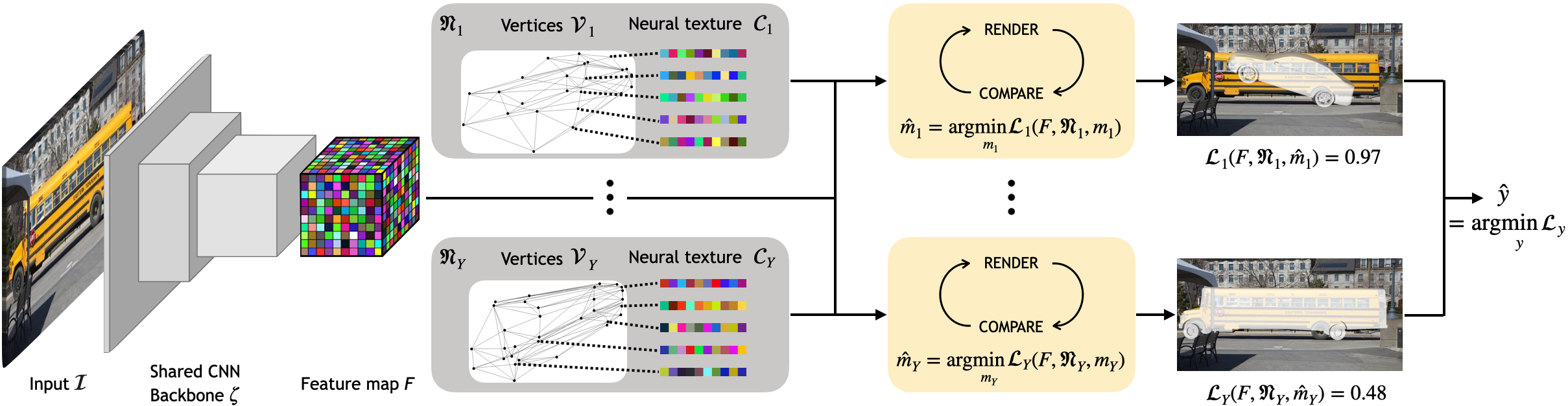
Figure 2: An overview of our RCNet pipeline. For each image, the network $\zeta$ extracts a feature map $F$. Meanwhile, we render feature maps $F^{\prime}_{y}$ using our class-specific trained Neural Mesh Models $\mathfrak{N}_{y}$ and optimize the pose $m_{y}$ using a feature-level render-and-compare approach. Lastly, we compare the different losses $\mathcal{L}_{y}(F,\mathfrak{N},m)$ to infer the object category $\hat{y}$. We visualize the pose prediction for two different object categories. Note that for illustration purposes, we visualize a projection of a CAD model but our RCNet is using cuboid meshes with much lower detailed geometry and we omit the background model $\mathcal{B}$ and the subscript $\mathcal{L}_{NLL}$ in the loss notation.

In this section, we introduce our notations (Sec. 3.1); we review the render-and-compare approach for pose estimation in Section 3.2. Next, the architecture of our RCNet model and its training and inference processes are introduced in Section 3.3. Finally, we discuss how RCNet can be scaled efficiently with feed-forward models in Section 3.4.

3.1 Notation

We denote a feature representation of an input image $\mathcal{I}$ as $\zeta(I)=F^{l}\in\mathbb{R}^{H\times W\times c}$. Where $l$ is the output of layer $l$ of a deep CNN $\zeta$, with $c$ being the number of channels in layer $l$. $f^{l}_{i}\in\mathbb{R}^{c}$ is a feature vector in $F^{l}$ at position $i$ on the 2D lattice $\mathcal{P}$ of the feature map. In the remainder of this section, we omit the superscript $l$ for notation simplicity because this is fixed a-priori in our model.

3.2 Render-And-Compare for Pose Estimation

Our work builds on and significantly extends Neural Mesh Models (NMMs) [25], which are 3D extensions of Compositional Generative Networks (GCN) [12]. For each object category $y$, NMMs defines a neural mesh $\mathfrak{N}_{y}$ as $\{\mathcal{V},\mathcal{C}\}$, where $\mathcal{V}=\{V_{r}\in\mathbb{R}^{3}\}_{r=1}^{R}$ is the set of vertices of the mesh and $\mathcal{C}=\{C_{r}\in\mathbb{R}^{c}\}_{r=1}^{R}$ is the set of learnable features. Moreover, $c$ is the number of channels in layer $l$, and $R$ is the number of vertices in the mesh. Each mesh is a cuboid (referred as SingleCuboid in [25]) with a fixed scale determined by the average size of all sub-category meshes in the dataset. We refer to the set of features on the mesh $\mathcal{C}$ as neural texture, the terminology of computer graphics literature. We capture the variability in the feature activations in the data with a statistical distribution that defines the likelihood of a target real-valued feature map $F\in\mathbb{R}^{H\times W\times D}$ using the neural mesh $\mathfrak{N}_{y}$ as

$$p(F\!\mid\!\mathfrak{N}_{y},m,\mathcal{B})=\prod_{i\in\mathcal{FG}}\!p(f_{i}\!\mid\!\mathfrak{N}_{y},m)\prod_{i^{\prime}\in\mathcal{BG}}\!p(f_{i^{\prime}}\!\mid\!\mathcal{B}),$$ (1)

where $m$ is the camera parameters for projecting the neural mesh $\mathfrak{N}_{y}$ into the image. The foreground $\mathcal{FG}$ is the set of all positions on the 2D lattice $\mathcal{P}$ of the feature map $F$ that are covered by the rendered neural mesh and as opposed to the background $\mathcal{BG}=\mathcal{P}\backslash\{\mathcal{FG}\}$. Both foreground feature likelihood and background feature likelihood are defined as Gaussian distributions. The foreground has $p(f_{i}\mid\mathfrak{N}_{y},m)=\mathcal{N}(f_{i}\mid C_{r},\sigma_{r}^{2}I)$, and the background has $p(f_{i^{\prime}}\mid\mathcal{B})=\mathcal{N}(f_{i^{\prime}}\mid b,\sigma^{2}I)$ with $\mathcal{B}=\{b,\sigma\}$. $C_{r}$ is the learned neural texture for the vertice, and $b$ is the mean of the learned noise neural texture in the background.

Maximum likelihood estimation (MLE) is adopted to train the feature extractor and the model parameters $\{\mathfrak{N},B\}$. Then at inference time, we render and compare for the pose $m$ by minimizing the negative log-likelihood of the model w.r.t. the pose $m$ using gradient descent.

$$\mathcal{L}_{\text{NLL}}(F,\mathfrak{N}_{y},m,\mathcal{B})=-\ln p(F\mid\mathfrak{N}_{y},m,\mathcal{B})$$

$$= -\sum_{i\in\mathcal{FG}}\left(\ln\left(\frac{1}{\sigma_{r}\sqrt{2\pi}}\right)-\frac{1}{2\sigma_{r}^{2}}\lVert f_{i}-C_{r}\rVert^{2}\right)$$

$$-\sum_{i^{\prime}\in\mathcal{BG}}\left(\ln\left(\frac{1}{\sigma\sqrt{2\pi}}\right)-\frac{1}{2\sigma^{2}}\lVert f_{i^{\prime}}-b\rVert^{2}\right).$$ (2)

Assuming unit variance [25] with $\sigma_{r}=\sigma=1$, the loss function 2 reduces to the sum of the mean squared error (MSE) from foreground neural texture features and background noise neural texture features to the target feature map.

$$\mathcal{L}_{\text{NLL}}(F,\mathfrak{N}_{y},m,\mathcal{B})= \frac{1}{2}\sum_{i\in\mathcal{FG}}\lVert f_{i}-C_{r}\rVert^{2}$$

$$+\frac{1}{2}\sum_{i^{\prime}\in\mathcal{BG}}\lVert f_{i}-b\rVert^{2}+\textit{const.}$$ (3)

Previous works adopted this general framework for category-level 3D pose estimation [25, 26]. In this work, we demonstrate that such a feature-level render-and-compare approach can be generalized beyond pose estimation to include object classification, by training the neural texture to discriminate among object classes. Then we show that such new models can handle 3D-aware object classification well.

3.3 RCNet for 3D-Aware Object Classification

Prior methods that follow a feature-level render-and-compare approach are limited to pose estimation tasks and therefore need to assume that the object class is known a-priori. Intuitively, these works can be extended to perform object classification by predicting the class label as the object model that can best reconstruct a target image:

$$\{\hat{y},\hat{m}_{\hat{y}}\}=\operatorname*{arg\,min}_{y,m}\mathcal{L}_{\text{NLL}}(F,\mathfrak{N}_{y},m,\mathcal{B}),$$ (4)

where $\{\hat{y},\hat{m}_{\hat{y}}\}$ are the object class and corresponding object pose with minimal negative-log-likelihood. However, this approach has several limitations: 1) The feature representations in all prior works cannot discriminate between classes. Hence, the likelihood is not a good indicator for class prediction (see experiments in Section 4). 2) It is important to note that all prior works on pose estimation have an independent backbone and mesh model for each category. The lack of a shared backbone makes it hard to define a discriminative loss for a classification task. 3) Optimizing Equation 4 requires running the render-and-compare process for all object classes, which is computationally expensive.

In the following, we introduce RCNet, a novel architecture that addresses these problems by introducing a shared backbone, a contrastive classification loss and a principled way of integrating feed-forward neural networks into the render-and-compare process to make 3D-aware classification with render-and-compare computationally efficient.

3.3.1 RCNet Architecture and Inference Process

In this work, we generalize feature-level render-and-compare approaches to object classification by learning neural textures that are invariant to variations in the object shape and appearance while at the same time being discriminative among different object categories. Figure 2 illustrates the architecture and inference process of our RCNet. An input image $\mathcal{I}$ is first processed by a CNN backbone $\zeta$ into a feature map $F$. A core difference to related work [25, 11] is that RCNet builds on a shared CNN backbone instead of separate backbones for different categories. The shared backbone enables us to integrate a discriminative loss into the learning process to encourage the neural textures of different object classes to be distinct (Section 3.3.2). Subsequently, by minimizing the negative-log-likelihood in Equation 3 through gradient-based optimization, we perform a render-and-compare optimization for every object category $\{\mathfrak{N}_{y}\}$ to obtain the optimal pose $\hat{m}_{y}$ for each object category. The object category $\hat{y}$ that achieves the highest likelihood will be the predicted class, hence performing 3D-aware classification in a unified manner (Eq. 4). We explain the learning procedure in the following and discuss how it can be scaled efficiently in Section 3.4.

3.3.2 Learning Discriminative Neural Textures

In order to enable 3D-aware classification via render-and-compare, the features extracted by the shared CNN backbone $\zeta$ need to fulfill three properties: 1) They need to be invariant to instance-specific details within a category. 2) They should avoid local optima in the loss landscape. 3) Comparing the minimal reconstruction losses of different object categories should enable object classification. To achieve the first two properties, we train the feature extractor $\zeta$ using contrastive learning to learn distributed features akin to the probabilistic generative model as defined in Equations 1-3. We adopt an image-specific contrastive loss as in [25]:

$$\mathcal{L}_{\text{con}}(F)=-\!\sum_{i\in\mathcal{FG}}\!\sum_{j\in\mathcal{FG}}\!\lVert\!f_{i}\!-\!f_{j}\!\rVert^{2}-\!\sum_{i\in\mathcal{FG}}\!\sum_{j\in\mathcal{BG}}\!\lVert\!f_{i}\!-\!f_{j}\!\rVert^{2},$$ (5)

which encourages the features at different positions on the object to be distinct from each other (first term), while also making the features on the object distinct from the features in the background (second term).

Moreover, we introduce a class-contrastive loss encouraging the neural textures among different meshes to be distinct from each other:

$$\mathcal{L}_{\text{class}}(\{C_{y}\})=-\sum_{y=1}^{Y}\sum_{\bar{y}=1\setminus\{y\}}^{Y}\lVert\mu(y)-\mu(\bar{y})\rVert^{2},$$ (6)

where $\mu(y)=\sum_{i=1}^{N}C_{i,y}/N$ is the mean of the neural texture $C_{y}$ of class $y$. Our full model is trained by optimizing the joint loss:

$$\mathcal{L}_{joint}=\mathcal{L}_{\text{con}}+\mathcal{L}_{\text{class}},$$ (7)

The joint loss $\mathcal{L}_{\text{joint}}$ is optimized in a contrastive learning framework, where we update the parameters of the feature extractor $\zeta$ and the neural textures $\mathcal{C}$ jointly.

MLE of neural textures. We train the parameters of the neural texture $\mathcal{C}$ through maximum likelihood estimation (MLE) by minimizing the negative log-likelihood of the feature representations over the whole training set (Equation 3). The correspondence between the feature vectors $f_{i}$ and vertices $r$ is computed using the annotated 3D pose. To reduce the computational cost of optimizing Equation 3, we update $\mathcal{C}$ in a moving average manner [1].

Dataset	(Occluded) PASCAL3D+					OOD-CV
Nuisance	L0	L1	L2	L3	Mean	Context	Pose	Shape	Texture	Weather	Mean
Resnet50	99.3	93.8	77.8	45.2	79.6	54.7	63.0	59.3	59.5	51.3	57.2
Swin-Transformer-T	99.4	93.6	77.5	46.2	79.7	58.2	66.6	63.9	61.6	54.6	60.8
NeMo	88.0	72.5	49.3	22.3	58.3	52.2	43.2	54.8	45.5	40.4	46.3
Ours	99.1	96.1	86.8	59.1	85.3	85.2	88.2	84.6	90.3	82.4	86.0
Ours+Scaling	99.4	96.2	87.0	59.2	85.5	85.1	88.1	84.1	88.5	82.7	85.4

Table 1: Classification accuracy results on (Occluded) PASCAL3D+ and OOD-CV dataset. Occlusion level L0 are unoccluded images from PASCAL3D+ dataset, and occlusion level L1, L2, L3 are from Occluded PASCAL3D+ dataset with occlusion ratios stated in 4.1.

Dataset		(Occluded) PASCAL3D+					OOD-CV
Nuisance		L0	L1	L2	L3	Mean	Context	Pose	Shape	Texture	Weather	Mean
$ACC_{\frac{\pi}{6}}\uparrow$	Resnet50	82.2	66.1	53.1	42.1	61.3	57.8	34.5	50.5	61.5	60.0	51.8
	Swin-Transformer-T	84.4	67.9	50.4	36.6	60.3	52.9	34.6	48.2	57.2	60.9	50.4
	NeMo	87.4	75.9	63.9	45.6	68.6	50.3	35.3	49.6	57.5	52.2	48.0
	Ours	86.1	74.8	59.2	37.3	64.4	54.3	38.0	53.5	60.5	57.3	51.9
	Ours+Scaling	89.8	78.1	62.6	39.0	67.9	55.4	36.7	53.1	60.0	57.0	51.4
$ACC_{\frac{\pi}{18}}\uparrow$	Resnet50	39.0	25.5	16.9	8.9	22.9	15.5	12.6	15.7	22.3	23.4	18.0
	Swin-Transformer-T	46.2	28.0	14.8	7.1	24.5	18.3	14.4	16.9	21.1	26.3	19.8
	NeMo	62.9	45.0	31.3	15.8	39.2	21.9	6.9	19.5	34.0	30.4	21.9
	Ours	61.6	42.8	27.0	11.6	35.8	23.6	10.4	22.7	37.5	35.5	25.5
	Ours+Scaling	65.1	45.0	28.7	12.5	38.4	23.5	9.8	22.3	37.9	34.5	24.8

Table 2: Pose Estimation results on (Occluded) PASCAL3D+, and OOD-CV dataset. Pose accuracy is evaluated for error under two thresholds: $\frac{\pi}{6}$ and $\frac{\pi}{18}$ separately. Noticeably, our RCNet is most robust on OOD-CV dataset for pose estimation on average.

3.4 Scaling Render-and-Compare Efficiently

RCNet model is highly robust and outperforms related works on various challenging dataset. However, one limitation of the inverse rendering approach to 3D-aware classification is that a naïve implementation requires running the render-and-compare optimization for every object class. This approach scales linearly with the number of target object classes. In contrast, feed-forward neural networks scale much more efficiently but are far less robust (see experiments in Section 4). A natural question arises that we want to address in this section: Can we integrate the fast inference of feed-forward neural networks with our robust render-and-compare approach to retain the best of both worlds? Hence, we seek a trade-off between a fast prediction and a more elaborate but robust render-and-compare process. Notably, such a combined approach loosely relates to feed-forward and feedback mechanisms for visual recognition in monkey and human vision [17, 14, 19].

In order to take advantage of the complementary strengths of feed-forward models and our RCNet, we first train a CNN with two output heads for predicting both the object class and the 3D object pose (see Section 4 for details on the training and architecture). For a given input image $I$, the CNN predicts the corresponding probability for the object class $p(y|\mathcal{I};\bf{w})$ and object pose $p(m|\mathcal{I};\bf{w})$ respectively, with $\bf{w}$ being the learned weights of the model. In the following, we describe a three-step process combining the CNN output with RCNet to reduce the overall computation time while improving its robustness in OOD scenarios.

Handle simple cases using CNN predictions ($S_{1}$).

We take advantage of the ability of deep neural networks to approximately estimate the confidence of their prediction, which has been observed in prior works [5, 13], and can be confirmed from our experimental results in Section 4.3. In particular, we observe that when the test data is similar to the training data, the feed-forward model is typically very confident, whereas in challenging OOD scenarios, the prediction confidence is reduced. We leverage this property and first process every test image $I$ with the CNN, and retain the class prediction $\hat{y}_{\text{cnn}}$ if the prediction confidence exceeds a threshold $p(y_{\text{cnn}}|I;\bf{w})>\tau_{1}$ with $\tau_{1}=0.95$ being experimentally defined. This enables us to perform a fast classification in simple cases, and we demonstrate the efficacy of this approach on various challenging datasets. However, we find the multi-headed CNN pose prediction to be less reliable than the class prediction (Section 4.3). Therefore, we apply it as initialization to speed up the convergence of the render-and-compare optimization of RCNet in these simple cases.

Verify CNN proposals with generative models in difficult cases ($S_{2}$).

To enhance the processing time of test data even in difficult cases, where the CNN output is unreliable, we use the combined CNN output of object class and pose predictions as initialization that is to be verified by the more demanding RCNet optimization in a ”top-down” manner. Notably, such a bottom-up and top-down processing was advocated in classical prior works for object segmentation [2, 22] or face reconstruction [20]. Specifically, we use the predicted top-3 classes and respective top-3 poses of the CNN and the rendering process in RCNet to compute their respective reconstruction losses. We start a complete render-and-compare optimization process from the CNN prediction that achieves the lowest reconstruction loss.

Full render-and-compare optimization when uncertain ($S_{3}$).

The final reconstruction error of RCNet can indicate if the render-and-compare optimization has converged to a good solution (Section 4). While the reconstruction error is a much more expensive form of feedback compared to the output of the feed-forward CNN, it is also a more reliable indicator of the pose prediction quality. We use it to estimate if the render-and-compare process that was initialized by the CNN output was successful by thresholding the reconstruction loss with $\tau_{2}=0.9$. Only for those test images that fall below this threshold, we run the computationally most expensive prediction by starting the inverse rendering process from several randomly initialized starting points and keep the best solution as described in Section 4.1.

In summary, we introduce a principled way of integrating the fast but not robust predictions of feed-forward CNNs with our RCNet model, reducing the overall computation time by 41% compared to a naïve implementation of RCNet. We note that this process is optional and only applies if a reduced computation time is desired.

4 Experiments

In this section, we first describe the experimental setup in Section 4.1. Subsequently, we study the performance of RCNet in IID and OOD scenarios in Section 4.2. Finally, scaling results are provided in Section 4.3.

4.1 Setup

Datasets. We evaluate RCNet on three datasets: PASCAL3D+ [29], Occluded PASCAL3D+[27], and Out-of-Distribution-CV (OOD-CV)[31]. PASCAL3D+ includes 12 object categories, and each object is annotated with 3D pose, object centroid, and object distance. The dataset provides a 3D mesh for each category. We split the dataset into a training set of 11045 images and a validation set with 10812 images, referred to as L0. Building on the PASCAL3D+ dataset, the occluded PASCAL3D+ dataset is a benchmark that evaluates robustness under different levels of occlusion. It simulates realistic occlusion by superimposing occluders on top of the objects with three different levels: L1: 20%-40%, L2: 40%-60%, L3:60%-80%. The OOD-CV dataset is a benchmark dataset that includes OOD examples of 10 object categories varying in terms of 5 nuisance factors: pose, shape, context, texture, and weather.

Implementation details. RCNet consists of a category-specific neural mesh and a shared feature extractor backbone. Each mesh contains approx. $1100$ vertices distributed uniformly on the cuboid. The shared feature extractor $\zeta$ is a Resnet50 model with two upsampling layers. The size of the feature map $F$ is $\frac{1}{8}$ of the input size. All images are cropped or padded to $640\times 800$. The feature extractor and neural textures of all object categories are trained collectively, taking around 20 hours on 8 RTX 2080Ti.

RCNet inference follows Section 3.3.1. We extract a feature map $F$ from an input image using our shared feature extractor, then apply render-and-compare to render each neural mesh into a feature map $F_{y}^{\prime}$. For initializing the pose estimation, we follow [25] and sample $144$ poses ($12$ azimuth angles, $4$ elevation angles, $3$ in-plane rotations) and choose the pose with the lowest reconstruction error as initialization. We minimize the reconstruction loss of each category (Equation 3) to estimate the object pose. The category achieving the minimal reconstruction loss is selected as the class prediction. Inference takes 0.8s on 8 RTX 2080Ti.

Dataset		(Occluded) PASCAL3D+					OOD-CV
Nuisance		L0	L1	L2	L3	Mean	Context	Pose	Shape	Texture	Weather	Mean
$ACC_{\frac{\pi}{6}}\uparrow$	Resnet50	81.8	62.9	42.8	20.6	52.7	31.2	12.7	24.6	32.0	25.8	23.9
	Swin-Transformer-T	83.9	64.9	41.9	19.5	53.2	29.5	14.5	24.6	30.6	28.8	24.8
	NeMo	82.4	62.1	39.1	13.3	50.0	36.3	22.0	35.4	34.0	31.5	31.0
	Ours	85.8	73.8	57.0	30.8	61.9	51.2	36.9	48.1	58.5	55.1	49.2
	Ours+Scaling	89.7	77.2	60.0	32.1	65.4	53.6	36.3	49.3	59.1	55.6	49.7
$ACC_{\frac{\pi}{18}}\uparrow$	Resnet50	45.6	27.6	14.9	5.1	23.7	6.0	2.8	4.7	6.5	7.4	5.4
	Swin-Transformer-T	46.1	22.7	12.9	4.2	21.9	7.2	3.3	6.3	6.2	8.2	6.2
	NeMo	60.1	38.9	21.1	5.2	31.9	17.8	4.9	14.2	22.8	20.3	15.3
	Ours	61.5	42.6	26.6	10.6	35.9	22.8	10.2	21.7	36.5	34.9	24.9
	Ours+Scaling	65.0	44.7	28.1	11.2	37.8	22.8	9.7	21.7	37.5	34.1	24.4

Table 3: 3D-aware Object Classification (i.e., simultaneously estimating the object class and its 3D pose) results on (Occluded) PASCAL3D+ and OOD-CV datasets. Our performance is significantly better than baselines with a large margin in all datasets.

Metric	$ACC_{\frac{\pi}{6}}\uparrow$					$ACC_{\frac{\pi}{18}}\uparrow$					Computation cost $\downarrow$ (in % of the reference)
Nuisance	L0	L1	L2	L3	Mean	L0	L1	L2	L3	Mean	L0	L1	L2	L3	Mean
Ours	85.8	73.8	57.0	30.8	61.9	61.5	42.6	26.6	10.6	35.9	100	100	100	100	100
Ours$+S_{1}$	85.6	73.8	57.0	30.8	61.8	61.3	42.4	26.3	10.4	35.7	25	72	93	99	72
Ours$+S_{1}\!+\!S_{2}$	87.6	70.1	51.3	25.8	59.4	63.8	41.2	23.9	9.0	35.0	8	24	31	33	24
Ours$+$Scaling	89.7	77.2	60.0	32.1	65.4	65.0	44.7	28.1	11.2	37.8	12	44	75	106	59

Table 4: Ablation of our model components at 3D-aware classification on the (Occluded) PASCAL3D+ dataset. Ours refers to RCNet described in 3.3. $S_{1}$ refers to the thresholding of simple cases for class predictions. $S_{2}$ refers to CNN proposals for classes and initialization of the generative model. Ours+Scaling (equivalent to Ours$+S_{1}\!+\!S_{2}+\!S_{3}$ with $S_{3}$ referring to the thresholding on reconstruction loss) refers to the full combination of RCNet and the feed-forward model as described in 3.4.

Evaluation. We evaluate the tasks classification, pose estimation, and 3D-aware classification. The 3D pose estimation involves predicting azimuth, elevation, and in-plane rotations of an object with respect to a camera. Following [32], the pose estimation error is calculated between the predicted rotation matrix $R_{pred}$ and the ground truth rotation matrix $R_{gt}$ as $\Delta\left(R_{pred},R_{gt}\right)=\frac{\left\|\log m\left(R_{pred}^{T}R_{gt}\right)\right\|_{F}}{\sqrt{2}}$. We use two common thresholds $\frac{\pi}{6}$ and $\frac{\pi}{18}$ to measure the prediction accuracy. We note that for a correct 3D-aware classification, the model must estimate both the class label and 3D object pose correctly.

Baselines. We compare our RCNet to three baselines. The first baseline is an extended Resnet50 model that has two classification heads. One head estimates pose estimation as a classification problem, and another head is used for regular object category classification. The second baseline is a Swin-Transformer-T [16] that has a similar setting as Resnet50, and the third baseline is NeMo [25], which is also a render-and-compare approach.

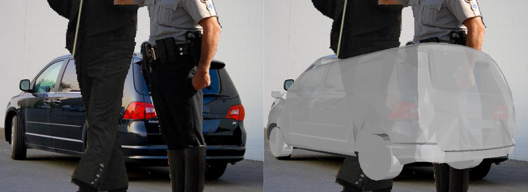
(a) L2 Occluded, Car

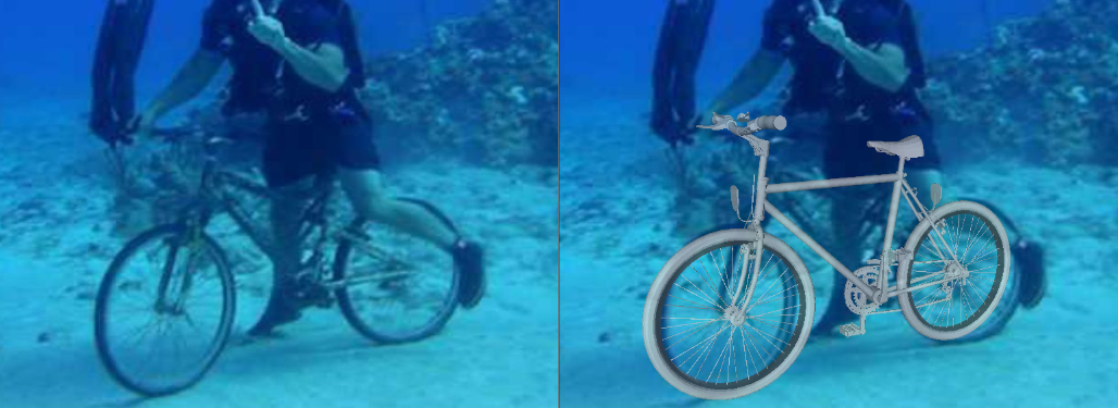
(b) Context OOD, Bicycle

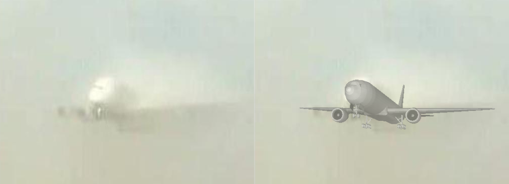
(c) Weather OOD, Aeroplane

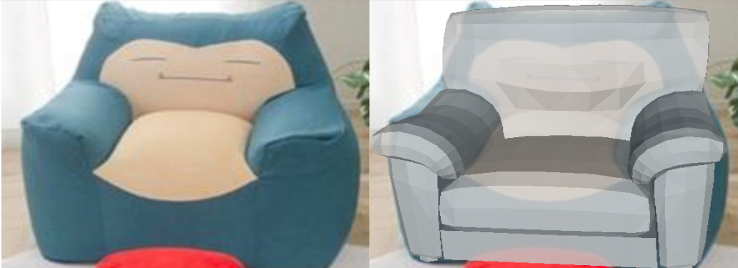
(d) Texture OOD, Sofa

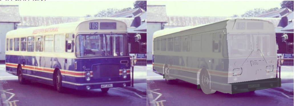
(e) Shape OOD, Bus

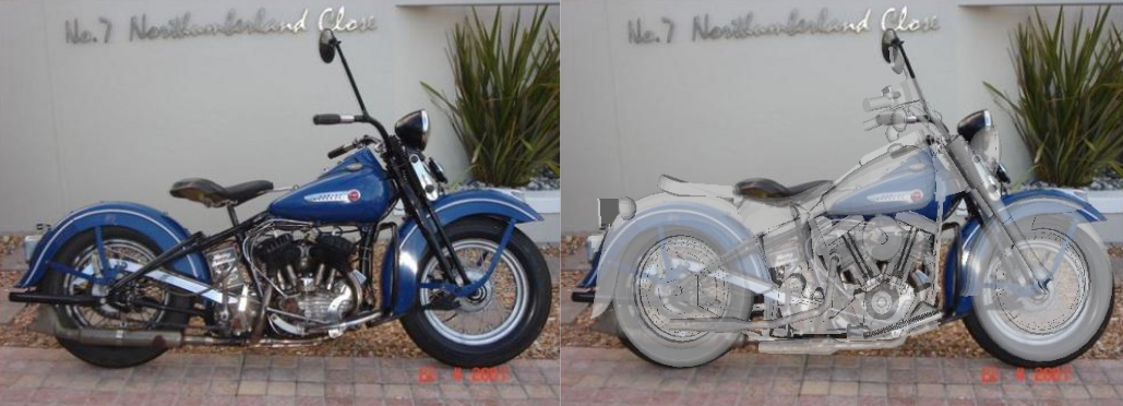
(f) Pose OOD, Motorbike

Figure 3: Qualitative results of RCNet on Occluded PASCAL3D+ and OOD-CV (a-f). We illustrate the predicted 3D pose using a CAD model. Note that the CAD model is not used in our approach.

4.2 Robust 3D-Aware Object Classification

We evaluate the performance on classification, 3D pose estimation, and 3D-aware classification separately on three datasets: PASCAL3D+ containing images without occlusion, Occluded PASCAL3D+ measuring the robustness under different occlusion levels, and OOD-CV measuring the robustness under different nuisances.

Performance in IID scenarios. The typical way of estimating the performance of an algorithm is to evaluate its performance on similarly distributed data, i.e., independently and identically distributed data (IID). We observe that our RCNet outperforms all baselines by a large margin at pose estimation and 3D-aware classification (+2.3 and +5.4 percent points on average compared to the best baseline, respectively). Furthermore, it matches the classification performance (shown in Table 2) of classical deep networks, which are all higher than 99%.

Performance in OOD scenarios. We evaluate our model in various OOD scenarios in Table 2. We note that RCNet outperforms all baselines by a considerable margin for classification, especially in high occlusion levels and across all nuisances in the OOD-CV dataset.

For 3D pose estimation (Table 2), RCNet considerably outperforms the feed-forward approaches. Moreover, it achieves a comparable performance (less than 2% lower) compared to NeMo, which is specifically designed for robust 3D pose estimation. However, on the OOD-CV dataset, RCNet consistently outperforms NeMo for all nuisance factors. This indicates that the discriminatively trained neural textures not just benefit the classification performance but also enhance the pose estimation in OOD scenarios. On average, our results for pose estimation are consistently the best compared to feed-forward networks. Noticeably, RCNet performs $60\%$ better than the best baseline at $\frac{\pi}{18}$ accuracy on the OOD-CV dataset.

From Table 4, we can observe that RCNet outperforms all baselines at 3D-aware object classification in OOD scenarios across all nuisance factors with a significant performance gap. Remarkably, RCNet achieves the best results at 3D-aware classification on IID and OOD scenarios.

Figure 3 shows qualitative examples of our proposed model on the occluded-PASCAL3D+ and OOD-CV datasets. Note how RCNet can robustly estimate 3D poses for objects in various out-of-distribution scenarios.

4.3 Efficient Scaling

We seek to reduce the computational cost of our method while retaining the performance and robustness as much as possible. Hence, we evaluate our scaling approach using two metrics: computational cost reduction and accuracy. We analyze the effect of each component of our scaling strategy separately in the following.

Step 1: Handle simple cases with CNNs ($S_{1}$). We define the threshold $\tau_{1}$ experimentally to maximize the true positives, i.e., the feed-forward model predicts the correct category with high confidence, while minimizing the false positives, i.e., the feed-forward model predicts the wrong category with high confidence. It allows us to reduce the processing requirements by $28\%$ overall and by $75\%$ for the unoccluded subset. This significant speedup has a minor downside: an average false positive rate of $0.2\%$. Hence, we expect a slight drop in accuracy (Table 4 shows a drop slightly lower than expected due to rounding errors).

Step 2: Propose-and-verify with CNN output ($S_{2}$). Compared to the naïve approach, using the feed-forward predictions as initialization reduces computation by a factor of 4 overall. Furthermore, it is interesting to note that our proposed initialization scheme is very beneficial in unoccluded cases and leads to an improvement of more than $2\%$ in accuracy (see Table 4 for more details). We do not observe a performance gain for occluded images, which provides further evidence that feed-forward models are less reliable in OOD scenarios. Compared to the naïve approach, this effective initialization reduces computation by a factor of 4.

Step 3: Full render-and-compare when uncertain ($S_{3}$). In some cases, the render-and-compare optimization does not converge to a good solution. These correspond to $19\%$ of all images (occluded and unoccluded) and around $1\%$ in unoccluded cases. This happens either due to the top-3 class prediction not including the ground-truth class or a sub-optimal estimation of the initialization pose parameters. By applying a threshold on the reconstruction loss, we can recover $92\%$ of these wrong predictions. While this step leads to a significantly increased computation in such hard cases, it enables RCNet to recover most of the wrong predictions that the feed-forward models make. Similarly to $\tau_{1}$, $\tau_{2}=0.8$ is fixed experimentally. It is interesting to note how each threshold influences results, and although we fixed these thresholds experimentally, they also generalize well for OOD data, as shown in Table 4.

In short, we introduce a principled approach to reduce the computational cost of render-and-compare approaches while retaining most of the performance and robustness of RCNet. Moreover, a synergistic effect is observed in many situations, leading to improved performance when combining standard models with render-and-compare approaches.

5 Conclusion

In this work, we studied the problem of 3D-aware object classification, i.e., simultaneously estimating the object class and its 3D pose. We observed that feed-forward neural networks and render-and-compare approaches lack performance and robustness at 3D-aware classification. Following this observation, we made three contributions:

Render-and-Compare-Net (RCNet). We introduced a 3D-aware neural network architecture representing objects as cuboid meshes with discriminatively trained neural textures. RCNet performs classification and pose estimation in a unified manner through inverse rendering, enabling it to perform exceptionally well at 3D-aware classification.

Efficient Scaling of Render-and-Compare. We integrated a feed-forward neural network into the render-and-compare process of RCNet in a principled manner to reach a sweet spot that further enhances the performance while also greatly reducing the computational cost at inference time.

Out-of-distribution Robustness. We observed that RCNet is exceptionally robust in out-of-distribution scenarios, such as when objects are partially occluded or seen in a new texture, pose, context, shape, or weather.

Supplementary material

We provide additional results and discussions to support the experimental results in the main paper. We study in more details the influence and sensitivity of our experimentally fixed thresholds on the results in this section.

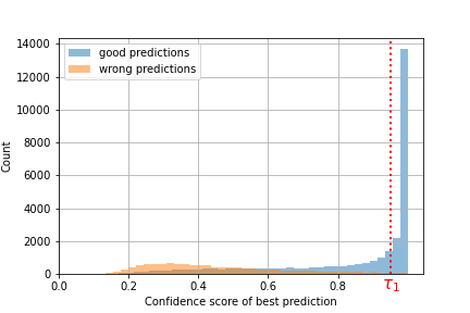
(a) Distribution of feed-forward’s confidence outputs for samples that correctly and wrongly predict the object’s category after $S_{1}$. Here, we take the prediction as is only when confidence is higher than the threshold $\tau_{1}=0.95$.

(b) ROC curve for CNN predictions.
We represent the threshold $\tau_{1}=0.95$.

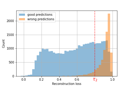
(c) Distribution of reconstruction loss values for samples that correctly and wrongly predict the object’s category after $S_{2}$. Here, we move forward to $S_{3}$ when the loss is higher than the threshold $\tau_{2}=0.8$.

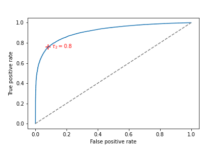
(d) ROC curve for reconstruction loss.
We represent the threshold $\tau_{2}=0.8$.

Figure S1: Illustration of scores distribution after steps $S_{1}$ (Figure 1(a)) and $S_{2}$ (Figure 1(c)) and their corresponding receiver operating characteristic (ROC) curves (Figures 1(b) and 1(d), respectively)

Appendix A Sensitivity to thresholds

We introduced in Section 3.4 a principled manner of enhancing the performance while also greatly reducing the computational cost at inference time. However this procedure relies on a couple of hyperparameters $\tau_{1}$ (in $S_{1}$) and $\tau_{2}$ (in $S_{3}$). Since these thresholds have been fixed from experimental results, we are interested to see if they generalize well and that their influence on the results is not significant. Due to the constraint on the definition domain of our metrics (in the interval $\left[0,1\right]$), we reduced the range of the sensitivity analysis according to the proximity to 1 (i.e., $\tau_{1}=0.95\pm 0.025$ and $\tau_{2}=0.8\pm 0.1$).

Metric	$ACC_{\frac{\pi}{6}}\uparrow$					$ACC_{\frac{\pi}{18}}\uparrow$					Computation cost $\downarrow$ (in % of the reference)
Nuisance	L0	L1	L2	L3	Mean	L0	L1	L2	L3	Mean	L0	L1	L2	L3	Mean
Ours	85.8	73.8	57.0	30.8	61.9	61.5	42.6	26.6	10.6	35.3	100	100	100	100	100
Ours$+$Scaling with $\tau_{1}^{\uparrow}$	89.6	77.3	60.0	32.0	65.3	65.0	44.7	28.1	11.3	37.9	12	44	75	106	59
Ours$+$Scaling with $\tau_{1}^{\downarrow}$	89.7	77.2	59.9	32.1	65.3	65.0	44.5	28.1	11.3	37.8	11	42	75	106	57
Ours$+$Scaling with $\tau_{2}^{\uparrow}$	89.7	71.8	51.5	24.4	60.0	65.0	42.6	25.3	9.3	36.2	11	42	69	99	54
Ours$+$Scaling with $\tau_{2}^{\downarrow}$	89.6	77.3	60.0	32.1	65.4	64.2	44.5	28.1	11.2	37.6	12	45	77	111	61
Ours$+$Scaling	89.7	77.2	60.0	32.1	65.4	65.0	44.7	28.1	11.2	37.8	12	44	75	106	59

Table S1: Study of the sensitivity of our scaling approach at 3D-aware classification on the (Occluded) PASCAL3D+ dataset. Ours refers to RCNet described in 3.3. Ours+Scaling refers to the full combination of RCNet and the feed-forward model as described in 3.4. We use the following values for the different thresholds: $\tau_{1}=0.95\pm 0.025$ and $\tau_{2}=0.8\pm 0.1$.

A.1 Sensitivity to feed-forward confidence threshold $\tau_{1}$

To assess the sensitivity of the results to the threshold $\tau_{1}$ that is used in $S_{1}$, we study the results with different threshold values. By increasing $\tau_{1}$, we expect the feed-forward network to help in classifying correctly objects during $S_{1}$ in fewer cases, thus, leading to increased computation and similar accuracy. We foresee a similar accuracy given that all missed first-shot classification would be recovered during $S_{2}$. By decreasing $\tau_{1}$, we expect an increase in the false positive rate (FPR), as illustrated in Figure 1(b). A higher FPR would translate to a lower accuracy and a lower computation. Table S1 shows that all assumptions can be verified experimentally. We used $\tau_{1}=0.975$ and $\tau_{1}=0.925$ ($\pm 3\%$ compared to the original threshold) when referring to $\tau_{1}^{\uparrow}$ and $\tau_{1}^{\downarrow}$, respectively. However, we do not observe a higher computation cost when increasing $\tau_{1}$, to observe that we would have to increase it to a higher value (i.e., 0.99).

Finally, as is to be expected in theory, the accuracy is not affected by a large margin when increasing the threshold $\tau_{1}$. However, decreasing it increases the false positives and reduces the accuracy by the same amount.

A.2 Sensitivity to reconstruction loss threshold $\tau_{2}$

During $S_{3}$, we seek to recover objects that were wrongly classified or with the wrong pose in previous steps. The reconstruction error gives a good intuition on the quality of the outcome. Hence, by increasing $\tau_{2}$, we assume that fewer wrong estimations from feed-forward suggestions will be recovered and thus, we expect a drop in the performance and computation. On the opposite, by decreasing $\tau_{2}$ we expect similar performances but a higher computation requirement since it involves using the most computational approach for objects already correctly classified and with the correct estimated pose. Table S1 validates experimentally previous theoretical statements. We used $\tau_{2}=0.7$ and $\tau_{2}=0.9$ ($\pm 12\%$ compared to the original threshold) when referring to $\tau_{2}^{\uparrow}$ and $\tau_{2}^{\downarrow}$, respectively. Nonetheless, we observe that when increasing $\tau_{2}$, accuracy reduces for strong occlusions cases. That can be explained by the fact that increasing $\tau_{2}$ increases the influence of the feed-forward model, which is not reliable in occluded cases, on the results

Hence, we establish experimentally that the threshold $\tau_{2}$ does not have a strong influence on the results. Since $\tau_{2}$ balances the importance between the feed-forward and the generative approaches, we need to find an optimal sweet spot to balance the shortcomings of each approach.

A.3 Discussion

From these results, we see that all our results are consistent with what has been shown in Section 4.3 of the main paper. By changing $\tau_{1}$ and $\tau_{2}$ by $\pm 3\%$ and $\pm 12\%$, respectively, we observe a maximum change in the overall results by $0.2\%$ and $8.2\%$, respectively. Although there are some minor differences in the results, we observe that all claims that have been made in the paper still stand with different thresholds. Thus, we can affirm that our results generalize well and that a change in thresholds gives similar results.

References

- [1] Yutong Bai, Angtian Wang, Adam Kortylewski, and Alan Yuille. Coke: Localized contrastive learning for robust keypoint detection. arXiv preprint arXiv:2009.14115, 2020.
- [2] Eran Borenstein and Shimon Ullman. Combined top-down/bottom-up segmentation. IEEE Trans. Pattern Anal. Mach. Intell., 30(12):2109–2125, Dec. 2008.
- [3] Ekin D Cubuk, Barret Zoph, Dandelion Mane, Vijay Vasudevan, and Quoc V Le. Autoaugment: Learning augmentation policies from data. arXiv preprint arXiv:1805.09501, 2018.
- [4] Alexey Dosovitskiy, Lucas Beyer, Alexander Kolesnikov, Dirk Weissenborn, Xiaohua Zhai, Thomas Unterthiner, Mostafa Dehghani, Matthias Minderer, Georg Heigold, Sylvain Gelly, et al. An image is worth 16x16 words: Transformers for image recognition at scale. arXiv preprint arXiv:2010.11929, 2020.
- [5] Yarin Gal et al. Uncertainty in deep learning. 2016.
- [6] Ulf Grenander. A unified approach to pattern analysis. In Advances in computers, volume 10, pages 175–216. Elsevier, 1970.
- [7] Kaiming He, Xiangyu Zhang, Shaoqing Ren, and Jian Sun. Deep residual learning for image recognition. In Proceedings of the IEEE conference on computer vision and pattern recognition, pages 770–778, 2016.
- [8] Dan Hendrycks, Norman Mu, Ekin D Cubuk, Barret Zoph, Justin Gilmer, and Balaji Lakshminarayanan. Augmix: A simple data processing method to improve robustness and uncertainty. arXiv preprint arXiv:1912.02781, 2019.
- [9] Dan Hendrycks, Kevin Zhao, Steven Basart, Jacob Steinhardt, and Dawn Song. Natural adversarial examples. In Proceedings of the IEEE/CVF Conference on Computer Vision and Pattern Recognition, pages 15262–15271, 2021.
- [10] Shun Iwase, Xingyu Liu, Rawal Khirodkar, Rio Yokota, and Kris M Kitani. Repose: Fast 6d object pose refinement via deep texture rendering. In Proceedings of the IEEE/CVF International Conference on Computer Vision, pages 3303–3312, 2021.
- [11] Shun Iwase, Xingyu Liu, Rawal Khirodkar, Rio Yokota, and Kris M. Kitani. Repose: Fast 6d object pose refinement via deep texture rendering. In Proceedings of the IEEE/CVF International Conference on Computer Vision (ICCV), pages 3303–3312, October 2021.
- [12] Adam Kortylewski, Ju He, Qing Liu, and Alan L. Yuille. Compositional convolutional neural networks: A deep architecture with innate robustness to partial occlusion. In Proceedings of the IEEE/CVF Conference on Computer Vision and Pattern Recognition (CVPR), June 2020.
- [13] Adam Kortylewski, Qing Liu, Huiyu Wang, Zhishuai Zhang, and Alan Yuille. Combining compositional models and deep networks for robust object classification under occlusion. In Proceedings of the IEEE/CVF Winter Conference on Applications of Computer Vision, pages 1333–1341, 2020.
- [14] Victor A. F. Lamme, Hans Supèr, and Henk Spekreijse. Feedforward, horizontal, and feedback processing in the visual cortex. Curr. Opin. Neurobiol., 8(4):529–535, Aug. 1998.
- [15] Yann LeCun, Yoshua Bengio, et al. Convolutional networks for images, speech, and time series. The handbook of brain theory and neural networks, 3361(10):1995, 1995.
- [16] Ze Liu, Yutong Lin, Yue Cao, Han Hu, Yixuan Wei, Zheng Zhang, Stephen Lin, and Baining Guo. Swin transformer: Hierarchical vision transformer using shifted windows. In Proceedings of the IEEE/CVF International Conference on Computer Vision, pages 10012–10022, 2021.
- [17] J. H. Maunsell and W. T. Newsome. Visual processing in monkey extrastriate cortex. Annu. Rev. Neurosci., 10(363-401.):;, 1987.
- [18] Arsalan Mousavian, Dragomir Anguelov, John Flynn, and Jana Kosecka. 3d bounding box estimation using deep learning and geometry. In Proceedings of the IEEE conference on Computer Vision and Pattern Recognition, pages 7074–7082, 2017.
- [19] Stephen E Palmer. Vision science: Photons to phenomenology. MIT press, 1999.
- [20] Sandro Schönborn, Andreas Forster, Bernhard Egger, and Thomas Vetter. A monte carlo strategy to integrate detection and model-based face analysis. In German Conference on Pattern Recognition, pages 101–110. Springer, 2013.
- [21] Karen Simonyan and Andrew Zisserman. Very deep convolutional networks for large-scale image recognition. arXiv preprint arXiv:1409.1556, 2014.
- [22] Zhuowen Tu, Xiangrong Chen, Yuille, and Zhu. Image parsing: unifying segmentation, detection, and recognition. In Proceedings Ninth IEEE International Conference on Computer Vision, pages 18–25 vol.1, 2003.
- [23] Shubham Tulsiani and Jitendra Malik. Viewpoints and keypoints. In Proceedings of the IEEE Conference on Computer Vision and Pattern Recognition, pages 1510–1519, 2015.
- [24] Ashish Vaswani, Noam Shazeer, Niki Parmar, Jakob Uszkoreit, Llion Jones, Aidan N Gomez, Łukasz Kaiser, and Illia Polosukhin. Attention is all you need. Advances in neural information processing systems, 30, 2017.
- [25] Angtian Wang, Adam Kortylewski, and Alan Yuille. Nemo: Neural mesh models of contrastive features for robust 3d pose estimation. In International Conference on Learning Representations, 2021.
- [26] Angtian Wang, Shenxiao Mei, Alan L Yuille, and Adam Kortylewski. Neural view synthesis and matching for semi-supervised few-shot learning of 3d pose. Advances in Neural Information Processing Systems, 34:7207–7219, 2021.
- [27] Angtian Wang, Yihong Sun, Adam Kortylewski, and Alan L Yuille. Robust object detection under occlusion with context-aware compositionalnets. In Proceedings of the IEEE/CVF Conference on Computer Vision and Pattern Recognition, pages 12645–12654, 2020.
- [28] Yu Xiang, Roozbeh Mottaghi, and Silvio Savarese. Beyond pascal: A benchmark for 3d object detection in the wild. In IEEE Winter Conference on Applications of Computer Vision (WACV), 2014.
- [29] Yu Xiang, Roozbeh Mottaghi, and Silvio Savarese. Beyond pascal: A benchmark for 3d object detection in the wild. In IEEE winter conference on applications of computer vision, pages 75–82. IEEE, 2014.
- [30] Amir R Zamir, Alexander Sax, Nikhil Cheerla, Rohan Suri, Zhangjie Cao, Jitendra Malik, and Leonidas J Guibas. Robust learning through cross-task consistency. In Proceedings of the IEEE/CVF Conference on Computer Vision and Pattern Recognition, pages 11197–11206, 2020.
- [31] Bingchen Zhao, Shaozuo Yu, Wufei Ma, Mingxin Yu, Shenxiao Mei, Angtian Wang, Ju He, Alan Yuille, and Adam Kortylewski. Ood-cv: A benchmark for robustness to individual nuisances in real-world out-of-distribution shifts. In Proceedings of the European Conference on Computer Vision (ECCV), 2022.
- [32] Xingyi Zhou, Arjun Karpur, Linjie Luo, and Qixing Huang. Starmap for category-agnostic keypoint and viewpoint estimation. In Proceedings of the European Conference on Computer Vision (ECCV), pages 318–334, 2018.