Two Matrix Model, the Riemann Hypothesis
and Master Matrix Obstruction

Abstract

We identify the Riemann Xi function as the Baker-Akhiezer function for a $(p,1)$ two matrix model as $p$ goes to infinity. We solve the two matrix model using biorthogonal polynomials and study the zeros of the polynomials in the double scaling limit as $N$ goes to infinity. We find zeros off the critical line at finite $N$ which possibly go to infinity as $N$ goes to infinity. We study other Baker-Akhiezer functions whose zeros are known to be on a critical line using the two matrix model technique and find the zeros on the critical line in those cases. We study other L-functions using the two matrix model and compare the biorthogonal method with other approaches to the two matrix model such as the master matrix approach and saddle point method. In cases where there are zeros off the critical line the master matrix approach encounters an obstruction to the solution to a quenched master matrix.

1 Introduction

The Riemann hypothesis, which states that the zeros of the Riemann zeta function lie on the critical line, continues to intrigue and attract mathematicians and physicists alike [1] [2] [3] [4] [5] [6]. There are indications that the hypothesis is related to quantum mechanics, although it appeared in the the nineteenth century, well before quantum mechanics had been formulated. In addition the spacing of the zeros have distributions in common with random matrix integrals. In this paper we explore a different connection of the Riemann hypothesis and quantum mechanics through its relation to the $(p,1)$ two matrix model in the limit where $p$ and the size of the matrix $N$ goes to infinity. Here $p$ refers to the degree of the potential of one of the matrices in the two matrix model with the other matrix having a degree $1$ or linear potential. The relation will allow us to relate the Riemann Xi function to the Baker-Akhiezer of the two matrix model and study its zeros using the biorthogonal polynomial method of solution.

This paper is organized as follows. In section 2 we review some basic facts about the Riemann Xi function and its representation as a Fourier integral. In section 3 we review some features of the two matrix model needed for this paper and how the representation of the Baker-Akhiezer function as a Fourier integral leads to a connection to the Riemann Xi function [7] [8]. In section 4 we apply the method of biorthogonal polynomials [9] [10] to the study of the simplest case, the $(2,1)$ two matrix model, whose Baker-Akhiezer function is the Airy function and show how to obtain the zeros as the zeros of a polynomial. In section 5 we apply the same method to the Riemann Xi function, except in that case we find zeros off the critical line which possibly go to infinity as $p$ and $N$ go to infinity. In section 6 we apply the method to other L functions such as the Ramanujan L function and also see zeros off the critical line which also may go to infinity in the double scaling limit. In section 7 we discuss Baker-Akhiezer function which are know to have zeros on critical lines and show in those cases the two matrix model also yields zeros on the critical line. In section 8 we discuss the $p$ goes to infinity limit in a case where the polynomial expansion of the potential is particularly straightforward again finding zeros on the corresponding critical line. In section 9 we discuss other methods to solve the two matrix model besides the biorthogonal polynomial method such as the master matrix and saddle point method. In the case of the master matrix method we find an obstruction to the solution of the master matrix when some zeros are off the critical line. Finally in section 10 we discuss our conclusions and directions for future work.

2 Review of Riemann Xi function

The Riemann Xi function is defined as

$$\Xi(z)=\xi(\frac{1}{2}+iz)$$ (2.1)

where

$$\xi(s)=\frac{1}{2}s(s-1){\pi^{-s/2}}\Gamma(s/2)\zeta(s)$$ (2.2)

It shares all the nontrivial zeros of the Riemann zeta function but does not have the pole or the trivial zeros. It can be represented as a Fourier integral as:

$$\psi_{R}(z)=\Xi(z)=\int_{-\infty}^{\infty}{\Phi(x){e^{ixz}}dx}$$ (2.3)

where

$$\Phi(x)=\sum\limits_{n=1}^{\infty}{\left({4{\pi^{2}}{n^{4}}{e^{9x/2}}-6\pi{n^{2}}{e^{5x/2}}}\right)}\exp\left({-\pi{n^{2}}{e^{2x}}}\right)$$ (2.4)

with derivative:

$$\Phi^{\prime}(x)=\sum\limits_{n=1}^{\infty}{\left({30{\pi^{2}}{n^{4}}{e^{9x/2}}-15\pi{n^{2}}{e^{5x/2}}-8{\pi^{3}}{n^{6}}{e^{13x/2}}}\right)}\exp\left({-\pi{n^{2}}{e^{2x}}}\right)$$ (2.5)

For connections to the $(p,1)$ two matrix model one can also form the series:

$$U(x)=-\log\left({\Phi(x)}\right)=\sum\limits_{n=0}^{\infty}{{a_{n}}{x^{n}}}$$ (2.6)

and the truncated version at order $p+1$ given by:

$${U_{p}}(x)=\sum\limits_{n=0}^{p+1}{{a_{n}}{x^{n}}}$$ (2.7)

It is convenient to rescale the term of order $p+1$ so its coefficient is given by $1/(p+1)$. Then we have:

$${U_{p}}\left({\frac{{\bar{x}}}{{{{\left({{a_{p+1}}\left({p+1}\right)}\right)}^{1/(p+1)}}}}}\right)=\frac{{{{\bar{x}}^{p+1}}}}{{p+1}}+\sum\limits_{n=2}^{p-1}{{s_{n-1}}{{\frac{{\bar{x}}}{n}}^{n}}}+a_{0}$$ (2.8)

where:

$${s_{n-1}}=n{a_{n}}\frac{1}{{{{\left({{a_{p+1}}\left({p+1}\right)}\right)}^{n/(p+1)}}}}$$ (2.9)

The Baker-Akhiezer representation of the Riemann Xi function is then:

$${\psi_{R}}(z)=\Xi(z)={\lim_{p\to\infty}}\int_{-\infty}^{\infty}{{e^{-{U_{p}}(x)}}{e^{izx}}dx}$$ (2.10)

which as we shall see is the limit of the expectation value of the characteristic polynomial for the $(p,1)$ two matrix model as $p$ goes to infinity.

3 Review $(p,1)$ two matrix model

We will mainly follow the approach to the $(p,1$ two matrix model in [11] [12]. Many aspects two matrix model have been developed in the physics [13-77] and mathematics literature [78-84]. The partition function for the $(p,1)$ two matrix model is given by

$$Z=\int{dAdB{e^{-\frac{1}{g}Tr(V(A)+B-AB)}}}$$ (3.1)

where $A$ and$B$ are two Hermitian $N\times N$ matrices, $V(A)$ is the potential for the $A$ matrix and $B$ is the potential for the $B$ matrix. After shifting $A$ by the identity the partition function becomes:

$$Z=\int{dAdB{e^{-\frac{1}{g}Tr(V(A+I)-AB)}}}$$ (3.2)

The quantity that interests us is the expectation value of the characteristic polynomial of the $B$ matrix given by:

$$\left\langle{\det(b-B)}\right\rangle=\int{dAdB{e^{-\frac{1}{g}Tr(V(A+I)-AB)}}\det(b-B)}$$ (3.3)

The expectation value of the characteristic polynomial of $B$ can be computed using biorthogonal polynomials $P_{m}(a),Q_{n}(b)$ which obey

$$\int{dadb{P_{m}}}(a){Q_{n}}(b){e^{-\frac{1}{g}\left({V(a+1)-ab)}\right)}}={h_{m}}{\delta_{m,n}}$$ (3.4)

The biorthogonal polynomials are given as:

$${P_{m}}(a)={a^{m}}$$

$${Q_{n}}(b)={\left({-g\frac{\partial}{{\partial a}}}\right)^{n}}{\left.{\left({{e^{-\frac{1}{g}\left({V(a+1)-ab)}\right)}}}\right)}\right|_{a=0}}$$ (3.5)

And the expectation value of the characteristic polynomial can be shown to be:

$$\left\langle{\det(b-B)}\right\rangle={Q_{N}}(b)={\left({-g\frac{\partial}{{\partial a}}}\right)^{N}}{\left.{\left({{e^{-\frac{1}{g}\left({V(a+1)-ab)}\right)}}}\right)}\right|_{a=0}}$$ (3.6)

To obtain the Baker-Akhiezer function we take the double scaling limit where the potential $V(A)$ is a $p$ degree matrix polynomial of the form:

$$V(A)={V_{p}}(A)+{s_{1}}{\epsilon^{p-1}}{V_{1}}(A)+{s_{3}}{\epsilon^{p-2}}{V_{3}}(A)+\ldots+{s_{p-2}}{\epsilon^{2}}{V_{p-2}}(A)$$ (3.7)

where:

$${V_{n}}(A)=-\sum\limits_{k=1}^{n}{\left({\frac{{{A^{k}}}}{k}-\frac{I}{k}}\right)}$$ (3.8)

and

$$\epsilon=\left(\frac{1}{N}\right)^{\frac{1}{p+1}}$$

$$g=\frac{1}{N}+\frac{1}{N}\left({{\epsilon^{2}}{s_{p-2}}+{\epsilon^{4}}{s_{p-4}}+\ldots+{\epsilon^{p-1}}{s_{1}}}\right)$$

$$a=-1+\epsilon x$$ (3.9)

Then taking the large $N$ limit as $\epsilon$ goes to zero one can express the expectation value of the characteristic polynomial as the Fourier integral

$$\psi(z)=\int_{-\infty}^{\infty}{{e^{-{U_{p}}(x)}}{e^{izx}}dx}$$ (3.10)

with $U_{p}(x)$ given by:

$${U_{p}}(x)=\frac{x^{p+1}}{p+1}+{s_{1}}\frac{{{x^{2}}}}{2}+{s_{1}}\frac{{{x^{4}}}}{4}\ldots+{s_{p-2}}\frac{{{x^{p-1}}}}{{p-1}}$$ (3.11)

which represents the Baker-Akhierzer function as a Fourier integral. In the following sections we will apply these formulas to the study of various functions such as the Riemann Xi function which be represented as the Baker-Akhiezer function of two matrix models.

If one defines the Jacobi Matrix $J_{M}$

$$x\frac{{{Q_{n}}(x)}}{{\sqrt{{h_{n}}}}}=\sum\limits_{m=0}^{n+1}{{(J_{M})_{n,m}}\frac{{{Q_{m}}(x)}}{{\sqrt{{h_{m}}}}}}$$ (3.12)

Then taking the $N\times N$ submatrix of $J_{M}$ yields:

$$\left\langle{\det(b-B)}\right\rangle=\det(b-J_{M})$$ (3.13)

one can also obtain the polynomials $Q_{n}(b)$ from the generating function:

$${e^{\frac{1}{g}V(gt+1)}}{e^{-yt}}=\sum\limits_{N=1}^{\infty}{\frac{{{Q_{N}}(y){t^{N}}}}{{N!}}}$$ (3.14)

4 Two Matrix Model and Airy function zeros

The $(2,1)$ Matrix model was studied in [12]. Because $p=2$ the derivative formula for the $Q_{n}(b)$ polynomials reduces to the Hermite polynomials and the expectation value of the characteristic polynomial is given by:

$$\left\langle{\det\left({b-B}\right)}\right\rangle={\left({\frac{g}{4}}\right)^{N/2}}{H_{N}}\left({b\frac{1}{{\sqrt{g}}}}\right)$$ (4.1)

For $N=16$ and $gN=1$ this leads to the polynomial:

$$Q_{16}(b)=b^{16}-3.75b^{14}+5.33203b^{12}- 3.66577b^{10}+1.28875b^{8}-0.225531b^{6}$$

$$+0.0176196b^{4}-0.000471954b^{2}+1.84357\times 10^{-6}$$ (4.2)

The zeros of the polynomial are:

$$b_{1}=-1.17218$$

$$b_{2}=-0.967362$$

$$b_{3}=-0.79425$$

$$b_{4}=-0.636551$$

$$b_{5}=-0.487947$$

$$b_{6}=-0.345065$$

$$b_{7}=-0.205738$$

$$b_{8}=-0.0683703$$

$$b_{9}=0.0683703$$

$$b_{10}=0.205738$$

$$b_{11}=0.345065$$

$$b_{12}=0.487947$$

$$b_{13}=0.636551$$

$$b_{14}=0.79425$$

$$b_{15}=0.967362$$

$$b_{16}=1.17218$$ (4.3)

The Baker-Akhiezer function for the $(2,1)$ two matrix model is the Airy function. The zeros of the polynomial are related to the Airy function $Ai(y)$ through a linear relation $y=Ab+c$. For

$$y=-8(2^{1/6})\left(\sqrt{2}-b\right)$$ (4.5)

the first three zeros are:

$$y_{1}=-8(2^{1/6})\left(\sqrt{2}-b_{16}\right)$$

$$y_{2}=-8(2^{1/6})\left(\sqrt{2}-b_{15}\right)$$

$$y_{3}=-8(2^{1/6})\left(\sqrt{2}-b_{14}\right)$$ (4.6)

yielding:

$$y_{1}=-2.17335$$

$$y_{2}=-4.01259$$

$$y_{3}=-5.56709$$ (4.7)

which can be compared to the exact value for Airy zeros given by -2.33811, -4.08795, -5.52056. One can obtain more accurate values of the Airy zeros from the polynomials by going to larger values of N as shown in figure 1 for $N=32$.

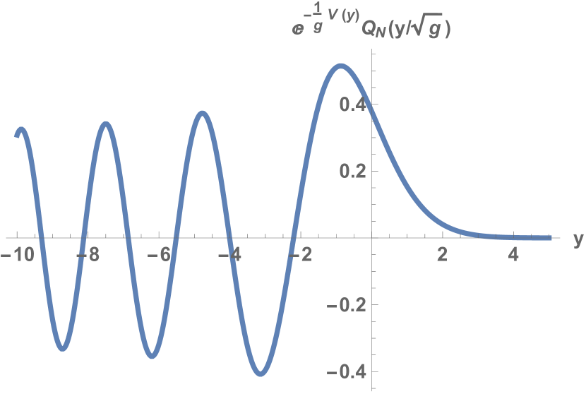
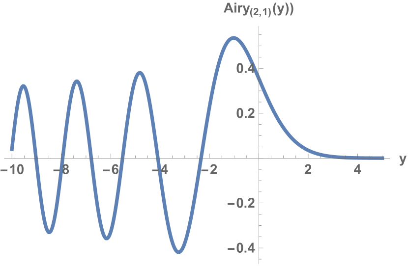
Figure 1: (left) Approximation to the Airy function from the $(2,1)$ two Matrix model with $N=32$. (right) Exact expression for the Airy function. The two Matrix model approximation gives a good estimate to the first five zeros for $N=32$.

5 Two Matrix Model and Riemann Xi function zeros

The logarithm of the Phi function has the expansion

$$-\log(\Phi(x))=\sum\limits_{n=0}^{\infty}{{a_{n}}{x^{n}}}={a_{0}}+{a_{2}}{x^{2}}+{a_{4}}{x^{4}}+{a_{6}}{x^{6}}+{a_{8}}{x^{8}}+\ldots$$ (5.1)

working with the sum at the eighth order we have:

$$a_{0}=0.112728$$

$$a_{2}=9.3634$$

$$a_{4}=5.95896$$

$$a_{6}=-2.09194$$

$$a_{8}=3.53296$$ (5.2)

then using the expansion:

$${U_{p}}(\bar{x})=\frac{{{{\bar{x}}^{p+1}}}}{{p+1}}+{s_{1}}\frac{{{{\bar{x}}^{2}}}}{2}+{s_{3}}\frac{{{{\bar{x}}^{4}}}}{2}\ldots+{s_{p-1}}\frac{{{{\bar{x}}^{p-1}}}}{2}$$ (5.3)

for $p=7$ we obtain the $s_{n}$ coefficients for the corresponding $(7,1)$ two matrix model as:

$$s_{1}=8.12192$$

$$s_{4}=4.48349$$

$$s_{6}=-1.02395$$ (5.4)

Then using formulas (3.5) and (3.9) we have for the $N=16$ Q polynomial for $p=7$:

$$Q_{16}[b]=b^{16} +141.088b^{15}+8952.1b^{14}+338149.b^{13}+8.48406\times 10^{6}b^{12}$$

$$+1.49383\times 10^{8}b^{11}+1.90155\times 10^{9}b^{10}+1.77654\times 10^{10}b^{9}+1.2243\times 10^{11}b^{8}$$

$$+6.20423\times 10^{11}b^{7}+2.28714\times 10^{12}b^{6}+6.01787\times 10^{12}b^{5}+1.09783\times 10^{13}b^{4}$$

$$+1.33068\times 10^{13}b^{3}+1.00497\times 10^{13}b^{2}+4.23563\times 10^{12}b+7.61563\times 10^{11}$$ (5.5)

The polynomial zeros are given by:

$$b_{1}=-22.8352$$

$$b_{2}=-19.7169$$

$$b_{3}=-17.2138$$

$$b_{4}=-15.0434$$

$$b_{5}=-13.0978$$

$$b_{6}=-11.322$$

$$b_{7}=-9.68381$$

$$b_{8}=-8.16324$$

$$b_{9}=-6.74774$$

$$b_{10}=-5.43011$$

$$b_{11}=-4.20771$$

$$b_{12}=-3.08255$$

$$b_{13}=-2.0612$$

$$b_{14}=-1.12636$$

$$b_{15}=-0.677917-0.213125i$$

$$b_{16}=-0.677917+0.213125i$$ (5.6)

Fitting the first two zeros to the Riemann zeta zeros of the form $z_{i}=Ab_{i}+c$ we find $A=2.20867$ and $c=64.5702$ then the first three zeros determines by the polynomial zeros are $14.1347,21.022,26.5505$ which can be compared with the exact values $14.1347,21.022,25.0109$. One can increase the accuracy of the polynomial zero estimation of the zeros by going to larger $p$ and higher values of $N$. A plot of the Riemann Xi function which is the Baker Akheizer function for the two matrix model is shown in figure 2.

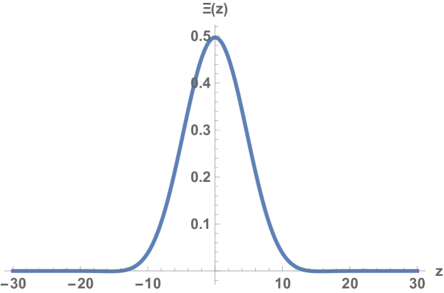
Figure 2: Plot of the Riemann Xi function which is the Baker Akheizer function for a two matrix model associated with the Riemann zeta function.

6 Two Matrix model and other L-function zeros

We can use the same two Matrix model technique to study other L-functions. For example the Ramanujan tau L function can be represented as a Fourier integral through:

$$\psi_{L}(z)={\Xi_{L}}(z)={(2\pi)^{-(6+iz)}}\Gamma(6+iz)L(6+iz)=\int_{-\infty}^{\infty}{{\Phi_{L}}(x){e^{ixz}}dx}$$ (6.1)

with $L$ the Ramanujan tau L function and:

$${\Phi_{L}}(x)={e^{-6x}}\Delta(i{e^{-x}})={e^{-6x}}{e^{-2\pi{e^{-x}}}}\prod\limits_{n=1}^{\infty}{{{\left({1-{e^{-2\pi n{e^{-x}}}}}\right)}^{24}}}$$ (6.2)

Defining:

$${\Phi_{L}}(x)=e^{-U_{L}(x)}$$ (6.3)

we find $U_{L}$ has an expansion out to eighth order given by :

$$U_{L}^{(8)}(x)=0.112629x^{8}-0.188291x^{6}+0.971962x^{4}+3.89463x^{2}+6.32813$$ (6.4)

so:

$$a_{0}=6.32813$$

$$a_{2}=3.89463$$

$$a_{4}=0.971962$$

$$a_{6}=-0.188291$$

$$a_{8}=0.112629$$ (6.5)

and these determine the parameters of the $(7,1)$ two Matrix model to be:

$$s_{1}=7.99487$$

$$s_{3}=4.0958$$

$$s_{5}=-1.22159$$ (6.6)

Using formula (3.5) for $N=16$ we obtain the polynomial

$$Q_{16}(b)= b^{16}+128.276b^{15}+7359.58b^{14}+249796.b^{13}+5.59101\times 10^{6}b^{12}$$

$$+8.70867\times 10^{7}b^{11}+9.7108\times 10^{8}b^{10}+7.8558\times 10^{9}b^{9}+4.62396\times 10^{10}b^{8}$$

$$+1.9692\times 10^{11}b^{7}+5.98673\times 10^{11}b^{6}+1.27226\times 10^{12}b^{5}+1.83727\times 10^{12}b^{4}$$

$$+1.74238\times 10^{12}b^{3}+1.04129\times 10^{12}b^{2}+3.62215\times 10^{11}b+5.49926\times 10^{10}$$ (6.7)

The zeros of the polynomial are given by:

$$b_{1}=-21.6904$$

$$b_{2}=-18.6188$$

$$b_{3}=-16.1563$$

$$b_{4}=-14.0238$$

$$b_{5}=-12.115$$

$$b_{6}=-10.3756$$

$$b_{7}=-8.77408$$

$$b_{8}=-7.29079$$

$$b_{9}=-5.91364$$

$$b_{10}=-4.63575$$

$$b_{11}=-3.45447$$

$$b_{12}=-2.37033$$

$$b_{13}=-1.37913$$

$$b_{14}=-0.506603-0.513116i$$

$$b_{15}=-0.506603+0.513116i$$

$$b_{16}=-0.464347$$ (6.8)

Fitting the first two zeros to the Riemann zeta zeros of the form $z_{i}=Ab_{i}+c$ we find $A=1.52532$ and $c=42.3072$ then the first three zeros determined by the polynomial zeros are $9.22238,13.90755,17.6636$ which can be compared with the exact first three zeros of the Ramanujan L function which are given by $9.22238,13.90755,17.442777$. One can obtain better estimates for the zeros by going to higher values of $N$ and $p$. It would be interesting to study the behavior of the complex zeros as for large $N$ to see if they go to infinity under the double scaling limit. A plot of the Ramanujan Xi function which is the Baker Akheizer function for a two matrix model is shown in figure 3.

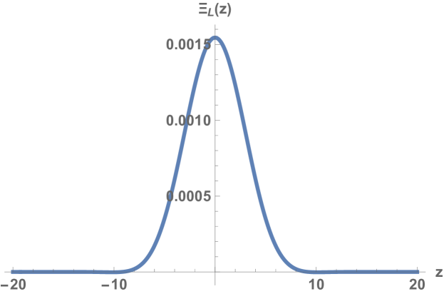
Figure 3: Plot of the Ramanujan Xi function which is the Baker Akheizer function for a two matrix model associated with the Ramnaujan L function.

7 Two Matrix Model and Baker-Akhiezer functions with zeros on the critical line

In [85] [86] [87] [88] [89] [90] [91] [92] [93] [94] [95] [96] [97] [98] several criteria were given that lead to Baker-Akhiezer functions with real zeros. If we express the Baker-Akhiezer function as a Fourier integral as:

$$\psi(z)=\int_{-\infty}^{\infty}{{e^{-U(x)}}{e^{izx}}dx}$$ (7.1)

then the the Baker-Akhiezer function will have real zeros if $U(x)$ is of the form:

$$U(x)=\frac{x^{2n}}{2n}$$ (7.2)

for $n>2$. Another case where Baker-Akhiezer functions with real zeros is when $U(x)$ is of the form:

$$U(x)=\frac{{{x^{4m}}}}{{2m}}+s_{2m-1}\frac{{{x^{2m}}}}{{2m}}+s_{1}\frac{{{x^{2}}}}{2}$$ (7.3)

with $s_{2m-1},s_{1}$ real $m=1,2,3,\dots$,2 with $s_{1}\leq 0$. Finally if $U(x)$ has a leading term $\frac{x^{2n}}{2n}$ and it’s value at imaginary arguments $U(iu)$ has real zeros only than the Baker-Akhiezer function will have real zeros.

An example of the first type above where $U(p)=\frac{x^{2n}}{2n}$ with $n=4$ and the Baker-Akhiezer function given by the generalized Airy function. Using formula (3.5) with $N=16$ we have the polynomial:

$$Q_{16}(b)= b^{16}+112.b^{15}+5722.5b^{14}+176798.b^{13}+3.69077\times 10^{6}b^{12}$$

$$+5.51006\times 10^{7}b^{11}+6.07273\times 10^{8}b^{10}+5.02779\times 10^{9}b^{9}+3.15136\times 10^{10}b^{8}$$

$$+1.49533\times 10^{11}b^{7}+5.33211\times 10^{11}b^{6}+1.40685\times 10^{12}b^{5}+2.67577\times 10^{12}b^{4}$$

$$+3.51786\times 10^{12}b^{3}+2.98205\times 10^{12}b^{2}+1.43339\times 10^{12}b+2.87152\times 10^{11}$$ (7.4)

with zeros give by:

$$b_{1}=-15.5108$$

$$b_{2}=-13.7506$$

$$b_{3}=-12.3194$$

$$b_{4}=-11.0623$$

$$b_{5}=-9.91975$$

$$b_{6}=-8.86087$$

$$b_{7}=-7.86714$$

$$b_{8}=-6.92631$$

$$b_{9}=-6.02971$$

$$b_{10}=-5.17091$$

$$b_{11}=-4.34496$$

$$b_{12}=-3.54788$$

$$b_{13}=-2.77634$$

$$b_{14}=-2.02742$$

$$b_{15}=-1.29834$$

$$b_{16}=-0.587221$$

Transforming these eigenvalues of the form $y=Ab+c$ these eigenvalues with $A=1.43304,c=24.7926$ we have the first three zeros as:

$$y_{1}=2.56503$$

$$y_{2}=5.08746$$

$$y_{3}=7.13834$$ (7.6)

defining:

$$Ai_{(7,1)}\left({y,{s_{1}},{s_{3}},{s_{5}}}\right)=\int_{-\infty}^{\infty}{dx{e^{-\left({{s_{1}}\frac{{{x^{2}}}}{2}+{s_{3}}\frac{{{x^{4}}}}{4}+{s_{5}}\frac{{{x^{6}}}}{6}+\frac{{{x^{8}}}}{8}}\right)}}}{e^{ixy}}$$ (7.7)

which can be compared to the first three zeros of $Ai_{(7,1)}(y)=Ai_{(7,1)}(y,0,0,0)$ given by $2.56503,5.08746,7.53357$. A plot of $Ai_{(7,1)}(y)$ showing the first few zeros is in in figure 4.

Figure 4: Plot of the generalized Airy function which is the Baker Akheizer function for the $(7,1)$ two matrix model showing the first few zeros.

For an example of the second type of $U(x)$ that yield a Baker-Akhiezer function that will have real zeros we will take:

$$U(x)=\frac{{{x^{8}}}}{8}+3\frac{{{x^{4}}}}{4}-\frac{{{x^{2}}}}{2}$$ (7.8)

so for this case:

$$s_{1}=-1$$

$$s_{3}=3$$

$$s_{5}=0$$ (7.9)

and for $N=16$ the polynomial representation of the expectation value of the characteristic polynomial is:

$$Q_{16}(b)= b^{16}+146.b^{15}+9708.52b^{14}+389701.b^{13}+1.05503\times 10^{7}b^{12}$$

$$+2.03871\times 10^{8}b^{11}+2.9022\times 10^{9}b^{10}+3.09666\times 10^{10}b^{9}+2.49541\times 10^{11}b^{8}$$

$$+1.51836\times 10^{12}b^{7}+6.92309\times 10^{12}b^{6}+2.32847\times 10^{13}b^{5}+5.62629\times 10^{13}b^{4}$$

$$+9.36259\times 10^{13}b^{3}+1.00052\times 10^{14}b^{2}+6.03675\times 10^{13}b+1.51162\times 10^{13}$$ (7.10)

whose zeros are:

$$b=-20.6811$$

$$b=-18.2512$$

$$b=-16.2823$$

$$b=-14.5587$$

$$b=-12.9977$$

$$b=-11.5564$$

$$b=-10.2094$$

$$b=-8.93992$$

$$b=-7.73641$$

$$b=-6.59062$$

$$b=-5.49659$$

$$b=-4.45016$$

$$b=-3.44881$$

$$b=-2.49194$$

$$b=-1.58201$$

$$b=-0.726718$$ (7.11)

Fitting the first two zeros to the generalized Airy zeros of the form $z_{i}=Ab_{i}+c$ we find $A=1.27473$ and $c=29.2615$ then the first three zeros determines by the polynomial zeros are $2.89881,5.99627,8.50607$ which can be compared with the exact values $2.89881,5.99627,8.6996$ for the first three zeros of $Ai_{(7,1)}(y,-1,3,0)$. One can increase the accuracy of the polynomial zero estimation of the zeros by going to higher values of $N$.

For an example of the third type of $U(x)$ that yield a Baker-Akhiezer function will have real zeros we will take:

$$U(x)=\frac{{{x^{8}}}}{8}+3\frac{{{x^{6}}}}{6}+3\frac{{{x^{4}}}}{4}+\frac{{{x^{2}}}}{2}$$ (7.12)

so that $U^{\prime}(iu)=0$ has solutions that are real. For this case:

$$s_{1}=1$$

$$s_{3}=3$$

$$s_{5}=3$$ (7.13)

and for $N=16$ the polynomial representation of the expectation value of the characteristic polynomial is:

$$Q_{16}(b)= b^{16}+270.b^{15}+33203.7b^{14}+2.46483\times 10^{6}b^{13}+1.23403\times 10^{8}b^{12}$$

$$+4.40938\times 10^{9}b^{11}+1.1605\times 10^{11}b^{10}+2.28877\times 10^{12}b^{9}+3.40782\times 10^{13}b^{8}$$

$$+3.82914\times 10^{14}b^{7}+3.22164\times 10^{15}b^{6}+1.99709\times 10^{16}b^{5}+8.87895\times 10^{16}b^{4}$$

$$+2.71163\times 10^{17}b^{3}+5.29656\times 10^{17}b^{2}+5.80173\times 10^{17}b+2.60471\times 10^{17}$$ (7.14)

whose zeros are given by:

$$b_{1}=-38.1637$$

$$b_{2}=-33.7063$$

$$b_{3}=-30.0921$$

$$b_{4}=-26.9256$$

$$b_{5}=-24.0553$$

$$b_{6}=-21.4028$$

$$b_{7}=-18.9211$$

$$b_{8}=-16.5794$$

$$b_{9}=-14.3561$$

$$b_{10}=-12.2356$$

$$b_{11}=-10.2064$$

$$b_{12}=-8.26003$$

$$b_{13}=-6.39036$$

$$b_{14}=-4.59403$$

$$b_{15}=-2.87196$$

$$b_{16}=-1.23928$$ (7.15)

Fitting the first two zeros to the generalized Airy zeros of the form $z_{i}=Ab_{i}+c$ we find $A=0.790259$ and $c=34.3341$ then the first three zeros determines by the polynomial zeros are $4.17486,7.69736,10.5535$ which can be compared with the exact values $4.17486,7.69736,10.9217$ for the first three zeros of $Ai_{(7,1)}(y,1,3,3)$. One can increase the accuracy of the polynomial zero estimation of the zeros by going to higher values of $N$.

8 Two Matrix models and the infinite $p$ limit

There has been recent interest in the infinite $p$ limit of two Matrix models. In [99] the $(p,2)$ two matrix model was used in the limit of infinite $p$ to study the $c\rightarrow\infty$ Liouville theory in the semiclassical limit. The coupled $(p,q)$ minimal matter model has central charge:

$$c=1-6\frac{{{{\left({p-q}\right)}^{2}}}}{{pq}}$$ (8.1)

which for the $(p,1)$ model yields:

$$c=1-6\left({p-2+\frac{1}{p}}\right)$$ (8.2)

which goes to $-\infty$ as $p$ goes to infinity. So the Liouvlle threory has central charge $+\infty$ so that the total theory plus ghosts is conformally invariant. The large $p$ limit allows one to use the semiclassical limit for the Liouville theory as in [99]. The large $p$ limit will also allow us to construct a two Matrix model which more accuractly computes the zeros of the Baker-Akhiezer function.

For the potential:

$$U(x)=\cosh\ (x)$$ (8.3)

we have the expansion:

$$\cosh(x)=\sum\limits_{n=0}^{\infty}{\frac{{{x^{2n}}}}{{\left({2n}\right)!}}}$$ (8.4)

So we can obtain exact expressions for the $s_{n}$ for the corresponding two matrix model. Only the odd $n$ are nonzero which take the value:

$${s_{2j+1}}=\frac{1}{{\left({2j+1}\right)!}}{\left({p!}\right)^{\frac{{2j+2}}{{p+1}}}}$$ (8.5)

for $2j+1=1,3,\ldots,p-2$.

The Baker-Akhiezer function associated with this $U(x)$ is the K-Bessel function

$${\psi(z)=K_{iz}}(1)=\int_{-\infty}^{\infty}{{e^{-\cosh x}}{e^{izx}}dx}$$ (8.6)

The potential for the two matrix model in this case

$$V(A,B)=Tr(\sum_{j=0}^{\frac{p-3}{2}}\frac{(p!)^{\frac{(2j+1)+1}{p+1}}\epsilon^{p-(2j+1)}V(2j+1,A+1)}{(2j+1)!}+V(p,A+1)-AB)$$ (8.7)

Because we have a closed form expressing for the potential as for arbitrary $p$ we can consider the large $p$ limit to closer approximate the zeros of Baker-Akhiezer function using the two matrix model. For $p=7$ and $N=16$ we have:

$$s_{1}=8.42573$$

$$s_{3}=11.8322$$

$$s_{5}=4.98473$$ (8.8)

and the $Q_{N}(b)$ polynomial is:

$$Q_{16}(b)= 1.b^{16}+470.227b^{15}+100563.b^{14}+1.29618\times 10^{7}b^{13}+1.12484\times 10^{9}b^{12}$$

$$+6.95391\times 10^{10}b^{11}+3.16015\times 10^{12}b^{10}+1.07377\times 10^{14}b^{9}+2.74766\times 10^{15}b^{8}$$

$$+5.29135\times 10^{16}b^{7}+7.60608\times 10^{17}b^{6}+8.02664\times 10^{18}b^{5}+6.04942\times 10^{19}b^{4}$$

$$+3.11591\times 10^{20}b^{3}+1.01997\times 10^{21}b^{2}+1.85683\times 10^{21}b+1.36908\times 10^{21}$$ (8.9)

with zeros given by:

$$b_{1}=-67.7171$$

$$b_{2}=-59.5952$$

$$b_{3}=-53.0264$$

$$b_{4}=-47.2861$$

$$b_{5}=-42.0962$$

$$b_{6}=-37.3136$$

$$b_{7}=-32.8525$$

$$b_{8}=-28.657$$

$$b_{9}=-24.6889$$

$$b_{10}=-20.9208$$

$$b_{11}=-17.3337$$

$$b_{12}=-13.9147$$

$$b_{13}=-10.6571$$

$$b_{14}=-7.56181$$

$$b_{15}=-4.64341$$

$$b_{16}=-1.96262$$ (8.10)

We can relate then zeros to the zeros of $K_{iz}(1)$ through a linear relation $z_{i}=Ab_{i}+c$ with $A=0.193542$ and $c=16.0687$. This can be used to obtain estimates the first three zeros as $2.96255,4.53449,5.80583$ with the first two fixed by the linear relation. This can be compared with the exact first three zeros of $K_{iz}(1)$ which are $2.96255,4.53449,5.87987$. A plot of $K_{iz}(1)$ showing the first few zeros is in figure 5.

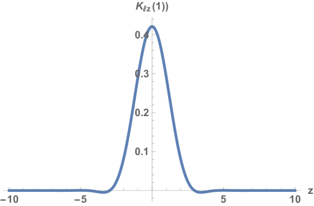
Figure 5: Plot of the Bessel $K_{iz}(1)$ function which is the Baker Akheizer function for the $(\infty,1)$ two matrix model.

It is also interesting in this case that

$$U^{\prime}(iu)=\sin(u)$$ (8.11)

only has real zeros so the third criteria for the Baker-Akhiezer function to have real zeros holds for this case too. Notably this seems to be true for the $U(x)$ functions associated with the Riemann Xi function and Ramanujan L-function. Those cases additionally have modular invariance properties. The function $U^{\prime}(x)$ has an additional interpretatation as a superpotential whose modular properties are similar to those found in supersymmetric string compactifications.

8.1 Large $p$ and zeta zeros

To study the the zeta zeros at large $p$ it is better to use the product of the gamma function and Dirichlet eta function which has a more strightforward expansion for the function $U(x)$. The product of the gamma function and Dirichlet eta function share nontrivial zeta zeros with the Riemann zeta function as shown in figure 6. The function $U(x)$ is defined through the integral representation as :

$$\Gamma\left({iz+\frac{1}{2}}\right)\eta\left({iz+\frac{1}{2}}\right)=\int_{-\infty}^{\infty}{{e^{-U(x)}}{e^{izx}}dx}$$

with:

$$U(x)=-\log\left(\frac{e^{-\frac{1}{2}(x+\log(2))}}{\exp\left(e^{-(x+\log(2))}+1\right)}\right)$$ (8.12)

Expanding $U(x)$ out to $x^{20}$ and rescaling $x$ so the the $x^{20}$ term has coefficient $1/20$ we have:

$$U(x)= 0.05x^{20}-0.135112x^{19}+0.34685x^{18}-0.843543x^{17}+1.93754x^{16}-4.18855x^{15}+8.48885x^{14}$$

$$-16.0572x^{13}+28.2038x^{12}-45.7281x^{11}+67.9625x^{10}-91.8254x^{9}+111.66x^{8}-120.693x^{7}$$

$$+114.15x^{6}-92.538x^{5}+62.5149x^{4}-33.7861x^{3}+13.6947x^{2}$$ (8.13)

so we have $s_{n}$ deformation parameters for the corresponding $(19,1)$ two matrix model:

$$s_{1}=13.6947$$

$$s_{2}=-33.7861$$

$$s_{3}=62.5149$$

$$s_{4}=-92.538$$

$$s_{5}=114.15$$

$$s_{6}=-120.693$$

$$s_{7}=111.66$$

$$s_{8}=-91.8254$$

$$s_{9}=67.9625$$

$$s_{10}=-45.7281$$

$$s_{11}=28.2038$$

$$s_{12}=-16.0572$$

$$s_{13}=8.48885$$

$$s_{14}=-4.18855$$

$$s_{15}=1.93754$$

$$s_{16}=-0.843543$$

$$s_{17}=0.34685$$

$$s_{18}=-0.135112$$ (8.14)

Then using formula (3.5) and (3.9) we have for $Q_{16}(b)$:

$$Q_{16}(b)= b^{16}+95.0376b^{15}+3997.72b^{14}+98185.2b^{13}$$

$$+1.56353\times 10^{6}b^{12}+1.69426\times 10^{7}b^{11}+1.27431\times 10^{8}b^{10}+6.64962\times 10^{8}b^{9}$$

$$+2.35587\times 10^{9}b^{8}+5.36099\times 10^{9}b^{7}+6.78531\times 10^{9}b^{6}+2.27449\times 10^{9}b^{5}$$

$$-4.40915\times 10^{9}b^{4}-3.60649\times 10^{9}b^{3}+1.09591\times 10^{9}b^{2}+1.06809\times 10^{9}b-3.43796\times 10^{7}$$ (8.15)

with zeros given by:

$$b_{1}=-17.0397$$

$$b_{2}=-14.5462$$

$$b_{3}=-12.5532$$

$$b_{4}=-10.8316$$

$$b_{5}=-9.29383$$

$$b_{6}=-7.89499$$

$$b_{7}=-6.60873$$

$$b_{8}=-5.41845$$

$$b_{9}=-4.3135$$

$$b_{10}=-3.28741$$

$$b_{11}=-2.33716$$

$$b_{12}=-1.46324$$

$$b_{13}=-0.670506$$

$$b_{14}=0.0312907$$

$$b_{15}=0.594787-0.166798i$$

$$b_{16}=0.594787+0.166798i$$

We can relate then zeros to the zeros of $\Gamma\left({iz+\frac{1}{2}}\right)\eta\left({iz+\frac{1}{2}}\right)$ through a linear relation $z_{i}=Ab_{i}+c$ with $A=2.7621$ and $c=61.2001$. This can be used to obtain estimates the first three zeros as $14.1347,21.022,26.527$ with the first two fixed by the linear relation. This can be compared with the exact first three zeros of $\Gamma\left({iz+\frac{1}{2}}\right)\eta\left({iz+\frac{1}{2}}\right)$ which are $14.1347,21.022,25.0109$. So we see that even going to large $p$ using the $(19,1)$ two matrix model we still have zeros off the critical line, however again these zeros may go to infinity as $N$ goes to infinity.

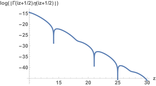
Figure 6: Plot of the logarithm of the absolute vale of $\Gamma\left({iz+\frac{1}{2}}\right)\eta\left({iz+\frac{1}{2}}\right)$ function which is the Baker Akheizer function for the $(\infty,1)$ two matrix model.

9 Obstructions to the Master Matrix for the Two Matrix Model

The fact that the Baker-Akhiezer function for the two matrix model can have complex zeros can lead to an obstruction to the construction of the master matrix for the two matrix model. This is because the master matrix is a special Hermitian matrix whose characteristic polynomial yields the expectation value for the two matrix model in the limit of infinite $N$. That is:

$${\left\langle{\det(b-B}\right\rangle_{N\times N}}=\det(b-{B_{master}})$$ (9.1)

Since $B_{master}$ is Hermitian it’s characteristic polynomial must have real zeros. But we have seen the exact expression for the expectation of the characteristic polynomial in terms of the biorthogonal polynomial $Q_{N}(b)$ which can have complex zeros depending on the potential of the two matrix model. In the large $N$ limit these complex zeros can lead to complex zeros of the Baker-Akhiezer function. The master matrix can never lead to these complex zeros thus we say that there is an obstruction to the construction of the master matrix in those cases.

There are several approaches to construct the master field or master matrix [100] [101] [102] [103] [104] [105] [106] [107] [108] [109] [110] [111] [112]. One has the non-commutative probability algebraic approach of [113]. Here the master matrix take the form of a combination the raising and lowering operators. For example for the $(2,1)$ matrix model the master matrix or operator is $a+{a^{\dagger}}$ with creation and annihilation operators which leads to the representation of the characteristic polynomial in terms of the Hermite polynomials through the relation to the Harmonic oscillator. As discussed above these leads to the Airy function as the Baker-Akhiezer function in the double scaling limit. Notably the zeros of the Baker-Akhiezer function are real which is consistent with the existence of a master matrix in that case. In other cases the polynomials for the two matrix model are not related to a standard quantum mechanical system like the harmonic oscillator. This is especially true for two matrix models whose orthogonal polynomials have complex zeros.

Another approach to the master matrix is the quenched master field [114] [115][116][117] which can be applied to the matrix models discussed in the previous sections. Here one defines the partition function:

$$Z(g)=\int{dAdB{e^{-S(A,B)}}}$$ (9.2)

where $S(A,B)$ is the action of the two matrix model given by:

$$S(A,B)=\frac{1}{g}Tr(V(A+1)-AB)$$ (9.3)

One then introduces a stochastic time $\tau$ and a diagonal matrix $\hat{p}$ as well as stochastic time independent matrices $\hat{a}$ and $\hat{b}$ through:

$$\hat{A}={e^{i\hat{p}\tau}}\hat{a}{e^{-i\hat{p}\tau}}$$

$$\hat{B}={e^{i\hat{p}\tau}}\hat{b}{e^{-i\hat{p}\tau}}$$ (9.4)

The quenched master field equations are then given by:

$$i\left({{{\hat{p}}_{k}}-{{\hat{p}}_{\ell}}}\right){{\hat{a}}_{k\ell}}=-{\left.{\frac{{\delta S}}{{\delta{A_{\ell k}}}}}\right|_{A=\hat{a},B=\hat{b}}}+\hat{\eta}_{k\ell}^{(1)}$$

$$i\left({{{\hat{p}}_{k}}-{{\hat{p}}_{\ell}}}\right){{\hat{b}}_{k\ell}}=-{\left.{\frac{{\delta S}}{{\delta{B_{\ell k}}}}}\right|_{A=\hat{a},B=\hat{b}}}+\hat{\eta}_{k\ell}^{(2)}$$ (9.5)

which reduce to:

$$i\left({{{\hat{p}}_{k}}-{{\hat{p}}_{\ell}}}\right){{\hat{a}}_{k\ell}}=-\frac{1}{g}V^{\prime}(a+I)_{k\ell}+\frac{1}{g}{{\hat{b}}_{k\ell}}+\hat{\eta}_{k\ell}^{(1)}$$

$$i\left({{{\hat{p}}_{k}}-{{\hat{p}}_{\ell}}}\right){{\hat{b}}_{k\ell}}=\frac{1}{g}{{\hat{a}}_{k\ell}}+\hat{\eta}_{k\ell}^{(2)}$$ (9.6)

In these equations $\hat{p}_{i}$ are randomly distributed master momenta and $\hat{\eta}_{k\ell}^{(2)}$ are master noise matrices whose components are Gaussian distributed random numbers. The solution to the quenched master field equations can be formulated as an optimization problem by forming:

$$E_{k\ell}=i\left({{{\hat{p}}_{k}}-{{\hat{p}}_{\ell}}}\right){{\hat{a}}_{k\ell}}+\frac{1}{g}V^{\prime}(a+I)_{k\ell}-\frac{1}{g}{{\hat{b}}_{k\ell}}-\hat{\eta}_{k\ell}^{(1)}$$

$$F_{k\ell}=i\left({{{\hat{p}}_{k}}-{{\hat{p}}_{\ell}}}\right){{\hat{b}}_{k\ell}}-\frac{1}{g}{{\hat{a}}_{k\ell}}-\hat{\eta}_{k\ell}^{(2)}$$ (9.7)

and optimizing:

$$C=\sum\limits_{i,\ell}{\left({E_{i\ell}^{2}+F_{i\ell}^{2}}\right)}$$ (9.8)

Various optimization procedures can be used for finding the minimum of $C$. It is interesting that quantum computing can be used for optimization problems so this is another area of potential application of quantum algorithms to the Riemann hypothesis [118] [119]. If the minimum of $C$ is zero than all the equations are satisfied and the value of $\hat{a}_{k\ell}$ and $\hat{b}_{k\ell}$ determine the Master matrix with real zeros for the expectation value for the characteristic polynomial as $b_{master}$ is Hermitian. If the minimum is not zero than some of the equations could not be satisfied and the master matrix could not be constructed and we say that there is an obstruction. These obstruction could happen if the characteristic polynomial has complex zeros or also if it has real zeros so that an obstruction to the master matrix does not falsify the Riemann hypothesis, but on the other hand if the master matrix can be constructed the the hypothesis would be true.

An alternative to the master matrix equations are the saddle point equations for the two matrix model [120]. The saddle point approach looks at the eigenvalue integral representation of the partition function:

$$Z=\int{\prod\limits_{i=1}^{N}{d{a_{i}}d{b_{i}}\Delta(a)\Delta(b){e^{\frac{1}{g}\sum\limits_{i=1}^{N}{\left({-V({a_{i}}}\right)-{b_{i}}+{a_{i}}{b_{i}})}}}}}$$ (9.9)

with Vandermonde determinants:

$$\Delta(a)=\prod\limits_{i>j}{\left({{a_{i}}-{a_{j}}}\right)}$$

$$\Delta(b)=\prod\limits_{i>j}{\left({{b_{i}}-{b_{j}}}\right)}$$ (9.10)

One then takes the saddle point approximation to the effective potential of the eigenvalues yielding the equations.

$$-\frac{1}{g}V^{\prime}(1+{a_{i}})+\frac{1}{g}{b_{i}}+ \sum\limits_{j\neq i}{\frac{1}{{{a_{i}}-{a_{j}}}}}=0$$

$$\frac{1}{g}{a_{i}}+ \sum\limits_{j\neq i}{\frac{1}{{{b_{i}}-{b_{j}}}}}=0$$ (9.11)

It would be interesting to apply it to the Riemann hypothesis in the two matrix model context as the picture of repelling eigenvalues with supporting numerical data about the Riemann zeros. A description in terms of many fermion ground state wave functions is also possible with the Vandermonde factor being related to a Slater determinant [121] [122] [123]. Finally new approaches based on positivity and the conformal bootstrap would be interesting to apply to the two matrix model approach to the Riemann hypothesis [124] [125] [126] [127].

10 Conclusion

Baker-Akhiezer function	$U(x)$	$z_{3}(N=16)$	$z_{3}$ exact	On CL finite N	infinite N
$Ai(z)$	$i\frac{x^{3}}{3}$	-5.56709	-5.52056	Y	Y
Riemann $\Xi(z)$	$-\log\left(\Phi(x)\right)$	26.5505	25.0109	N	?
Ramanujan $\Xi_{L}(z)$	$-\log\left(\Phi_{L}(x)\right)$	17.6636	17.442777	N	?
$Ai_{(7,1)}(z)$	$\frac{x^{8}}{8}$	7.13834	7.53357	Y	Y
$Ai_{(7,1)}(z,-1,3,0)$	$\frac{x^{8}}{8}+3\frac{x^{4}}{4}-\frac{x^{2}}{2}$	8.50607	8.6996	Y	Y
$Ai_{(7,1)}(z,1,3,3)$	$\frac{x^{8}}{8}+3\frac{x^{6}}{6}+3\frac{x^{4}}{4}+\frac{x^{2}}{2}$	10.5535	10.9217	Y	Y
$K_{iz}(1)$	$\cosh(x)$	5.80583	5.87987	Y	Y
$\Gamma\left({iz+\frac{1}{2}}\right)\eta\left({iz+\frac{1}{2}}\right)$	$\log\left(\frac{e^{-\frac{1}{2}(x+\log(2))}}{\exp\left(e^{-(x+\log(2))}+1\right)}\right)$	26.527	25.0109	N	?

Table 1: Results from studying the Baker-Akhiezer function for $(p,1)$ two matrix models. The third zero of the Baker-Akheizer function was estimated using the polynomial approach for $N=16$ and compared with the exact value. The first two zeros were fixed by a linear transformation. The only Baker-Akhiezer functions we studied with zeros off the critical line (CL) at finite $N$ were the Riemann Xi, Ramanujan L function and the product of gamma and eta functions. Whether these functions have zeros off the critical line as $N$ goes to infinity is unknown and its solution is equivalent to the Riemann and generalized Riemann hypothesis.

In this paper we studied the Riemann Xi function and other functions as Baker-Akhiezer functions for two matrix models. We recorded our results in table 1. For finite $N$ we found zeros off the critical line for the Riemann Xi and Ramanujan L functions using the method of bi-orthogonal polynomials applied to the two matrix model. We studied $N=16$ and it would be interesting to study larger $N$ to see what happens to the zeros off the critical line as $N$ goes to infinity. It would also be interesting to apply other methods to the two matrix model associated with the Riemann Xi function such as the master matrix approach, saddle point method or bootstrap approach. This may give additional information on the fate of the zeros off the critical line at large $N$. Other methods that can be applied include unitary matrix models, phase space and prime factorization applied to the Riemann zeros discussed in [128] [129] [130].

For both the one and two matrix model the characteristic polynomial of the Jacobi matrix yields the the expectation value of the characteristic polynomial which becomes the Baker-Akhiezer function in the large $N$ limit. Unlike the one matrix model, for the two matrix model the Jacobi matrix is not symmetric and for a range of coupling $g$ and deformation parameters $s_{i}$ can develop complex eigenvalues for finite $N$. The important question is what happens to these complex eigenvalues that potentially become zeros off the critical in the scaling limit as $N$ goes to infinity. It is thought that solution to the Riemann hypothesis must in involve the arithmetic properties of the zeta function. The modular invariance properties of the potentials $-\log(\Phi(x))$ and $-\log(\Phi_{L}(x))$ functions may also play a role as these functions can be expressed in terms of theta functions which also have arithmetic properties. Interestingly modular properties of potentials play a role in fundamental physics through modular invariant axion-dilaton potentials [131] [132] [133] [134] [135][136] [137] [138][139] [140] [141]. It would be remarkable (although not unprecedented) if a fundamental problem in mathematics such as the Riemann hypothesis turned out to be related to fundamental problems in the physics of elementary particles.

References

- [1] J.B. Conrey, ”The Reimann Hypothesis”, Notices of AMS (2003).
- [2] W.Konig ”Orthogonal polynomial ensembles in probability theory”, Probability Surveys 2, 385 (2005)
- [3] J.Peca-Medlin, An approach to the Riemann hypothesis through random matrix theory” (2018).
- [4] D.A. Cardon ”matrices related to Dirichlet series”, Journal of Number Theory 130, 27 (2010).
- [5] J.C. Perez-Moure, ”Evidences that the Riemann Hypotheis is true”, (2004).
- [6] Conrey, J. Brian, David W. Farmer, Jon P. Keating, Michael O. Rubinstein, and Nina C. Snaith. ”Integral moments of L-functions.” Proceedings of the London Mathematical Society 91, no. 1 (2005): 33-104.
- [7] M. McGuigan, “Riemann Hypothesis, Matrix/Gravity Correspondence and FZZT Brane Partition Functions,” [arXiv:0708.0645 [math-ph]].
- [8] M. McGuigan, ”Riemann Hypothesis and Master Matrix for FZZT Brane Partition Functions.” arXiv preprint [arXiv:0805.0725 [math-ph] (2008).
- [9] G. Szego, ”Collected papers” (1982).
- [10] Iserles, Arieh, Norsett, Syvert. (1988). On the Theory of Biorthogonal Polynomials. Transactions of The American Mathematical Society - TRANS AMER MATH SOC. 306. 455-455. 10.2307/2000806.
- [11] A. Hashimoto, M. x. Huang, A. Klemm and D. Shih, “Open/closed string duality for topological gravity with matter,” JHEP 05, 007 (2005) doi:10.1088/1126-6708/2005/05/007 [arXiv:hep-th/0501141 [hep-th]].
- [12] J. M. Maldacena, G. W. Moore, N. Seiberg and D. Shih, “Exact vs. semiclassical target space of the minimal string,” JHEP 10, 020 (2004) doi:10.1088/1126-6708/2004/10/020 [arXiv:hep-th/0408039 [hep-th]].
- [13] O. Marchal and M. Cafasso, “Double scaling limits of random matrices and minimal (2m,1) models: The Merging of two cuts in a degenerate case,” J. Stat. Mech. 1104, P04013 (2011) doi:10.1088/1742-5468/2011/04/P04013 [arXiv:1002.3347 [math-ph]].
- [14] C. T. Chan, H. Irie and C. H. Yeh, “Stokes Phenomena and Non-perturbative Completion in the Multi-cut Two-matrix Models,” Nucl. Phys. B 854, 67-132 (2012) doi:10.1016/j.nuclphysb.2011.08.021 [arXiv:1011.5745 [hep-th]].
- [15] C. T. Chan, H. Irie, S. Y. D. Shih and C. H. Yeh, “Macroscopic loop amplitudes in the multi-cut two-matrix models,” Nucl. Phys. B 828, 536-580 (2010) doi:10.1016/j.nuclphysb.2009.10.017 [arXiv:0909.1197 [hep-th]].
- [16] V. A. Kazakov and I. K. Kostov, “Instantons in noncritical strings from the two matrix model,” doi:10.1142/9789812775344_0045 [arXiv:hep-th/0403152 [hep-th]].
- [17] S. M. Carroll, M. E. Ortiz and W. Taylor, “Boundary fields and renormalization group flow in the two matrix model,” Phys. Rev. D 58, 046006 (1998) doi:10.1103/PhysRevD.58.046006 [arXiv:hep-th/9711008 [hep-th]].
- [18] M. Anazawa, A. Ishikawa and H. Itoyama, “Macroscopic three loop amplitudes from the two matrix model,” Phys. Lett. B 362, 59-64 (1995) doi:10.1016/0370-2693(95)01180-X [arXiv:hep-th/9508009 [hep-th]].
- [19] M. Ikehara, “The Continuum limit of the Schwinger-Dyson equations of the one and two matrix model with finite loop length,” Phys. Lett. B 348, 365-376 (1995) doi:10.1016/0370-2693(95)00191-M [arXiv:hep-th/9412120 [hep-th]].
- [20] M. Anazawa, A. Ishikawa and H. Itoyama, “Universal annulus amplitude from the two matrix model,” Phys. Rev. D 52, 6016-6019 (1995) doi:10.1103/PhysRevD.52.6016 [arXiv:hep-th/9410015 [hep-th]].
- [21] J. M. Daul, V. A. Kazakov and I. K. Kostov, “Rational theories of 2-D gravity from the two matrix model,” Nucl. Phys. B 409, 311-338 (1993) doi:10.1016/0550-3213(93)90582-A [arXiv:hep-th/9303093 [hep-th]].
- [22] M. Staudacher, “Combinatorial solution of the two matrix model,” Phys. Lett. B 305, 332-338 (1993) doi:10.1016/0370-2693(93)91063-S [arXiv:hep-th/9301038 [hep-th]].
- [23] J. Alfaro, “The Large N limit of the two Hermitian matrix model by the hidden BRST method,” Phys. Rev. D 47, 4714-4722 (1993) doi:10.1103/PhysRevD.47.4714 [arXiv:hep-th/9207097 [hep-th]].
- [24] M. Marino, R. Schiappa and M. Schwick, “New Instantons for Matrix Models,” [arXiv:2210.13479 [hep-th]].
- [25] D. S. Eniceicu, R. Mahajan, C. Murdia and A. Sen, “Multi-instantons in minimal string theory and in matrix integrals,” JHEP 10, 065 (2022) doi:10.1007/JHEP10(2022)065 [arXiv:2206.13531 [hep-th]].
- [26] J. M. Daul, V. A. Kazakov and I. K. Kostov, “Rational theories of 2-D gravity from the two matrix model,” Nucl. Phys. B 409, 311-338 (1993) doi:10.1016/0550-3213(93)90582-A [arXiv:hep-th/9303093 [hep-th]].
- [27] Brézin, E., Hikami, S. 2000. Characteristic polynomials of random matrices at edge singularities. Physical Review E 62, 3558–3567. doi:10.1103/PhysRevE.62.3558
- [28] J. D. Cohn and S. P. de Alwis, “String field theory for d = 1 matrix models,” Nucl. Phys. B 368, 79-97 (1992) doi:10.1016/0550-3213(92)90198-K
- [29] A. Marshakov, A. Mironov and A. Morozov, “From Virasoro constraints in Kontsevich’s model to W constraints in two matrix model,” Mod. Phys. Lett. A 7, 1345-1360 (1992) doi:10.1142/S0217732392001014 [arXiv:hep-th/9201010 [hep-th]].
- [30] H. Itoyama, “Matrix models at finite N,” [arXiv:hep-th/9111039 [hep-th]].
- [31] P. H. Ginsparg, “Matrix models of 2-d gravity,” [arXiv:hep-th/9112013 [hep-th]].
- [32] G. M. Cicuta, “Matrix models in statistical mechanics and in quantum field theory in the large order limit,” BARI-TH-92-95.
- [33] J. Alfaro, “The Large N limit of the two Hermitian matrix model by the hidden BRST method,” Phys. Rev. D 47, 4714-4722 (1993) doi:10.1103/PhysRevD.47.4714 [arXiv:hep-th/9207097 [hep-th]].
- [34] M. Kaku, “Recent developments in D = 2 string field theory,” Int. J. Mod. Phys. A 9, 3103-3142 (1994) doi:10.1142/S0217751X94001229 [arXiv:hep-th/9403122 [hep-th]].
- [35] L. Bonora and C. S. Xiong, “Two matrix model and c = 1 string theory,” Phys. Lett. B 347, 41-48 (1995) doi:10.1016/0370-2693(95)00153-C [arXiv:hep-th/9405004 [hep-th]].
- [36] H. Aratyn, E. Nissimov, S. Pacheva and A. H. Zimerman, “Two matrix string model as constrained (2+1)-dimensional integrable system,” Phys. Lett. B 341, 19-30 (1994) doi:10.1016/0370-2693(94)01255-5 [arXiv:hep-th/9407017 [hep-th]].
- [37] L. C. de Albuquerque, N. A. Alves and D. Dalmazi, “Yang-Lee zeros of the Ising model on random graphs of nonplanar topology,” Nucl. Phys. B 580, 739-756 (2000) doi:10.1016/S0550-3213(00)00290-X [arXiv:hep-th/9912270 [hep-th]].
- [38] V. A. Kazakov and A. Marshakov, “Complex curve of the two matrix model and its tau function,” J. Phys. A 36, 3107-3136 (2003) doi:10.1088/0305-4470/36/12/315 [arXiv:hep-th/0211236 [hep-th]].
- [39] G. S. Krishnaswami, “Large-N limit as a classical limit: Baryon in two-dimensional QCD and multi-matrix models,” [arXiv:hep-th/0409279 [hep-th]].
- [40] C. T. Chan, H. Irie, S. Y. D. Shih and C. H. Yeh, “Macroscopic loop amplitudes in the multi-cut two-matrix models,” Nucl. Phys. B 828, 536-580 (2010) doi:10.1016/j.nuclphysb.2009.10.017 [arXiv:0909.1197 [hep-th]].
- [41] P. Betzios, U. Gürsoy and O. Papadoulaki, “Matrix Quantum Mechanics on ,” Nucl. Phys. B 928, 356-414 (2018) doi:10.1016/j.nuclphysb.2018.01.019 [arXiv:1612.04792 [hep-th]].
- [42] J. Brunekreef, L. Lionni and J. Thürigen, “One-matrix differential reformulation of two-matrix models,” Rev. Math. Phys. 34, no.08, 2250026 (2022) doi:10.1142/S0129055X2250026X [arXiv:2108.00540 [math-ph]].
- [43] M. L. Mehta, “A Method of Integration Over Matrix Variables,” Commun. Math. Phys. 79, 327-340 (1981) doi:10.1007/BF01208498
- [44] B. Eynard, “The 2-matrix model, biorthogonal polynomials, Riemann-Hilbert problem, and algebraic geometry,” [arXiv:math-ph/0504034 [math-ph]].
- [45] C. T. Chan, H. Irie and C. H. Yeh, “Fractional-Superstring Amplitudes, Multi-Cut Matrix Models and Non-Critical M Theory,” Nucl. Phys. B 838, 75-118 (2010) doi:10.1016/j.nuclphysb.2010.05.007 [arXiv:1003.1626 [hep-th]].
- [46] C. T. Chan, H. Irie and C. H. Yeh, “Stokes Phenomena and Non-perturbative Completion in the Multi-cut Two-matrix Models,” Nucl. Phys. B 854, 67-132 (2012) doi:10.1016/j.nuclphysb.2011.08.021 [arXiv:1011.5745 [hep-th]].
- [47] V. A. Kazakov and A. Marshakov, “Complex curve of the two matrix model and its tau function,” J. Phys. A 36, 3107-3136 (2003) doi:10.1088/0305-4470/36/12/315 [arXiv:hep-th/0211236 [hep-th]].
- [48] S. Y. Alexandrov, V. A. Kazakov and I. K. Kostov, “Time dependent backgrounds of 2-D string theory,” Nucl. Phys. B 640, 119-144 (2002) doi:10.1016/S0550-3213(02)00541-2 [arXiv:hep-th/0205079 [hep-th]].
- [49] A. Chattopadhyay, A. Mitra and H. J. R. van Zyl, “Spread complexity as classical dilaton solutions,” [arXiv:2302.10489 [hep-th]].
- [50] G. Di Ubaldo and G. Policastro, “Ensemble averaging in JT gravity from entanglement in Matrix Quantum Mechanics,” [arXiv:2301.02259 [hep-th]].
- [51] K. Suzuki and T. Takayanagi, “JT gravity limit of Liouville CFT and matrix model,” JHEP 11, 137 (2021) doi:10.1007/JHEP11(2021)137 [arXiv:2108.12096 [hep-th]].
- [52] K. Okuyama and K. Sakai, “FZZT branes in JT gravity and topological gravity,” JHEP 09, 191 (2021) doi:10.1007/JHEP09(2021)191 [arXiv:2108.03876 [hep-th]].
- [53] A. Goel and H. Verlinde, “Towards a String Dual of SYK,” [arXiv:2103.03187 [hep-th]].
- [54] I. Ellwood and A. Hashimoto, “Open/closed duality for FZZT branes in c=1,” JHEP 02, 002 (2006) doi:10.1088/1126-6708/2006/02/002 [arXiv:hep-th/0512217 [hep-th]].
- [55] M.L. Mehta, M. Gaudin, ”On the density of Eigenvalues of a random matrix”, Nuclear Physics, Volume 18, 1960, Pages 420-427, ISSN 0029-5582, doi.org/10.1016/0029-5582(60)90414-4.
- [56] J. M. Daul, V. A. Kazakov and I. K. Kostov, “Rational theories of 2-D gravity from the two matrix model,” Nucl. Phys. B 409, 311-338 (1993) doi:10.1016/0550-3213(93)90582-A [arXiv:hep-th/9303093 [hep-th]].
- [57] T. Tada, “(q,p) critical point from two matrix models,” Phys. Lett. B 259, 442-447 (1991) doi:10.1016/0370-2693(91)91654-E
- [58] H. Itoyama, “Matrix models at finite N,” [arXiv:hep-th/9111039 [hep-th]].
- [59] T. Tada and M. Yamaguchi, “P and Q operator analysis for two matrix model,” Phys. Lett. B 250, 38-43 (1990) doi:10.1016/0370-2693(90)91151-Z
- [60] M. Fukuma and H. Irie, “A String field theoretical description of (p,q) minimal superstrings,” JHEP 01, 037 (2007) doi:10.1088/1126-6708/2007/01/037 [arXiv:hep-th/0611045 [hep-th]].
- [61] L. Bonora, “Two matrix models, W algebras and 2-D gravity,” SISSA-170-94-EP.
- [62] M. R. Douglas, “The Two matrix model,”
- [63] T. Banks, “Matrix models, string field theory and topology,” RU-90-52.
- [64] B. Eynard, “Large random matrices: Eigenvalue distribution,” [arXiv:hep-th/9401165 [hep-th]].
- [65] B. Eynard, “Large N expansion of the 2 matrix model,” JHEP 01, 051 (2003) doi:10.1088/1126-6708/2003/01/051 [arXiv:hep-th/0210047 [hep-th]].
- [66] M. Bertola, B. Eynard and J. Harnad, “Differential systems for biorthogonal polynomials appearing in 2-matrix models and the associated Riemann-Hilbert problem,” Commun. Math. Phys. 243, 193-240 (2003) doi:10.1007/s00220-003-0934-1 [arXiv:nlin/0208002 [nlin.SI]].
- [67] M. Bertola, B. Eynard and J. Harnad, “Duality of spectral curves arising in two matrix models,” Theor. Math. Phys. 134, 27-38 (2003) doi:10.1023/A:1021811505196 [arXiv:nlin/0112006 [nlin.SI]].
- [68] M. Bertola, B. Eynard and J. P. Harnad, “Duality, biorthogonal polynomials and multimatrix models,” Commun. Math. Phys. 229, 73-120 (2002) doi:10.1007/s002200200663 [arXiv:nlin/0108049 [nlin.SI]].
- [69] M. Bertola and B. Eynard, “Mixed correlation functions of the two matrix model,” J. Phys. A 36, 7733-7750 (2003) doi:10.1088/0305-4470/36/28/304 [arXiv:hep-th/0303161 [hep-th]].
- [70] M. Bertola, “Free energy of the two matrix model / dToda tau function,” Nucl. Phys. B 669, 435-461 (2003) doi:10.1016/j.nuclphysb.2003.07.029 [arXiv:hep-th/0306184 [hep-th]].
- [71] M. Bertola, “Second and third order observables of the two matrix model,” JHEP 11, 062 (2003) doi:10.1088/1126-6708/2003/11/062 [arXiv:hep-th/0309192 [hep-th]].
- [72] M. Bertola, B. Eynard and J. Harnad, “Semiclassical orthogonal polynomials, matrix models and isomonodromic tau functions,” Commun. Math. Phys. 263, 401-437 (2006) doi:10.1007/s00220-005-1505-4 [arXiv:nlin/0410043 [nlin.SI]].
- [73] B. Eynard, “Loop equations for the semiclassical 2-matrix model with hard edges,” J. Stat. Mech. 0510, P10006 (2005) doi:10.1088/1742-5468/2005/10/P10006 [arXiv:math-ph/0504002 [math-ph]].
- [74] J. Ambjorn, J. Jurkiewicz, R. Loll and G. Vernizzi, “Lorentzian 3-D gravity with wormholes via matrix models,” JHEP 09, 022 (2001) doi:10.1088/1126-6708/2001/09/022 [arXiv:hep-th/0106082 [hep-th]].
- [75] R. d. Koch, A. Jevicki, X. Liu, K. Mathaba and J. P. Rodrigues, “Large N optimization for multi-matrix systems,” JHEP 01, 168 (2022) doi:10.1007/JHEP01(2022)168 [arXiv:2108.08803 [hep-th]].
- [76] X. Han and S. A. Hartnoll, “Deep Quantum Geometry of Matrices,” Phys. Rev. X 10, no.1, 011069 (2020) doi:10.1103/PhysRevX.10.011069 [arXiv:1906.08781 [hep-th]].
- [77] E. Rinaldi, X. Han, M. Hassan, Y. Feng, F. Nori, M. McGuigan and M. Hanada, “Matrix-Model Simulations Using Quantum Computing, Deep Learning, and Lattice Monte Carlo,” PRX Quantum 3, no.1, 010324 (2022) doi:10.1103/PRXQuantum.3.010324 [arXiv:2108.02942 [quant-ph]].
- [78] Brunekreef, Joren, Luca Lionni, and Johannes Thürigen. ”One-matrix differential reformulation of two-matrix models.” arXiv preprint arXiv:2108.00540 (2021).
- [79] Hernández-del-Valle, G. 2015. ”On the zeros of the Pearcey integral and a Rayleigh-type equation,” arXiv e-prints. doi:10.48550/arXiv.1506.02502
- [80] Duits, M., Kuijlaars, A. B. J., Mo, M. Y. 2010. The Hermitian two matrix model with an even quartic potential. arXiv e-prints. doi:10.48550/arXiv.1010.4282
- [81] Duits, M., Kuijlaars, A. B. J., Mo, M. Y. 2012. Asymptotic analysis of the two matrix model with a quartic potential. arXiv e-prints. doi:10.48550/arXiv.1210.0097
- [82] Universality in the Two Matrix Model with a Monomial Quartic and a General Even Polynomial Potential. Communications in Mathematical Physics 291, 863–894. doi:10.1007/s00220-009-0893-2
- [83] Duits, M., Kuijlaars, A. B. J. 2008. Universality in the two matrix model: a Riemann-Hilbert steepest descent analysis. arXiv e-prints. doi:10.48550/arXiv.0807.4814
- [84] Duits, M. 2013. Painlevé kernels in Hermitian matrix models. arXiv e-prints. doi:10.48550/arXiv.1302.1710
- [85] Richard Bruce Paris. 2012. “On the Asymptotics and Zeros of a Class of Fourier Integrals”. European Journal of Pure and Applied Mathematics 5 (3):260-81.
- [86] N G de Bruijn. The roots of trigonometric integrals, Duke Math. J. 17:197–226, 1950.
- [87] D. Senouf, ”Asymptotic and numerical approximations of the zeros of Fourier transforms”, SIAM J. Analysis 27, 1102 (1996).
- [88] D A Cardon. Fourier transforms having only real zeros, Proc. Amer. Math. Soc. 133:1349–1356, 2004.
- [89] J Kamimoto, H Ki and Y-O Kim. On the multiplicities of the zeros of Laguerre–Pólya functions, Proc. Amer. Math. Soc. 128:189–194, 1999.
- [90] G.Polya, ”On the zeros of an integral function represented by Fourier’s integral”, Messenger of Math 52, 185 (1923).
- [91] Breuer, J., Duits, M. 2013. The Nevai condition and a local law of large numbers for orthogonal polynomial ensembles. arXiv e-prints. doi:10.48550/arXiv.1301.2061
- [92] Dominici, D., ”Asymptotic analysis of the Hermite polynomials from their differential-difference equation.” arXiv Mathematics e-prints. doi:10.48550/arXiv.math/0601078
- [93] H. Ki, ”The zeros of Fourier Transformations”.
- [94] D.Dimitrov ,P. Rusev (2011). Zeros of entire Fourier transforms. East Journal on Approximations. 17.
- [95] G.Franca, A. LeClair, A. 2013. On the zeros of L-functions. arXiv e-prints. doi:10.48550/arXiv.1309.7019
- [96] Cardon, David A. and Sharleen A. Roberts. “An equivalence for the Riemann Hypothesis in terms of orthogonal polynomials.” J. Approx. Theory 138 (2006): 54-64.
- [97] Mazhouda, Kamel and Sami Omar. “The Cardon and Robert Criterion for the Riemann hypothesis.” Analysis 33 (2013): 309 - 318.
- [98] Newman, Charles M., and Wei Wu. ”Constants of de Bruijn-Newman type in analytic number theory and statistical physics.” arXiv preprint arXiv:1901.06596 (2019).
- [99] R. Mahajan, D. Stanford and C. Yan, “Sphere and disk partition functions in Liouville and in matrix integrals,” JHEP 07, 132 (2022) doi:10.1007/JHEP07(2022)132 [arXiv:2107.01172 [hep-th]].
- [100] E. Witten, “THE 1 / N EXPANSION IN ATOMIC AND PARTICLE PHYSICS,” NATO Sci. Ser. B 59, 403-419 (1980) doi:10.1007/978-1-4684-7571-5_21
- [101] S. Coleman, “Aspects of Symmetry: Selected Erice Lectures,” Cambridge University Press, 1985, ISBN 978-0-521-31827-3 doi:10.1017/CBO9780511565045
- [102] G. ’t Hooft, “A Planar Diagram Theory for Strong Interactions,” Nucl. Phys. B 72, 461 (1974) doi:10.1016/0550-3213(74)90154-0
- [103] J. Carlson, J. Greensite, M. B. Halpern and T. Sterling, “DETECTION OF MASTER FIELDS NEAR FACTORIZATION,” Nucl. Phys. B 217, 461-464 (1983) doi:10.1016/0550-3213(83)90157-8
- [104] M. B. Halpern, “MICROCANONICAL MASTER FIELDS,” Nucl. Phys. B 254, 603-618 (1985) doi:10.1016/0550-3213(85)90237-8
- [105] M. B. Halpern and C. Schwartz, “Infinite dimensional free algebra and the forms of the master field,” Int. J. Mod. Phys. A 14, 4653-4686 (1999) doi:10.1142/S0217751X99002189 [arXiv:hep-th/9903131 [hep-th]].
- [106] O. Haan, “LARGE N AS A THERMODYNAMIC LIMIT,” Phys. Lett. B 106, 207-210 (1981) doi:10.1016/0370-2693(81)90909-6
- [107] R. Gopakumar, “N = 1 theories and a geometric master field,” JHEP 05, 033 (2003) doi:10.1088/1126-6708/2003/05/033 [arXiv:hep-th/0211100 [hep-th]].
- [108] O. Haan, “On the Structure of Planar Field Theory,” Z. Phys. C 6, 345 (1980) doi:10.1007/BF01474809
- [109] L. Accardi, I. Y. Aref’eva, S. V. Kozyrev and I. V. Volovich, “The Master field for large N matrix models and quantum groups,” Mod. Phys. Lett. A 10, 2323-2334 (1995) doi:10.1142/S0217732395002489 [arXiv:hep-th/9503041 [hep-th]].
- [110] M. Engelhardt and S. Levit, “Variational master field for large N interacting matrix models: Free random variables on trial,” Nucl. Phys. B 488, 735-774 (1997) doi:10.1016/S0550-3213(97)00043-6 [arXiv:hep-th/9609216 [hep-th]].
- [111] T. Kuroki, “Master field on fuzzy sphere,” Nucl. Phys. B 543, 466-484 (1999) doi:10.1016/S0550-3213(98)00815-3 [arXiv:hep-th/9804041 [hep-th]].
- [112] M. R. Douglas, “Stochastic master fields,” Phys. Lett. B 344, 117-126 (1995) doi:10.1016/0370-2693(94)01547-P [arXiv:hep-th/9411025 [hep-th]].
- [113] R. Gopakumar and D. J. Gross, “Mastering the master field,” Nucl. Phys. B 451, 379-415 (1995) doi:10.1016/0550-3213(95)00340-X [arXiv:hep-th/9411021 [hep-th]].
- [114] J. Greensite and M. B. Halpern, “QUENCHED MASTER FIELDS,” Nucl. Phys. B 211, 343 (1983) doi:10.1016/0550-3213(83)90413-3
- [115] J. Greensite, “Variational Method for Quenched Master Fields,” Phys. Lett. B 121, 169-172 (1983) doi:10.1016/0370-2693(83)90908-5
- [116] J. M. Alberty and J. Greensite, “APPROXIMATION TECHNIQUES FOR THE QUENCHED MASTER FIELD EQUATIONS,” Nucl. Phys. B 238, 39-60 (1984) doi:10.1016/0550-3213(84)90465-6
- [117] F. R. Klinkhamer, “A first look at the bosonic master-field equation of the IIB matrix model,” Int. J. Mod. Phys. D 30, no.13, 2150105 (2021) doi:10.1142/S0218271821501054 [arXiv:2105.05831 [hep-th]].
- [118] M. McGuigan, “Quantum Computing and the Riemann Hypothesis,” [arXiv:2303.04602 [quant-ph]].
- [119] W. van Dam, Wim. ”Quantum computing and zeroes of zeta functions.” arXiv preprint quant-ph/0405081 (2004).
- [120] V. A. Kazakov, “Solvable matrix models,” [arXiv:hep-th/0003064 [hep-th]].
- [121] D. J. E. Callaway, “Random matrices, fractional statistics and the quantum Hall effect,” Phys. Rev. B 43, 8641 (1991) doi:10.1103/PhysRevB.43.8641
- [122] A. Cappelli, C. A. Trugenberger and G. R. Zemba, “Large N limit in the quantum Hall Effect,” Phys. Lett. B 306, 100-107 (1993) doi:10.1016/0370-2693(93)91144-C [arXiv:hep-th/9303030 [hep-th]].
- [123] A. Cappelli and M. Riccardi, “Matrix model description of Laughlin Hall states,” J. Stat. Mech. 0505, P05001 (2005) doi:10.1088/1742-5468/2005/05/P05001 [arXiv:hep-th/0410151 [hep-th]].
- [124] V. Kazakov and Z. Zheng, “Analytic and numerical bootstrap for one-matrix model and “unsolvable” two-matrix model,” JHEP 06, 030 (2022) doi:10.1007/JHEP06(2022)030 [arXiv:2108.04830 [hep-th]].
- [125] H. W. Lin, “Bootstrap bounds on D0-brane quantum mechanics,” [arXiv:2302.04416 [hep-th]].
- [126] H. W. Lin, “Bootstraps to strings: solving random matrix models with positivity,” JHEP 06, 090 (2020) doi:10.1007/JHEP06(2020)090 [arXiv:2002.08387 [hep-th]].
- [127] X. Han, S. A. Hartnoll and J. Kruthoff, “Bootstrapping Matrix Quantum Mechanics,” Phys. Rev. Lett. 125, no.4, 041601 (2020) doi:10.1103/PhysRevLett.125.041601 [arXiv:2004.10212 [hep-th]].
- [128] P. Dutta and S. Dutta, “Phase Space Distribution of Riemann Zeros,” J. Math. Phys. 58, no.5, 053504 (2017) doi:10.1063/1.4982737 [arXiv:1610.07743 [hep-th]].
- [129] A. Chattopadhyay, P. Dutta and S. Dutta, “Emergent Phase Space Description of Unitary Matrix Model,” JHEP 11, 186 (2017) doi:10.1007/JHEP11(2017)186 [arXiv:1708.03298 [hep-th]].
- [130] A. Chattopadhyay, P. Dutta, S. Dutta and D. Ghoshal, “Matrix Model for Riemann Zeta via its Local Factors,” Nucl. Phys. B 954, 114996 (2020) doi:10.1016/j.nuclphysb.2020.114996 [arXiv:1807.07342 [math-ph]].
- [131] M. Cvetic and A. A. Tseytlin, “Charged string solutions with dilaton and modulus fields,” Nucl. Phys. B 416, 137-172 (1994) doi:10.1016/0550-3213(94)90581-9 [arXiv:hep-th/9307123 [hep-th]].
- [132] J. Garcia-Bellido and M. Quiros, “String effective actions and cosmological stability of scalar potentials,” Nucl. Phys. B 385, 558-570 (1992) doi:10.1016/0550-3213(92)90058-J [arXiv:hep-th/9204079 [hep-th]].
- [133] J. H. Horne and G. W. Moore, “Chaotic coupling constants,” Nucl. Phys. B 432, 109-126 (1994) doi:10.1016/0550-3213(94)90595-9 [arXiv:hep-th/9403058 [hep-th]].
- [134] E. Gonzalo, L. E. Ibáñez and Á. M. Uranga, “Modular symmetries and the swampland conjectures,” JHEP 05, 105 (2019) doi:10.1007/JHEP05(2019)105 [arXiv:1812.06520 [hep-th]].
- [135] A. Font, L. E. Ibanez, D. Lust and F. Quevedo, “Strong - weak coupling duality and nonperturbative effects in string theory,” Phys. Lett. B 249, 35-43 (1990) doi:10.1016/0370-2693(90)90523-9
- [136] N. Gendler, M. Kim, L. McAllister, J. Moritz and M. Stillman, “Superpotentials from singular divisors,” JHEP 11, 142 (2022) doi:10.1007/JHEP11(2022)142 [arXiv:2204.06566 [hep-th]].
- [137] R. Donagi, A. Grassi and E. Witten, “A Nonperturbative superpotential with E(8) symmetry,” Mod. Phys. Lett. A 11, 2199-2212 (1996) doi:10.1142/S0217732396002198 [arXiv:hep-th/9607091 [hep-th]].
- [138] G. Curio and D. Lust, “A Class of N=1 dual string pairs and its modular superpotential,” Int. J. Mod. Phys. A 12, 5847-5866 (1997) doi:10.1142/S0217751X97003066 [arXiv:hep-th/9703007 [hep-th]].
- [139] J. M. Leedom, N. Righi and A. Westphal, “Heterotic de Sitter beyond modular symmetry,” JHEP 02, 209 (2023) doi:10.1007/JHEP02(2023)209 [arXiv:2212.03876 [hep-th]].
- [140] S. Alexander, K. Dasgupta, A. Maji, P. Ramadevi and R. Tatar, “de Sitter State in Heterotic String Theory,” [arXiv:2303.12843 [hep-th]].
- [141] N. Cribiori and D. Lust, “A note on modular invariant species scale and potentials,” [arXiv:2306.08673 [hep-th]].