RSRM: Reinforcement Symbolic Regression Machine

Abstract

In nature, the behaviors of many complex systems can be described by parsimonious math equations. Automatically distilling these equations from limited data is cast as a symbolic regression process which hitherto remains a grand challenge. Keen efforts in recent years have been placed on tackling this issue and demonstrated success in symbolic regression. However, there still exist bottlenecks that current methods struggle to break when the discrete search space tends toward infinity and especially when the underlying math formula is intricate. To this end, we propose a novel Reinforcement Symbolic Regression Machine (RSRM) that masters the capability of uncovering complex math equations from only scarce data. The RSRM model is composed of three key modules: (1) a Monte Carlo tree search (MCTS) agent that explores optimal math expression trees consisting of pre-defined math operators and variables, (2) a Double Q-learning block that helps reduce the feasible search space of MCTS via properly understanding the distribution of reward, and (3) a modulated sub-tree discovery block that heuristically learns and defines new math operators to improve representation ability of math expression trees. Biding of these modules yields the state-of-the-art performance of RSRM in symbolic regression as demonstrated by multiple sets of benchmark examples. The RSRM model shows clear superiority over several representative baseline models.

1 Introduction

The pursuit of mathematical expressions through data represents a crucial undertaking in contemporary scientific research. The availability of quantitative mathematical expressions to depict natural relationships enhances human comprehension and yields more precise insights. Parsing solutions offer superior interpretability and generalization compared to numerical solutions generated by neural networks. Additionally, simple expressions exhibit computational efficiency advantages over the latter. Consequently, these techniques have found applications in various fields, including physics [1, 2, 3] and material sciences [4], in recent years.

The initial process of fitting expressions involves polynomial interpolation to derive an equation, followed by the application of the SINDy method [5] utilizing sparse regression to identify appropriate mathematical expressions based on predefined library of candidate terms. These methods effectively reduce the search space from an infinitely large set of possibilities to a limited fixed set of expressions, thereby narrowing down the search process [6, 7, 8]. However, the applicability of this approach is limited, since the compositional structure of many equations cannot be predefined in advance. Therefore, there is a need for more comprehensive methods to search for expressions.

The EQL (Equation Learner) [9, 10] model was then introduced as a novel method in symbolic learning. The EQL model addressed the limitations of traditional activation functions used in deep neural networks, by incorporating symbolic operators as activation functions. This modification enabled the neural network to generate more complex functional relationships, allowing for the discovery of intricate math expressions. However, given its compact structure of EQL, optimizing the sparse network to distill parsimonious equation becomes a key challenge.

Another approach involves generating optimal expression trees [11], where internal nodes correspond to operators and each leaf node represents a constant or variable. By recursively computing the expressions of the sub-trees, these expression trees can be transformed into the original math expressions. Initially, genetic programming (GP) [12, 13, 14] were employed to address these problems. Although GP showed promise, its sensitivity to parameter settings leads to instability. Deep learning methods emerged then to tackle the problem. SymbolicGPT [15] utilizes a generative model like GPT to create expression trees, while while AIFeynman [1] uses neural networks to analyze the relationships and dependencies between variables and search for relevant expressions. An updated version of AIFeynman [16] has been developed, offering faster and more precise expression search capabilities. Additionally, reinforcement learning approaches [3] have been introduced, which utilizes the Monte Carlo tree search method to explore and discover expressions, along with a module-transplant module that generates new expressions based on existing ones. Deep reinforcement learning methods, e.g. DSR [17], utilize recurrent neural networks to learn expression features and generate probabilities. A search algorithm samples these probabilities to generate a batch of expressions, which are subsequently evaluated for performance. The network is then trained using these evaluations. Combining DSR and GP leads to a new model called NGGP [18] achieved better performance. Additionally, pre-trained generative models [19] and end-to-end transformer modules [20, 21] have been also employed to achieve improved expression search results.

Nevertheless, the existing methods still struggle with generating lengthy and complex equations, and are faced with issues related to overfitting. To overcome these challenges, we propose a model named Reinforcement Symbolic Regression Machine (RSRM) that masters the capability of uncovering complex math equations from only scarce data. The search strategy in our model is based on the synergy between double Q-learning [22] and Monte Carlo tree search [23]. By employing two reinforcement methods without deep learning, we aim to mitigate overfitting concerns. To capture the distribution of equations, we utilize double Q-learning, while Monte Carlo Tree Search (MCTS) aids in generating new expressions. Additionally, to address the challenge of lengthy and hard equations, we introduce an interpolation method to identify whether the equation exhibits symmetry prior to each search, followed by a modulated sub-tree discovery block. If symmetry is present, we pre-process the equation accordingly to simplify the subsequent search process. This approach effectively reduces the difficulty associated with specific equations. The sub-tree form-discovery module is proposed to examine whether the few expressions that perform well adhere to a specific form. For instance, if both $e^{x}-x$ and $e^{x}+x$ yield favorable results, the expression can be confirmed as $e^{x}+f(x)$, thereby allowing us to focus on finding $f(x)$. This divide-and-conquer algorithm enables a step-by-step search for equations, facilitating the generation of long expressions.

The main contributions of this paper are presented as follows. Our proposed RSRM model offers a novel solution to the search for mathematical expressions. By incorporating double Q-learning and Monte Carlo tree search, we effectively address issues of overfitting and generate new expressions. Through the utilization of modulated sub-tree discovery block, we handle equations with symmetry, reducing their complexity. Furthermore, the block also assists in dealing with long equations by identifying common patterns. By following this comprehensive approach, we enhance the efficiency and effectiveness of the expression search process. As a result of these advancements, the RSRM model demonstrates clear superiority over several representative baseline models. Its state-of-the-art performance surpasses that of the baseline models in terms of accuracy and generalization ability.

2 Background

Genetic Programming: Genetic programming [24, 25, 12] is employed to iteratively improve expression trees in order to approximate the optimal expression tree. The mutation step in GP enables random mutations in the expression tree, while genetic recombination allows for the exchange of sub-trees between expression trees, leading to the creation of new expression trees based on the knowledge acquired from previous generations. This “genetic evolution” process progressively yields highly favorable outcomes after a few generations.

Double Q-Learning: Double Q-learning [22] is a variant of Q-learning that employs two separate Q-value functions. During training, one structure’s results are used to train the other structure with a random 50% probability. During decision-making, both models collaborate to make decisions. This approach mitigates overestimation issues by ensuring that Q-value updates are not solely based on values used for action selection. As a result, more accurate Q-value estimation is achieved, leading to improved agent performance.

Monte Carlo Tree Search: MCTS [23] is a decision-making search algorithm that constructs a search tree representing possible game states and associated values. It employs stochastic simulations to explore the tree and determine the value of each node. This algorithm gained prominence via its adoption by the AlphaZero team [26]. MCTS consists of four steps in each iteration: (1) selection, (2) expansion, (3) simulation, and (4) backpropagation. During selection, the best child node is chosen based on certain criteria. If an expandable node lacks children, it is extended by adding available children. The simulation step involves simulating the current state before selecting the next node, often using the Upper Confidence Bound for Trees (UCT) algorithm to calculate the selection probabilities. Finally, in the backpropagation step, the reward function evaluates child nodes, and their values are used to update the values of parent nodes in the tree.

$$UCT(n)=\bar{Q}(v^{\prime})+c\sqrt{\frac{\ln(N(v))}{N(v^{\prime})}}.$$ (1)

Here, $\bar{Q}(v^{\prime})$ means the average reward of child node, $N(v)$ and $N(v^{\prime})$ means the visit time of node and its child. The first part makes the nodes with high expectations visit more often, and the second part ensures that the nodes with fewer visits have a higher probability of being selected.

3 Method

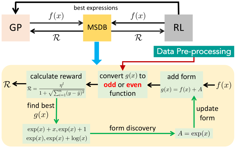
Figure 1: The proposed RSRM utilizes a schematic flow comprising several steps. First, the function is put into the data pre-processing module to determine the parity, followed by a RL-guided search in the Modulated Sub-tree Discovery Block (MSDB) to manipulate expressions and evaluate their form. The discovered equations are then refined using GP. MSDB is continuously updated based on the identified equations.

The proposed RSRM model consists of a three-step symbolic learning process: reinforcement learning-based expression search, GP tuning, and modulated expression form discovery. Through these steps, our model effectively learns and represents the relationship present in the data, facilitating accurate and interpretable modeling. The schematic representation of RSRM is depicted in Figure 1. Full settings of our model are in Appendix A.

3.1 Expression Tree

In the context of symbolic learning tasks, the underlying objective is to transform the given task into the generation of an optimal expression tree [11], which represents a mathematical expression. The expression tree consists of internal nodes that correspond to operators (e.g., $+,-,\times,\div,\log,\exp,\sin,\cos$) and leaf nodes that correspond to constants (e.g., $1,2$) or variables (e.g., $x$). By recursively computing the expressions of the sub-trees, the expression tree can be transformed into the original mathematical expressions. The process of generating an expression tree follows a recursive method where operators are added until no more can be added. This approach simplifies the task of creating expressions as it focuses on constructing the expression tree, which can be easily generated using recursive techniques. By adopting the concept of expression trees, symbolic learning tasks can be effectively addressed by generating and manipulating these trees, enabling the representation and computation of complex mathematical expressions.

In contrast to previous methods, we employ a hierarchical traversal strategy for generating expression trees. This is motivated by the Monte Carlo tree search algorithm, where conducting more searches on vertices that are filled earlier is deemed more beneficial. In the context of constructing expression trees, this implies that higher-level nodes in the tree carry greater significance. Consequently, we adopt a layer-by-layer search method, ensuring that higher-level regions of the tree receive a higher number of search iterations. By prioritizing the traversal of higher-level nodes, we place emphasis on exploring and refining the more influential components of the expression tree. This hierarchical approach allows us to effectively capture and exploit the hierarchical structure of the problem, potentially leading to improved performance and more meaningful results.

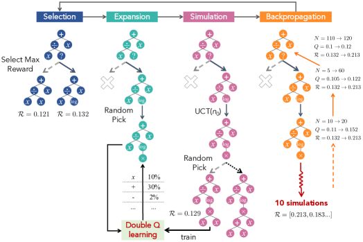
Figure 2: Schematic of the proposed RL search. MCTS selects functions based on the maximum reward, expands them using the results of Q-learning, simulates node selection through the UCT function, randomly fills the current tree, and provides rewards to double Q-learning. Once the generation is complete, the rewards are back-propagated to the parent node.

3.2 Reinforcement Learning Guided Search

The search step relies on the double Q-learning and MCTS algorithms, which are shown in Figure 2. The specific algorithm is shown in Algorithm 1.

Reward function: The reward function used in our approach is based on the root mean square error (RMSE) and is designed to evaluate the fit of the generated equations to the measured data. It promotes concise and accurate expressions by assigning higher rewards to shorter and more precise functions. The reward function is computed as follows:

$$\mathcal{R}=\frac{\eta^{l}}{1+\sqrt{\sum_{i=1}^{n}(y_{i}-\hat{y_{i}})^{2}}},$$ (2)

where $\eta$ denotes a discount factor that promotes concise results, $l$ the number of nodes in the expression tree, and $y_{i}$ and $\hat{y_{i}}$ the true value and the predicted value generated by the MSDB with the output of Reinforcement Learning Search of the $i$th data point, respectively. By using this reward function, our approach encourages the discovery of equations that minimize the RMSE and favors shorter and more concise expressions, leading to higher reward values for functions that provide better fits to the data.

Algorithm 1 Expression generation by RSRM

dataset $\mathcal{S}_{data}$, current expression form $\mathcal{F}$

discount rate $\eta$, training rounds $t_{r}$, UCT const $c$, minimum selected times $n_{0}$

best expression

Initiate $S$ as top of MTCS

Selection:

$a\leftarrow$ children of $S$ with maxium $\mathcal{R}$ $\triangleright$ Greedy selection

$S$ take action $a$

Simulation:

$S^{\prime}\leftarrow S$

repeat

     if children of $S$ is empty then Expand $S^{\prime}$

     end if

     if $\exists x\in$ children of $S^{\prime}\rightarrow(N(x)<n_{0})$ then $a^{\prime}\leftarrow x$ $\triangleright$ Select child with visit times < $n_{0}$

     else $a^{\prime}\leftarrow$ randomly choose child of $S^{\prime}$ by $UCT$ $\triangleright$ Select through UCT function

     end if

     $S^{\prime}$ take action $a^{\prime}$, $S^{\prime\prime}\leftarrow S^{\prime}$, Fill up randomly $S^{\prime\prime}$

     double Q-learning $\leftarrow S^{\prime},a^{\prime},\mathcal{R}$ of $S^{\prime\prime}$ $\triangleright$ train double Q-learning by simulated reward

until $S^{\prime}$ is full

Expansion

children of $S\rightarrow$ double Q-learning $\rightarrow p_{children}$ $\triangleright$ estimate initial possibility of each child

Back-propagate $\mathcal{R}$ of $S^{\prime}$ based on $\mathcal{F}$

Greedy selection: Our method employs greedy selection, similar to SPL [3]. Instead of selecting the token with the highest UCT (Eq. 1) score, we choose the token that currently yields the best reward (Eq. 2). This ensures the selection of tokens leading to expressions resembling the current best one, potentially resulting in improved expressions.

Simulated reward: At each token generation, the entire expression tree is randomly completed based on the current tree. The reward is then computed using the reward function and fed back to double Q-learning for training. This approach avoids excessive rounds of learning at the top node and filters out irrelevant nodes initially.

Parameter optimization: Parameter placeholders are used in expressions, treating each parameter as an unknown variable. Real variables are substituted into the original equation, and the parameters are optimized to minimize the error between predicted value and real value. The BFGS [27] algorithm, available in the scipy [28] module in Python, is used for optimization. Gaussian random numbers with unit mean and variance serve as better starting points for optimization.

3.3 Modulated Sub-tree Discovery

Our approach incorporates three specific search forms to enhance the exploration and analysis of equations, where $\mathcal{A}$ represents a fixed form and $f(x)$ represents a learnable part. The three forms are explained as follows:

• $\mathcal{A}\pm f(x)$: This search form focuses on identifying expressions of the form like $e^{x}-x$ and $e^{x}+x$. By recognizing this pattern, we can effectively explore and analyze equations that follow the structure of $e^{x}\pm f(x)$.

• $\mathcal{A}\times f(x)$: In this search form, we target expressions such as $1.57e^{x}$ and $1.56e^{x}+x$, aiming to detect equations of the form $e^{x}\times f(x)$.

• $\mathcal{A}^{f(x)}$: The search form $\mathcal{A}^{f(x)}$ is designed to recognize equations like $(e^{x})^{2.5}$ and $(e^{x})^{e}$, indicating the presence of expressions in the form $(e^{x})^{f(x)}$.

The complete from-discovery algorithm, which outlines the procedure for selecting and generating the search form among the three options, is provided in Algorithm 2.

Algorithm 2 Search for the form of the expression through the generated expressions

symbol set $\mathcal{S}_{sym}$, best expression set $\mathcal{S}_{best}$

discount rate $\eta$, selection ratio $k_{s}$, expression percentage ratio $k_{p}$, maximum select number $N$

the form of the expression $\mathcal{F}$

$l\leftarrow$ length of $(\mathcal{S}_{best})$

Sort $\mathcal{S}_{best}$ by $\mathcal{R}$ decent

for $i$ in $1,2...l$  do

     if $i\leq N$ and $\mathcal{R}(\mathcal{S}_{best}[i])\geq k\times\mathcal{R}_{max}$ then $\triangleright$ If number of $\mathcal{G}$ exceeds or $\mathcal{R}$ is low, break out

         $\mathcal{D}=\mathcal{D}+\text{Split}(\mathcal{S}_{best}[i])$ $\triangleright$ Occurrences of function in Split-by-addition($\mathcal{S}_{best}[i]$) $+1$

     end if

end for

$\mathcal{G}_{0}\leftarrow\mathcal{D}$ with maximum number of occurrences.

if $\exists\mathcal{C}\notin Z\rightarrow\mathcal{G}_{0}=\mathcal{A}^{\mathcal{C}}$ then $\mathcal{F}=\mathcal{A}^{f(x)}$$\triangleright$ The form is $\mathcal{A}^{f(x)}$

else if $\exists\mathcal{C}\notin Z\rightarrow\mathcal{G}_{0}=\mathcal{A}\times\mathcal{C}$ then $\mathcal{F}=\mathcal{A}\times f(x)$$\triangleright$ The form is $\mathcal{A}\times f(x)$

else

     $\mathcal{F}=f(x)$$\triangleright$ The form is $\mathcal{A}\pm F(x)$

     for $\mathcal{G}$ in $\mathcal{D}$ do

         if Occurrences of $\mathcal{G}\geq l\times k_{p}$ then $\mathcal{F}=\mathcal{F}+\mathcal{G}$$\triangleright$ Add $\mathcal{G}$ to $\mathcal{A}$

         end if

     end for

end if

Splitting by Addition: In this step, we perform the following process: Convert the formula, which is represented as a token set, into a string expression using a library like sympy [29]. Expand the expression into a sum of simpler expressions. Split the expanded expression into multiple simple expressions using sum or difference notation. Store these simple expressions in a dictionary for subsequent analysis and computation, while also keeping track of the count for each simple expression. This process allows us to break down the formula into its constituent parts, making it easier to work with and analyze individual expressions separately.

These search forms enable our approach to classify equations into different structural patterns, facilitating more focused and efficient exploration. By incorporating RL or GP techniques with the MSDB, we can dynamically modify the $f(x)$ part in each search form and generate equations $g(x)$ that conform to the identified patterns.

We then introduce a data pre-processing module determine the potential parity of the underlying equation. The cubic spline [30] is applied for equation fitting, generating a function. Subsequently, this function is utilized to compute the relationship between $y(-x)$ and $y(x)$, enabling determination of whether $y(x)$ is an odd, even, or neither function, where $y(x)$ means the relation of $x$ and $y$ in given data.

When the error between $y(-x)$ and $y(x)$ remains below $E_{sym}$, the function is considered even with respect to $x$. Negative values of the independent variables are transformed to their absolute values, while retaining the dependent variable values. Further exploration is conducted using the form of $\hat{y}=(g(x)+g(-x))/2$ to make it to discover specific forms.

Similarly, if the error between $y(-x)$ and $y(x)$ is within the limit $E_{sym}$, the function is classified as odd relative to $x$. Negative values of the independent variables are converted to absolute values, and the dependent variable values are inverted. The search continues employing the form of $\hat{y}=(g(x)-g(-x))/2$ to make it odd in discover specific forms.

After that we evaluate their performance based on the reward function (see Eq. 2 ), then the reward values are fed back to the reinforcement learning (RL) or genetic programming (GP) algorithms. This comprehensive approach enhances our ability to explore and analyze a wide range of underlying mathematical expressions in spite of intricate structure.

4 Results

4.1 Experiment on Basic Benchmarks

In our comparison, we include the following baseline methods in symbolic learning:

• SPL[3]: It utilizes prior knowledge and the MCTS algorithm for symbolic learning.

• NGGP[18]: An upgraded version of DSR [17], it employs risk-seeking strategy gradient training in deep reinforcement learning, along with GP for optimization.

• gplearn[24]: Considered the most stable implementation of symbolic learning using GP.

The full settings of baselines are given in Appendix B.1. To evaluate the efficiency of our algorithm, we utilize four different benchmarks:

• Nguyen [31]: A standard benchmark for symbolic learning with one or two independent variables and equations randomly sampled over a range of 20-100 data points.

• Nguyen^c [32]: A parametric version of the Nguyen benchmark, allowing the use of parametric optimization to test equations with parameters.

• R [33]: Consists of three built-in rational equations with numerous polynomials as divisors and divisees, increasing the learning difficulty.

• LiverMore [33]: Contains challenging equations rarely encountered in symbolic learning, including high exponentials, trigonometric functions, and complex polynomials.

For evaluation, we employ the recovery rate as a metric, which measures the number of times the correct expression is recovered across multiple independent repetitions of a test. This metric ensures that the model’s output exactly matches the target expression.

Table 1: Recover rate (%) of several difficult equations in symbolic regression: trigonometric functions and sum of multiple power functions with parameter $1/2$ in Nguyen; power functions and trigonometric functions in Nguyen^c, trigonometric functions and hyperbolic function and functions with weird power in LiverMore; rational functions in R.

BenchMark	Equation	Ours	SPL	NGGP	DSR	GP
Nguyen-5	$\mathrm{sin}(x_{1}^{2})\mathrm{cos}(x_{1})-1$	100	95	80	72	12
Nguyen-12	$x_{1}^{4}-x_{1}^{3}-0.5x_{2}^{2}+x_{2}$	100	28	21	0	0
Nguyen-2c	$0.48x_{1}^{4}+3.39x_{1}^{3}+2.12x_{1}^{2}+1.78x_{1}$	100	94	98	90	0
Nguyen-9c	$\mathrm{sin}(1.5x_{1})+\mathrm{sin}(0.5x_{2}^{2})$	100	96	90	65	0
LiverMore-3	$\mathrm{sin}(x_{1}^{3})\mathrm{cos}(x_{1}^{2})-1$	55	15	2	0	0
LiverMore-7	$\mathrm{sinh}(x_{1})$	100	18	24	3	0
LiverMore-16	$x_{1}^{2/5}$	100	40	26	10	5
LiverMore-18	$\mathrm{sin}(x_{1}^{2})\mathrm{cos}(x_{1})-5$	100	80	33	0	0
R-10	$(x_{1}+1)^{3}/(x_{1}^{2}-x_{1}+1)$	49	0	2	0	0
R-20	$(x_{1}^{5}-3x_{1}^{3}+1)/(x_{1}^{2}+1)$	89	0	0	0	0
R-30	$(x_{1}^{5}+x_{1}^{6})/(x_{1}^{4}+x_{1}^{3}+x_{1}^{2}+x_{1}+1)$	91	0	4	0	0

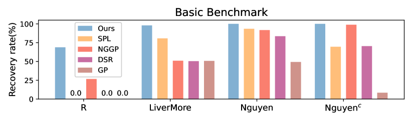
Figure 3: Recover rate (%) of basic benchmarks. Detailed results of each each benchmark can be found in Appendix B.

We performed a comparison of difficult expressions on the four benchmarks listed in Table 1. The results demonstrate that our model performs well on these complex expressions. Our model has the ability to break down complex expressions into stepwise simple expression searches using formal search techniques. For example, the equation $x_{1}^{4}-x_{1}^{3}-0.5x_{2}^{2}+x_{2}$ can be decomposed into the sum of $-0.5x_{2}^{2}$ and $x_{1}^{4}-x_{1}^{3}+x_{2}$. By distilling the equation into the form $x_{1}^{4}-x_{1}^{3}+x_{2}+f(x_{1},x_{2})$ by the results of RL and genetic algorithms, the subsequent search becomes simpler. As a result, our model achieves a 100% recovery rate for these expressions.

Furthermore, we compared the mean recovery rates of all equations on each benchmark (see Figure 3). Our method outperforms other approaches, achieving the highest recovery rates for all expressions.

4.2 Free-falling Balls Dataset

We conducted an experimental evaluation on the free-falling balls dataset to assess the parametric learning capability of our model. The dataset consisted of experimental data of balls dropped from a bridge, as described in a previous study [34]. The dataset comprised 20-30 observations of ball throw heights within the first 2 seconds, aiming to learn the equation governing ball drop and predict the height between 2 and 3 seconds. Since an exact solution for this dataset is not available, we employed the mean squared error (MSE) as our evaluation metric.

Table 2: MSE of free-falling balls dataset. More detailed data on the equations generated by different models can be found in Appendix C.

BenchMark	Ours	Ours∗	SPL	M-A	M-B	M-C
baseball	0.053	0.068	0.300	2.798	94.589	3.507
blue basketball	0.008	0.027	0.457	0.513	69.209	2.227
bowling ball	0.014	0.034	0.003	0.33	87.02	3.167
golf ball	0.006	0.041	0.009	0.214	86.093	1.684
green basketball	0.094	0.045	0.088	0.1	85.435	1.604
tennis ball	0.284	0.068	0.091	0.246	72.278	0.161
volleyball	0.033	0.025	0.111	0.574	80.965	0.76
whiffle ball 1	0.038	0.660	1.58	1.619	65.426	0.21
whiffle ball 2	0.041	0.068	0.099	0.628	58.533	0.966
yellow whiffle ball	1.277	1.080	0.428	17.341	44.984	2.57
orange whiffle ball	0.031	0.368	0.745	0.379	36.765	3.257
Average	0.173	0.242	0.356	2.24	71.02	1.828

We consider two sets of RSRM models, the standard one and the one (named RSRM*) that follows the expression form $c_{4}x^{3}+c_{3}x^{2}+x_{2}x+c_{1}+f(x)$. We compared these models with the baseline method SPL [3], since other models like NGGP [18], GP [24], DGSR [19], and AIFeynman [16] tend to have large generalization errors due to the limited data points (20-30 per training set) in the falling balls benchmark given the fact that the exact solution is unknown.

Three physics models derived from mathematical principles were selected as baseline models for this experiment, and the unknown constant coefficient values were estimated using Powell’s conjugate direction method. The equations of the baseline models are presented as follows. M-A: $h(t)=c_{1}t^{3}+c_{2}t^{2}+c_{3}t+c_{4}$, M-B: $h(t)=c_{1}\exp(c_{2}t)+c_{3}t+c_{4}$, and M-C: $h(t)=c_{1}\log(\cosh(c_{2}t))+c_{3}$.

The results (see Table 2) show that in most cases, the RSRM model performs better than SPL. The RSRM model can successfully find the equation of motion for uniformly accelerated linear motion ($c_{1}x^{2}+c_{2}x+c_{3}+f(x)$) and search for additional terms to minimize the training error. This leads to improved results compared to SPL. However, there are cases where RSRM makes mistakes, such as obtaining expressions in the form of $c_{1}\cos(x)^{2}+c_{2}+f(x)$ when searching for the yellow whiffle ball. This increases the generalization error and reduces the overall effectiveness compared to SPL. Overall, RSRM outperforms SPL in physics equation discovery, demonstrating its effectiveness in solving parametric learning tasks on the free-falling balls dataset.

4.3 Generalization Performance Test

To compare the generalization ability of our model with other methods, we conducted an experiment on generalization performance. The dataset was generated using the cumulative distribution function (CDF) defined in as follows, with varying means ($\mu$) and variances ($\sigma$). The dataset consisted of 201 points spanning the range from $-$100 to 100.

$$F(x,\mu,\sigma)=\int_{-\infty}^{x}\frac{1}{\sqrt{2\pi\sigma}}e^{\frac{-(t-\mu)^{2}}{2}}dt.$$ (3)

Considering the limited capability of the SPL model [3] to learn very complex equations, we selected NGGP [18] as the appropriate baseline for evaluating generalization ability. In addition to our model, we included several baselines for comparison: cubic splines [35], NGGP [18], and Multilayer Perceptron (MLP) implemented with PyTorch [36]. The models were trained based on the datasets sampled in the range of [0, 100]. The rest dataset within the range of [-100, 0) was used to test the generalization ability of each model. We then evaluated and compared the performance of our model and the baselines.

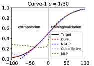
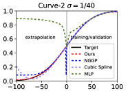
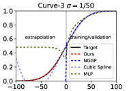
Figure 4: Generalization test experiment. The MSE metrics and the mathematical functions discovered during the generalization experiments are given in Appendix D.

The results of the experiment, shown in Figure 4, demonstrate that our model outperforms the baseline methods in terms of generalization ability. The curves fitted by our model exhibit better accuracy and capture the underlying patterns in the data more effectively. Moreover, the equations generated by our model possess several advantages over the baseline methods (see Appendix Table S8), which are not only easier to calculate, but also more parsimonious in terms of their mathematical expressions.

5 Ablation Study

Table 3: Recovery rate (%) of the ablation study on the LiverMore dataset. The specific recovery rate values are further shown in Appendix E.

Equation	Ours	Model A	Model B	Model C	Model D
$\mathrm{sin}(x_{1}^{2})\mathrm{cos}(x_{1})-2$	100	100	100	6	100
$\mathrm{sin}(x_{1}^{2})\mathrm{cos}(x_{1})-5$	100	89	60	0	100
$\mathrm{sin}(x_{1}^{3})\mathrm{cos}(x_{1}^{2})-1$	55	20	0	0	55
$\mathrm{sinh}(x_{1})$	100	100	100	100	10
$\mathrm{cosh}(x_{1})$	100	100	100	100	3
$\sum_{k=1}^{9}x^{k}$	100	83	100	88	100
$x_{1}^{1/3}$	100	100	100	67	100
$x_{1}^{2/5}$	100	100	100	12	100
Average:	97.95	94.36	93.64	80.45	89.45

We conducted a series of ablation experiments on the LiverMore dataset, testing the ablation of double Q-learning (Model A), the ablation of the MCTS algorithm (Model B), and the ablation of the search form (Model C), and the ablation of the pre-processing step (Model D). We list some of the expressions affected by the performance of the model in Table 3.

When the double Q-learning module is removed, Model A with only MCTS experiences a decrease in knowledge from previous iterations. This results in reduced search efficiency but increased diversity. As a result, we observe a decrease in performance for equations like $\sum_{k=1}^{9}x^{k}$, while equations like $\mathrm{sin}(x_{1}^{3})\mathrm{cos}(x_{1}^{2})-1$ show improved performance. On the other hand, when the MCTS module is removed, Model B with pure double A-learning tends to overfit more quickly. Consequently, it struggles to produce the most challenging equations, such as $\mathrm{sin}(x_{1}^{3})\mathrm{cos}(x_{1}^{2})-1$. Similarly, the absence of the expression form search module in Model C limits its ability to discover complex expressions with simple forms, such as $x_{1}^{1/3}$ and $\mathrm{sin}(x_{1}^{3})\mathrm{cos}(x_{1}^{2})-1$. Lastly, Model D, without the preprocessing module, suffers a significant reduction in its ability to search for odd and even functions like $\mathrm{sinh}(x_{1})$.

These observations highlight the importance and usefulness of all the modules in our approach. Each module contributes to the overall performance and enables the model to tackle different types of equations effectively.

6 Conclusion

We have proposed a novel model that integrates reinforcement learning techniques, GP, and a modulated sub-tree discovery block to improve the search process for mathematical expressions. Our model outperforms state-of-the-art baselines in accurately recovering the exact representation of the baseline tasks and physical equation finding and demonstrates superior generalization capabilities. However, one limitation of our current model is the lack of flexibility in setting the expression form, which restricts its adaptability to different problem domains. We anticipate future advancements in more flexible methods, potentially incorporating neural networks to generate slots for symbolic regression. Furthermore, we believe that our approach has the potential to be extended to other domains, such as reinforcement learning control tasks. By applying our method to diverse areas, we aim to enhance the performance and applicability of symbolic regression techniques.

APPENDIX

Appendix A Model Setting

In this section, we give more details about the settings of our models. The full set of hyperparameters can be seen in Table S1.

Table S1: Hyperparameters of our model

Name	Abbreviation	Value
RL parameters
Minimum expression lengths	$l_{min}$	$4$
Maximum expression lengths	$l_{max}$	$35$
Maximum number of parameters	$c_{max}$	$10$
Length discount rate	$\eta$	$0.99$
Training rounds	$t_{r}$	$50$
UCT constant	$c$	$\sqrt{2}$
Minimum selected times	$n_{0}$	$3$
Learning rate of double Q-learning	$lr$	$10^{-3}$
Genetic Programming parameters
GP rounds	$t_{gp}$	$30$
GP population	$p_{gp}$	$500$
GP number of best expressions	$l_{b}$	$20$
GP Mate rate	$p_{mate}$	$0.5$
GP Mutate rate	$p_{mutate}$	$0.5$
MSDB parameters
Error of Symmetry	$E_{sym}$	$10^{-5}$
Selection ratio	$k_{s}$	$0.1$
Expression percentage ratio	$k_{p}$	$0.1$
Maximum select number	$N$	$5$

Expression constraint: In this study, we incorporate a prior constraint inspired by the DSR method to effectively reduce the search space for expressions. The following constraints are applied:

• Length constraint: The length of expressions is restricted within pre-defined minimum and maximum values. If the current length falls below the minimum threshold, variables ( $x$, $y$, $C$, etc. ) and parameters will not be generated. Conversely, if the current length, combined with the number of nodes to be generated, reaches the maximum length, only these nodes will be considered.

• Unary operator constraint: The direct successor node of a unary operator should not be the inverse of that same operator. This constraint ensures that the generated expressions adhere to the intended structure and prevent redundant combinations.

• Trigonometric function constraint: The successor node of a trigonometric function node should not be another trigonometric function. This constraint prevents the generation of expression structures that lead to unnecessary complexity or redundancy.

• Maximum parameter limit: A specified maximum number of parameters is imposed to control the complexity of the expressions and prevent overfitting.

By applying these expression constraints, we aim to enhance the search efficiency and guide the generation of meaningful expressions that align with the desired properties of the target problem.

Appendix B Basic Benchmark Result

B.1 Baseline Setting

In this section, we give more details about the settings of baselines( SPL, NGGP, DSR, GP ). The full set of hyperparameters can be seen below.

• SPL: In line with the original paper, we maintain the same parameter settings for SPL. The discount rate is set to $\eta=0.9999$, and the candidate operators include addition ($+$), subtraction ($-$), multiplication ($\times$), division ($\div$), cosine ($\cos(\cdot)$), sine ($\sin(\cdot)$), exponential ($\exp(\cdot)$), natural logarithm ($\log(\cdot)$), and square root ($\sqrt{\cdot}$). Other parameter values are as follows: Maximum Module Transplantation: $20$, Episodes Between Module Transplantation: $50000$, Maximum Tree Size: $50$, and Maximum Augmented Grammars: $5$.

• DSR/NGGP: In our study, we adopt the standard parameter configurations as provided in the publicly available implementation of Deep Symbolic Optimization (DSO). This approach entails adjusting two primary hyperparameters. The entropy coefficient is set $\lambda H=0.05$ and the risk factor is set $\epsilon=0.005$. Candidate operators are the same as those employed in the SPL. Additionally, NGGP incorporates other hyperparameters related to hybrid methods based on genetic programming. The specific values are listed in Table S2.

• Genetic Programming (GP): We employ the gplearn library for GP-based methods. The hyperparameters for genetic programming are identical to those presented in Table S2.

Table S2: Genetic Programming Hyperparameters on baselines

Name	Value
Rounds	$20$
Population	$1000$
Mate rate	$0.5$
Mutate rate	$0.5$

B.2 Nyugen Benchmark Result

In this section, we provide additional details about the results obtained from the Nyugen and Nyugen^c Benchmark experiment.

By referring to Table S3, readers can obtain more detailed information about the performance of each model on each expression, their comparative analysis, and any other relevant insights derived from the experiment.

Table S3: Average Recovery Rate (%) of the Nyugen Benchmark over $100$ parallel runs

Name	Equation	Ours	SPL	NGGP	DSR	GP
Nguyen-1	$x_{1}^{3}+x_{1}^{2}+x_{1}$	100	100	100	100	99
Nguyen-2	$x_{1}^{4}+x_{1}^{3}+x_{1}^{2}+x_{1}$	100	100	100	100	90
Nguyen-3	$x_{1}^{5}+x_{1}^{4}+x_{1}^{3}+x_{1}^{2}+x_{1}$	100	100	100	100	34
Nguyen-4	$x_{1}^{6}+x_{1}^{5}+x_{1}^{4}+x_{1}^{3}+x_{1}^{2}+x_{1}$	100	99	100	100	54
Nguyen-5	$\mathrm{sin}(x_{1}^{2})\mathrm{cos}(x_{1})-1$	100	95	80	72	12
Nguyen-6	$\mathrm{sin}(x_{1})+\mathrm{sin}(x_{1}+x_{1}^{2})$	100	100	100	100	11
Nguyen-7	$\mathrm{log}(x_{1}+1)+\mathrm{log}(x_{1}^{2}+1)$	100	100	100	35	17
Nguyen-8	$\sqrt{x_{1}}$	100	100	100	96	76
Nguyen-9	$\mathrm{sin}(x_{1})+\mathrm{sin}(x_{2}^{2})$	100	100	100	100	86
Nguyen-10	$\mathrm{sin}(x_{1})\mathrm{cos}(x_{2})$	100	100	100	100	13
Nguyen-11	$x_{1}^{x_{2}}$	100	100	100	100	100
Nguyen-12	$x_{1}^{4}-x_{1}^{3}-0.5x_{2}^{2}+x_{2}$	100	28	21	0	0
Nguyen-$1^{c}$	$3.39x_{1}^{3}+2.12x_{1}^{2}+1.78x_{1}$	100	100	100	100	0
Nguyen-$2^{c}$	$0.48x_{1}^{4}+3.39x_{1}^{3}+2.12x_{1}^{2}+1.78x_{1}$	100	94	100	100	0
Nguyen-$5^{c}$	$\mathrm{sin}(x_{1}^{2})\mathrm{cos}(x_{1})-0.75$	100	95	98	0	1
Nguyen-$7^{c}$	$\mathrm{log}(x_{1}+1.4)+\mathrm{log}(x_{1}^{2}+1.3)$	100	0	100	93	2
Nguyen-$8^{c}$	$\sqrt{1.23x_{1}}$	100	100	100	100	56
Nguyen-$9^{c}$	$\mathrm{sin}(1.5x_{1})+\mathrm{sin}(0.5x_{2}^{2})$	100	98	96	0	0
Nguyen-$10^{c}$	$\mathrm{sin}(1.5x_{1})\mathrm{cos}(0.5x_{2})$	100	0	100	100	0
	Average:	100.00	84.68	94.47	78.74	29.00

B.3 LiverMore Benchmark Result

In this section, we provide additional details about the results obtained from the LiverMore Benchmark experiment.

By referring to Table S4, readers can obtain more detailed information about the performance of each model on each expression, their comparative analysis, and any other relevant insights derived from the experiment.

Table S4: Average Recovery Rate (%) of the LiverMore Benchmark over $100$ parallel runs

Name	Equation	Ours	SPL	NGGP	DSR	GP
Livermore-1	$1/3+x_{1}+\mathrm{sin}(x_{1})$	100	94	100	67	100
Livermore-2	$\mathrm{sin}(x_{1}^{2})\mathrm{cos}(x_{1})-2$	100	29	61	26	1
Livermore-3	$\mathrm{sin}(x_{1}^{3})\mathrm{cos}(x_{1}^{2})-1$	55	50	2	0	0
Livermore-4	$\mathrm{log}(x_{1}+1)+\mathrm{log}(x_{1}^{2}+x_{1})+\mathrm{log}(x_{1})$	100	61	100	72	100
Livermore-5	$x_{1}^{4}-x_{1}^{3}+x_{1}^{2}-x_{2}$	100	100	100	55	100
Livermore-6	$4x_{1}^{4}+3x_{1}^{3}+2x_{1}^{2}+x_{1}$	100	8	100	100	100
Livermore-7	$\mathrm{sinh}(x_{1})$	100	18	24	0	0
Livermore-8	$\mathrm{cosh}(x_{1})$	100	6	30	0	0
Livermore-9	$\sum_{i=1}^{9}x_{1}^{i}$	100	21	99	18	0
Livermore-10	$6\mathrm{sin}(x_{1})\mathrm{cos}(x_{2})$	100	75	100	70	23
Livermore-11	$(x_{1}^{2}x_{2}^{2})/(x_{1}+x_{2})$	100	0	100	78	95
Livermore-12	$x_{1}^{5}/x_{2}^{3}$	100	100	100	13	100
Livermore-13	$x_{1}^{1/3}$	100	12	100	59	0
Livermore-14	$x_{1}^{3}+x_{1}^{2}+x_{1}+\mathrm{sin}(x_{1})+\mathrm{sin}(x_{1}^{2})$	100	100	100	91	100
Livermore-15	$x_{1}^{1/5}$	100	0	100	28	2
Livermore-16	$x_{1}^{2/5}$	100	0	26	0	0
Livermore-17	$4\mathrm{sin}(x_{1})\mathrm{cos}(x_{2})$	100	89	100	100	84
Livermore-18	$\mathrm{sin}(x_{1}^{2})\mathrm{cos}(x_{1})-5$	100	18	33	37	0
Livermore-19	$x_{1}^{5}+x_{1}^{4}+x_{1}^{2}+x_{1}$	100	89	100	100	100
Livermore-20	$\mathrm{exp}(-x_{1}^{2})$	100	100	100	100	100
Livermore-21	$\sum_{i=1}^{8}x_{1}^{i}$	100	52	100	13	12
Livermore-22	$\mathrm{exp}(-0.5x_{1}^{2})$	100	100	100	82	100
	Average	97.95	51.0	80.68	50.41	50.77

B.4 R Benchmark Result

In this section, we provide additional details about the results obtained from the R Rational Benchmark experiment.

By referring to Table S5, readers can obtain more detailed information about the performance of each model on each expression, their comparative analysis, and any other relevant insights derived from the experiment.

Table S5: Average Recovery Rate (%) of the R Rational Benchmark over $100$ parallel runs

Name	Equation	Ours	SPL	NGGP	DSR	GP
R0-1	$(x_{1}+1)^{3}/(x_{1}^{2}-x_{1}+1)$	5	0	15	0	0
R0-2	$(x_{1}^{5}-3x_{1}^{3}+1)/(x_{1}^{2}+1)$	80	0	40	0	0
R0-3	$(x_{1}^{5}+x_{1}^{6})/(x_{1}^{4}+x_{1}^{3}+x_{1}^{2}+x_{1}+1)$	100	0	100	0	0
R∗-1	$(x_{1}+1)^{3}/(x_{1}^{2}-x_{1}+1)$	48	0	2	0	0
R∗-2	$(x_{1}^{5}-3x_{1}^{3}+1)/(x_{1}^{2}+1)$	89	0	0	0	0
R∗-3	$(x_{1}^{5}+x_{1}^{6})/(x_{1}^{4}+x_{1}^{3}+x_{1}^{2}+x_{1}+1)$	91	0	3	0	0
	Average	68.83	0.0	26.67	0.0	0.0

Appendix C Free-falling Balls Dataset Result

In this section, we provide additional details about the results obtained from the Falling-Balls dataset experiment.To improve the performance of the SPL model, we incorporated the operators $\log(\cosh(\cdot))$. This addition aimed to enhance the model’s ability to capture the underlying patterns in the data.

The complete results of the experiment, including the functions found, can be found in Table S6.

Table S6: Functions generated in Falling-Balls Experiment

Name	Model	Equation
baseball	Ours	$-4.43t^{2}+0.36\sin(t^{2}+1.51)^{2}+47.35$
	Model A	$0.09t^{3}-5.47t^{2}+2.47t+46.52+\cos(t^{2}-2.5t)^{0.5}$
	SPL	$-4.54t^{2}+0.625t+47.8$
blue basket ball	Ours	$-1.66t^{3}-4.95t^{2}\cos(\sqrt{t})+46.46$
	Model A	$-0.1t^{3}-4.49t^{2}+37.54t+46.49-t(\cos(t)+36.77)$
	SPL	$-0.25t^{4}+t^{3}-5.11t^{2}+46.47$
bowling ball	Ours	$-4.63t^{2}+\sin(0.83t)\sin(t)+46.13$
	Model A	$0.18t^{3}-6.0t^{2}+2.15t+45.43+|t-0.62|$
	SPL	$-0.285t^{3}-3.82t^{2}+4.14\times 10^{-5}\exp(20.74t^{2}-12.45t^{3})+46.1$
golf ball	Ours	$-0.09t^{3}-4.44t^{2}+5.26\times 10^{-5}t/\log(t)+49.51$
	Model A	$-2.18t^{3}+11.75t^{2}+1.96t+25.86-2.36\exp(t)+25.98\cos(t)$
	SPL	$-4.9633t^{2}+\log(\cosh(t))+49.5087$
green basket ball	Ours	$46.34-4.15t^{2}$
	Model A	$-0.09t^{3}-4.59t^{2}+1.6t+45.26+(\frac{0.02\sqrt{t}}{t-\exp(\cos(t))}-t+1)\cos(t)$
	SPL	$-4.1465t^{2}+45.9087+\log(\cosh(1))$
tennis ball	Ours	$47.78\cos(0.43t-0.02)$
	Model A	$0.33t^{3}-4.9t^{2}+0.66t+47.74$
	SPL	$-4.0574t^{2}+\log(\cosh(0.121t^{3}))+47.8577$
volleyball	Ours	$48.15-3.67(t+0.03)^{2}$
	Model A	$1.59t^{3}-11.1t^{2}+0.93t+58.53-10.53\cos(t)$
	SPL	$-3.78t^{2}+48.0744$
whiffle ball1	Ours	$-t^{2}(3.83-0.31t)+47.07$
	Model A	$-0.08t^{3}-2.17t^{2}-1.69t+46.29+\sqrt{t+\sin(3t)}$
	SPL	$-t^{3}+4.16t^{2}+47.01\exp(-0.15t^{2})$
whiffle ball2	Ours	$-2.18t^{2}+0.1t\cos(t)+3.35\cos(t)+43.88$
	Model A	$0.46t^{3}-4.39t^{2}+0.19t+47.26-0.05\cos(\exp(t))$
	SPL	$65.86\exp(-0.0577t^{2})-18.61$
yellow whiffle ball	Ours	$(\cos(1.75t)+47.59)\cos(0.36t)$
	Model A	$-0.27t^{3}-2.58t^{2}-2.5t+48.25+(t+0.41)\exp(\sqrt{t+t^{2}-2\sqrt{t^{3}}})$
	SPL	$(148.99-14.58t^{2}+48.96\log(\cosh(x)))/(\log(\cosh(t))+3.065)$
orange whiffle ball	Ours	$-17.82t-33.11/\exp(t)^{0.5}+80.94$
	Model A	$0.42t^{3}-3.81t^{2}-1.4t+47.84$
	SPL	$-1.66t+47.86\exp(-0.0682t^{2})$

Appendix D Generalization Experiment Result

In this section, we provide further details regarding the Generalization Benchmark on Gaussian results.

Each dataset is divided into three subsets: a training set, a test set, and a validation set. The training set comprises points ranging from $30$ to $80$, while the test set consists of points ranging from $10$ to $25$. The validation set covers a broader range, spanning from $0$ to $100$.

To evaluate the performance of our approach and compare it with baselines, we define the following settings for each method:

• Ours: The training set is utilized for generating expressions and calculating the corresponding rewards. The test set is employed to evaluate the quality of the generated expressions. Finally, the validation set is employed to select the most promising expressions from the outputs.

• NGGP: Both the training set and the test set are used for generating expressions and computing rewards. The HallOfFame, which contains the best expressions, is then leveraged to choose expressions using the validation set.

• Linear regression: The training set and the test set are employed for training the linear regression model.

• Cubic spline: The training set and the test set are used to train the cubic spline model.

• Deep learning: In the deep learning approach, we employ a Multilayer Perceptron (MLP) architecture with one input, one output, and a hidden layer ranging in size from 30 to 50. We set learning rate to $10^{-3}$ and train 100 epoches. We experiment with different configurations of the hidden layer and select the model that yields the best performance. The MLP is trained using the training set, and the test set is used to evaluate the performance of each model. By varying the size of the hidden layer, we aim to find the optimal architecture that achieves the highest accuracy or lowest error on the given task.

The full results of the generalization experiment can be found in Table S7. This table presents a detailed overview of the performance of the model and the baselines. Additionally, Table S8 presents the equations discovered by the model and the baselines.

Table S7: Mean Squared Error (MSE) of each method and each part of the curve in the Generalization Experiment

Name	Ours	NGGP	Linear	Cubic Spline	MLP
total error on curve 1	$\mathbf{1.05\times 10^{-5}}$	$0.00215$	$0.0114$	$0.000381$	$0.0142$
total error on curve 2	$\mathbf{9.79\times 10^{-6}}$	$0.00163$	$0.0297$	$0.00162$	$0.261$
total error on curve 3	$\mathbf{2.61\times 10^{-7}}$	$0.327$	$0.0821$	$0.00563$	$0.0762$
extrapolation error on curve 1	$\mathbf{1.65\times 10^{-5}}$	$0.00429$	$0.0215$	$0.000758$	$0.0278$
extrapolation error on curve 2	$\mathbf{1.41\times 10^{-5}}$	$0.00324$	$0.0565$	$0.00323$	$0.518$
extrapolation error on curve 3	$\mathbf{2.67\times 10^{-7}}$	$0.65$	$0.158$	$0.0112$	$0.151$
validation error on curve 1	$4.46\times 10^{-6}$	$\mathbf{2.59\times 10^{-10}}$	$0.00129$	$2.76\times 10^{-10}$	$0.000532$
validation error on curve 2	$5.45\times 10^{-6}$	$\mathbf{1.08\times 10^{-10}}$	$0.00265$	$2.87\times 10^{-9}$	$0.00177$
validation error on curve 3	$2.55\times 10^{-7}$	$2.94\times 10^{-5}$	$0.00518$	$\mathbf{3.75\times 10^{-8}}$	$0.00106$
test error on curve 1	$6.95\times 10^{-6}$	$9.09\times 10^{-12}$	$0.000545$	$\mathbf{<1\times 10^{-12}}$	$0.000253$
test error on curve 2	$2.25\times 10^{-7}$	$\mathbf{<1\times 10^{-12}}$	$0.00127$	$\mathbf{<1\times 10^{-12}}$	$0.00344$
test error on curve 3	$8.8\times 10^{-8}$	$\mathbf{<1\times 10^{-12}}$	$0.00272$	$\mathbf{<1\times 10^{-12}}$	$0.00358$
training error on curve 1	$3.88\times 10^{-6}$	$3.57\times 10^{-12}$	$0.000254$	$\mathbf{<1\times 10^{-12}}$	$6.93\times 10^{-5}$
training error on curve 2	$1.26\times 10^{-6}$	$\mathbf{<1\times 10^{-12}}$	$0.000524$	$\mathbf{<1\times 10^{-12}}$	$8.6\times 10^{-5}$
training error on curve 3	$3.34\times 10^{-7}$	$7.14\times 10^{-12}$	$0.000905$	$\mathbf{<1\times 10^{-12}}$	$7.9\times 10^{-5}$

Table S8: Functions generated in Generalization Experiment. Our functions are easier to calculate and shorter than NGGP’s.

Name	Model	Equation
curve-1	Ours	$0.503+(117.088x)/(x^{2}+14702)$
	NGGP	$\cos(\exp((0.49x\log(0.028x+29.5/(0.039x+9.82))-2.78)/(0.115x-60.5)))$
curve-2	Ours	$(6.08x+0.785)/(0.0639x^{2}+615.179)+0.50003$
	NGGP	$\cos(2.95\exp(-0.68\exp(0.41\exp(5.5x\exp(24.67/(115.6\exp((4.75x+13.3)/x)+3.2))/(2x+214.3)))))$
curve-3	Ours	$(x\sin(371.57/(13928/x+x))+x)/(0.0024+2x)$
	NGGP	$\cos(\log(1+1.67\exp(-1.56/(\exp(17.7\exp(\exp((-12.9+4.95\log(x)/x)/x))/x)-1.16+0.656/x))))$

Appendix E Ablation Experiment Result

In this section, we provide more detailed information about the results obtained from the ablation experiment on LiverMore benchmark. The full results of the ablation experiment can be found in Table S9. This table presents a comprehensive overview of the performance of the model under different ablation settings.

Table S9: Average Recovery Rate (%) of the Ablation Experiment over $100$ parallel runs

Name	Equation	Ours	ModelA	ModelB	ModelC	ModelD
Livermore-1	$1/3+x_{1}+\mathrm{\sin}(x_{1})$	100	100	100	100	100
Livermore-2	$\mathrm{sin}(x_{1}^{2})\mathrm{cos}(x_{1})-2$	100	100	100	6	100
Livermore-3	$\mathrm{sin}(x_{1}^{3})\mathrm{cos}(x_{1}^{2})-1$	55	20	0	0	55
Livermore-4	$\mathrm{log}(x_{1}+1)+\mathrm{log}(x_{1}^{2}+x_{1})+\mathrm{log}(x_{1})$	100	100	100	100	100
Livermore-5	$x_{1}^{4}-x_{1}^{3}+x_{1}^{2}-x_{2}$	100	100	100	100	100
Livermore-6	$4x_{1}^{4}+3x_{1}^{3}+2x_{1}^{2}+x_{1}$	100	100	100	100	100
Livermore-7	$\mathrm{sinh}(x_{1})$	100	100	100	100	10
Livermore-8	$\mathrm{cosh}(x_{1})$	100	100	100	100	3
Livermore-9	$\sum_{i=1}^{9}x_{1}^{i}$	100	83	100	88	100
Livermore-10	$6\mathrm{sin}(x_{1})\mathrm{cos}(x_{2})$	100	100	100	100	100
Livermore-11	$(x_{1}^{2}x_{2}^{2})/(x_{1}+x_{2})$	100	91	100	100	100
Livermore-12	$x_{1}^{5}/x_{2}^{3}$	100	100	100	100	100
Livermore-13	$x_{1}^{1/3}$	100	100	100	67	100
Livermore-14	$x_{1}^{3}+x_{1}^{2}+x_{1}+\mathrm{sin}(x_{1})+\mathrm{sin}(x_{1}^{2})$	100	100	100	100	100
Livermore-15	$x_{1}^{1/5}$	100	100	100	97	100
Livermore-16	$x_{1}^{2/5}$	100	100	100	12	100
Livermore-17	$4\mathrm{sin}(x_{1})\mathrm{cos}(x_{2})$	100	100	100	100	100
Livermore-18	$\mathrm{sin}(x_{1}^{2})\mathrm{cos}(x_{1})-5$	100	89	90	0	100
Livermore-19	$x_{1}^{5}+x_{1}^{4}+x_{1}^{2}+x_{1}$	100	100	100	100	100
Livermore-20	$\mathrm{exp}(-x_{1}^{2})$	100	100	100	100	100
Livermore-21	$\sum_{i=1}^{8}x_{1}^{i}$	100	100	100	100	100
Livermore-22	$\mathrm{exp}(-0.5x_{1}^{2})$	100	100	100	100	100
	Average	97.95	94.68	95.0	80.45	89.45

References

- [1] Silviu-Marian Udrescu and Max Tegmark. Ai feynman: A physics-inspired method for symbolic regression. Science Advances, 6(16):eaay2631, 2020.
- [2] Ziming Liu and Max Tegmark. Machine learning conservation laws from trajectories. Physical Review Letters, 126(18):180604, 2021.
- [3] Fangzheng Sun, Yang Liu, Jian-Xun Wang, and Hao Sun. Symbolic physics learner: Discovering governing equations via monte carlo tree search. arXiv preprint arXiv:2205.13134, 2022.
- [4] Yiqun Wang, Nicholas Wagner, and James M Rondinelli. Symbolic regression in materials science. MRS Communications, 9(3):793–805, 2019.
- [5] Eurika Kaiser, J Nathan Kutz, and Steven L Brunton. Sparse identification of nonlinear dynamics for model predictive control in the low-data limit. Proceedings of the Royal Society A, 474(2219):20180335, 2018.
- [6] Fangzheng Sun, Yang Liu, and Hao Sun. Physics-informed spline learning for nonlinear dynamics discovery. arXiv preprint arXiv:2105.02368, 2021.
- [7] Zhao Chen, Yang Liu, and Hao Sun. Physics-informed learning of governing equations from scarce data. Nature communications, 12(1):6136, 2021.
- [8] Kathleen Champion. From data to dynamics: discovering governing equations from data. PhD thesis, 2019.
- [9] Georg Martius and Christoph H Lampert. Extrapolation and learning equations. arXiv preprint arXiv:1610.02995, 2016.
- [10] Subham Sahoo, Christoph Lampert, and Georg Martius. Learning equations for extrapolation and control. In International Conference on Machine Learning, pages 4442–4450. PMLR, 2018.
- [11] J. E. Hopcroft, R. Motwani, and J. D. Ullman. Automata theory, languages, and computation. Pearson Education, 2006.
- [12] Michael Schmidt and Hod Lipson. Distilling free-form natural laws from experimental data. Science, 324(5923):81–85, 2009.
- [13] Douglas Adriano Augusto and Helio JC Barbosa. Symbolic regression via genetic programming. In Proceedings. Vol. 1. Sixth Brazilian Symposium on Neural Networks, pages 173–178. IEEE, 2000.
- [14] Steven Gustafson, Edmund K Burke, and Natalio Krasnogor. On improving genetic programming for symbolic regression. In 2005 IEEE Congress on Evolutionary Computation, volume 1, pages 912–919. IEEE, 2005.
- [15] Mojtaba Valipour, Bowen You, Maysum Panju, and Ali Ghodsi. Symbolicgpt: A generative transformer model for symbolic regression. arXiv preprint arXiv:2106.14131, 2021.
- [16] Silviu-Marian Udrescu, Andrew Tan, Jiahai Feng, Orisvaldo Neto, Tailin Wu, and Max Tegmark. Ai feynman 2.0: Pareto-optimal symbolic regression exploiting graph modularity. Advances in Neural Information Processing Systems, 33:4860–4871, 2020.
- [17] Brenden K Petersen, Mikel Landajuela, T Nathan Mundhenk, Claudio P Santiago, Soo K Kim, and Joanne T Kim. Deep symbolic regression: Recovering mathematical expressions from data via risk-seeking policy gradients. arXiv preprint arXiv:1912.04871, 2019.
- [18] T Nathan Mundhenk, Mikel Landajuela, Ruben Glatt, Claudio P Santiago, Daniel M Faissol, and Brenden K Petersen. Symbolic regression via neural-guided genetic programming population seeding. arXiv preprint arXiv:2111.00053, 2021.
- [19] Samuel Holt, Zhaozhi Qian, and Mihaela van der Schaar. Deep generative symbolic regression. In International Conference on Learning Representations, 2022.
- [20] Pierre-Alexandre Kamienny, Stéphane d’Ascoli, Guillaume Lample, and François Charton. End-to-end symbolic regression with transformers. arXiv preprint arXiv:2204.10532, 2022.
- [21] Wenqiang Li, Weijun Li, Linjun Sun, Min Wu, Lina Yu, Jingyi Liu, Yanjie Li, and Songsong Tian. Transformer-based model for symbolic regression via joint supervised learning. In The Eleventh International Conference on Learning Representations, 2022.
- [22] Hado Hasselt. Double q-learning. Advances in neural information processing systems, 23, 2010.
- [23] Rémi Coulom. Efficient selectivity and backup operators in monte-carlo tree search. In International Conference on Computers and Games, 2006.
- [24] Trevor Stephens. Genetic programming in python, with a scikit-learn inspired api: gplearn. 2016.
- [25] John R Koza. Genetic programming as a means for programming computers by natural selection. Statistics and computing, 4:87–112, 1994.
- [26] David Silver, Julian Schrittwieser, Karen Simonyan, Ioannis Antonoglou, Aja Huang, Arthur Guez, Thomas Hubert, Lucas Baker, Matthew Lai, Adrian Bolton, et al. Mastering the game of go without human knowledge. nature, 550(7676):354–359, 2017.
- [27] John Wiley Roger Fletcher and Sons. Practical methods of optimization. 2013.
- [28] Pauli Virtanen, Ralf Gommers, Travis E Oliphant, Matt Haberland, Tyler Reddy, David Cournapeau, Evgeni Burovski, Pearu Peterson, Warren Weckesser, Jonathan Bright, et al. Scipy 1.0: fundamental algorithms for scientific computing in python. Nature methods, 17(3):261–272, 2020.
- [29] Aaron Meurer, Christopher P Smith, Mateusz Paprocki, Ondřej Čertík, Sergey B Kirpichev, Matthew Rocklin, AMiT Kumar, Sergiu Ivanov, Jason K Moore, Sartaj Singh, et al. Sympy: symbolic computing in python. PeerJ Computer Science, 3:e103, 2017.
- [30] Edwin Catmull and Raphael Rom. A class of local interpolating splines. In Computer aided geometric design, pages 317–326. Elsevier, 1974.
- [31] Nguyen Quang Uy, Nguyen Xuan Hoai, Michael O’Neill, Robert I McKay, and Edgar Galván-López. Semantically-based crossover in genetic programming: application to real-valued symbolic regression. Genetic Programming and Evolvable Machines, 12:91–119, 2011.
- [32] James McDermott, David R White, Sean Luke, Luca Manzoni, Mauro Castelli, Leonardo Vanneschi, Wojciech Jaskowski, Krzysztof Krawiec, Robin Harper, Kenneth De Jong, et al. Genetic programming needs better benchmarks. In Proceedings of the 14th annual conference on Genetic and evolutionary computation, pages 791–798, 2012.
- [33] Terrell Mundhenk, Mikel Landajuela, Ruben Glatt, Claudio P Santiago, Brenden K Petersen, et al. Symbolic regression via deep reinforcement learning enhanced genetic programming seeding. Advances in Neural Information Processing Systems, 34:24912–24923, 2021.
- [34] Brian M de Silva, David M Higdon, Steven L Brunton, and J Nathan Kutz. Discovery of physics from data: Universal laws and discrepancies. Frontiers in artificial intelligence, 3:25, 2020.
- [35] Nira Dyn, Michael S Floater, and Kai Hormann. Four-point curve subdivision based on iterated chordal and centripetal parameterizations. Computer Aided Geometric Design, 26(3):279–286, 2009.
- [36] Adam Paszke, Sam Gross, Francisco Massa, Adam Lerer, James Bradbury, Gregory Chanan, Trevor Killeen, Zeming Lin, Natalia Gimelshein, Luca Antiga, et al. Pytorch: An imperative style, high-performance deep learning library. Advances in neural information processing systems, 32, 2019.