Graph Analysis Using a GPU-based Parallel Algorithm: Quantum Clustering

Abstract

The article introduces a new method for applying Quantum Clustering to graph structures. Quantum Clustering (QC) is a novel density-based unsupervised learning method that determines cluster centers by constructing a potential function. In this method, we use the Graph Gradient Descent algorithm to find the centers of clusters. GPU parallelization is utilized for computing potential values. We also conducted experiments on five widely used datasets and evaluated using four indicators. The results show superior performance of the method. Finally, we discuss the influence of $\sigma$ on the experimental results.

1 Introduction

Graph Clustering, also known as network clustering, is a technique for partitioning a graph into clusters or communities of nodes based on their structural properties(schaeffer2007graph, ). Graph clustering is used in various applications such as social network analysis, image segmentation, bioinformatics, and more. The goal of graph clustering is to group the nodes in a way to maximizes the similarity within the group and minimizes the similarity between them(zhou2009graph, ). These two similarities are usually measured using various metrics such as modularity, Normalized Mutual Information(NMI), Adjusted Rand Index(ARI) and FowlkesMallows Index(FMI). There are various algorithms for graph clustering, including K-Means(arthur2007k, ), Spectral Clustering(shi2000normalized, ; von2007tutorial, ; stella2003multiclass, ; knyazev2001toward, ), DBSCAN(ester1996density, ; ester1996proceedings, ; schubert2017dbscan, ), Louvain(blondel2008fast, ; dugue2015directed, ), localized community detection algorithm based on label propagation(LPA)(raghavan2007near, ), BIRCH(zhang1996birch, ; zhang1997birch, ), AGENS(zhang2012graph, ; zhang2013agglomerative, ; fernandez2008solving, ), etc. The challenging problem in graph clustering is that we need to cluster its basic structures and use these structures for clustering purposes, which need more efficient clustering algorithms(aggarwal2010survey, ). However, QC is a very effective clustering algorithm to uncover subtle changes in the underlying data.

The Quantum clusteringhorn2001algorithm is a novel clustering method based on the Schrödinger equation. QC calculates the so-called potential function to reveal the structure of the data. While the potential function depends entirely on the parameter $\sigma$ and we discuss the $\sigma$ in section 5. QC has been extensively demonstrated and experimented in our previous work(liu2016analyzing, ), and show its superior performance. In order to find the minimum node in the graph structure, we design a so-called Graph gradient descent(GGD) algorithm and we will describe the algorithm in detail in the section 3.1. in section 4, We demonstrate the performance of QC on five datasets and compare it with six other algorithms.

2 Related works

The graph clustering algorithm can be mainly divided into four categories. i.e, Partition Clustering, Hierarchical Clustering, Density-based Clustering, Model-based Clustering(van2000graph, ). These methods all has its unique advantages and application scenarios. Representative algorithms for each clustering method are shown in Fig. 1. And QC can be regarded as a density-based clustering method.

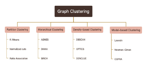
Figure 1: A classification of Graph Clustering;

.

2.1 Partition Clustering

Partition Clustering divides the graph into multiple subgraphs, and each subgraph contains nodes belonging to the same class. This method is usually implemented using spectral clustering methods, such as spectral clustering based on the Laplacian matrix. Spectral clustering can handle clusters with non-convex and irregular shapes, and is robust to noisy data, so it has high application value in practice. In lately work use a new version of the spectral cluster, named Attributed Spectral Clustering (ASC), ASC use the Topological and Attribute Random Walk Affinity Matrix (TARWAM) as a new affinity matrix to calculate the similarity between nodes(berahmand2022novel, )

2.2 Hierarchical Clustering

Hierarchical Clustering is a strategy of cluster analysis to create a hierarchical of clusters. HC first builds a binary tree and node information is stored in each node. The algorithm starts from such a leaf node, gradually traverses towards the root node, and classifies similar nodes into one category(Nielsen2016, ; johnson1967hierarchical, ). Also the algorithm can traverse from the root node to the leaf nodes. This divides HC into two categories, agglomerative (bottom-up) and divisive (top-down)(li2022ensemble, ). (dogan2022k, ) Propose a novel linkage method, named k-centroid link.

2.3 Density-based Clustering

Density-based Clustering is a nonparametric approach where clusters are considered as high density regions of $P(x)$. The steps of density-based clustering is to find the core point(braune2015density, ), and then divide the nodes in the adjacent area into a cluster and assign the border point to the cluster where its adjacent core point is located. Finally, remove noise points. (kriegel2011density, ) Imagine the density-based clusters as the set of points resulting from ”cutting” the probability density function of the data at some density level.

2.4 Model-based Clustering

This method models the graph clustering problem as a probabilistic model and use methods such as EM algorithm and Bayesian inference to learn the model parameters and obtain the clustering results. This method is usually implemented using models such as Gaussian mixture models and latent Dirichlet allocation(mcnicholas2016model, ).

3 Method

In this section, we begin with a description of the fundamentals of Quantum Clustering(liu2016analyzing, ; nasios2007kernel, ; horn2001algorithm, ; horn2001method, ). And then we list the pseudocode of the key steps of the algorithm.

3.1 Algorithm

Quantum Clustering is a new machine learning algorithm based on the Schrödinger equation. In our work, we choose the time-independent Schrödinger equation Eq(1) (feynman1965feynman, ). We use this equation to explore graph structures at a deeper level. The algorithm process can be decomposed into the following steps.

$$H\psi\left(x\right)=\left(-\frac{\hbar^{2}}{2m}\nabla^{2}+v(x)\right)\psi\left(x\right)=E\psi\left(x\right)$$ (1)

Here H denotes Hamiltonian operator, which is an operator that describes the energy of a quantum system. $\psi(x)$ denotes Wave function, which is the fundamental physical quantity that describes a quantum system. and v(x) denotes potential function, which is describing the probability density function of the input data(nasios2007kernel, ). Given a Gaussian wave function Eq(2), use the Schrödinger equation to calculate the potential function. Here $\sigma$ denotes the width parameter.

$$\psi\left(x\right)=\sum_{i}e^{-\left(x-{x}_{i}\right)^{2}/2\sigma^{2}}$$ (2)

Thus, the potential function v(x) could be solved as:

$$v(x) =E+\frac{\sum_{i}(e^{\frac{-(x-x_{i})^{2}}{2\sigma^{2}}}\cdot\frac{(x-x_{i})^{2}}{2\sigma^{2}}-e^{\frac{-(x-x_{i})^{2}}{2\sigma^{2}}}\cdot\frac{1}{2})}{\sum_{i}e^{\frac{-(x-x_{i})^{2}}{2\sigma^{2}}}}$$ (3)

$$=E-\frac{1}{2}+\frac{1}{2\sigma^{2}\psi(x)}\sum_{i}(x-{x}_{i})^{2}e^{\frac{-(x-x_{i})^{2}}{2\sigma^{2}}}$$

$$\approx\frac{1}{2\sigma^{2}\psi(x)}\sum_{i}(x-{x}_{i})^{2}e^{\frac{-(x-x_{i})^{2}}{2\sigma^{2}}}$$

Algorithm 1 Calculating the Potential function for each data point

1:$graph:$ graph structure data set,

2:$data:$ data points, $\sigma:$ width parameter, $n:$ the number of data points

3:$weight\leftarrow$ initial value

4:function POTENTIAL($data(i)$)

5:     $sum1\leftarrow 0$

6:     $sum2\leftarrow 0$

7:     for $j=1\to n$ do

8:         if $data(i,0)=graph(j,0)\And data(i,1)=graph(j,1)\mid data(i,0)=graph(j,1)\And data(i,1)=graph(j,0)$ then

9:              $dist$ = graph(j,2)

10:         end if

11:         $dist$ = weight

12:         $sum1\leftarrow sum1+dist(j)^{2}\cdot e^{-dist(j)^{2}/2\sigma^{2}}$

13:         $sum2\leftarrow sum2+e^{-dist(j)^{2}/2\sigma^{2}}$

14:     end for

15:     $v(data(i))\leftarrow\frac{1}{2\sigma^{2}}\cdot\frac{sum1}{sum2}$

16:     return $v(data(i))$

17:end function

Algorithm 2 Graph gradient decent algorithm

$n$ the number of data points

$POTENTIAL(n)$ potential value of each data points

function GRAPH_GRADIENT_DECENT(node)

     for $i=1\to n$ do

         neighbor $\leftarrow$ adjacent nodes id connected with the node i

         $Min\_Potentials(i)\leftarrow$ Node ID of minimum potential value in neighbor

     end for

     $Min\_Potentials\_Unique\leftarrow$ Remove duplicate elements from $Min\_Potentials$

     for $item\in Min\_Potentials\_Unique$ do

         while $Min\_Potentials(item)\neq item$ do

              for $j=1\to n$ do

                  if $Min\_Potentials(j)=item$ then

                       $Min\_Potentials(j)\leftarrow Min\_Potentials(item)$

                  end if

              end for

              $item\leftarrow Min\_Potentials(item)$

         end while

     end for

     return $Min\_Potentials(n)$

end function

In our study, we use a new optimization algorithm. In this algorithm, we design a gradient descent path for each node in the graph structure to descend to the node with the lowest potential energy. First, each node is a separate cluster Fig. 2 The number on a node represents the potential value of that node. We can find that the potential value of the central node is lower than that of the surrounding nodes. This is also the basic principle that quantum clustering can effectively analyze the graph structure. Second, each node traverses its neighboring nodes looking for the node with the lowest potential value. If the potential value of the node is lower than that of the initial node, the initial node is added to the cluster where the node exists Fig. 2. The pseudocode of this part is embodied in algorithm 2 the time complexity of algorithm 2 depends on the density of the graph structure.

Algorithm 1 and 3 shows the pseudocode of computing the potential function and the basic framework of the whole algorithm. The time complexity of algorithm 1 is $O(n)$, n denoted the size of dataset.

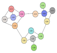
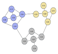
Figure 2: The specific steps of GGD algorithm. (a) First step of the algorithm; (b) Second step of the algorithm;

.

Algorithm 3 Quantum clustering for graph analysis

1:$graph$ graph structure data set,

2:$node:$ node data, $n:$ the number of data points

3:$\sigma\leftarrow$ initial value

4:for $i=1\to n$ do

5:     input each node(i);

6:     calculate the potential of data points by POTENTIAL$(node)$

7:end for

8:assign labels and move each node to its minimum potential energy by $GRAPH\_GRADIENT\_DECENT(node(i))$

3.2 Parallelized by GPU

The most important part of QC algorithm is to calculate the potential value of each data point. So it is very suitable to use GPU for parallelization. In this part, we design experiments to prove its acceleration effect. the GPU version we used for this experiment is A100-SXM4, And the counterpart of CPU version is AMD EPYC 7742 64-Core Processor. We use a series of artificial dataset with different data volumes to complete the experiment. Comparison of GPU and CPU acceleration on a fixed fully-connected graph structure dataset by increasing the number of nodes Fig. 3. All implementation code is visible in the (Wangzhe, ).

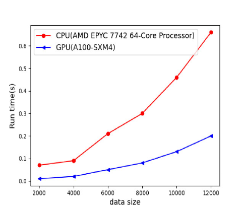
Figure 3: Comparison of GPU and CPU Acceleration;

.

4 Application

4.1 Dataset

To evaluate the effectiveness of the proposed method, we choose five widely-used datasets for this experiment, i.e., Cora(sen2008collective, ), Citeseer(sen2008collective, ), Karate-club(zachary1977information, ), Cora-ML(bojchevski2017deep, ), Wiki(singh2008relational, ). We use the Gephi (bastian2009gephi, ) tool for visualization and result are shown in Fig. 4

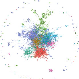
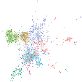
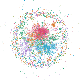
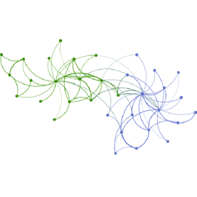
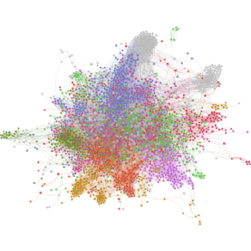
Figure 4: The visualization of datasets for our experiment. ForceAtlas 2 is used as layout demonstration algorithm. (a) Cora dataset; (b) Cora-ML dataset; (c) Citeseer dataset; (d) Karate-club datset; (e) Wiki dataset;

.

4.1.1 Cora&Cora-ML&Citeseer datasets

The Cora dataset is citation network of 2708 scientific publications and 5278 citation relationships covering important topics in the field of computer science, including 7 classes, i.e., machine learning, artificial intelligence, databases, networks, information retrieval, linguistics, and interdisciplinary fields. Each node represents a paper, and the edges between nodes represent citation relationships. The dataset also includes feature vectors for each paper, representing the word frequency of each paper.

The Cora-ML dataset is a variant of the Cora dataset, which is a citation network containing 2995 scientific publications and 8158 citation relationships where each node represents a paper and edges represent citation relationships. The difference between Cora-ML and Cora is that Cora-ML also includes category labels for papers in the machine learning field.

Similar to the Cora dataset, Citeseer dataset consisting of 3327 papers and 4676 citation relationships downloaded from the Citeseer digital library classified into 6 classes. These papers cover important topics in computer science, information science, and communication science, such as machine learning, data mining, information retrieval, and computer vision. Each node represents a paper, and the edges between nodes represent citation relationships. The dataset also includes feature vectors for each paper, representing the word frequency of each paper.

4.1.2 Karate-club dataset

Karate-club dataset represent a social network consisting of 34 nodes and 78 edges. The social network was observed and recorded by Zachary in 1977, and represents the relationships between members of a karate club. This social network is commonly used as a benchmark dataset. In this social network, each node represents a member of the karate club, and the edges represent social connections between members. According to Zachary’s records, the social network eventually split into two communities.

4.1.3 Wiki dataset

The Wiki dataset containing 2405 Wikipedia pages and 12761 link relationships these pages can divided into 17 classes. Each page is represented as a node, and the link relationships between nodes form the graph structure.

4.2 Evaluation method

We use 4 metrics to indices the performance of QC. These 4 metrics can be divided into 2 classes, called internal and external measures. While the former measures is often used when there is no true label, and external measures is often used when there is true label. Next, we introduce these indicators in detail.

4.2.1 Modularity

Modularity(newman2004finding, ) reflects the degree of connection between nodes. A perfect cluster partition result should make the connections within clusters close and the connections between clusters sparse. If the intra-cluster connection is strong and inter-cluster connection is weak. Then the Modularity indicator will be higher, indicating that the quality of community division is better.

The formula for Modularity is as follows:

$$Q=\dfrac{1}{w}\sum_{i,j}\left(A_{ij}-\gamma\dfrac{w_{i}w_{j}}{w}\right)\delta_{c_{i},c_{j}}$$ (4)

Where A is the adjacency of network. $w_{i}$ represents the degree of a node, $w$ is the total weight. $\delta$ is the Kronecker symbol. $\gamma$ is the resolution parameter.

4.2.2 ARI

ARI(hubert1985comparing, ) is a commonly used external evaluation metric in cluster analysis. The interval of ARI value is -1 to 1. Where -1 indicates complete disagreement between the clustering results, 0 indicates the clustering result is the same as random classification, and 1 indicates complete agreement between the clustering results and the true classification.

The formula for ARI is as follows:

$$ARI=\frac{RI-Expected\_RI}{max(RI)-Expected\_RI}$$ (5)

RI is the Rand Index, $Expected_{R}I$ is the expected value of the Rand Index under the null hypothesis of random clustering. The term $(max(RI)-Expected_{R}I)$ is a normalization factor.

4.2.3 FMI

FMI(schutze2008introduction, ) is a measure of the similarity between a clustering result and the true class labels. It is defined as the geometric mean of the precision and recall between the clustering result and the true class labels.

The FMI is calculated as:

$$FMI=\frac{TP}{\sqrt{(TP+FP)*(TP+FN)}}$$ (6)

Where TP is the number of true positive, FP is the number of false positive, FN is the number of false negative.

4.2.4 NMI

NMI(strehl2002cluster, ) is a normalization of the Mutual Information (MI) score to scale the results between 0 (no mutual information) and 1 (perfect correlation) The NMI is calculated as follow:

$$NMI(labels\_true,labels\_pred)=\frac{MI(labels\_true,labels\_pred)}{\sqrt{H(labels\_true)\cdot H(labels\_pred)}}$$ (7)

Where $H$ represents Entropy, MI represents Mutual Information. And $MI(labels\_true,labels\_pred)$ denoted Mutual Information between two sets of labels and can be calculated with following formula:

$$MI(labels\_true,labels\_pred)=\sum_{i=1}^{n}\sum_{j=1}^{m}P(i,j)\log{\frac{P(i,j)}{P(i)P(j)}}$$ (8)

Where $P(i,j)$ denoted the proportion of samples that have a true label of $i$ and a predicted label of $j$ out of the total number of samples. $H(labels_{t}rue)$ and $H(labels_{p}red)$ represent the entropies of the true labels and predicted labels, respectively, and can be calculated as follows:

$$H(labels)=-\sum_{i=1}^{n}P(i)\log{P(i)}$$ (9)

Where $P(i)$ represents the proportion of samples that have a label of $i$ out of the total number of samples.

4.3 Performance comparison

In this part, the CPU version for this experiment is Intel(R) Core(TM) i5-7300HQ. In order to prove the practical value of QC algorithm. We selected six graph clustering algorithms for comparison. The experimental results are shown in Table. 1. We can see that the performance of algorithm Louvain in Cora, Citeseer, Wiki, and Cora_ML dataset is slightly better than that of QC in the table. Louvain algorithm was proposed by Belgian astrophysicist Vincent Blondel and his colleagues in 2008. But in Karate_club dataset, three of the four indicators show that QC is better than the other three algorithms. The Louvain algorithm is slightly better than QC only when the Modularity is used, And the number of clusters due to QC clustering results in the Karate_club dataset is consistent with that in the real label. So we can calculate the F1 value, accuracy rate and Recall rate. The F1 value is 0.91, Recall rate is 1 and Accuracy rate is 0.91. Shows a great advantage. Louvain frist introduced in (blondel2008fast, ), The algorithm uses a greedy algorithm based on modularity optimization, which can quickly detect community structure in large networks. And improved in the paper(dugue2015directed, ). In (raghavan2007near, ) LPA is proposed. Its performance is similar to that of QC.

Table 1: Comparison between QC and the other six algorithms under four performance metrics

		Modularity	NMI	ARI	FMI	Time(s)
Cora	QC	0.634	0.401	0.166	0.285	0.34652
	kmeans	0.017	0.023	0.004	0.422	0.49572
	Louvain	0.812	0.443	0.236	0.358	0.00028
	LPA	0.747	0.389	0.155	0.267	0.00002
	Spectral Clustering	0.009	0.010	-0.006	0.412	1.64937
	AGNES	-0.001	0.001	0.000	0.423	7.32858
	BIRCH	-0.001	0.377	0.001	0.021	0.37595
Citeseer	QC	0.704	0.343	0.073	0.179	0.51841
	kmeans	0.008	0.006	0.000	0.421	0.58689
	Louvain	0.891	0.332	0.101	0.216	0.00025
	LPA	0.834	0.333	0.075	0.180	0.00002
	Spectral Clustering	0.145	0.019	0.006	0.359	3.12891
	AGNES	0.163	0.061	0.002	0.406	13.1427
	BIRCH	0.015	0.352	0.001	0.022	27.4522
Wiki	QC	0.361	0.133	0.029	0.205	0.30821
	kmeans	0.049	0.029	0.003	0.314	0.43979
	Louvain	0.701	0.362	0.165	0.240	0.00026
	LPA	0.308	0.193	0.026	0.301	0.00002
	Spectral Clustering	0.114	0.141	0.021	0.320	0.71140
	AGNES	0.049	0.048	0.006	0.316	4.86280
	BIRCH	0.049	0.483	0.000	0.009	2.88658
Cora_ML	QC	0.620	0.405	0.219	0.327	0.30371
	kmeans	0.008	0.005	-0.002	0.411	0.52607
	Louvain	0.770	0.479	0.312	0.419	0.00025
	LPA	0.718	0.421	0.206	0.322	0.00002
	Spectral Clustering	0.014	0.017	-0.002	0.404	1.89664
	AGNES	0.001	0.001	0.000	0.415	0.89033
	BIRCH	-0.001	0.379	0.002	0.035	4.67560
Karate_club	QC	0.334	0.649	0.668	0.832	0.00223
	kmeans	-0.013	0.093	0.007	0.658	0.01289
	Louvain	0.445	0.588	0.465	0.677	0.00020
	LPA	0.305	0.544	0.504	0.717	0.00002
	Spectral Clustering	0.357	0.469	0.283	0.528	0.03138
	AGNES	0.225	0.244	0.109	0.630	0.00166
	BIRCH	-0.051	0.335	0.008	0.086	0.00130

5 Discussion

In this paper, we extend QC to graph structures. We use a so-called GGD to find the minimum node of the potential function. Based on the above experimental process, this method is simple and effective. We conduct experiments on five datasets and compare them with six other graph clustering algorithms. we can make some conclusions, as a new clustering algorithm, QC has a good performance in graph topology. The implementation of graph clustering in QC relies entirely on $\sigma$. Below, we will provide a detailed explanation of how $\sigma$ affect the results of the algorithm.

We observe the influence on the experimental results by changing the values of the parameters. According to the Fig.5, we find that the growth of $\sigma$ is always accompanied by a ”mutation”. In Cora, Citeseer, Wiki and Cora_ML datasets, This ”mutation” always occurs in the interval between 150 and 160 of the parameter $\sigma$. But in Karate_club dataset ”mutation” occurs in the interval between 190 to 200. This happens because the number of clusters decreases dramatically over a period of time as the delta increases. Generally speaking, the influence of the parameters before and after the mutation on the clustering results is not significant.

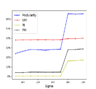
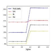
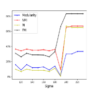
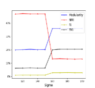
Figure 5: Effect of parameter $\sigma$ on experimental results (a) Cora dataset; (b) Cora-ML dataset; (c) Citeseer dataset; (d) Karate-club datset; (e) Wiki dataset;

.

References

- \bibcommenthead
- (1) Schaeffer, S.E.: Graph clustering. Computer science review 1(1), 27–64 (2007)
- (2) Zhou, Y., Cheng, H., Yu, J.X.: Graph clustering based on structural/attribute similarities. Proceedings of the VLDB Endowment 2(1), 718–729 (2009)
- (3) Arthur, D., Vassilvitskii, S.: K-means++ the advantages of careful seeding. In: Proceedings of the Eighteenth Annual ACM-SIAM Symposium on Discrete Algorithms, pp. 1027–1035 (2007)
- (4) Shi, J., Malik, J.: Normalized cuts and image segmentation. IEEE Transactions on pattern analysis and machine intelligence 22(8), 888–905 (2000)
- (5) Von Luxburg, U.: A tutorial on spectral clustering. Statistics and computing 17, 395–416 (2007)
- (6) Stella, X.Y., Shi, J.: Multiclass spectral clustering. In: Computer Vision, IEEE International Conference On, vol. 2, pp. 313–313 (2003). IEEE Computer Society
- (7) Knyazev, A.V.: Toward the optimal preconditioned eigensolver: Locally optimal block preconditioned conjugate gradient method. SIAM journal on scientific computing 23(2), 517–541 (2001)
- (8) Ester, M., Kriegel, H.-P., Sander, J., Xu, X., et al.: A density-based algorithm for discovering clusters in large spatial databases with noise. In: Kdd, vol. 96, pp. 226–231 (1996)
- (9) Ester, M., Kriegel, H.-P., Sander, J., Xu, X., Simoudis, E., Han, J., Fayyad, U.: Proceedings of the second international conference on knowledge discovery and data mining (kdd-96). A density-based algorithm for discovering clusters in large spatial databases with noise, 226–231 (1996)
- (10) Schubert, E., Sander, J., Ester, M., Kriegel, H.P., Xu, X.: Dbscan revisited, revisited: why and how you should (still) use dbscan. ACM Transactions on Database Systems (TODS) 42(3), 1–21 (2017)
- (11) Blondel, V.D., Guillaume, J.-L., Lambiotte, R., Lefebvre, E.: Fast unfolding of communities in large networks. Journal of statistical mechanics: theory and experiment 2008(10), 10008 (2008)
- (12) Dugué, N., Perez, A.: Directed louvain: maximizing modularity in directed networks. PhD thesis, Université d’Orléans (2015)
- (13) Raghavan, U.N., Albert, R., Kumara, S.: Near linear time algorithm to detect community structures in large-scale networks. Physical review E 76(3), 036106 (2007)
- (14) Zhang, T., Ramakrishnan, R., Livny, M.: Birch: an efficient data clustering method for very large databases. ACM sigmod record 25(2), 103–114 (1996)
- (15) Zhang, T., Ramakrishnan, R., Livny, M.: Birch: A new data clustering algorithm and its applications. Data mining and knowledge discovery 1, 141–182 (1997)
- (16) Zhang, W., Wang, X., Zhao, D., Tang, X.: Graph degree linkage: Agglomerative clustering on a directed graph. In: Computer Vision–ECCV 2012: 12th European Conference on Computer Vision, Florence, Italy, October 7-13, 2012, Proceedings, Part I 12, pp. 428–441 (2012). Springer
- (17) Zhang, W., Zhao, D., Wang, X.: Agglomerative clustering via maximum incremental path integral. Pattern Recognition 46(11), 3056–3065 (2013)
- (18) Fernández, A., Gómez, S.: Solving non-uniqueness in agglomerative hierarchical clustering using multidendrograms. Journal of Classification 25(1), 43–65 (2008)
- (19) Aggarwal, C.C., Wang, H.: A survey of clustering algorithms for graph data. Managing and mining graph data, 275–301 (2010)
- (20) Horn, D., Gottlieb, A.: Algorithm for data clustering in pattern recognition problems based on quantum mechanics. Physical Review Letters 88(1), 018702 (2001)
- (21) Liu, D., Jiang, M., Yang, X., Li, H.: Analyzing documents with quantum clustering: A novel pattern recognition algorithm based on quantum mechanics. Pattern Recognition Letters 77, 8–13 (2016)
- (22) Van Dongen, S.M.: Graph clustering by flow simulation. PhD thesis (2000)
- (23) Berahmand, K., Mohammadi, M., Faroughi, A., Mohammadiani, R.P.: A novel method of spectral clustering in attributed networks by constructing parameter-free affinity matrix. Cluster Computing, 1–20 (2022)
- (24) Nielsen, F.: Hierarchical Clustering, pp. 195–211. Springer, Cham (2016). https://doi.org/10.1007/978-3-319-21903-5_8. https://doi.org/10.1007/978-3-319-21903-5_8
- (25) Johnson, S.C.: Hierarchical clustering schemes. Psychometrika 32(3), 241–254 (1967)
- (26) Li, T., Rezaeipanah, A., El Din, E.M.T.: An ensemble agglomerative hierarchical clustering algorithm based on clusters clustering technique and the novel similarity measurement. Journal of King Saud University-Computer and Information Sciences 34(6), 3828–3842 (2022)
- (27) Dogan, A., Birant, D.: K-centroid link: a novel hierarchical clustering linkage method. Applied Intelligence, 1–24 (2022)
- (28) Braune, C., Besecke, S., Kruse, R.: Density based clustering: alternatives to dbscan. Partitional Clustering Algorithms, 193–213 (2015)
- (29) Kriegel, H.-P., Kröger, P., Sander, J., Zimek, A.: Density-based clustering. Wiley interdisciplinary reviews: data mining and knowledge discovery 1(3), 231–240 (2011)
- (30) McNicholas, P.D.: Model-based clustering. Journal of Classification 33, 331–373 (2016)
- (31) Nasios, N., Bors, A.G.: Kernel-based classification using quantum mechanics. Pattern Recognition 40(3), 875–889 (2007)
- (32) Horn, D., Gottlieb, A.: The method of quantum clustering. In: NIPS, pp. 769–776 (2001)
- (33) Feynman, R.P., Leighton, R.B., Sands, M.: The feynman lectures on physics; vol. i. American Journal of Physics 33(9), 750–752 (1965)
- (34) Wang, Z., He, Z.J.: QC-based-graph-clustering. https://github.com/Chandler628/QC-based-graph-clustering (2023)
- (35) Sen, P., Namata, G., Bilgic, M., Getoor, L., Galligher, B., Eliassi-Rad, T.: Collective classification in network data. AI magazine 29(3), 93–93 (2008)
- (36) Zachary, W.W.: An information flow model for conflict and fission in small groups. Journal of anthropological research 33(4), 452–473 (1977)
- (37) Bojchevski, A., Günnemann, S.: Deep gaussian embedding of graphs: Unsupervised inductive learning via ranking. arXiv preprint arXiv:1707.03815 (2017)
- (38) Singh, A.P., Gordon, G.J.: Relational learning via collective matrix factorization. In: Proceedings of the 14th ACM SIGKDD International Conference on Knowledge Discovery and Data Mining, pp. 650–658 (2008)
- (39) Bastian, M., Heymann, S., Jacomy, M.: Gephi: an open source software for exploring and manipulating networks. In: Proceedings of the International AAAI Conference on Web and Social Media, vol. 3, pp. 361–362 (2009)
- (40) Newman, M.E., Girvan, M.: Finding and evaluating community structure in networks. Physical review E 69(2), 026113 (2004)
- (41) Hubert, L., Arabie, P.: Comparing partitions. Journal of classification 2, 193–218 (1985)
- (42) Schütze, H., Manning, C.D., Raghavan, P.: Introduction to Information Retrieval vol. 39. Cambridge University Press Cambridge, ??? (2008)
- (43) Strehl, A., Ghosh, J.: Cluster ensembles—a knowledge reuse framework for combining multiple partitions. Journal of machine learning research 3(Dec), 583–617 (2002)