Restricted Mean Survival Time Estimation Using Bayesian Nonparametric Dependent Mixture Models

Abstract

Restricted mean survival time (RMST) is an intuitive summary statistic for time-to-event random variables, and can be used for measuring treatment effects. Compared to hazard ratio, its estimation procedure is robust against the non-proportional hazards assumption. We propose nonparametric Bayeisan (BNP) estimators for RMST using a dependent stick-breaking process prior mixture model that adjusts for mixed-type covariates. The proposed Bayesian estimators can yield both group-level causal estimate and subject-level predictions. Besides, we propose a novel dependent stick-breaking process prior that on average results in narrower credible intervals while maintaining similar coverage probability compared to a dependent probit stick-breaking process prior. We conduct simulation studies to investigate the performance of the proposed BNP RMST estimators compared to existing frequentist approaches and under different Bayesian modeling choices. The proposed framework is applied to estimate the treatment effect of an immuno therapy among KRAS wild-type colorectal cancer patients.

Keywords Restricted Mean Survival Time  $\cdot$ Bayesian Non-parametric Inference  $\cdot$ Causal Inference

Section 1 Introduction

In clinical research, one is often interested in quantifying covariate effect on a time-to-event, often observed with potential censoring. The Cox proportional-hazards model and the resulting hazard ratios (HRs) are the “go-to” approach for such analysis. However, interpreting an HR becomes difficult in presence of non-proportional hazards, which can occur when, for example, time-varying covariate effects exist. In recent years, the application of restricted mean survival time (RMST) in planning and analyzing randomized clinical trials (RCTs) with time-to-event endpoints have drawn the attention of many in the field of medical/clinical statistics (Tian et al.,, 2018; Freidlin et al.,, 2021; Royston and Parmar,, 2011; Zhang and Schaubel,, 2012; Uno et al.,, 2014, 2015; Weir et al.,, 2021; Royston and Parmar,, 2013; Wei et al.,, 2015; Tian et al.,, 2020). The popularity of RMST can be attributed to the potential benefits from using it as a measure of treatment effect in survival analysis over other conventional measures such as the HR. The interpretation of RMST is intuitive, clinically relevant, and is model-free in the sense that may not rely on assumptions such proportional hazards. Besides, RMST summarizes survival over a fixed follow-up time period and is of inherent interest in settings where cumulative covariate effects are appealing (Wang and Schaubel,, 2018).

There is an abundance of frequentist methods for estimating RMST and its associated variances in the literature. In an ideal RCT setting, RMST can be estimated consistently by the area under the Kaplan-Meier (KM) curve up to a specific time $\tau$ given that $\tau$ is less than or equal to the maximum observed event time and under non-informative censoring (Klein and Moeschberger,, 2003; Tian et al.,, 2014). In addition to the nonparametric RMST estimators introduced by Irwin, (1949) and Meier, (1975), researchers have proposed various RMST regression methods. As summarized by Wang and Schaubel, (2018), these approaches in general, estimate the regression parameters and baseline hazard from a Cox model, calculate the cumulative baseline hazard, which are transformed to obtain the survival function and, and integrate the survival function to obtain the RMST. Another category of RMST modeling approaches resembles the accelerated failure time model by assuming a linear relationship between covariates and $E[log(T)]$ as the response variable (Tian et al.,, 2014; Ambrogi et al.,, 2022). There are only a few works on Bayesian inference in RMST. Poynor and Kottas, (2019) studied a related yet different problem of Bayesian inference for the mean residual life (MRL) function, defined as the expected remaining survival time given survival up to time $\tau$. They developed a nonparametric Bayesian (BNP) inference approach for MRL functions by constructing a Dirichlet process (DP) mixture model for the underlying survival distribution. Zhang and Yin, (2022) proposed BNP estimators for RMST, for both right and interval censored data, assuming mixture of Dirichlet process priors.

In this article, we develop a Bayesian nonparametric dependent mixture (BNPDM) approach for regression modeling in RMST. We utilize these models to make inference about individual-level RMST difference (RMSTD), as well as population-level causal average treatment effect (ATE). We explore different prior choices for a dependent stick-breaking process (DSBP) mixture model, which includes: ($i$) A finite-dimensional predictor-dependent stick-breaking prior via sequential logistic regressions (Rigon and Durante,, 2021; Ishwaran and James,, 2001); ($ii$) the dependent probit-stick breaking process prior (Rodriguez and Dunson,, 2011); ($iii$) our proposed novel shrinkage probit-stick breaking process prior, which is a data-adaptive stick-breaking prior based on a probit regression model. Research interest in RMST inference is often centered around comparing group differential RMST at one or multiple $\tau$’s as a fixed-time analysis. However, only looking at RMST values at a single time point may not accurately reflect the totality of clinical effect and may be misleading about clinical significance of the experimental treatment (Freidlin and Korn,, 2019). We provide point-wise Bayesian estimate and inference for the entire RMST curve. We evaluate and compare performance of the proposed BNPDM models with two existing non-Bayesian RMST approaches (Tian et al.,, 2014; Ambrogi et al.,, 2022) through extensive simulation studies.

The rest of this paper is organized as follows. In Section 2, we introduce our proposed BNPDM models for drawing RMST inference. In Section 3, we conduct simulation studies to examine the performance of the proposed BNPDM models both under different prior choices and compared to existing frequentist methods (Tian et al.,, 2014; Ambrogi et al.,, 2022). In Section 4, we present an application of our proposed BNPDM models to analyze real data from a phase III colorectal cancer trial. In Section 5, we summarize our findings and give our thoughts on the characteristics of the proposed estimators.

Section 2 Methodology

Section 2.1 Nonparametric Bayesian Inference of Restricted Mean Survival Time

Let $T$ denote a random variable with non-negative support representing time from an appropriate time origin to a clinical event of interest, and assume that $T$ is subject to non-informative right censorship due to either a random drop-out or reaching a maximum follow-up time. RMST is defined as $\mu(\tau)=E[\min(T,\tau)]=\int_{0}^{\tau}S(t)dt$ where $S(\cdot)$ denotes the survival function of $T$. Thus, RMST can be interpreted as the average of all potential event times measured (from time $0$) up to $\tau$ and mathematically measured as the area under the survival curve up to $\tau$.

For predictor $\bm{w}$, we model the density of $T$ as predictor-dependent mixtures of a predictor-dependent general kernel density as

$$f(t\;|\;G_{\bm{w}})=\int K_{\bm{w}}(t\;|\;\bm{\theta})\;dG_{\bm{w}}(\bm{\theta})=\sum_{h=1}^{L}\pi_{h}(\bm{w})K_{\bm{w}}(t\;|\;\bm{\theta}_{h});\qquad t\in\mathbb{R}^{+}$$ (1)

where

$$\begin{split}&G_{\bm{w}}(\cdot)=\sum_{h=1}^{L}\Bigg{\{}v_{h}(\bm{w})\prod_{l<h}\big{[}1-v_{l}(\bm{w})\big{]}\Bigg{\}}\delta_{\bm{\theta}_{h}(\bm{w})}(\cdot);\quad 1\leq L\leq\infty.\end{split}$$ (2)

Here $\delta_{\bm{\theta}_{h}(\bm{w})}(\cdot)$ is the Dirac measure at $\bm{\theta}_{h}(\bm{w})$, $\pi_{h}(\bm{w})=v_{h}(\bm{w})\prod_{l<h}\big{[}1-v_{l}(\bm{w})\big{]}$, and $\pi_{h}(\bm{w})\geq 0$ are random functions of $\bm{w}$ such that $\sum_{h=1}^{L}\pi_{h}(\bm{w})=1$ a.s. for each fixed $\bm{w}\in\mathscr{W}$. $v_{h}(\bm{w}),h\in\mathbb{N}$, are $[0,1]$-valued (predictor-dependent) stochastic processes, independent from $\bm{\theta}_{h}(\bm{w})$, with index set $\mathscr{W}$. $v_{h}(\bm{w})$ can be viewed as a transition kernel such that for all $w\in\mathscr{W}$, $v_{h}(w,\mathscr{A})$ is a probability measure, and for all $\mathscr{A}\in\mathscr{B}(\mathscr{W})$ (a Borel $\sigma$-field on $\mathscr{W}$), $v_{h}(w,\mathscr{A})$ is measurable. There is some flexibility for choosing an appropriate transition kernel. For example, Dunson and Park, (2008) chose $v_{h}(\bm{w})=v_{h}K(\bm{w},\Gamma_{h}),v_{h}\sim Beta(1,\lambda)$, and $\Gamma\sim H$ is a location where $K(\cdot):\mathbb{R}\times\mathbb{R}\rightarrow[0,1]$ is a bounded kernel function. We propose the following formulation for the $h^{th}$ stick-breaking probability:

$$v_{h}(\bm{w})=g(\bm{\psi}(\bm{w})^{\prime}\bm{\alpha}_{h}),\quad\bm{\alpha}_{h}\sim Q$$ (3)

for a link function $g(\cdot):\mathbb{R}\rightarrow[0,1]$, $\bm{\psi}(\bm{w})=(\psi_{1}(w_{1}),\ldots,\psi_{R}(w_{R}))$ denoting $R$ functions of covariate $\bm{w}=\{w_{1},\ldots,w_{R}\}$ and random measure $Q$ is defined on $\mathbb{R}^{R}$. Subsequently, a predictor-dependent stick-breaking process can be defined as

$$\begin{split}&\pi_{1}(\bm{w})=v_{1}(\bm{w})\\ &\pi_{h}(\bm{w})=\big{(}1-v_{1}(\bm{w})\big{)}\big{(}1-v_{2}(\bm{w})\big{)}\ldots\big{(}1-v_{h-1}(\bm{w})\big{)}v_{h}(\bm{w}),\ h=2,\ldots,L-1.\\ &\pi_{L}(\bm{w})=1-\sum_{h=1}^{L-1}\pi_{h}(\bm{w})=\big{(}1-v_{1}(\bm{w})\big{)}\ldots\big{(}1-v_{L-1}(\bm{w})\big{)}.\end{split}$$ (4)

For a finite $L$, the construction of the weights in (LABEL:PDSBP-construct-def1) ensures that $\sum_{h=1}^{L}v_{h}=1$. By applying the linear form $\bm{\psi}(\bm{w})^{\prime}\bm{\alpha}_{h},$ for certain function $\bm{\psi}(\cdot)$, one can include mixed-type (both continuous and discrete) predictors $\{w_{r}\}$ such that $v_{h}(\bm{w}):\mathbb{R}\times,\cdots,\times\{0,1,\ldots,K_{r}\}\times\cdots~{}\rightarrow[0,1]$ where, for example, a discrete values $\bm{w}_{r}$ may have support on $\{0,1,\ldots,K_{r}\}$. The link function $g(\cdot)$ can be chosen as an inverse logit link as for the case of logistic stick-breaking process priors Ren et al., (2011) and logit stick-breaking process priors (Rigon and Durante,, 2021), or a probit link as for the case of probit stick-breaking process priors (Chung and Dunson,, 2009; Rodriguez and Dunson,, 2011; Pati and Dunson,, 2014). Similarly, we model the kernel density function with predictor-dependent parameterizations. Suppose that $K\big{(}\cdot|\;\bm{\theta})$ with $\bm{\theta}=(\eta,\omega)$ is a two-parameter kernel density, for example, a lognormal density with parameters $\eta$ and $\omega$, or a Weibull density with scale $\eta$ and shape $\omega$, or a (two-parameter) Gamma density with rate $\eta$ and shape $\omega$. We model the $h^{th}$ cluster kernel density by incorporating predictor dependence on $\eta$ such that

$$K_{\bm{w}}(t\;|\;\bm{\theta}_{h})=K\big{(}t\;|\;\eta_{h}(\bm{w})=\bm{\psi}(\bm{w})^{T}\bm{\beta}_{h},\omega_{h}\big{)}$$ (5)

where $\eta_{h}(\bm{w})$ is defined as a linear combination of $\bm{\psi}(\bm{w})^{T}$ and atoms $\bm{\beta}_{h}$. Therefore, the atom sampling process in (LABEL:DSBP-construct-def1) is given by

$$\bm{\theta}_{h}(\bm{w})=\big{(}\bm{\psi}(\bm{w})^{T}\bm{\beta}_{h},\omega_{h}\big{)},\quad\bm{\theta}_{h}=(\bm{\beta}_{h},\omega_{h}),\quad\bm{\theta}_{h}\sim P$$ (6)

for some random measure $P$.

Under the above formulations (1)-(3), the survival function can also be represented in a constructive form as:

$$\begin{split}S(t\;|\;G_{\bm{w}})&=\int_{t}^{\infty}f(t\;|\;G_{\bm{w}})dt=\int_{t}^{\infty}\sum_{h=1}^{L}\pi_{h}(\bm{w})K_{\bm{w}}\big{(}t\;|\;\bm{\theta}_{h}\big{)}dt\\ &=\sum_{h=1}^{L}\pi_{h}(\bm{w})\int_{t}^{\infty}K_{\bm{w}}\big{(}t\;|\;\bm{\theta}_{h}\big{)}dt=\sum_{h=1}^{L}\pi_{h}(\bm{w})S_{\bm{w}}\big{(}t\;|\;\bm{\theta}_{h}\big{)}\end{split}$$

Similarly for the RMST function,

$$RMST\big{(}t\;|\;G_{\bm{w}}\big{)}=\sum_{h=1}^{\infty}\pi_{h}(\bm{w})RMST_{\bm{w}}\big{(}t\;|\;\bm{\theta}_{h}\big{)}$$ (7)

We show, in the supplemental materials, that the kernel RMST function is analytically tractable if the kernel density $K(t\;|\;\cdot)$ assumes a Weibull or Gamma form. These convenient structures allow us to formulate individual and group-level BNP estimators in closed form expressions and result in improved computational efficiency. Alternatively, one can assume predictor dependence imposes only on either the mixing probabilities or the kernel density which defines a single-atoms predictor-dependent stick-breaking process mixture model pr a single-$\pi$ linear dependent Dirichlet process (LDDP) mixture model, respectively.

Section 2.2 Shrinkage Probit Stick-Breaking Process Prior

We propose a novel DSBP prior that is inspired by (Rodriguez and Dunson,, 2011; Ren et al.,, 2011; Rigon and Durante,, 2021). Given a covariate matrix of $N$ observations from $R$ covariates $\bm{W}=\{w_{1,1},\ldots,w_{R,N}\}$ of both continuous and discrete type, suppose we consider a stick-breaking probability assignment mechanism defined by (3) where a multivariate normal prior is assumed for $Q$, namely, $\bm{\alpha}_{h}=(\alpha_{h,1},\ldots,\alpha_{h,R})\sim\mathcal{N}_{R}\big{(}\bm{\mu}_{\alpha},\bm{\sigma^{2}}_{\alpha}\bm{I}_{R}\big{)}$ where $(\bm{\mu}_{\bm{\alpha}},\bm{\sigma}_{\alpha})$ is specified a priori. For this choice of $Q$, we have

$$\psi(\bm{w}_{i})^{\prime}\bm{\alpha}_{h}\sim\mathcal{N}_{1}\left(\sum_{r=1}^{R}\psi_{r}(w_{ir})\mu_{\alpha_{r}}.~{}\sum\limits_{r=1}^{R}\psi_{r}(w_{ir})^{2}\sigma_{\alpha_{r}}^{2}\right),~{}h=1,\ldots,L-1.$$ (8)

We propose a DSBP prior based on the above form in which the stick-breaking probability of the $i^{th}$ observation for the $h^{th}$ cluster is modeled by a probit link as

$$v_{h}(\bm{w}_{i})=g\big{(}\bm{\psi}(\bm{w}_{i})^{\prime}\bm{\alpha}_{h}\big{)}=\Phi\Big{(}\frac{\bm{\psi}(\bm{w}_{i})^{\prime}\bm{\alpha}_{h}-\bm{\mu}(\bm{W},\bm{\alpha}_{h})}{\sigma(\bm{W},\bm{\alpha}_{h})}\Big{)}$$ (9)

where $\Phi(\cdot)$ is the CDF of a standard normal distribution, and the location and scale functions are specified as

$$\mu(\bm{W},\alpha_{h})=\frac{1}{N}\sum_{i=1}^{N}\bm{\psi}(\bm{w}_{i})^{\prime}\bm{\alpha}_{h},~{}\hbox{and}~{}\sigma^{2}(\bm{W},\alpha_{h})=\sum\limits_{i=1}^{N}\Big{(}\bm{\psi}(\bm{w})_{i}^{\prime}\bm{\alpha}_{h}-\mu(\bm{W},\alpha_{h})\Big{)}^{2}/(N-1)$$ (10)

We refer to the model in (9) based on the link $g(s)=\Phi\big{(}(s-\bm{\mu}(\bm{W},\alpha_{h}))/\sigma(\bm{W},\alpha_{h})\big{)}$ as shrinkage probit model. The linear transformation function $\bm{\psi}(\bm{w}_{i})^{\prime}\bm{\alpha}_{h}$) is flexible and can accommodate mixed-type predictors. The SPSBP prior is distinct from (dependent) PSBP prior as the latter would assign stick breaking probabilities as $v_{h}(\bm{w}_{i})=\Phi\big{(}\bm{\psi}(\bm{w}_{i})^{\prime}\bm{\alpha}_{h}\big{)}$ The SPSBP prior is built on the basic structure of the (dependent) PSBP prior, yet it adds a feature of borrowing information from clusterings of predictors when assigning stick-breaking probabilities, an idea that was implemented using kernel functions in (Dunson et al.,, 2007; Dunson and Park,, 2008; Ren et al.,, 2011). Consider a sample predictor matrix $\bm{W}_{N\times R}$ and its linearly transformed components at the $h^{th}$ cluster: $\psi(\bm{W})^{\prime}\alpha_{h}=\{\psi(\bm{w}_{i})^{\prime}\bm{\alpha}_{h},i=1,\ldots,N\}$ where $\bm{\alpha}_{h}\sim N_{R}(\mu,\Sigma),h=\{1,\ldots,L-1\}$. Instead of assigning stick-breaking probabilities ($\pi_{ih}$) for $\psi(\bm{w}_{i})^{\prime}\bm{\alpha}_{h}$ based on its location in the empirical cumulative distribution function of $\psi(\bm{W}^{\prime})\alpha_{h}$ with a standard normal probit model, the SPSBP analogously assigns $\pi_{ih}$ according to a probit model with mean and variance set equal to the sample first and second central moments of $\psi(\bm{W})^{\prime}\alpha_{h}$, i.e., the shrinkage probit model.

The SPSBP prior utilizes the clustering information of $\psi(\bm{W})^{\prime}\alpha_{h}$ around $\psi(\bm{w}_{i})^{\prime}\bm{\alpha}_{h}$, thus shrinking the difference between the empirical distribution of $\psi(\bm{W})^{\prime}\alpha_{h}$ and the probit model that assigns $\pi_{ih}$ (for $\psi(\bm{w}_{i})^{\prime}\bm{\alpha}_{h}$). On the other hand, no such shrinkage effect exists for the (dependent) PSBP prior since $\pi_{ih}$ are assigned uniformly based on $\Phi(\cdot)$. Figure 1 shows density plots for sample observations from $\psi(\bm{W})^{\prime}\alpha_{h}=\{\psi(\bm{w}_{i})^{\prime}\bm{\alpha}_{h},i=1,\ldots,N\}$ (black solid lines), a standard normal (PSBP prior), and a normal distribution with mean and variance set according to (10) (SPSBP prior). Linearly transformed component $\psi(\bm{w}_{i})^{\prime}\bm{\alpha}_{h}$ is defined in (10). Four covariates matrix ($\bm{W}$) generation scenarios (sample size $N=10,000$) are considered: ($a$) $\bm{W}\sim\mathcal{N}_{4}(\bm{0},0.1\cdot I_{4})$; ($b$) $\bm{W}\sim\mathcal{N}_{4}(\bm{0},10\cdot I_{4})$; ($c$) $\bm{W}\sim\mathcal{N}_{4}(\bm{0},I_{4})$; (d) same predictors generation scheme (RCT setting) as specified in the simulation studies section: $\bm{W}=\{A,X_{1},X_{2},X_{3}\},A\sim Binomial(10,000,0.5),X_{1}\sim N(0,1),X_{2}\sim Binomial(10,000,0.7)$, $X_{3}\sim t(d.f.=5)$. As shown by Figure 1, this shrinkage effect persists under various scenarios, e.g, when the scale of $\psi(\bm{W})^{\prime}\alpha_{h}$ is either smaller, equal to, or larger than that of a standard normal, or in presence of a shifted location. Measuring the distance between $\psi(\bm{w}_{i})^{\prime}\bm{\alpha}_{h}$ and $\psi(\bm{w}_{j})^{\prime}\bm{\alpha}_{h}$ (where $i\neq j$) is realized through linear combinations and the multivariate Gaussian prior assumption on $\alpha_{h}$, which is motivated to accommodate mixed-type (both discrete and continuous) predictors. In replicated simulation studies, we observe that this shrinkage effect brings the benefit of obtaining ‘shrunk credible intervals and smaller RMSEs, when estimating group-level ATE measured by RMST difference (RMSTD) compared to the PSBP prior. Therefore, the SPSBP prior (9) approximates a DP with precision parameter $1$ marginally for each fixed $w\in\mathcal{W}$ given a sufficiently large $N$. In our application of the SPSBP prior for RMST inference, we assume that $\bm{\alpha}_{h}\sim\mathcal{N}_{R}\big{(}\bm{0},\bm{\sigma}^{2}_{\alpha}\bm{I}_{R}\big{)}$, which leads to $\mu_{\alpha_{1}}+\ldots+\mu_{\alpha_{R}}=0$. In this setting we can also conveniently apply $v_{h}(\bm{w}_{i})=\Phi\Big{(}\frac{\bm{w}^{\prime}_{i}\bm{\alpha}_{h}}{\sigma_{v_{h}}(\bm{W},\bm{\alpha}_{h})}\Big{)}$. The PSBP prior in Papageorgiou et al., (2015) for modeling spatially indexed data of mixed type followed a similar structure. Their model allows for observations that correspond to nearby areas to be more likely to have similar values for the component weights than observations from areas that are far apart. In their formulation, $\alpha_{h}(\bm{w}_{i})$ are realizations of marginal Gaussian Markov random fields and the level of borrowing on clustering of covariates is controlled by pre-specified parameters of the random field. In comparison, the level of shrinkage in our proposed method in (10) is mostly data-dependent.

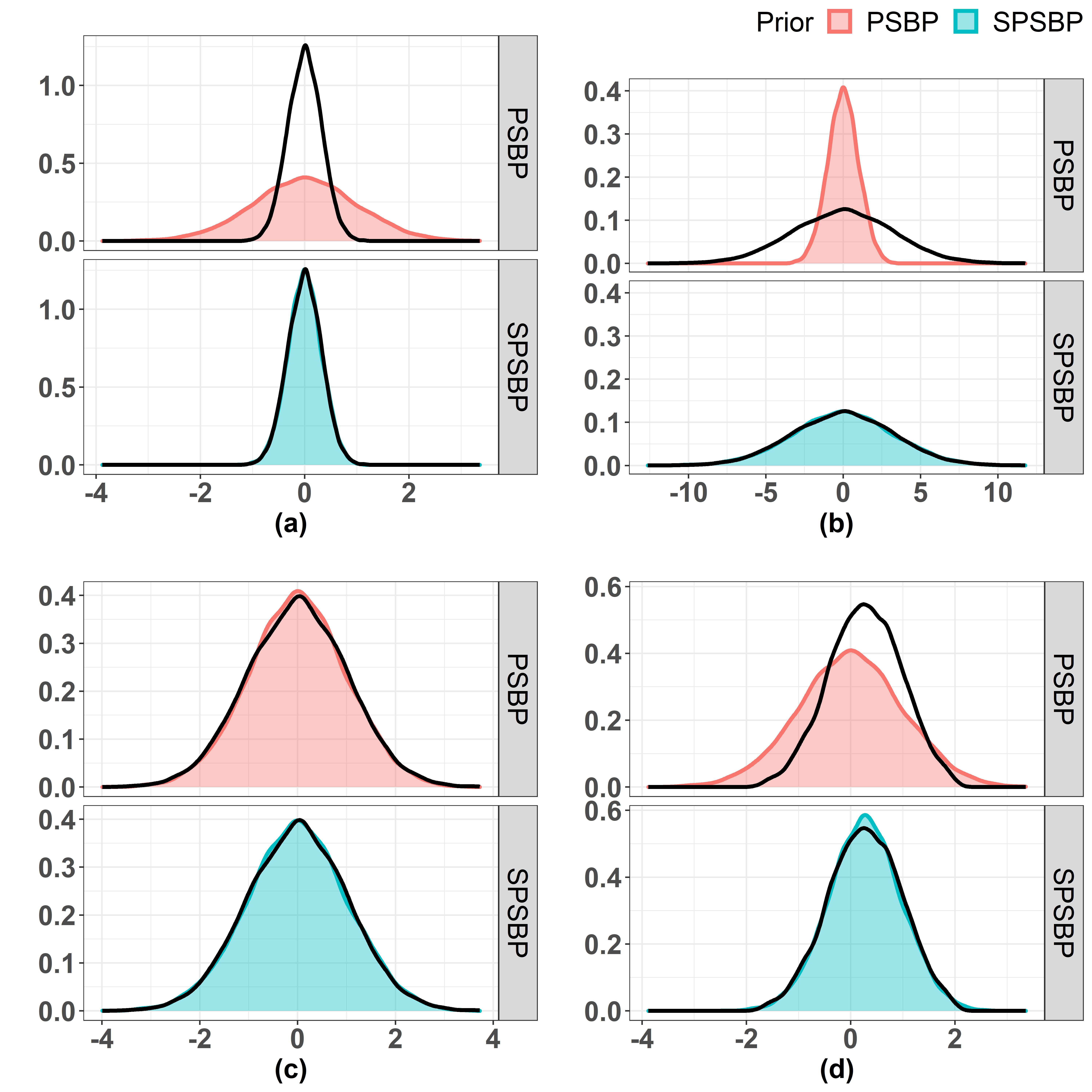
Figure 1: SPSBP versus PSPB prior: differences between with shrinkage effect and without shrinkage effect in assigning stick-breaking probabilities

Density plots for sample observations from $\psi(\bm{W})^{\prime}\alpha_{h}=\{\psi(\bm{w}_{i})^{\prime}\bm{\alpha}_{h},i=1,\ldots,N\}$ (black solid lines), a standard normal (PSBP prior), and a normal distribution with $\mu$ and $\sigma$ defined by 10 (SPSBP prior); $\psi(\bm{w}_{i})^{\prime}\bm{\alpha}_{h}$ is defined in 10; four $\bm{W}$ generation scenarios ($N=10,000$) are considered: ($a$) $\bm{W}\sim\mathcal{N}_{4}(\bm{0},0.1\cdot I_{4})$, ($b$) $\bm{W}\sim\mathcal{N}_{4}(\bm{0},10\cdot I_{4})$, ($c$) $\bm{W}\sim\mathcal{N}_{4}(\bm{0},I_{4})$, (d) same predictors generation scheme (RCT setting) as specified in the simulation studies section: $\bm{W}=\{A,X_{1},X_{2},X_{3}\},A\sim Binomial(10,000,0.5),X_{1}\sim N(0,1),X_{2}\sim Binomial(10,000,0.7),X_{3}\sim t(d.f.=5,ncp=0)$.

Another DSBP prior that can adjust for mixed-type predictors is the logit stick-breaking process (LSBP) prior introduced by Rigon and Durante, (2021). Assuming a LSBP prior, the $h^{th}$ stick-breaking probability is given by

$$v_{h}(\bm{w}_{i})=1/\{1-\exp(\bm{\psi}(\bm{w}_{i})^{\prime}\bm{\alpha}_{h})\},\quad\bm{\alpha}_{h}\sim\mathcal{N}_{R}(\bm{\mu},\bm{\Sigma}),\ h\in\{1,\ldots,L-1\}$$

Section 2.3 A Bayesian Non-parametric Inference Framework

Section 2.3.1 Subject-Level and Group-Level Estimands and Estimators

In Section 2.1, we provided a general definition of RMST as the expected survival time of time-to-event $T$ restricted to certain time point $[0,\tau]$. Conditional on the predictor matrix $\bm{W}$ and a fixed time point $\tau$, a conditional RMST function can be defined as

$$RMST_{\bm{\theta}}(t=\tau\;|\;\bm{W})=\int_{0}^{\tau}S_{\bm{\theta}}(t\;|\;\bm{W})\;dt,$$ (11)

which relates to the (marginal) RMST function by

$$RMST(t=\tau)=E_{\bm{W}}\big{[}RMST(t=\tau\;|\;\bm{W})\big{]}=\int_{-\infty}^{\infty}\int_{0}^{\tau}S_{\bm{\theta}}(t\;|\;\bm{W})f_{\bm{W}}(\bm{w})\;dtd\bm{W}$$ (12)

Tian et al., (2014) studied a class of frequentist regression models for estimating the conditional RMST given “baseline” covariate. In this section, we develop nonparametric Bayes conditional RMST inference, Let the observed $i^{th}$ time-to-event be $(Y_{i},\delta_{i})$ where $Y_{i}=\text{min}(T_{i},C_{i})$, $\delta_{i}=I(T_{i}\leq C_{i})$ and $C_{i}$ is the censoring variable including a maximum follow-up time of $\tau_{c}$. Also, $\bm{W}_{i}=(A_{i},\bm{X}_{i})$ where $\bm{X}_{i}$ is a vector of time-fixed covariate and $A_{i}$ is binary treatment group indicator. With a slight abuse of notation, let $\bm{\theta}$ denote the combined parameter vector of both the stick-breaking process prior and the kernel density. The posterior mean conditional RMST function for the $i^{th}$ subject is

$$\widehat{RMST}(t=\tau\;|\;\bm{w}_{i})=E_{\bm{\theta}}\left[\int_{0}^{\tau}S_{\bm{\theta}}(s\;|\;\bm{w}_{i})\;ds\;\;|\bm{Y},\bm{\delta}\right]$$ (13)

which can be estimated based on Markov chain samples $\{\bm{\theta}_{1},\ldots,\bm{\theta}_{L}\}$ and based on our model constructions in (1–7) as

$$\widehat{RMST}(t=\tau\;|\;\bm{w}_{i})=E_{\bm{\theta}}\Bigg{[}\sum_{h=1}^{L}\Big{[}\pi_{h}\big{(}\bm{\psi}_{1}(\bm{w}_{i})^{\prime}\bm{\alpha}_{h}\big{)}\int_{0}^{\tau}\int_{t}^{\infty}K\big{(}s\;|\;\bm{\psi}_{2}(\bm{w}_{i})^{\prime}\bm{\beta}_{h},\bm{\omega}_{h}\big{)}\;dsdt\Big{]}\Bigg{]}$$ (14)

where $1\leq L\leq\infty$, $\bm{\theta}=\{\bm{\alpha},\bm{\beta},\bm{\omega}\}$. Here we distinguish the linear transformation function ($\psi_{1}(\cdot)$) applied in the stick-breaking probabilities from the one ($\psi_{2}(\cdot)$) applied in the kernel density with different subscripts. Consequently, a $100(1-\alpha)\%$ credible interval (CI) for $RMST$ is $[\widehat{RMST}^{(\alpha/2)},\widehat{RMST}^{(1-\alpha/2)}]$ where $\widehat{RMST}^{(\alpha/2)}$ and $\widehat{RMST}^{(1-\alpha/2)}$ are calculated as the $(\alpha/2)$th and $(1-\alpha/2)$th quantiles of the posterior distribution of $RMST$.

Chen and Tsiatis, (2001) defined an average (marginal causal) treatment effect (ATE) in terms of the average group differential RMSTD under the counter-factual framework (Morgan and Winship,, 2015) by, that is,

$$\begin{split}\Delta&=RMST_{A_{1}}(t=\tau)-RMST_{A_{0}}(t=\tau)\\ &=\int_{0}^{\tau}E_{\bm{X}}\Big{[}S_{\bm{\theta}}(t\;|\;A=1,\bm{X})\Big{]}-E_{\bm{X}}\Big{[}S_{\bm{\theta}}(t\;|\;A=0,\bm{X})\Big{]}\;dt\end{split}$$ (15)

We define marginal Bayesian estimators of the causal estimand $\Delta$ defined in (15) using the empirical distribution of $\bm{X}$ as a nonparametric estimator of $f_{\bm{X}}(\bm{x})$

$$\begin{split}\widehat{\Delta}&=\frac{1}{N}\sum_{i=1}^{N}E_{\bm{\theta}}\left[\int_{0}^{\tau}S_{\bm{\theta}}(t\;|\;A=1,\bm{X}_{i}=\bm{x}_{i})-S_{\bm{\theta}}(t\;|\;A=0,\bm{X}_{i}=\bm{x}_{i})\;dt\right]\end{split}$$ (16)

Note that (27) does not adjust for potential confounding by censoring given our assumption that censoring is noninformative conditional on the covariate and treatment assignment, and that probability of censoring is positive. Given the constructions described in (1–7), we obtain

$$\begin{split}\widehat{\Delta}&=\frac{1}{N}\sum_{i=1}^{N}E_{\bm{\theta}}\left[\int_{0}^{\tau}S_{\bm{\theta}}(t\;|\;A=1,\bm{X}_{i}=\bm{x}_{i})-S_{\bm{\theta}}(t\;|\;A=0,\bm{X}_{i}=\bm{x}_{i})\;dt\right]\\ &=\frac{1}{N}\sum_{i=1}^{N}E_{\bm{\theta}}\Bigg{[}\sum_{h=1}^{L}\Big{[}\pi_{h}\big{(}\bm{\psi}_{A1,1}(\bm{w}_{i})^{\prime}\bm{\alpha}_{h}\big{)}\int_{0}^{\tau}\int_{t}^{\infty}K\big{(}s\;|\;\bm{\psi}_{A1,2}(\bm{w}_{i})^{\prime}\bm{\beta}_{h},\bm{\omega}_{h}\big{)}\;dsdt\\ &-\pi_{h}\big{(}\bm{\psi}_{A0,1}(\bm{w}_{i})^{\prime}\bm{\alpha}_{h}\big{)}\int_{0}^{\tau}\int_{t}^{\infty}K\big{(}s\;|\;\bm{\psi}_{A0,2}(\bm{w}_{i})^{\prime}\bm{\beta}_{h},\bm{\omega}_{h}\big{)}\;dsdt\Big{]}\Bigg{]}\end{split}$$ (17)

where $1\leq L\leq\infty$, $\bm{\theta}=\{\bm{\alpha},\bm{\beta},\bm{\omega}\}$, and $\bm{\psi}_{\cdot,\cdot}(\cdot)^{\prime}$ is a linear transformation function. Consequently, a $100(1-\alpha)\%$-level credible interval (CI) for $\Delta$ is given by $[\widehat{\Delta}^{(\alpha/2)},\widehat{\Delta}^{(1-\alpha/2)}]$ where $\widehat{\Delta}^{(\alpha/2)}$ and $\widehat{\Delta}^{(1-\alpha/2)}$ are calculated as the $(\alpha/2)$th and $(1-\alpha/2)$th quantiles of the posterior distribution of $\Delta$. The closed form equations of (14) assuming a Weibull and gamma kernel density, respectively, are shown in the appendix.

Section 2.4 Prior Specifications for Posterior Sampling of Proposed Approaches

Given sample observations $\big{\{}o_{i}=\big{(}y_{i},\bm{w}_{i}=(a_{i},\bm{x}_{i}),\delta_{i}\big{)}:i=1,\ldots,N\big{\}}$, we specify the likelihood and priors of the DSBP prior mixture models with covariates dependence on both the mixing probabilities and kernel densities in a hierarchical representation. For the $h^{th}$ cluster,

$$\begin{split}&y_{i}\ |\ \bm{\beta}_{i,h},\omega_{h}\stackrel{{\scriptstyle i.i.d.}}{{\sim}}K\big{(}y_{i}\;|\;exp\big{\{}\bm{\psi}(\bm{w}_{i})^{\prime}\bm{\beta}_{i,h}\big{\}},\omega_{h}\big{)},\quad i=1,\ldots,N\\ &v_{h}(\bm{w}_{i})=g(\bm{\psi}(\bm{w}_{i})^{\prime}\alpha_{h}),\;\pi_{1}(\bm{w}_{i})=v_{1}(\bm{w}_{i})\\ &\pi_{h}(\bm{w}_{i})=\big{(}1-v_{1}(\bm{w}_{i})\big{)}\big{(}1-v_{2}(\bm{w}_{i})\big{)}\ldots\big{(}1-v_{h-1}(\bm{w}_{i})\big{)}v_{h}(\bm{w}_{i}),\quad h\in\{2,\ldots,L-1\}\\ &\bm{\alpha}_{h}=\{\alpha_{h,A},\alpha_{h,1},\ldots,\alpha_{h,R}\}\sim\mathcal{N}_{R+1}(\bm{\mu}_{\alpha},\bm{\Sigma}_{\alpha}),\quad h\in\{1,\ldots,L-1\}\\ &\bm{\beta}_{h}=\{\beta_{h,A},\beta_{h,1},\ldots,\beta_{h,R}\}\sim\mathcal{N}_{R+1}(\bm{\mu}_{\beta},\bm{\Sigma}_{\beta}),\quad h\in\{1,\ldots,L\}\\ &\omega_{h}\sim unif(c_{low},c_{up}),\quad h\in\{1,\ldots,L\}\end{split}$$ (18)

where $(\bm{\mu}_{\alpha},\bm{\Sigma}_{\alpha},\bm{\mu}_{\beta},\bm{\Sigma}_{\beta},c_{low},c_{up})$ are constants, and $g(\cdot)$ can be a standard probit (regression) model, a shrinkage probit model (9), or an inverse logit (regression) model. We can choose $K(y_{i}\;|\;\cdot)$ to be either a Weibull kernel density (scale$=exp\big{\{}\bm{\psi}(\bm{w}_{i})^{\prime}\bm{\beta}_{ih}\big{\}}$, shape$=\omega_{h}$) or a gamma kernel density (rate$=exp\big{\{}\bm{\psi}(\bm{w}_{i})^{\prime}\bm{\beta}_{ih}\big{\}}$, shape$=\omega_{h}$) whose support is on $\mathbb{R}^{+}$. We reparameterize $\bm{\psi}(\bm{w}_{i})^{\prime}\bm{\beta}_{ih}$ on an exponential scale in order to select priors with support on $\mathbb{R}^{+}$. The $\bm{\alpha}$ matrix is of dimension $N\times(L-1)$ since $\pi(\bm{w})$ has $L-1$ degrees of freedom ($\pi_{L}(\bm{w})=1-\sum_{h=1}^{L-1}\pi_{h}(\bm{w})$). Let $\mathcal{Q}(\cdot)$ denote the log joint density function, and let $h(\cdot)$ and $H(\cdot)$ denote the density and cumulative distribution function of the censoring r.v., respectively. Assuming a non-informative right censoring mechanism,

$$\begin{split}&\mathcal{Q}\big{(}\bm{\theta}=(\bm{\alpha},\bm{\beta},\bm{\omega}),\bm{o}\big{)}=\prod_{i=1}^{N}\Big{\{}\big{[}f_{\bm{\theta}}(y_{i})\big{(}1-H(y_{i})\big{)}\big{]}^{\delta_{i}}\big{[}S_{\bm{\theta}}(y_{i})h(y_{i})\big{]}^{(1-\delta_{i})}\Big{\}}\\ &\propto\prod_{i=1}^{N}\sum_{j=1}^{L}\Big{\{}v_{j}(\bm{w}_{i})\prod_{l<j}\big{[}1-v_{l}(\bm{w}_{i})\big{]}\Big{\}}\cdot\Big{[}K\big{(}y_{i}\;|\;exp\big{\{}\bm{\psi}(\bm{w}_{i})^{\prime}\bm{\beta}_{i,j}\big{\}},\omega_{j}\big{)}\Big{]}^{\delta_{i}}\\ &\cdot\Big{[}\int_{t}^{\infty}K\big{(}y_{i}\;|\;exp\big{\{}\bm{\psi}(\bm{w}_{i})^{\prime}\bm{\beta}_{i,j}\big{\}},\omega_{j}\big{)}\Big{]}^{(1-\delta_{i})}\propto\prod_{i=1}^{N}\sum_{j=1}^{L}\Big{\{}g(\bm{\psi}(\bm{w}_{i})^{\prime}\bm{\alpha}_{i,j})\prod_{l<j}\big{[}1-g(\bm{\psi}(\bm{w}_{i})^{\prime}\bm{\alpha}_{i,j})\big{]}\Big{\}}\\ &\cdot\Big{[}K\big{(}y_{i}\;|\;exp\big{\{}\bm{\psi}(\bm{w}_{i})^{\prime}\bm{\beta}_{i,j}\big{\}},\omega_{j}\big{)}\Big{]}^{\delta_{i}}\cdot\Big{[}\int_{t}^{\infty}K\big{(}y_{i}\;|\;exp\big{\{}\bm{\psi}(\bm{w}_{i})^{\prime}\bm{\beta}_{i,j}\big{\}},\omega_{j}\big{)}\Big{]}^{(1-\delta_{i})}\end{split}$$

where $\bm{\alpha}=\{\bm{\alpha}_{i,j}\;|\;i=1,\ldots,N,j=1,\ldots,L-1\};\;\bm{\alpha}_{i,j}=\{\bm{\alpha}_{i,j,1},\ldots,\bm{\alpha}_{i,j,R}\}$, $\bm{\beta}=\{\bm{\beta}_{i,j}\;|\;i=1,\ldots,N,j=1,\ldots,L\};\;\bm{\beta}_{i,j}=\{\bm{\beta}_{i,j,1},\ldots,\bm{\beta}_{i,j,R}\}$, $\bm{\omega}=\{\omega_{1},\ldots,\omega_{L}\}$, $\bm{o}=\{\bm{o}_{1},\ldots,\bm{o}_{N}\};\;o_{i}=\{y_{i},\delta_{i},\bm{w}_{i}\}$.

Section 3 Simulation Studies

Section 3.1 Survival and Censoring Time Data Generation Models

We consider two data generation settings: ($i$) randomized controlled trial (RCT) with a balanced design; ($ii$) observational study where treatment assignments are confounded by observed covariates. We focus on simulating time-to-event data using various data generative models at different sample size levels, e.g., $N=\{200,500,1,000\}$. We consider a non-informative right-censoring mechanism with two components: ($i$) all patients are subject to random censoring/drop-out after enrollment; ($ii$) all patients who don’t experience an event are censored after a maximum follow-up time. Hence, we assign a time-to-censoring random variable with an exponential distribution $C\sim exp(rate=\lambda_{C}=0.05)$ and censor all observations beyond a maximum follow-up time of $\tau_{c}=10.5$ years. We also incorporate a random recruitment mechanism ($2$-year period) following a uniform distribution of ($0,2$). We independently generate three covariates of mixed-type ($2$ continuous and $1$ discrete): $X_{1}\sim\mathcal{N}(0,1)$, $X_{2}\sim Binomial(N,p)$, and $X_{3}\sim t(d.f.=5,ncp=0)$. Therefore, the observed data is of structure: $o_{i}=(a_{i},x_{i,1},x_{i,2},x_{i,3},y_{i},\delta_{i}),\ \text{for}\ i=1,\ldots,N;\;\bm{o}=\{o_{1},\ldots,o_{N}\}$ where $y_{i}=min(c_{i},t_{i},\tau_{c})$ and $\delta_{i}=\mbox{\boldmath$1$}\{t_{i}\leq c_{i}\}$. For notational convenience, we denote the tuple of covariates and treatment assignment for the $i^{th}$ patient by $w_{i}=(a_{i},x_{i})$. For the RCT setting, we randomly assign patients, with equal probability of $50\%$ ($A\sim Binomial(N,p=0.5)$), to one of the two treatment groups: a test and a control group denoted by $A_{1}$ and $A_{0}$, respectively. For the observational study setting, we specify treatment assignment probabilities as a linear combination of covariates values under a logit transformation: $logit(p_{i})=\bm{x}_{i}^{T}\bm{\beta}_{i}$ where $\bm{x}_{i}=\{x_{i,1},x_{i,2},x_{i,3}\}$ and $\bm{\beta}=\{\beta_{1}=1,\beta_{2}=1,\beta_{3}=1\}$ for $i=1,\ldots,N$ such that $A_{i}\sim Binom(N,p=\bm{x}_{i}^{\prime}\bm{\beta})$. Under the Weibull survival time generation model, the data generating model for survival time $T$ is a Weibull distribution with baseline shape parameter $\gamma_{0}$, baseline scale parameter $\lambda_{0}$ and multiplicative covariates effects. For the $i^{th}$ patient, its survival function is specified as:

$$S_{i}(t)=exp\{-\lambda_{0}(t^{\gamma_{0}})exp(\bm{w}_{i}^{\prime}\bm{\beta}_{Weibull})\}$$ (19)

where $\bm{w}_{i}=\{a_{i},x_{i,1},x_{i,2},x_{i,3}\}$, $\bm{\beta}_{Weibull}=\{\beta_{a}=-2.5,\beta_{x1}=1.5,\beta_{x2}=2.5,\beta_{x3}=1.5\}$, $\lambda_{0}=1.5$, and $\gamma_{0}=1.5$. The true RMST value for the $i^{th}$ patient is evaluated by integrating (19) from $t=0$ to $\tau$ given the patient’s covariates values and coefficients of covariates effect ($\bm{\beta}_{Weibull}$). Under the lognormal survival time generation model, the survival time $T$ is assigned a lognormal distribution with a fixed standard deviation $(\sigma=1)$ and mean parameter that is a linear combination of covariates $(\mu=\bm{w}^{\prime}\bm{\beta})$. For the $i$th subject,

$$t_{i}\stackrel{{\scriptstyle i.i.d.}}{{\sim}}Lognormal\;\big{(}log(\mu_{i})=\bm{w}_{i}^{\prime}\bm{\beta}_{lognormal},\ log(\sigma_{i})=1\big{)}$$ (20)

where $\bm{w}_{i}=\{a_{i},x_{i,1},x_{i,2},x_{i,3}\}$, and $\bm{\beta}_{lognormal}$ controls covariates’ effect on survival. We assign $\bm{\beta}^{1}_{lognormal}=\{\beta_{a}=2.5,\beta_{x1}=1.5,\beta_{x2}=2.5,\beta_{x3}=1.5\}$ for a positive treatment effect (default setting), $\beta_{x1}=-1.5$, and $\beta_{x1}=0$ for a negative and null treatment effect, respectively. The true RMST value for the $i^{th}$ patient is evaluated by $\int_{0}^{\tau}1-\Phi\big{(}(t_{i}-\mu_{i})\big{)}dt_{i}$ given the patient’s covariates values and coefficients of covariates effect ($\bm{\beta}_{lognormal}$). Additionally, we consider a two-component Weibull mixture survival time generation model, which allows for more flexible baseline hazard functions. The two-component mixture Weibull distributions are additive on the survival scale, with a mixing proportion parameter $\rho$, i.e. $S(t)=\rho S_{1}(t)+(1-\rho)S_{2}(t)$. The survival function for the $i^{th}$ patient is defined as

$$\begin{split}S_{i}(t)=\big{(}\rho\cdot e^{-\lambda_{0}^{1}(t^{\gamma_{0}^{1}})}+(1-\rho)\cdot e^{-\lambda_{0}^{2}(t^{\gamma_{0}^{2}})}\big{)}^{exp\{\bm{w}_{i}^{\prime}\bm{\beta}_{2Weibull}\}}\end{split}$$ (21)

where $\rho$ denotes the mixture proportion; ($\lambda_{0}^{1},\gamma_{0}^{1}$), ($\lambda_{0}^{2},\gamma_{0}^{2}$) denote the baseline scale and shape parameters for the two mixture distributions; $\bm{w}_{i}=\{a_{i},x_{i,1},\ldots,x_{i,R}\}$ denotes observed treatment assignment and covariates for the $i^{th}$ subject; $\bm{\beta}_{2Weibull}$ denotes the coefficients of covariates effect. The true RMST value for the $i^{th}$ patient is evaluated by integrating 21 from $t=0$ to $\tau$ given $(\bm{w}_{i},\bm{\beta}_{2Weibull})$ where the coefficients $\bm{\beta}_{2Weibull}$ are set at the same numerical values as $\bm{\beta}_{Weibull}$ and $\bm{\beta}^{2}_{lognormal}$.

Section 3.2 Simulation Scenarios

For a comprehensive evaluation of our inferential tools, we consider a total of $6$ data generation scenarios: {$3$ data generation models: Weibull, lognormal, and two-components Weibull mixture}$\times${$2$ study settings: randomized controlled trial and observational study}. The lognormal model has two extra covariates settings: negative and null treatment effects in addition to the default positive treatment effect setting shared by the Weibull and two-component Weibull mixture models. We evaluate performance of the proposed BNP estimators of RMST, and compare with two frequentist methods: ($i$) Tian et al., (2014)’s direct (RMST) regression method; ($ii$) Ambrogi et al., (2022)’s pseudo-values method. We make evaluations in terms of bias, root mean square error (RMSE), and coverage probability (CP). We also evaluate Bayesian models’ performance under different choices of DSBP priors and kernel densities. For each simulation scenario, we randomly generate and fix a sample of covariates ($\bm{W}$) at a given sample size. Then for each simulation replication, we randomly generate a sample of outcomes ($\bm{Y},\bm{\delta}$) given $\bm{W}$ and make inferences given observed data $\bm{O}=(\bm{W},\bm{Y},\bm{\delta})$. In an oncology study setting, $5$ year is usually considered a mile-stone for treatment evaluation. Hence for fixed-time analysis, our simulation studies evaluate RMST estimations at $\tau=5$ years. Besides, we conduct RMST curve estimations on a grid of time points. For prior specifications, we set $\big{(}\bm{\mu}_{\alpha}=\bm{0},\bm{\Sigma}_{\alpha}=400\cdot I_{4},\bm{\mu}_{\beta}=\bm{0},\bm{\Sigma}_{\beta}=400\cdot I_{4},c_{low}=\{0.01,0.1\},c_{up}=\{10,15\}\big{)}$ (LABEL:gSB-mix-mod-spec-1) such that $\bm{\alpha}$ and $\bm{\beta}$ each follows a four-dimensional Gaussian distribution with an independent covariance structure and equal standard deviation of $20$ for each predictor. We use a minimum burn-in iteration size of $2,000$ and a minimum posterior sampling iteration size of $1,000$ for all NUTS runs. Initial values are provided by Stan as a default setting.

Section 3.3 Simulation Results

Figure 2 shows estimation results on ATE by BNPDM models assuming a SPSBP prior and a PSBP prior, both with a Weibull kernel density, where survival data are generated by a lognormal model under a RCT setting. Dots and bars denote point estimates and credible intervals, respectively. A bar and a dot are colored red together if the credible interval covers the true/population ATE. Given a moderate sample size ($500$), biases (averaged over $100$ replications) of both models are near zero. However, credible intervals and RMSE estimated under the SPSBP prior are much tighter and smaller compared to those of the PSBP prior. Specifically, the average credible interval (CI) length of the SPSBP prior is less than half of that of the PSBP prior ($0.33/0.74\approx 0.45$). The (default) PSBP prior model give volatile estimates while the modified PSBP prior (SPSBP prior) model stabilize estimates and results in “shrinked” credible intervals in comparison.

Figure 2: Single time point analysis scenario 1: ATE point estimates with 95% credible intervals comparing SPSBP prior with PSBP prior (lognormal data generation model under a RCT setting; $\tau=5$)

(a) SPSBP prior-Weibull kernel: CP = 0.91, Average CI Length=0.33, bias = 0.05, RMSE = 0.1

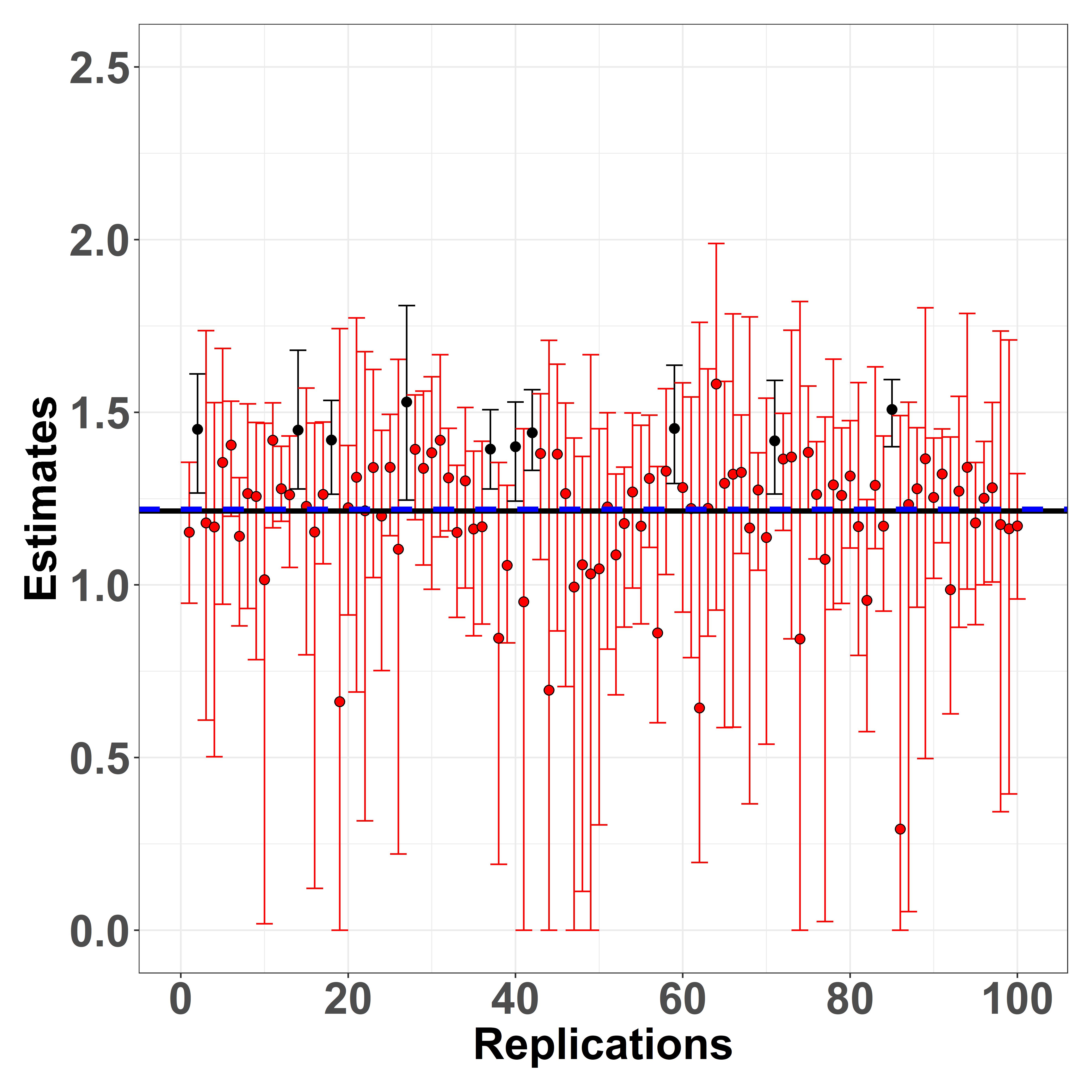
(b) PSBP prior-Weibull kernel: CP = 0.9, Average CI Length=0.74, bias = 0.01, RMSE = 0.2

CP denotes coverage probability; ACredIntL denotes average credible intervals’ length; sample size $N=500$; RMSTD evaluated at $\tau=5$ years; coefficients of predictor effects: $(\beta_{A}=2.5,\beta_{W_{1}}=1.5,\beta_{W_{2}}=2.5,\beta_{W_{3}}=1.3)$; black solid lines and blue dashed lines mark the true RMSTD value and average RMSTD point estimates, respectively.

Figure 3 shows results estimated by the LSBP prior and the LDDP prior models, both with a Weibull kernel density, under the same lognormal-RCT data generation setting. The LSBP and LDDP prior models result in higher biases and RMSEs, yet slightly smaller average CI length compared to the SPSBP prior (model). However, their CPs are very low ($52\%$ and $21\%$) compared to SPSBP prior and PSBP prior ($91\%$ and $90\%$) though the PSBP prior’s CP may be inflated due to its extra wide credible intervals.

Figure 3: Single time point analysis scenario 2: ATE point estimates with 95% credible intervals comparing LSBP prior with LDDP prior (lognormal data generation model under a RCT setting; $\tau=5$)

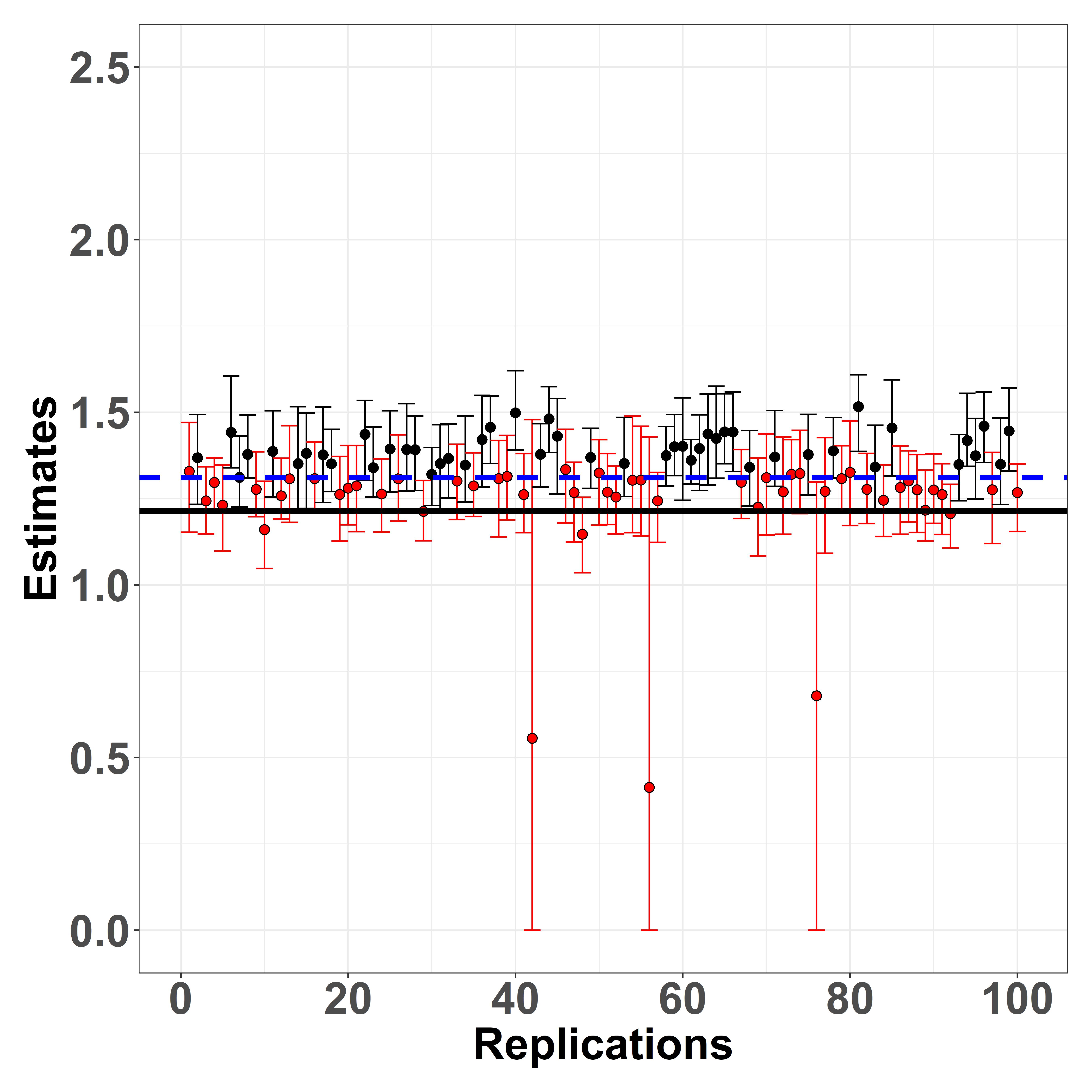
(a) LSBP prior-Weibull kernel: CP = 0.52, Average CI Length=0.26, bias=0.1, RMSE=0.18

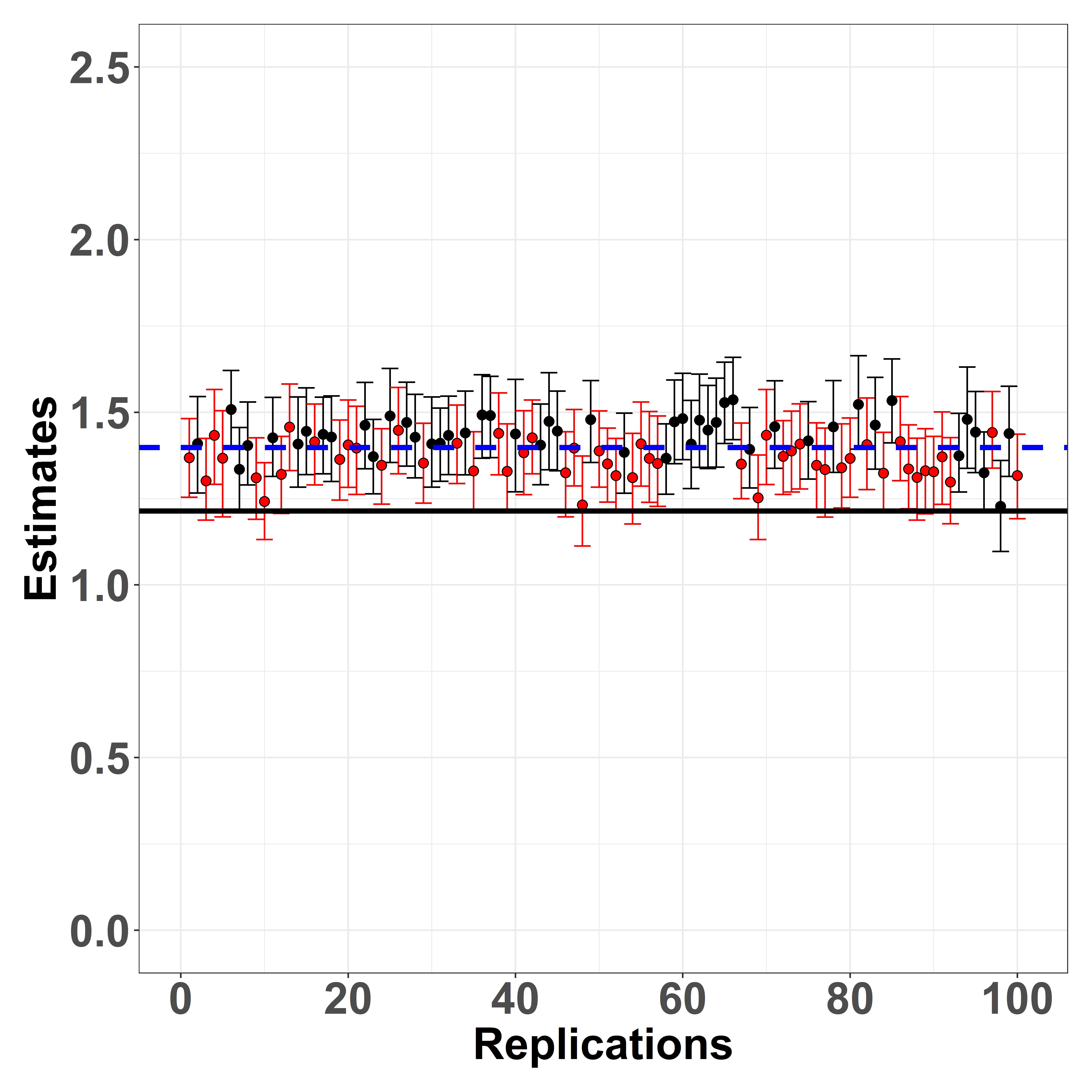
(b) LDDP prior-Weibull kernel: CP = 0.21, Average CI Length=0.24, bias=0.18, RMSE=0.2

CP denotes coverage probability; ACredIntL denotes average credible intervals’ length; sample size $N=500$; RMSTD evaluated at $\tau=5$ years; coefficients of predictor effects: $(\beta_{A}=2.5,\beta_{W_{1}}=1.5,\beta_{W_{2}}=2.5,\beta_{W_{3}}=1.3)$; black solid lines and blue dashed lines mark the true RMSTD value and average RMSTD point estimates, respectively.

Regarding subject-level RMST inference, all DSBP prior (SPSBP, PSBP, and LSBP) models have superior performance compared to their frequentist counterparts (Tian et al.,, 2014; Ambrogi et al.,, 2022) under the two-components Weibull mixture data generation model as shown in Figure F1–F5 (supplemental materials). Numerical results (for $\tau=5$; Figure F1–F2) in Table 1 show that, with a sample size of $500$, RMSE given by the SPSBP prior is less than half of that by Tian et al., (2014)’s method ($0.25$ compared to $0.57$). For subject-level CP, which is defined by the proportion of time the credible or confidence interval covers the true individual RMSTD value, the LSBP prior yields $0.88$. In comparison, CP by Tian et al., (2014) and Ambrogi et al., (2022) are both $0.48$. Furthermore, this higher CP is not achieved with increased interval width. On the contrary, the average credible interval length of the LSBP prior is $0.42$ compared to $0.75$ (average confidence interval length) given by the frequentists’ methods.

Table 1: SUBJECT-LEVEL RMST PREDICTIONS SCENARIO 1-A

Method	Bias	RMSE	Coverage Probability	Average Credible/ Confidence Interval Length
SPSBP-Weibull	0.08	0.25	0.556	0.3121
PSBP-Weibull	0.01	0.19	0.886	0.3830
LSBP-Weibull	0.04	0.21	0.880	0.4164
LDDP-Weibull	0.18	0.37	0.402	0.2239
Tian et al., (2014)	0.00	0.57	0.484	0.7477
Ambrogi et al., (2022)	0.00	0.57	0.484	0.7448

Restricted mean survival time is a function of restricted time, and estimating RMST at only a single time point $\tau$ does not tell the whole story of temporal survival relationship. Therefore, we expand the time horizon to evaluate the performance of BNPDM models for RMST inference on a grid of time points ($\tau$s). We calculate point estimates and point-wise credible intervals. On the other hand, given $\tau$ and posterior sample $\bm{\theta}$ drawn from $Pr(\bm{\theta}\;|\;\bm{Y},\bm{\delta},\bm{W})$, the RMST function is just a deterministic function of these quantities. Therefore, we can attain an entire RMST curve estimate with a single NUTS run. We estimated RMST curves under $100$ data replications and show their results in Figures F11–F20 (supplemental materials). The corresponding numerical results are summarized in Table 2.

Table 2: Subject-level RMSTD Curve Inference Results; Data generation model is a 2-components Weibull mixture model

$\bm{\tau}$	Average Absolute Bias					RMSE
	SPSBP Weibull	LSBP Weibull	LSBP Gamma	Tian et al. (2014)	Ambrogi et al. (2022)	SPSBP Weibull	LSBP Weibull	LSBP Gamma	Tian et al. (2014)	Ambrogi et al. (2022)
1	0.67	0.04	0.10	0.08	0.08	1.2	0.06	0.13	0.10	0.10
2	0.53	0.06	0.11	0.17	0.17	1.04	0.10	0.17	0.21	0.21
3	0.42	0.08	0.14	0.28	0.28	0.86	0.14	0.24	0.34	0.34
4	0.34	0.10	0.16	0.37	0.37	0.70	0.18	0.30	0.47	0.47
5	0.28	0.12	0.18	0.44	0.44	0.55	0.23	0.36	0.57	0.57
6	0.24	0.14	0.20	0.50	0.50	0.42	0.27	0.41	0.67	0.67
7	0.21	0.15	0.21	0.55	0.55	0.33	0.31	0.46	0.75	0.75
8	0.19	0.16	0.23	0.58	0.59	0.29	0.36	0.51	0.83	0.83
9	0.21	0.18	0.24	0.61	0.62	0.32	0.40	0.55	0.90	0.90
10	0.23	0.19	0.25	0.64	0.65	0.39	0.44	0.59	0.96	0.96

Section 4 Real Data Applications

The epidermal growth factor receptor (EGFR) has been proven to be a clinically meaningful target for monoclonal antibodies (mAbs) with efficacy established in treatment of metastatic colorectal cancer (mCRC) (Cunningham et al.,, 2004; Bokemeyer et al.,, 2009). Panitumumab (Pmab) is a (fully) human anti-EGFR that was approved as monotherapy for patients with chemotherapy-refractory mCRC (Giusti et al.,, 2007). A randomized phase III study was designed and conducted to evaluate the efficacy and safety of Pmab plus infusional fluorouracil, leucovorin, and oxaliplatin (FOLFOX4) versus FOLFOX4 alone as an initial treatment for mCRC in patients with previously untreated mCRC according to tumor KRAS status (Douillard et al.,, 2010). The presence of activating KRAS mutations was identified as a potent predictor of resistance to EGFR-directed antibodies (e.g., cetuximab and panitumumab) (Heinemann et al.,, 2009). In this real data application example we only focus on RMSTD inference among KRAS wild type (WT) patients for its clinical relevance.

This phase III study was designed as an open-label, randomized, phase III trial to compare the treatment effect of adding Pamb to FOLFOX4 in patients with WT KRAS tumors and also in patients with mutant (MT) KRAS tumors (Douillard et al.,, 2010). A primary analysis of log-rank tests, stratified by random assignment factors, were conducted on the progression-free survival (PFS) and overall survival (OS) endpoints among the WT KRAS and MT KRAS patient stratums (Douillard et al.,, 2010). A prespecified final analysis, which included OS, was later reported in (Douillard et al.,, 2014). We conduct a reanalysis of the selected study to estimate group differential treatment effect on the OS endpoint. The maximum observed event time is approximately $3.8$ years, and we evaluate RMSTD up to $3.5$ years. We include BMI and age as predictive covariates, which are both prognostic in mCRC (Lieu et al.,, 2014). With all incomplete records removed, the study population has a total number of $652$ observations. We apply BNPDM models with SPSBP and LSBP priors both assuming a Weibull and Gamma kernel densities. We obtained both point estimates and credible intervals from month $1$ to month $45$ with an increasing step size of $1$ month. We compare results under both BNPDM models with those given by Tian et al., (2014)’s method in Figure 4(g) and show a numerical summary in Table T1 (supplemental materials).

Figure 4: RMSTD curve estimation: real data analysis–comparing average treatment effect difference between FOLFOX4+Panitumumab versus FOLFOX 4 using PRIME (Douillard et al.,, 2010) data (unit: months, sample size: $N=1,092$)

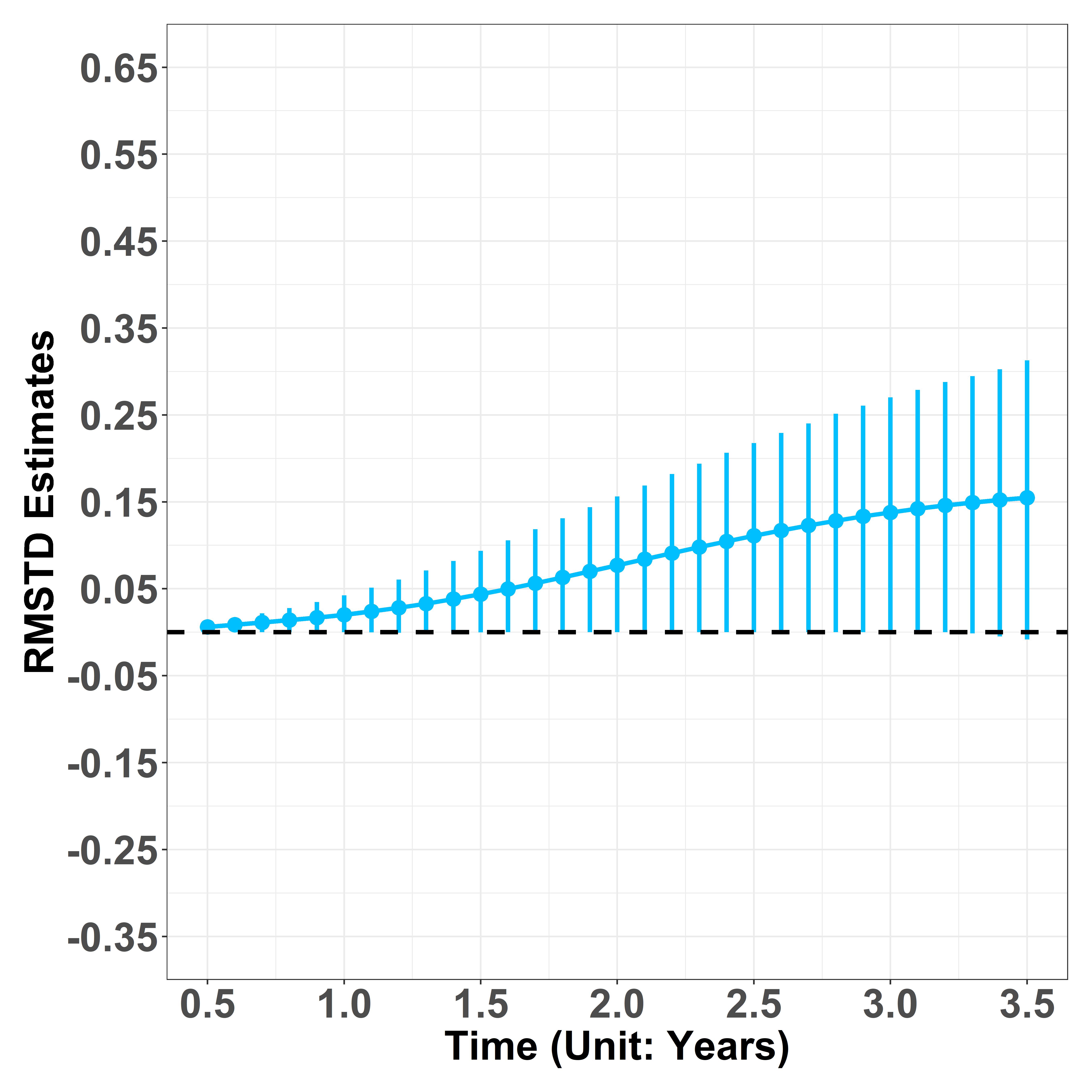
(a) LSBP-Weibull

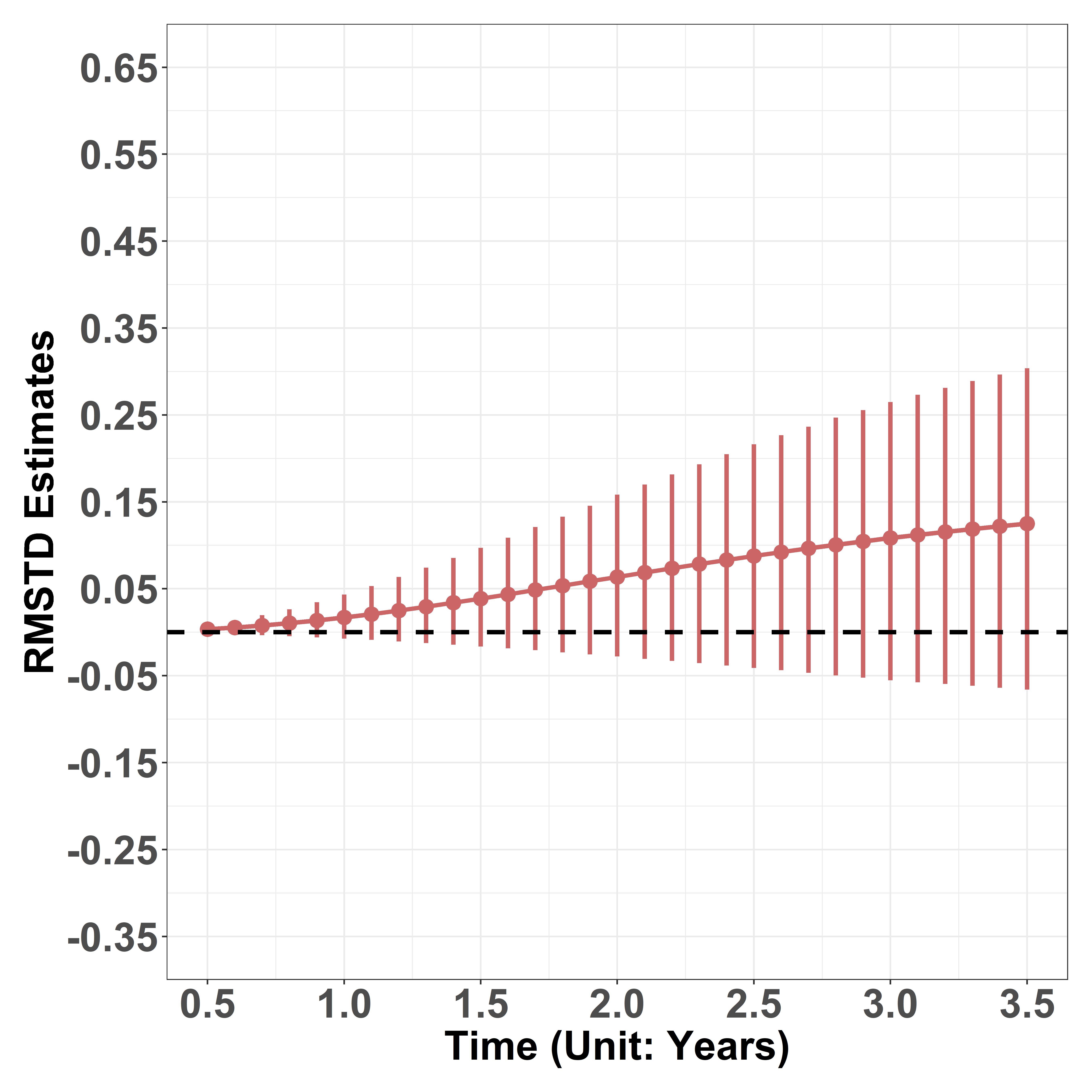
(b) SPSBP-Weibull

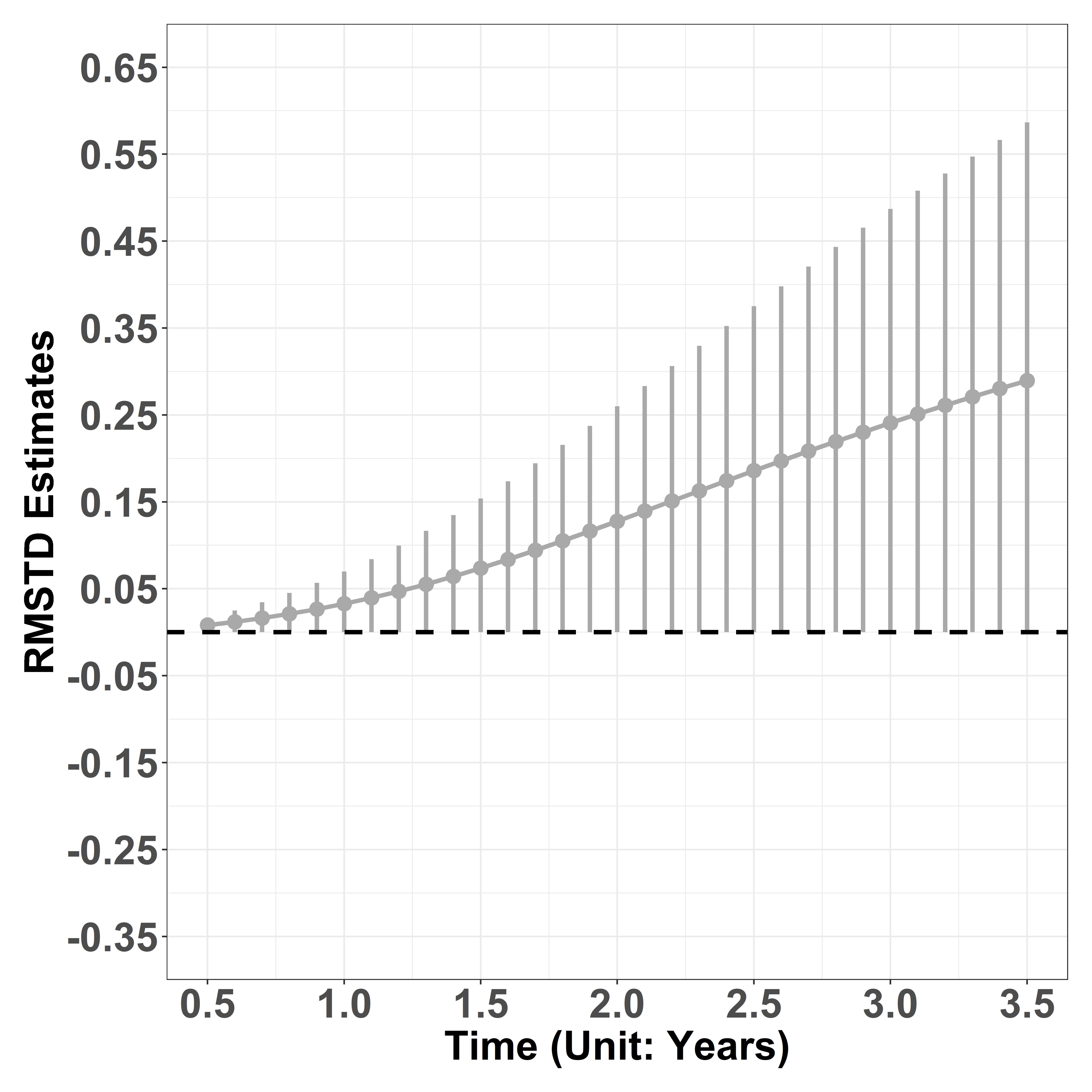
(c) PSBP-Weibull

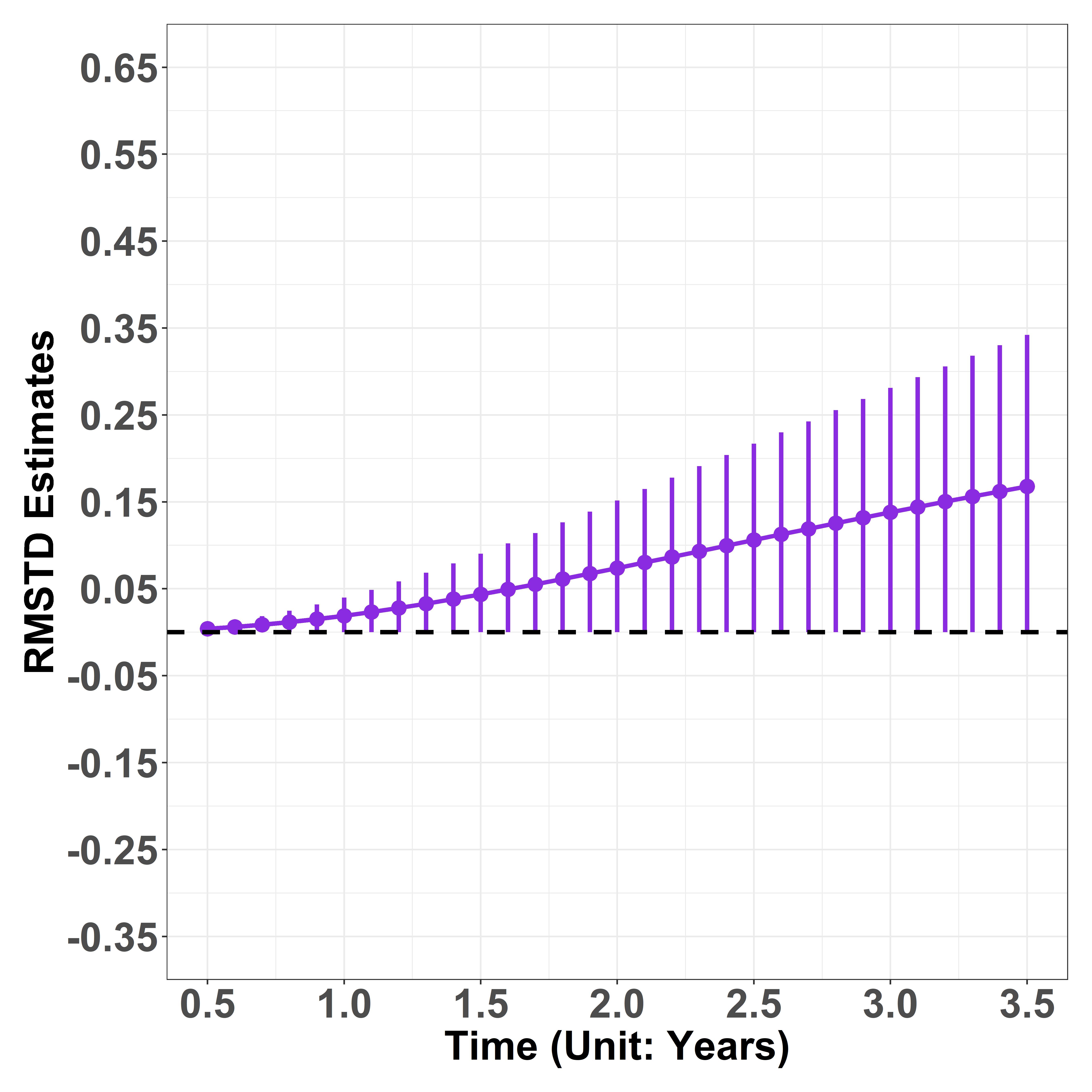
(d) LSBP-Gamma

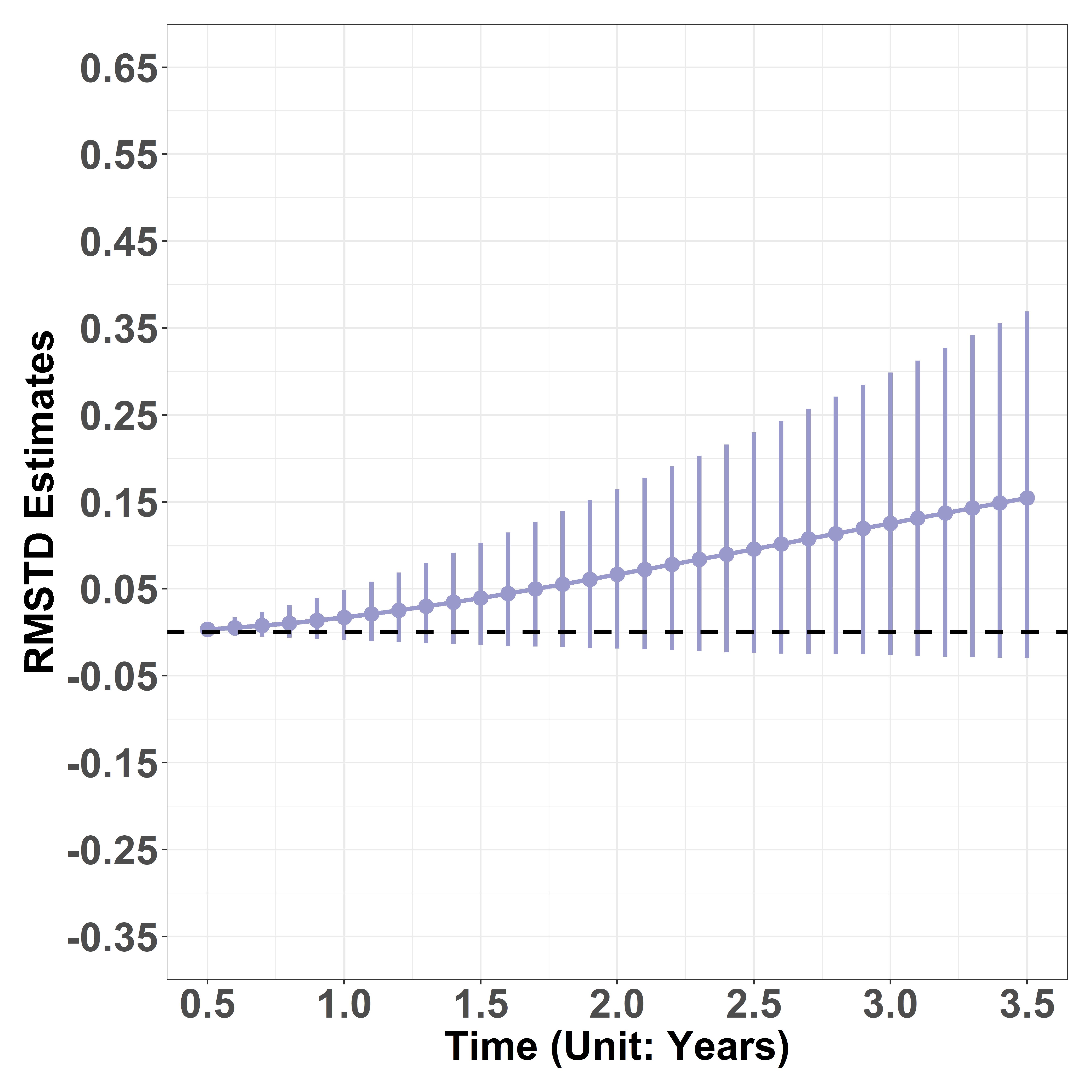
(e) SPSBP-Gamma

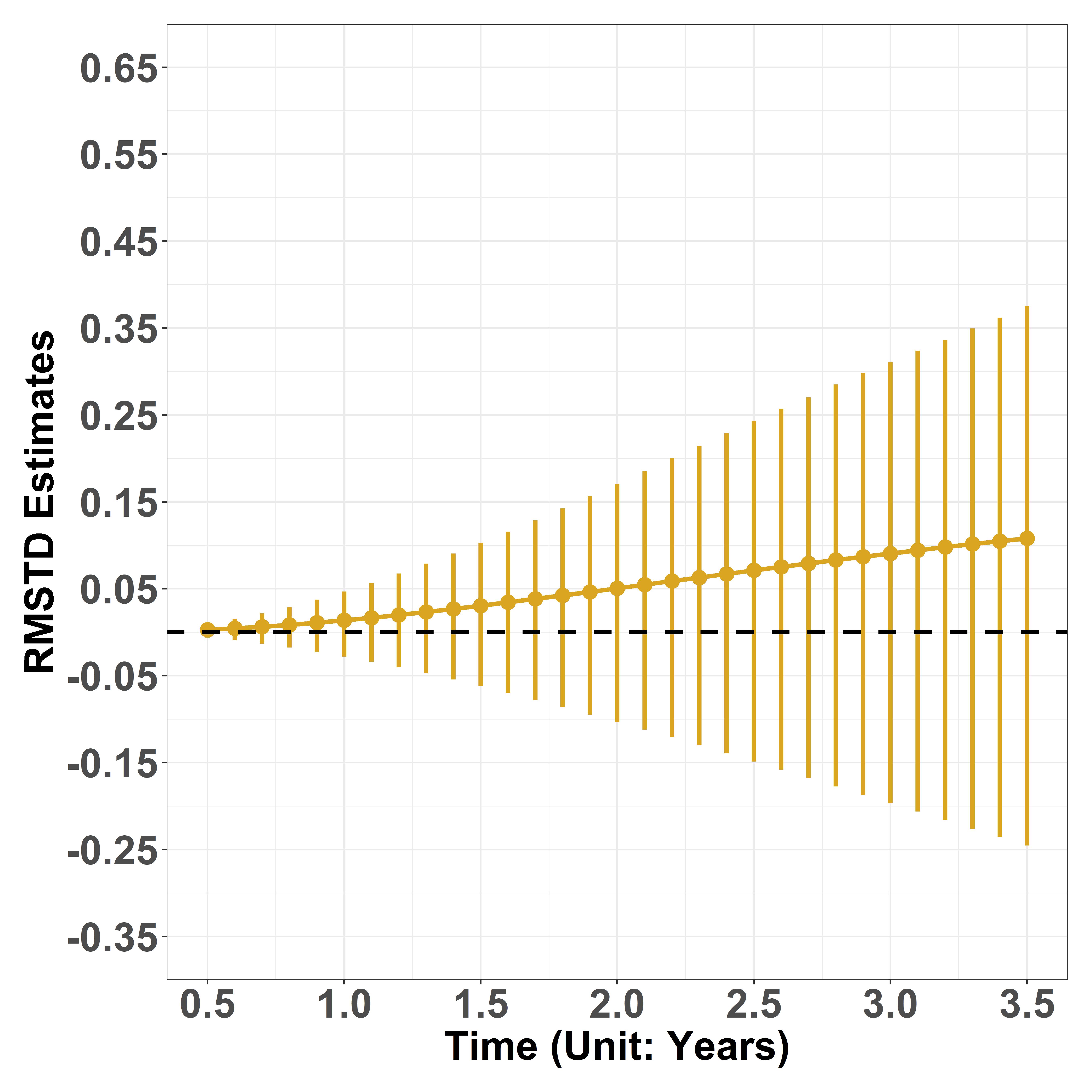
(f) PSBP-Gamma

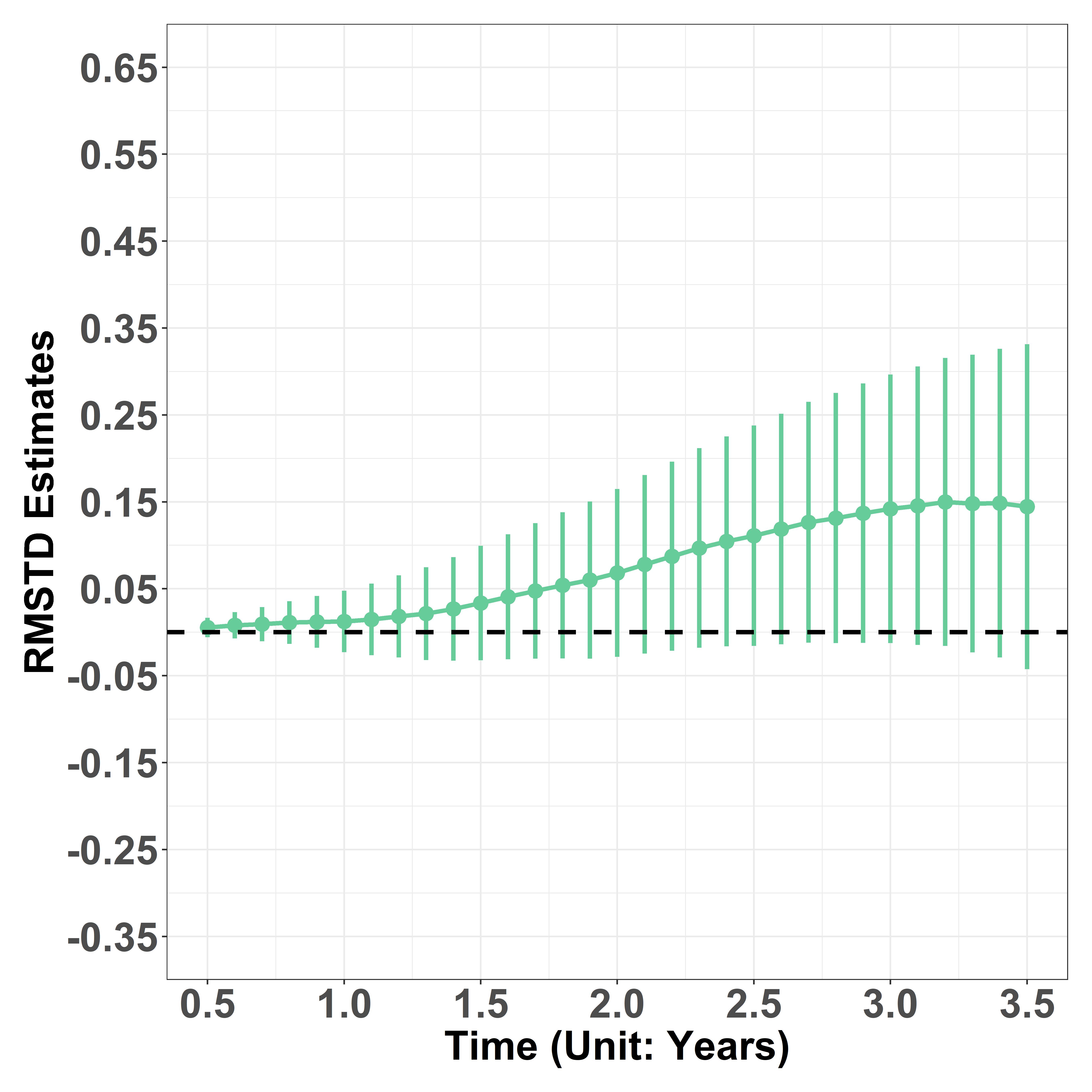
(g) Tian et al., (2014)

Section 5 Discussions

In this article, we constructed a BNP estimation framework for estimating treatment effect measured by both average group differential RMST and subject-level RMST. Zhang and Yin, (2022) proposed a BNP RMST estimator by putting mixture of Dirichlet process priors on the cumulative distribution function of the survival time random variable. Taking a different route, we treat the density of survival function hierarchically as a mixture of kernel densities where the mixtures have a (dependent) stick-breaking process prior. Our modeling approach is analogous to that of a dependent DP mixture (DDPM) model but with a more flexible stick-breaking probability assignment mechanism. A major advantage of our approach is to enable adjustments of mixed-type covariates/predictors. While many works on modeling spatial data focus on dependent structures that adjust for continuous covariates (Reich et al.,, 2007; Ren et al.,, 2011; Diana et al.,, 2020), mixed-type covariates are more often seen in clinical settings. When the data generation model is a function of covariates, both group-level and subject-level RMST inference could be less efficient or inconsistent, without properly adjusting for the observed covariates.

We proposed a novel dependent stick-breaking process prior: the SPSBP (shrinkage probit stick-breaking process) prior, which is inspired by Rodriguez and Dunson, (2011)’s (dependent) PSBP (probit stick-breaking process) prior. The SPSBP prior results in less variable estimates (e.g., narrower credible intervals) given a small or moderate sample size compared to the PSBP prior. This shrinkage effect is achieved through a more efficient stick-breaking probability assignment process that utilizes the sample first and second (central) moments of the empirical density function of the linearly transformed covariates. However, since the level of shrinking is controlled by sample variance and inversely proportional to the observed sample size, having a huge sample size could results in assigning the entire unit length towards the first few sticks, which results in a less discrete realization of the stick-breaking process. Fortunately, we did not experience such issue when modeling data up to $2,000$ observations and $10$ clusters. In fact, we found out through simulation studies that modeling with a smaller cluster size ($3$ or $5$) often result in better performance, compared to using say $10$ clusters, under a sample size between $200$ and $2,000$.

Our simulation studies show decent performance by BNPDM models on group-level RMSTD inference giving ignorable biases and CPs up to $90\%$ for a $95\%$ nominal under Weibull and lognormal data generation models (RCT setting). In comparison, the two frequentist methods (Tian et al.,, 2014; Ambrogi et al.,, 2022) give consistent point estimates and CPs that attain the nominal level of $95\%$ under the same data generation settings (Weibull-RCT or lognormal-RCT). Credible sets of infinite-dimensional Bayesian models are not automatically frequentist confidence sets, and it is not automatically true that they contain the truth with the probability at least the credible level (Szabó et al.,, 2015). The less efficiency of certain BNP models is well studied in the literature. For example, see (Cox,, 1993; Diaconis and Freedman,, 1997). However, we found that BNPDM models’ subject-level RMST prediction results are better than those of frequentist methods (Tian et al.,, 2014; Ambrogi et al.,, 2022) when the underlying data generation model is a two-component mixture of Weibulls. Besides, we found our BNPDM models have more robust performances against cases where treatment assignment is confounded by observed covariates compared to Tian et al., (2014); Ambrogi et al., (2022)’s methods.

Appendix

Assuming a Weibull kernel density (scale=$\bm{\psi}(\bm{W})^{\prime}\bm{\beta}$, shape=$\omega$), (14) has a closed form

$$\begin{split}&\widehat{RMST}(t=\tau\;|\;\bm{w}_{i})=E_{\bm{\theta}}\Bigg{[}\sum_{h=1}^{L}\Bigg{\{}\pi_{h}\big{(}\bm{\psi}(\bm{w}_{i})^{\prime}\bm{\alpha}_{h}\big{)}\cdot\Big{[}\tau\cdot S_{i,h}(\tau)+\bm{\psi}(\bm{w}_{i})^{\prime}\bm{\beta}_{h}\cdot\\ &\gamma\big{(}\frac{1}{\omega_{h}}+1,\bm{\psi}(\bm{w}_{i})^{\prime}\bm{\beta}_{h}^{(-\omega_{h})}\tau^{\omega_{h}}\big{)}\Big{]}\Bigg{\}}\Bigg{]}\end{split}$$

where $\gamma(s,x)=\int_{0}^{x}t^{s-1}e^{-t}dt$ is the lower incomplete gamma function and $S_{i,h}(\tau)=exp\big{\{}-(\tau/\bm{\psi}(\bm{w}_{i})^{\prime}\bm{\beta}_{h})^{\omega_{h}}\big{\}}$.

Assuming a Gamma kernel density (rate=$\bm{\psi}(\bm{W})^{\prime}\bm{\beta}$, shape=$\omega$), (14) has a closed form

$$\begin{split}&\widehat{RMST}(t=\tau\;|\;\bm{w}_{i})=E_{\bm{\theta}}\Bigg{[}\sum_{h=1}^{L}\Bigg{\{}\pi_{h}\big{(}\bm{\psi}(\bm{w}_{i})^{\prime}\bm{\alpha}_{h}\big{)}\cdot\Big{\{}\tau+\\ &\Gamma(\omega_{h})^{-1}\Big{[}\frac{\omega_{h}\cdot\gamma\big{(}\omega_{h},\bm{\psi}(\bm{w}_{i})^{\prime}\bm{\beta}_{h}\tau\big{)}-\big{(}\bm{\psi}(\bm{w}_{i})^{\prime}\bm{\beta}_{h}\tau\big{)}^{\omega_{h}}e^{-\big{(}\bm{\psi}(\bm{w}_{i})^{\prime}\bm{\beta}_{h}\tau\big{)}}}{\bm{\psi}(\bm{w}_{i})^{\prime}\bm{\beta}_{h}}-\tau\cdot\gamma\big{(}\omega_{h},\bm{\psi}(\bm{w}_{i})^{\prime}\bm{\beta}_{h}\cdot\tau\big{)}\Big{]}\Big{\}}\Bigg{\}}\Bigg{]}\end{split}$$

given the property that $\gamma(s+1,x)=s\gamma(s,x)-x^{s}e^{-x}$ where $\gamma(s,x)=\int_{0}^{x}t^{s-1}e^{-t}dt$ is the lower incomplete gamma function and $\Gamma(\cdot)$ denotes the gamma function.

Supplemental Materials

Performance Evaluations

Single-$\tau$ Group-Level Results and Subject-Level Results

Figure 5 shows results for group-level ATE inference under the Weibull data generation model (RCT setting), all four models (with Weibull kernel density) give unbiased estimates and satisfying CPs (from $88\%$ to $94\%$). Models with SPSBP prior, LSBP prior, and LDDP prior show similar properties and have narrower credible intervals compared to that of PSBP prior. The LDDP prior (model) shows the best results probably due to the fact that the analysis model (kernel density part) matches the data generation model.

Figure 6 shows results under the two-components Weibull mixture data generation model. The LSBP prior shows unstable results with several credible interval lower bounds down to zero. The PSBP prior still has volatile performance with possible signs of divergence. All priors (except for the PSBP prior) show small to moderate biases (from $-0.08$ to $-0.15$).

Figure 7 is a (points) scatter plot showing individual-level RMST prediction bias for each subject, under the two-components Weibull data generation model with various approaches. The two frequentist methods (Tian et al.,, 2014; Ambrogi et al.,, 2022) result in large negatively biased estimates and dense small positively biased estimates on average. The LDDP prior’s results are partially positively biased but mostly condensed on the zero bias line. In contrast, the results given by three DSBP prior models have the least biases and RMSEs (See Table 1 in the manuscript). For all three models (SPSBP, PSBP, and LSBP), the bias scatters are narrowly and evenly distributed around the zero bias line.

Figure 5: Single time point analysis scenario S1: ATE point estimates with 95% credible intervals comparing 4 prior models (Weibull data generation model under an RCT setting; $\tau=5$)

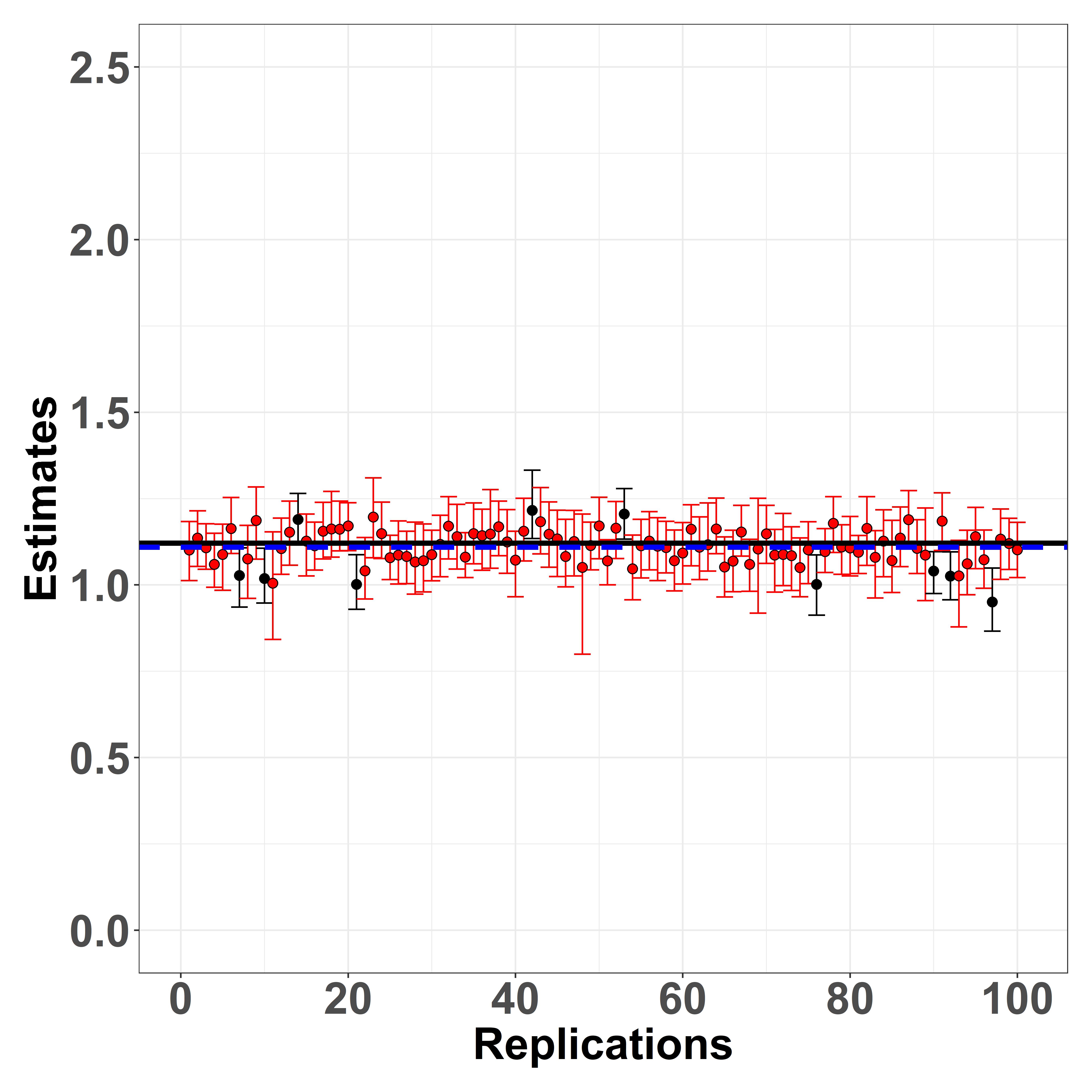
(a) SPSBP prior-Weibull kernel

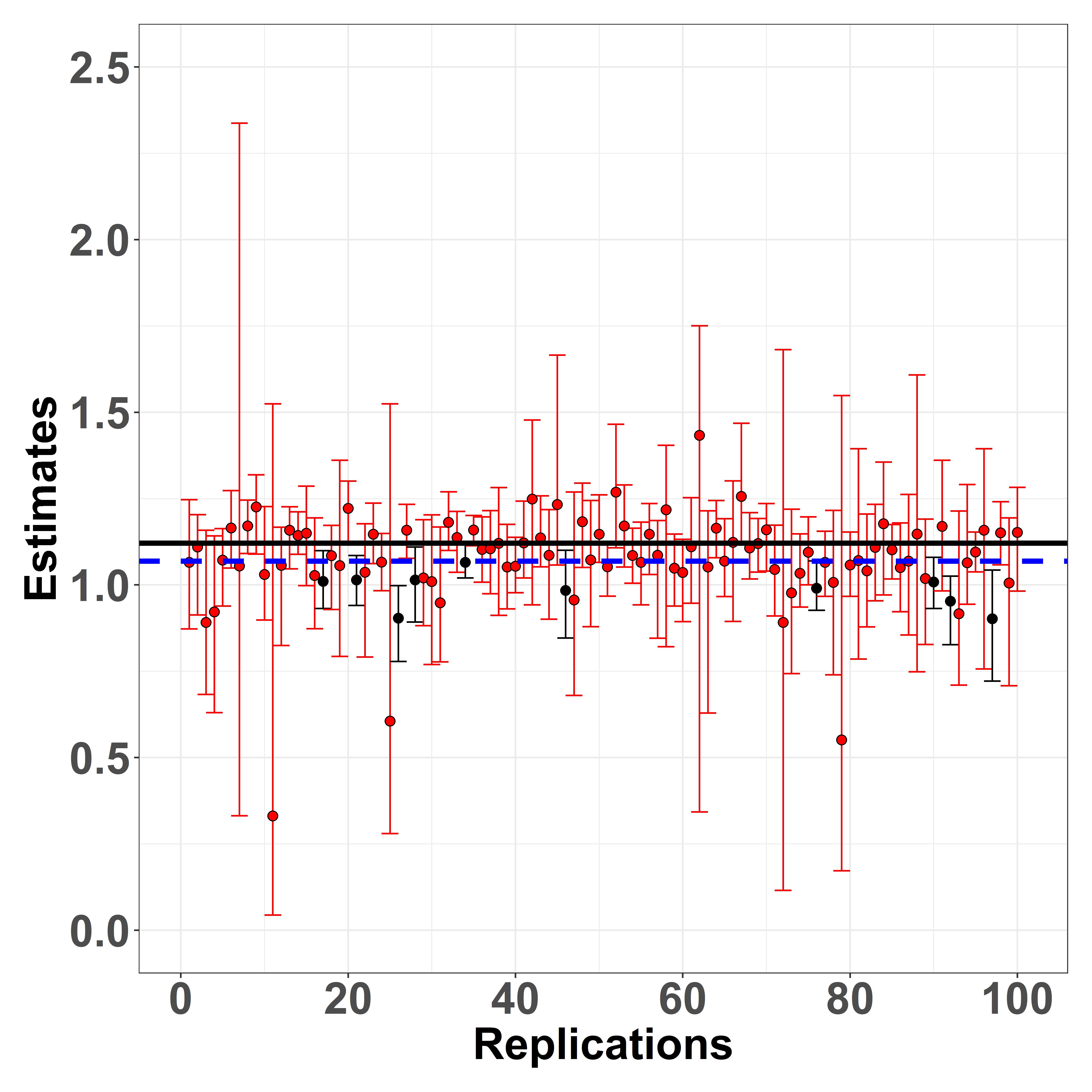
(b) PSBP prior-Weibull kernel

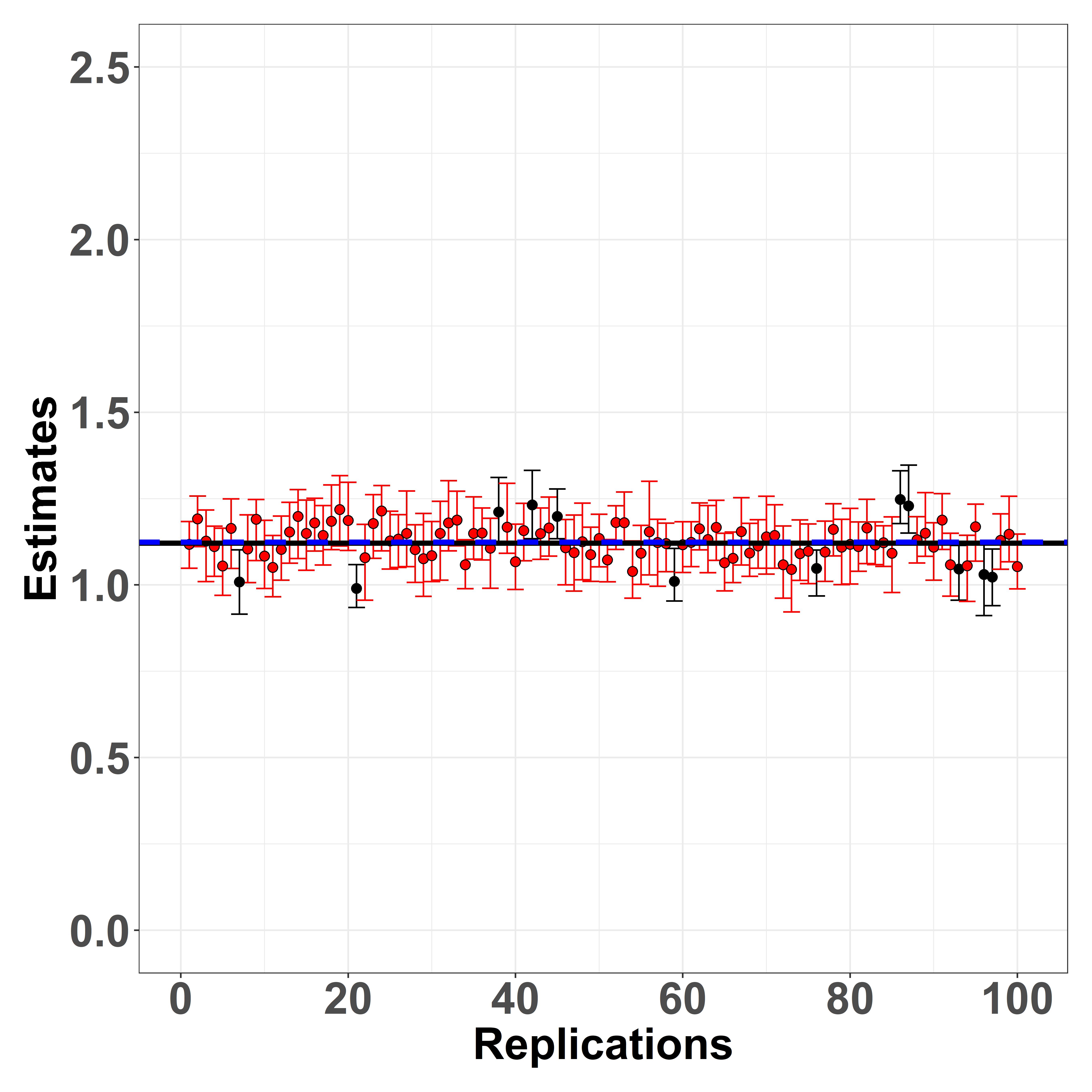
(c) LSBP prior-Weibull kernel

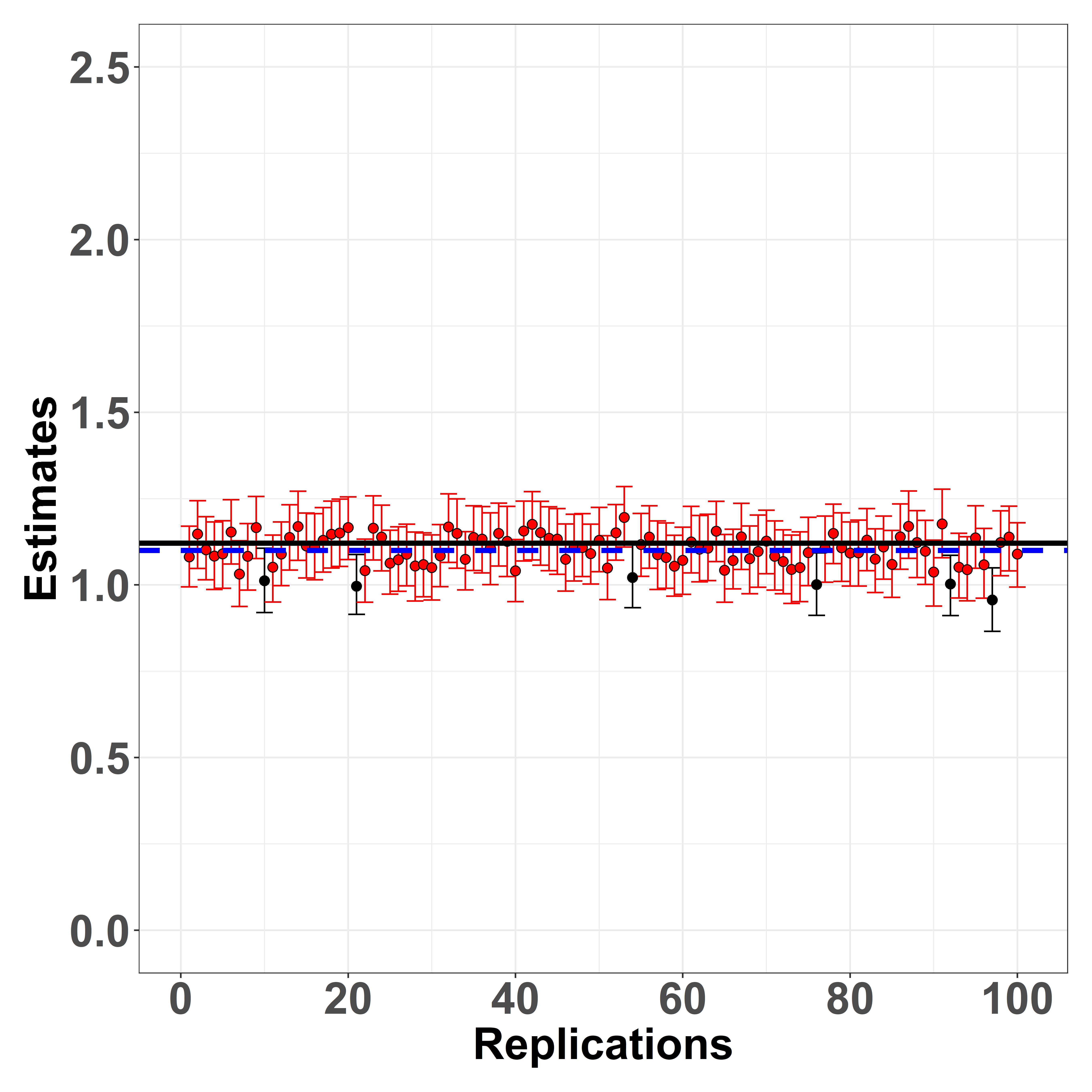
(d) LDDP prior-Weibull kernel

RMSTD evaluated at $\tau=5$ years; coefficients of predictor effects: $(\beta_{A}=2.5,\beta_{W_{1}}=1.5,\beta_{W_{2}}=2.5,\beta_{W_{3}}=1.3)$; black solid lines and blue dashed lines mark the true RMSTD value and average RMSTD point estimates, respectively.

Figure 6: Single time point analysis scenario S1: ATE point estimates with 95% credible intervals comparing 4 prior models (2-components Weibull data generation model under an RCT setting; $\tau=5$)

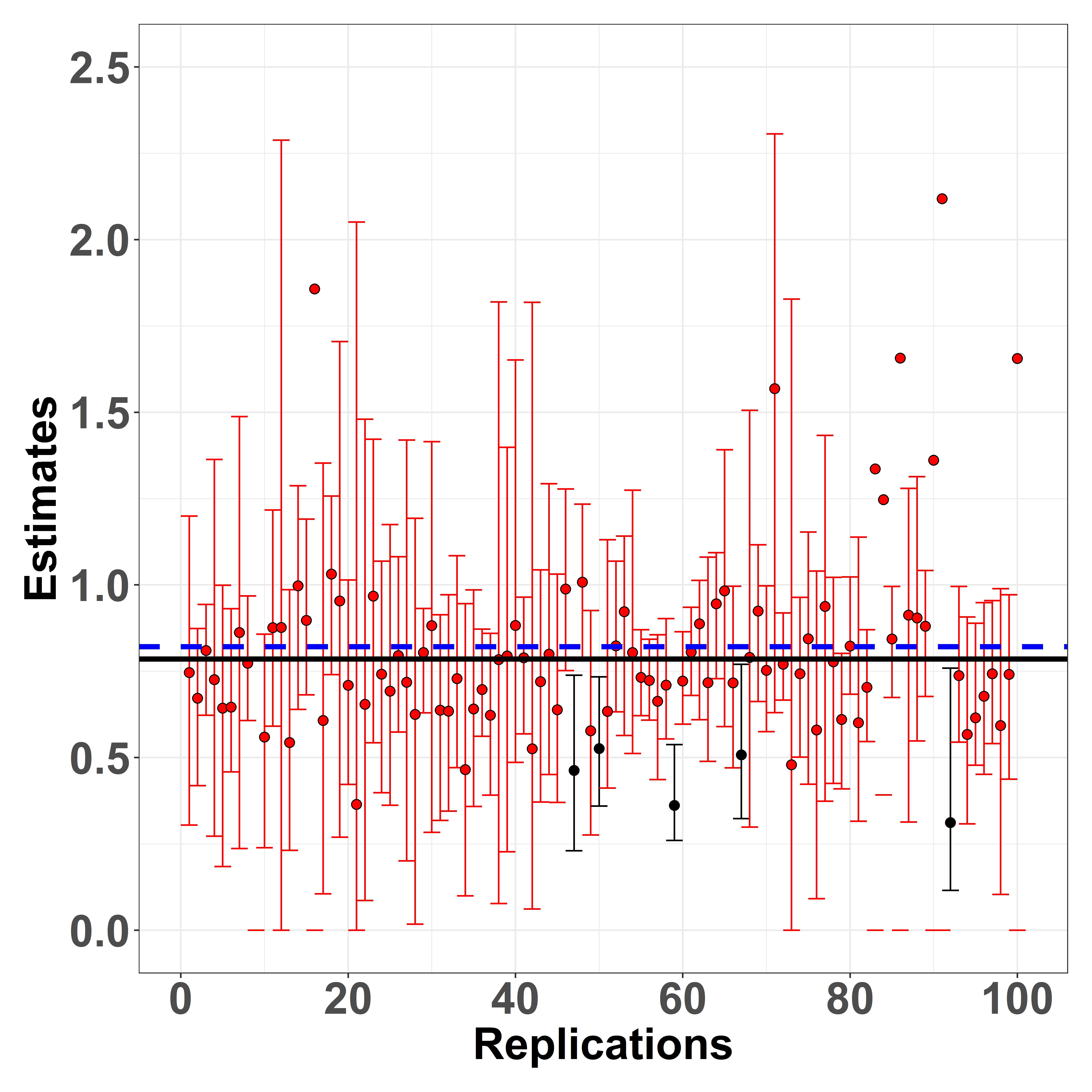
(a) SPSBP prior-Weibull kernel

(b) PSBP prior-Weibull kernel

(c) LSBP prior-Weibull kernel

(d) LDDP prior-Weibull kernel

RMSTD evaluated at $\tau=5$ years; coefficients of predictor effects: $(\beta_{A}=2.5,\beta_{W_{1}}=1.5,\beta_{W_{2}}=2.5,\beta_{W_{3}}=1.3)$; black solid lines and blue dashed lines mark the true RMSTD value and average RMSTD point estimates, respectively.

Figure 7: Subject level RMST predictions scenario 1-B: subject versus bias; data are generated under the two-components Weibull mixture model; $\tau=5$

Figure 8: Subject level RMST predictions scenario 1-C: $\bm{w}_{i}^{tr}\beta_{2Weibull}(i=\{1,\ldots,N\})$ versus bias; data are generated under the two-components Weibull mixture model; $\tau=5$

Real Data Analysis Results

Figure 9 shows survival probabilities estimated for the two treatment groups of PRIME trial data on the OS endpoint among KRAS WT patients. A Cox proportional hazards model (Therneau and Grambsch,, 2000) that adjusts for body mass index (BMI) and age was fitted. Both point estimates (colored solid lines) and $95\%$ confidence intervals (colored shades) are presented, and median survival time is marked by black dotted lines.

Figure 9: Estimated survival probabilities

A Cox proportional hazards model (Therneau and Grambsch,, 2000) that adjusts for bmi and kras is fitted to estimate survival probabilities; both point estimates (colored solid lines) and $95\%$ confidence intervals (colored shades) are presented; median survival time is marked by black dotted lines.

Table 3: REAL DATA RMSTD CURVE ANALYSIS

Method	$\tau$ (years)	0.5	1	1.5	2	2.5	3	3.5
LSBP Weibull	$95\%$ CI Lower	0.00	0.00	0.00	0.00	0.00	0.00	-0.01
	Point Estimate	0.01	0.02	0.04	0.08	0.11	0.14	0.15
	$95\%$ CI Upper	0.01	0.04	0.09	0.16	0.22	0.27	0.31
SPSBP Weibull	$95\%$ CI Lower	0.00	-0.01	-0.02	-0.03	-0.04	-0.06	-0.07
	Point Estimate	0.00	0.02	0.04	0.06	0.09	0.11	0.12
	$95\%$ CI Upper	0.01	0.04	0.10	0.16	0.22	0.26	0.30
PSBP Weibull	$95\%$ CI Lower	0.00	0.00	0.00	0.00	0.00	0.00	0.00
	Point Estimate	0.01	0.03	0.07	0.13	0.19	0.24	0.29
	$95\%$ CI Upper	0.02	0.07	0.15	0.26	0.38	0.49	0.59
LSBP Gamma	$95\%$ CI Lower	0.00	0.00	0.00	0.00	0.00	0.00	0.00
	Point Estimate	0.00	0.02	0.04	0.07	0.11	0.14	0.17
	$95\%$ CI Upper	0.01	0.04	0.09	0.15	0.22	0.28	0.34
SPSBP Gamma	$95\%$ CI Lower	0.00	-0.01	-0.01	-0.02	-0.02	-0.03	-0.03
	Point Estimate	0.00	0.02	0.04	0.07	0.10	0.13	0.15
	$95\%$ CI Upper	0.01	0.05	0.10	0.16	0.23	0.30	0.37
PSBP Gamma	$95\%$ CI Lower	-0.01	-0.03	-0.06	-0.10	-0.15	-0.20	-0.25
	Point Estimate	0.00	0.01	0.03	0.05	0.07	0.09	0.11
	$95\%$ CI Upper	0.01	0.05	0.10	0.17	0.24	0.31	0.38
Tian et al., (2014)	$95\%$ CI Lower	-0.01	-0.02	-0.03	-0.03	-0.02	-0.01	-0.04
	Point Estimate	0.01	0.01	0.03	0.07	0.11	0.14	0.14
	$95\%$ CI Upper	0.02	0.05	0.10	0.16	0.24	0.30	0.33

Additional Results

Linear Dependent Dirichlet Process Mixture Models

We can model a density function through a Dirichlet process mixture (DPM) model: $f(y)=\int K_{\bm{\theta}}(y)\;dG(\bm{\theta})$ where $G\sim DP(\alpha,G_{0})$.

Alternatively, we can incorporate covariates dependence on (certain) parameter(s) of the kernel density, which results in a LDDP mixture model:

$$f(y)=\int K\big{(}y\;|\;\bm{\theta}(\bm{w})\big{)}\;dG\big{(}\bm{\theta}(\bm{w})\big{)};\quad G\sim DP(\alpha,G_{0})$$ (22)

where $\bm{\theta}(\bm{w})=\big{(}\bm{\psi}(\bm{w})^{T}\bm{\beta},\bm{\omega}\big{)}$. The DP prior is assigned on $\bm{\beta}$ and $\bm{\omega}$: $(\bm{\beta},\bm{\omega})\sim G$ where $\bm{\beta}=\{\bm{\beta}_{1},\ldots,\bm{\beta}_{R}\}$ for adjusting $R$ predictors. In the above formulation, covariates dependence are only introduced on the point masses (atoms), which categorize it as a single-$\pi$ DDP model Quintana et al., (2022). For the $h^{th}$ cluster,

$$\begin{split}&y_{i}\ |\ \bm{\beta}_{i,h},\omega_{h}\stackrel{{\scriptstyle i.i.d.}}{{\sim}}K\big{(}y_{i}\;|\;exp\big{\{}\bm{\psi}(\bm{w}_{i})^{tr}\bm{\beta}_{i,h}\big{\}},\omega_{h}\big{)},\quad i=1,\ldots,N\\ &v_{h}\sim Beta(1,M),\;\pi_{1}=v_{1}\\ &\pi_{h}=\big{(}1-v_{1}\big{)}\big{(}1-v_{2}\big{)}\ldots\big{(}1-v_{h-1}\big{)}v_{h},\quad h\in\{2,\ldots,L-1\}\\ &\bm{\beta}_{h}=\{\beta_{h,A},\beta_{h,1},\ldots,\beta_{h,R}\}\sim\mathcal{N}_{R+1}(\bm{\mu}_{\beta},\bm{\Sigma}_{\beta}),\quad h\in\{1,\ldots,L\}\\ &\omega_{h}\sim unif(c_{low},c_{up}),\quad h\in\{1,\ldots,L\}\end{split}$$ (23)

where $(M,\bm{\mu}_{\beta},\bm{\Sigma}_{\beta},c_{low},c_{up})$ are constants. For more flexibility, one could model $M\sim Gamma(a_{\alpha},b_{\alpha})$ given constants $(a_{\alpha},b_{\alpha})$. As previously stated, we can choose $K(y_{i}\;|\;\cdot)$ to be either a Weibull kernel density (scale$=exp\big{\{}\bm{\psi}(\bm{w}_{i})^{tr}\bm{\beta}_{ih}\big{\}}$, shape$=\omega_{h}$) or a gamma kernel density (rate$=exp\big{\{}\bm{\psi}(\bm{w}_{i})^{tr}\bm{\beta}_{ih}\big{\}}$, shape$=\omega_{h}$) whose support is on $\mathbb{R}^{+}$.

Subsequently, its log joint density is

$$\begin{split}&\mathcal{Q}\big{(}\bm{\theta}=(\bm{\beta},\bm{\omega},M),\bm{o}\big{)}=\prod_{i=1}^{N}\Big{\{}\big{[}f_{\bm{\theta}}(y_{i})\big{(}1-H(y_{i})\big{)}\big{]}^{\delta_{i}}\big{[}S_{\bm{\theta}}(y_{i})h(y_{i})\big{]}^{(1-\delta_{i})}\Big{\}}\\ &\propto\prod_{i=1}^{N}\big{[}f_{\bm{\theta}}(y_{i})^{\delta_{i}}S_{\bm{\theta}}(y_{i})^{(1-\delta_{i})}\big{]}\\ &\propto\prod_{i=1}^{N}\sum_{j=1}^{L}\pi_{j}\cdot\Big{[}K\big{(}y_{i}\;|\;exp\big{\{}\bm{\psi}(\bm{w}_{i})^{tr}\bm{\beta}_{i,j}\big{\}},\omega_{j}\big{)}\Big{]}^{\delta_{i}}\cdot\Big{[}\int_{t}^{\infty}K\big{(}y_{i}\;|\;exp\big{\{}\bm{\psi}(\bm{w}_{i})^{tr}\bm{\beta}_{i,j}\big{\}},\omega_{j}\big{)}\Big{]}^{(1-\delta_{i})}\\ &\propto\prod_{i=1}^{N}\sum_{j=1}^{L}\Big{\{}v_{j}\prod_{l<j}\big{[}1-v_{l}\big{]}\Big{\}}\\ &\cdot\Big{[}K\big{(}y_{i}\;|\;exp\big{\{}\bm{\psi}(\bm{w}_{i})^{tr}\bm{\beta}_{i,j}\big{\}},\omega_{j}\big{)}\Big{]}^{\delta_{i}}\cdot\Big{[}\int_{t}^{\infty}K\big{(}y_{i}\;|\;exp\big{\{}\bm{\psi}(\bm{w}_{i})^{tr}\bm{\beta}_{i,j}\big{\}},\omega_{j}\big{)}\Big{]}^{(1-\delta_{i})}\end{split}$$ (24)

where $v_{j}\sim Beta(1,M)$, $\bm{\beta}=\{\bm{\beta}_{i,j}\;|\;i=1,\ldots,N,j=1,\ldots,L\};\;\bm{\beta}_{i,j}=\{\bm{\beta}_{i,j,1},\ldots,\bm{\beta}_{i,j,R}\}$, $\bm{\omega}=\{\omega_{1},\ldots,\omega_{L}\}$, $\bm{o}=\{\bm{o}_{1},\ldots,\bm{o}_{N}\};\;o_{i}=\{y_{i},\delta_{i},\bm{w}_{i}\}$.

Single-Atoms Dependent Stick-Breaking Process Prior Mixture Models

We can model the RMST function by assigning a single-atoms DSBP prior . This modeling approach assumes predictor dependence only on the mixing probabilities, which resembles a single-atoms dependent Dirichlet process prior mixture model. With a slight abuse of notations, let $\bm{\omega}=\{\omega_{1},\omega_{2}\}$ denote the parameters of a two-parameter kernel density. For this approach, we model both parameters $\{\omega_{1},\omega_{2}\}$ assuming a (generalized) stick-breaking process prior, without incorporating covariates-dependence on the kernel densities.

For the $h^{th}$ cluster,

$$\begin{split}&y_{i}\ |\ \omega_{1,h},\omega_{2,h}\stackrel{{\scriptstyle i.i.d.}}{{\sim}}K\big{(}y_{i}\;|\;\omega_{1,h},\omega_{2,h}\big{)},\quad i=1,\ldots,N\\ &v_{h}(\bm{w}_{i})=g(\bm{\psi}(\bm{w}_{i})^{tr}\alpha_{h}),\;\pi_{1}(\bm{w}_{i})=v_{1}(\bm{w}_{i})\\ &\pi_{h}(\bm{w}_{i})=\big{(}1-v_{1}(\bm{w}_{i})\big{)}\big{(}1-v_{2}(\bm{w}_{i})\big{)}\ldots\big{(}1-v_{h-1}(\bm{w}_{i})\big{)}v_{h}(\bm{w}_{i}),\quad h\in\{2,\ldots,L-1\}\\ &\bm{\alpha}_{h}=\{\alpha_{h,A},\alpha_{h,1},\ldots,\alpha_{h,R}\}\sim\mathcal{N}_{R+1}(\bm{\mu}_{\alpha},\bm{\Sigma}_{\alpha}),\quad h\in\{1,\ldots,L-1\}\\ &\omega_{1,h}\sim unif(c_{low},c_{up}),\;\omega_{2,h}\sim unif(d_{low},d_{up}),\quad h\in\{1,\ldots,L\}\end{split}$$ (25)

where $(\bm{\mu}_{\alpha},\bm{\Sigma}_{\alpha},c_{low},c_{up},d_{low},d_{up})$ are constants. For more flexibility, one could model $\omega_{1}\sim Gamma(a_{1},b_{1});\;\omega_{2}\sim Gamma(a_{2},b_{2})$ given constants $(a_{1},b_{1},a_{2},b_{2})$. The log joint density is

$$\begin{split}&\mathcal{Q}\big{(}\bm{\theta}=(\bm{\alpha},\bm{\omega}_{1},\bm{\omega}_{2}),\bm{o}\big{)}=\prod_{i=1}^{N}\Big{\{}\big{[}f_{\bm{\theta}}(y_{i})\big{(}1-H(y_{i})\big{)}\big{]}^{\delta_{i}}\big{[}S_{\bm{\theta}}(y_{i})h(y_{i})\big{]}^{(1-\delta_{i})}\Big{\}}\\ &\propto\prod_{i=1}^{N}\big{[}f_{\bm{\theta}}(y_{i})^{\delta_{i}}S_{\bm{\theta}}(y_{i})^{(1-\delta_{i})}\big{]}\\ &\propto\prod_{i=1}^{N}\sum_{j=1}^{L}\pi_{j}(\bm{w}_{i})\cdot\Big{[}K\big{(}y_{i}\;|\;\omega_{1,j},\omega_{2,j}\big{)}\Big{]}^{\delta_{i}}\cdot\Big{[}\int_{t}^{\infty}K\big{(}y_{i}\;|\;\omega_{1,j},\omega_{2,j}\big{)}\Big{]}^{(1-\delta_{i})}\\ &\propto\prod_{i=1}^{N}\sum_{j=1}^{L}\Big{\{}v_{j}(\bm{w}_{i})\prod_{l<j}\big{[}1-v_{l}(\bm{w}_{i})\big{]}\Big{\}}\cdot\Big{[}K\big{(}y_{i}\;|\;\omega_{1,j},\omega_{2,j}\big{)}\Big{]}^{\delta_{i}}\cdot\Big{[}\int_{t}^{\infty}K\big{(}y_{i}\;|\;\omega_{1,j},\omega_{2,j}\big{)}\Big{]}^{(1-\delta_{i})}\\ &\propto\prod_{i=1}^{N}\sum_{j=1}^{L}\Big{\{}g(\bm{\psi}(\bm{w}_{i})^{tr}\bm{\alpha}_{i,j})\prod_{l<j}\big{[}1-g(\bm{\psi}(\bm{w}_{i})^{tr}\bm{\alpha}_{i,j})\big{]}\Big{\}}\cdot\Big{[}K\big{(}y_{i}\;|\;\omega_{1,j},\omega_{2,j}\big{)}\Big{]}^{\delta_{i}}\\ &\cdot\Big{[}\int_{t}^{\infty}K\big{(}y_{i}\;|\;\omega_{1,j},\omega_{2,j}\big{)}\Big{]}^{(1-\delta_{i})}\end{split}$$ (26)

where $\bm{\alpha}=\{\bm{\alpha}_{i,j}\;|\;i=1,\ldots,N,j=1,\ldots,L-1\};\;\bm{\alpha}_{i,j}=\{\bm{\alpha}_{i,j,1},\ldots,\bm{\alpha}_{i,j,R}\}$, $\bm{\omega}=\{\bm{\omega}_{1},\bm{\omega}_{2}\};\;\bm{\omega}_{1}=\{\omega_{1,1},\ldots,\omega_{1,L}\};\;\bm{\omega}_{2}=\{\omega_{2,1},\ldots,\omega_{2,L}\}$, $\bm{o}=\{\bm{o}_{1},\ldots,\bm{o}_{N}\};\;o_{i}=\{y_{i},\delta_{i},\bm{w}_{i}\}$.

Assuming a Weibull kernel density (scale=$\bm{\psi}(\bm{W})^{\prime}\bm{\beta}$, shape=$\omega$), (14) has a closed form

$$\begin{split}&\widehat{RMST}(t=\tau\;|\;\bm{w}_{i})=E_{\bm{\theta}}\Bigg{[}\sum_{h=1}^{L}\Bigg{\{}\pi_{h}\big{(}\bm{\psi}(\bm{w}_{i})^{\prime}\bm{\alpha}_{h}\big{)}\cdot\Big{[}\tau\cdot S_{i,h}(\tau)+\bm{\psi}(\bm{w}_{i})^{\prime}\bm{\beta}_{h}\cdot\\ &\gamma\big{(}\frac{1}{\omega_{h}}+1,\bm{\psi}(\bm{w}_{i})^{\prime}\bm{\beta}_{h}^{(-\omega_{h})}\tau^{\omega_{h}}\big{)}\Big{]}\Bigg{\}}\Bigg{]}\end{split}$$

where $\gamma(s,x)=\int_{0}^{x}t^{s-1}e^{-t}dt$ is the lower incomplete gamma function and $S_{i,h}(\tau)=exp\big{\{}-(\tau/\bm{\psi}(\bm{w}_{i})^{\prime}\bm{\beta}_{h})^{\omega_{h}}\big{\}}$.

Assuming a Gamma kernel density (rate=$\bm{\psi}(\bm{W})^{\prime}\bm{\beta}$, shape=$\omega$), (14) has a closed form

$$\begin{split}&\widehat{RMST}(t=\tau\;|\;\bm{w}_{i})=E_{\bm{\theta}}\Bigg{[}\sum_{h=1}^{L}\Bigg{\{}\pi_{h}\big{(}\bm{\psi}(\bm{w}_{i})^{\prime}\bm{\alpha}_{h}\big{)}\cdot\Big{\{}\tau+\\ &\Gamma(\omega_{h})^{-1}\Big{[}\frac{\omega_{h}\cdot\gamma\big{(}\omega_{h},\bm{\psi}(\bm{w}_{i})^{\prime}\bm{\beta}_{h}\tau\big{)}-\big{(}\bm{\psi}(\bm{w}_{i})^{\prime}\bm{\beta}_{h}\tau\big{)}^{\omega_{h}}e^{-\big{(}\bm{\psi}(\bm{w}_{i})^{\prime}\bm{\beta}_{h}\tau\big{)}}}{\bm{\psi}(\bm{w}_{i})^{\prime}\bm{\beta}_{h}}-\tau\cdot\gamma\big{(}\omega_{h},\bm{\psi}(\bm{w}_{i})^{\prime}\bm{\beta}_{h}\cdot\tau\big{)}\Big{]}\Big{\}}\Bigg{\}}\Bigg{]}\end{split}$$

given the property that $\gamma(s+1,x)=s\gamma(s,x)-x^{s}e^{-x}$ where $\gamma(s,x)=\int_{0}^{x}t^{s-1}e^{-t}dt$ is the lower incomplete gamma function and $\Gamma(\cdot)$ denotes the gamma function.

Define the causal RMSTD estimand and a BNP estimator as follows:

$$\Delta(\tau) =\text{RMST}_{A_{1}}(t=\tau)-\text{RMST}_{A_{0}}(t=\tau)$$

$$=\int_{0}^{\tau}E_{\bm{X}}\Big{[}S_{\bm{\theta}}(t\;|\;A=1,\bm{X})\Big{]}-E_{\bm{X}}\Big{[}S_{\bm{\theta}}(t\;|\;A=0,\bm{X})\Big{]}\;dt$$

$$\begin{split}\widehat{\Delta}&=E_{\bm{X}}\left[E_{\bm{\theta}}\left[\int_{0}^{\tau}S_{\bm{\theta}}(t\;|\;A=1,\bm{X}_{i}=\bm{x}_{i})-S_{\bm{\theta}}(t\;|\;A=0,\bm{X}_{i}=\bm{x}_{i})\;dt\right]\right]\\ &=\frac{1}{N}\sum_{i=1}^{N}E_{\bm{\theta}}\left[\int_{0}^{\tau}S_{\bm{\theta}}(t\;|\;A=1,\bm{X}_{i}=\bm{x}_{i})-S_{\bm{\theta}}(t\;|\;A=0,\bm{X}_{i}=\bm{x}_{i})\;dt\right]\\ &=\frac{1}{N}\sum_{i=1}^{N}E_{\bm{\theta}}\Bigg{[}\sum_{h=1}^{L}\Big{[}\pi_{h}\big{(}\bm{\psi}_{A1,1}(\bm{w}_{i})^{\prime}\bm{\alpha}_{h}\big{)}\int_{0}^{\tau}\int_{t}^{\infty}K\big{(}s\;|\;\bm{\psi}_{A1,2}(\bm{w}_{i})^{\prime}\bm{\beta}_{h},\bm{\omega}_{h}\big{)}\;dsdt\\ &-\pi_{h}\big{(}\bm{\psi}_{A0,1}(\bm{w}_{i})^{\prime}\bm{\alpha}_{h}\big{)}\int_{0}^{\tau}\int_{t}^{\infty}K\big{(}s\;|\;\bm{\psi}_{A0,2}(\bm{w}_{i})^{\prime}\bm{\beta}_{h},\bm{\omega}_{h}\big{)}\;dsdt\Big{]}\Bigg{]}\end{split}$$ (27)

References

• Ambrogi et al., (2022) Ambrogi, F., Iacobelli, S., and Andersen, P. K. (2022). Analyzing differences between restricted mean survival time curves using pseudo-values. BMC Medical Research Methodology, 22(1):1–12.
• Bokemeyer et al., (2009) Bokemeyer, C., Bondarenko, I., Makhson, A., Hartmann, J. T., Aparicio, J., De Braud, F., Donea, S., Ludwig, H., Schuch, G., Stroh, C., et al. (2009). Fluorouracil leucovorin and oxaliplatin with and without cetuximab in the first-line treatment of metastatic colorectal cancer. American Society of Clinical Oncology.
• Chen and Tsiatis, (2001) Chen, P.-Y. and Tsiatis, A. A. (2001). Causal inference on the difference of the restricted mean lifetime between two groups. Biometrics, 57(4):1030–1038.
• Chung and Dunson, (2009) Chung, Y. and Dunson, D. B. (2009). Nonparametric bayes conditional distribution modeling with variable selection. Journal of the American Statistical Association, 104(488):1646–1660.
• Cox, (1993) Cox, D. D. (1993). An analysis of bayesian inference for nonparametric regression. The Annals of Statistics, 21(2):903–923.
• Cunningham et al., (2004) Cunningham, D., Humblet, Y., Siena, S., Khayat, D., Bleiberg, H., Santoro, A., Bets, D., Mueser, M., Harstrick, A., Verslype, C., et al. (2004). Cetuximab monotherapy and cetuximab plus irinotecan in irinotecan-refractory metastatic colorectal cancer. New England Journal of Medicine, 351(4):337–345.
• Diaconis and Freedman, (1997) Diaconis, P. and Freedman, D. (1997). On the bernstein-von mises theorem with infinite dimensional parameters. Unpublished Manuscript.
• Diana et al., (2020) Diana, A., Matechou, E., Griffin, J., and Johnston, A. (2020). A hierarchical dependent dirichlet process prior for modelling bird migration patterns in the uk. The Annals of Applied Statistics, 14(1):473–493.
• Douillard et al., (2010) Douillard, J.-Y., Siena, S., Cassidy, J., Tabernero, J., Burkes, R., Barugel, M., Humblet, Y., Bodoky, G., Cunningham, D., Jassem, J., et al. (2010). Randomized, phase iii trial of panitumumab with infusional fluorouracil, leucovorin, and oxaliplatin (folfox4) versus folfox4 alone as first-line treatment in patients with previously untreated metastatic colorectal cancer: the prime study. Journal of clinical oncology, 28(31):4697–4705.
• Douillard et al., (2014) Douillard, J.-Y., Siena, S., Cassidy, J., Tabernero, J., Burkes, R., Barugel, M., Humblet, Y., Bodoky, G., Cunningham, D., Jassem, J., et al. (2014). Final results from prime: randomized phase iii study of panitumumab with folfox4 for first-line treatment of metastatic colorectal cancer. Annals of Oncology, 25(7):1346–1355.
• Dunson and Park, (2008) Dunson, D. B. and Park, J.-H. (2008). Kernel stick-breaking processes. Biometrika, 95(2):307–323.
• Dunson et al., (2007) Dunson, D. B., Pillai, N., and Park, J.-H. (2007). Bayesian density regression. Journal of the Royal Statistical Society: Series B (Statistical Methodology), 69(2):163–183.
• Freidlin et al., (2021) Freidlin, B., Hu, C., and Korn, E. L. (2021). Are restricted mean survival time methods especially useful for noninferiority trials? Clinical Trials, 18(2):188–196.
• Freidlin and Korn, (2019) Freidlin, B. and Korn, E. L. (2019). Methods for accommodating nonproportional hazards in clinical trials: ready for the primary analysis? Journal of Clinical Oncology, 37(35):3455.
• Giusti et al., (2007) Giusti, R. M., Shastri, K. A., Cohen, M. H., Keegan, P., and Pazdur, R. (2007). Fda drug approval summary: Panitumumab (vectibix™). The Oncologist, 12(5):577–583.
• Heinemann et al., (2009) Heinemann, V., Stintzing, S., Kirchner, T., Boeck, S., and Jung, A. (2009). Clinical relevance of egfr-and kras-status in colorectal cancer patients treated with monoclonal antibodies directed against the egfr. Cancer Treatment Reviews, 35(3):262–271.
• Irwin, (1949) Irwin, J. (1949). The standard error of an estimate of expectation of life, with special reference to expectation of tumourless life in experiments with mice. Epidemiology & Infection, 47(2):188–189.
• Ishwaran and James, (2001) Ishwaran, H. and James, L. F. (2001). Gibbs sampling methods for stick-breaking priors. Journal of the American Statistical Association, 96(453):161–173.
• Klein and Moeschberger, (2003) Klein, J. P. and Moeschberger, M. L. (2003). Survival analysis: techniques for censored and truncated data, volume 1230. Springer.
• Lieu et al., (2014) Lieu, C. H., Renfro, L. A., De Gramont, A., Meyers, J. P., Maughan, T. S., Seymour, M. T., Saltz, L., Goldberg, R. M., Sargent, D. J., Eckhardt, S. G., and Others (2014). Association of age with survival in patients with metastatic colorectal cancer: analysis from the ARCAD Clinical Trials Program. Journal of Clinical Oncology, 32(27):2975.
• Meier, (1975) Meier, P. (1975). Estimation of a distribution function from incomplete observations. Journal of Applied Probability, 12(S1):67–87.
• Morgan and Winship, (2015) Morgan, S. L. and Winship, C. (2015). Counterfactuals and causal inference. Cambridge University Press.
• Papageorgiou et al., (2015) Papageorgiou, G., Richardson, S., and Best, N. (2015). Bayesian non-parametric models for spatially indexed data of mixed type. Journal of the Royal Statistical Society: Series B (Statistical Methodology), 77(5):973–999.
• Pati and Dunson, (2014) Pati, D. and Dunson, D. B. (2014). Bayesian nonparametric regression with varying residual density. Annals of the Institute of Statistical Mathematics, 66(1):1–31.
• Poynor and Kottas, (2019) Poynor, V. and Kottas, A. (2019). Nonparametric bayesian inference for mean residual life functions in survival analysis. Biostatistics, 20(2):240–255.
• Quintana et al., (2022) Quintana, F. A., Müller, P., Jara, A., and MacEachern, S. N. (2022). The dependent dirichlet process and related models. Statistical Science, 37(1):24–41.
• Reich et al., (2007) Reich, B. J., Fuentes, M., et al. (2007). A multivariate semiparametric bayesian spatial modeling framework for hurricane surface wind fields. The Annals of Applied Statistics, 1(1):249–264.
• Ren et al., (2011) Ren, L., Du, L., Carin, L., and Dunson, D. B. (2011). Logistic stick-breaking process. Journal of Machine Learning Research, 12(1).
• Rigon and Durante, (2021) Rigon, T. and Durante, D. (2021). Tractable bayesian density regression via logit stick-breaking priors. Journal of Statistical Planning and Inference, 211:131–142.
• Rodriguez and Dunson, (2011) Rodriguez, A. and Dunson, D. B. (2011). Nonparametric bayesian models through probit stick-breaking processes. Bayesian analysis (Online), 6(1).
• Royston and Parmar, (2011) Royston, P. and Parmar, M. K. (2011). The use of restricted mean survival time to estimate the treatment effect in randomized clinical trials when the proportional hazards assumption is in doubt. Statistics in Medicine, 30(19):2409–2421.
• Royston and Parmar, (2013) Royston, P. and Parmar, M. K. (2013). Restricted mean survival time: an alternative to the hazard ratio for the design and analysis of randomized trials with a time-to-event outcome. BMC medical research methodology, 13(1):1–15.
• Szabó et al., (2015) Szabó, B., Van Der Vaart, A. W., and van Zanten, J. (2015). Frequentist coverage of adaptive nonparametric bayesian credible sets. The Annals of Statistics, 43(4):1391–1428.
• Therneau and Grambsch, (2000) Therneau, T. M. and Grambsch, P. M. (2000). The cox model. In Modeling survival data: extending the Cox model, pages 39–77. Springer.
• Tian et al., (2018) Tian, L., Fu, H., Ruberg, S. J., Uno, H., and Wei, L.-J. (2018). Efficiency of two sample tests via the restricted mean survival time for analyzing event time observations. Biometrics, 74(2):694–702.
• Tian et al., (2020) Tian, L., Jin, H., Uno, H., Lu, Y., Huang, B., Anderson, K. M., and Wei, L. (2020). On the empirical choice of the time window for restricted mean survival time. Biometrics, 76(4):1157–1166.
• Tian et al., (2014) Tian, L., Zhao, L., and Wei, L. (2014). Predicting the restricted mean event time with the subject’s baseline covariates in survival analysis. Biostatistics, 15(2):222–233.
• Uno et al., (2014) Uno, H., Claggett, B., Tian, L., Inoue, E., Gallo, P., Miyata, T., Schrag, D., Takeuchi, M., Uyama, Y., Zhao, L., et al. (2014). Moving beyond the hazard ratio in quantifying the between-group difference in survival analysis. Journal of clinical Oncology, 32(22):2380.
• Uno et al., (2015) Uno, H., Wittes, J., Fu, H., Solomon, S. D., Claggett, B., Tian, L., Cai, T., Pfeffer, M. A., Evans, S. R., and Wei, L.-J. (2015). Alternatives to hazard ratios for comparing the efficacy or safety of therapies in noninferiority studies. Annals of internal medicine, 163(2):127–134.
• Wang and Schaubel, (2018) Wang, X. and Schaubel, D. E. (2018). Modeling restricted mean survival time under general censoring mechanisms. Lifetime data analysis, 24(1):176–199.
• Wei et al., (2015) Wei, Y., Royston, P., Tierney, J. F., and Parmar, M. K. (2015). Meta-analysis of time-to-event outcomes from randomized trials using restricted mean survival time: application to individual participant data. Statistics in Medicine, 34(21):2881–2898.
• Weir et al., (2021) Weir, I. R., Tian, L., and Trinquart, L. (2021). Multivariate meta-analysis model for the difference in restricted mean survival times. Biostatistics, 22(1):82–96.
• Zhang and Yin, (2022) Zhang, C. and Yin, G. (2022). Bayesian nonparametric analysis of restricted mean survival time. Biometrics, pages 1–14.
• Zhang and Schaubel, (2012) Zhang, M. and Schaubel, D. E. (2012). Double-robust semiparametric estimator for differences in restricted mean lifetimes in observational studies. Biometrics, 68(4):999–1009.