Supermodular Rank:
Set Function Decomposition and Optimization

Abstract

We define the supermodular rank of a function on a lattice. This is the smallest number of terms needed to decompose it into a sum of supermodular functions. The supermodular summands are defined with respect to different partial orders. We characterize the maximum possible value of the supermodular rank and describe the functions with fixed supermodular rank. We analogously define the submodular rank. We use submodular decompositions to optimize set functions. Given a bound on the submodular rank of a set function, we formulate an algorithm that splits an optimization problem into submodular subproblems. We show that this method improves the approximation ratio guarantees of several algorithms for monotone set function maximization and ratio of set functions minimization, at a computation overhead that depends on the submodular rank.
Keywords: supermodular cone, imset inequality, set function optimization, greedy algorithm, approximation ratio

1 Introduction

We study the optimization of set functions – functions that are defined over families of subsets. The optimization of set functions is encountered in image segmentation ([7]), clustering ([39]), feature selection ([47]), and data subset selection ([54]). Brute force optimization is often not viable since the individual function evaluations may be expensive and the search space has exponential size. Therefore, one commonly relies on optimization heuristics that work for functions with particular structure. A classic function structure is supermodularity, which for a function on a lattice requires that $f(x)+f(y)\leq f(x\wedge y)+f(x\vee y)$. Supermodularity can be regarded as a discrete analogue of convexity. A function is submodular if its negative is supermodular. Submodularity is interpreted as a “diminishing returns” property. Sub- and supermodularity can be used to obtain guarantees for greedy optimization of functions on a lattice, in a similar way as convexity and concavity are used in iterative local optimization of functions on a vector space. Well-known examples are the results of [40] for greedy maximization of a monotone submodular set function subject to cardinality constraints and those of [10] for arbitrary matroid constraints. Refinements have been obtained using gradations such as total curvature ([12, 52, 18]).

As many set functions of interest are not sub- or supermodular, relaxations have been considered, such as the submodularity ratio ([14]), generalized curvature ([12, 5, 9, 20]), weak submodularity ([11, 23]), $\epsilon$-submodularity ([27]), submodularity over subsets ([15]), or bounds by submodular functions ([25]). We will discuss some of these works in more detail in Section 4.

We propose a new approach to grade the space of functions on a lattice. We define the supermodular rank of a function to be the smallest number of terms in a decomposition into a sum of functions that are $\pi$-supermodular, where $\pi$ is a partial order on the domain. The partial order $\pi$ differs between summands. We define the submodular rank analogously. We consider multivariate functions with partial orders that are products of arbitrary linear orders. We focus on set functions that are real-valued on $2^{[n]}\cong\{0,1\}^{n}$, with partial order defined by an order on the values $\{0,1\}$ of each input coordinate. We refine submodular rank to elementary partial orders, restricted to vary from a reference order by a transpositions in one input coordinate. We optimize set functions via submodular decompositions. The key insight for our optimization algorithms is that a function with elementary submodular rank $r$ can be split into $2^{r}$ submodular pieces. The gradation of non-submodular pieces, via the elementary submodular rank, lets us obtain improved optimization guarantees.

The supermodular functions are defined by linear inequalities, hence they comprise a polyhedral cone, which is called the supermodular cone. These inequalities are called imset inequalities in the study of conditional independence structures and graphical models ([51]). They impose non-negative dependence of conditional probabilities. The supermodular cone has been a subject of intensive study ([33, 50]), especially the characterization of its extreme rays ([26, 49]), which in general remains an open problem. Supermodular inequalities appear in semi-algebraic description of probabilistic graphical models with latent variables, such as mixtures of product distributions ([2]). [45] suggested that restricted Boltzmann machines could be described using Minkowski sums of supermodular cones (see Appendix I). We obtain the inequalities defining Minkowski sums of supermodular cones, which could be of interest in the description of latent variable graphical models.

Main contributions.

• We introduce the notion of supermodular rank for functions on partially ordered sets (Definition 9). The functions of supermodular rank at most $r$ comprise a union of Minkowski sums of at most $r$ supermodular cones. We characterize the facets of these sums (Theorem 8) and find the maximum supermodular rank (Theorems 10) and maximum elementary supermodular rank (Theorem 14).

• We describe a procedure to compute low supermodular rank approximations of functions via existing methods for highly constrained convex optimization (Section 3).

• We show that the supermodular rank decomposition provides a grading of set functions that is useful for obtaining optimization guarantees. We propose the r-split and r-split ratio algorithms for monotone set function and ratio of set functions optimization (Algorithms 2 and 4), which can trade off between computational cost and accuracy, with theoretical guarantees (Theorems 25, 30 and 31). These improve on previous guarantees for greedy algorithms based on approximate submodularity (Tables 2 and 3).

• Experiments illustrate that our methods are applicable in diverse settings and can significantly improve the quality of the solutions obtained upon optimization (Section 5).

2 Supermodular Cones

In this section we introduce our settings and describe basic properties with proofs in Appendix B.

Definition 1.

Let $X$ be a set with a partial order such that for any $x,y\in X$, there is a greatest lower bound $x\wedge y$ and a least upper bound $x\vee y$ (this makes $X$ a lattice). A function $f\colon X\to\mathbb{R}$ is supermodular if, for all $x,y\in X$,

$$f(x)+f(y)\leq f(x\wedge y)+f(x\vee y).$$ (1)

The function $f$ is submodular (resp. modular) if $\leq$ in (1) is replaced by $\geq$ (resp. $=$).

Definition 2.

We fix $X=\{0,1\}^{n}$ and consider a tuple of linear orders $\pi=(\pi_{1},\ldots,\pi_{n})$ on $\{0,1\}$. Our partial order is the product of the linear orders: for any $x,y\in X$, we have $x\leq_{\pi}y$ if and only if $x_{i}\leq_{\pi_{i}}y_{i}$ for all $i\in[n]$. For each $i$, there are two possible choices of $\pi_{i}$, the identity $0\leq_{\pi_{i}}1$, and the transposition $1\leq_{\pi_{i}}0$. A function that is supermodular with respect to $\pi$ is called $\pi$-supermodular.

For fixed $X$, the condition of $\pi$-supermodularity is defined by requiring that certain homogeneous linear inequalities hold. Hence the set of $\pi$-supermodular functions on $X$ is a convex polyhedral cone. We denote this cone by $\mathcal{L}_{\pi}\subseteq\mathbb{R}^{X}$. Two product orders generate the same supermodular cone if and only if one is the total reversion of the other, and hence there are $\frac{1}{2}\prod_{i}|X_{i}|!$ distinct cones $\mathcal{L}_{\pi}$, see [2]. The cone of $\pi$-submodular functions on $X$ is $-\mathcal{L}_{\pi}$.

In the case $X=\{0,1\}^{n}$, the description of the supermodular cone in Equation 1 involves $\binom{2^{n}}{2}$ linear inequalities, one for each pair $x,y\in X$. However, the cone can be described using just $\binom{n}{2}2^{n-2}$ facet-defining inequalities ([28]). These are the elementary imset inequalities ([51]). They compare $f$ on elements of $X$ that take the same value on all but two coordinates. Identifying binary vectors of length $n$ with their support sets in $[n]$, the elementary imset inequalities are

$$f(z\cup\{i\})+f(z\cup\{j\})\leq f(z)+f(z\cup\{i,j\}),$$ (2)

where $i,j\in[n]$, $i\neq j$ and $z\subseteq[n]\setminus\{i,j\}$.

We partition the $\binom{n}{2}2^{n-2}$ elementary imset inequalities into $\binom{n}{2}$ sets of $2^{n-2}$ inequalities, as follows.

Definition 3.

For fixed $i,j\in[n]$, $i\neq j$, we collect the inequalities in Equation 2 for all $z\subseteq[n]\setminus\{i,j\}$ into matrix notation as $A^{(ij)}f\geq 0$. We call $A^{(ij)}\in\mathbb{R}^{2^{n-2}\times 2^{n}}$ the $(ij)$ elementary imset matrix. Each row of $A^{(ij)}$ has two entries equal to $1$ and two entries equal to $-1$.

The elementary imset characterization extends to $\pi$-supermodular cones $\mathcal{L}_{\pi}$ with general $\pi$.

Definition 4.

Fix a tuple $\pi=(\pi_{1},\ldots,\pi_{n})$ of linear orders on $\{0,1\}$. Its sign vector is $\tau=(\tau_{1},\ldots,\tau_{n})\in\{\pm 1\}^{n}$, where $\tau_{i}=1$ if $0<_{\pi_{i}}1$ and $\tau_{i}=-1$ if $1<_{\pi_{i}}0$.

Lemma 5.

Fix a tuple of linear orders $\pi$ with sign vector $\tau$. Then a function $f\colon\{0,1\}^{n}\to\mathbb{R}$ is $\pi$-supermodular if and only if $\tau_{i}\tau_{j}A^{(ij)}f\geq 0$, for all $i,j\in[n]$ with $i\neq j$.

Example 6 (Three-bit supermodular functions).

For $X=\{0,1\}^{3}$, we have $\frac{1}{2}2^{3}=4$ supermodular cones $\mathcal{L}_{\pi}$, given by sign vectors $\tau\in\{\pm 1\}^{3}$ up to global sign change. Each cone is described by $\binom{3}{2}\times 2^{1}=6$ elementary imset inequalities, collected into three matrices $A^{(ij)}\in\mathbb{R}^{2\times 8}$. By Lemma 5, the sign of the inequality depends on the product $\tau_{i}\tau_{j}$:

$\tau$	$A^{(12)}f$	$A^{(13)}f$	$A^{(23)}f$
$(1,1,1)$	$+$	$+$	$+$
$(-1,1,1)$	$-$	$-$	$+$
$(1,-1,1)$	$-$	$+$	$-$
$(1,1,-1)$	$+$	$-$	$-$

In Appendix H we show that supermodular cones have tiny relative volume, at most $(0.85)^{2^{n}}$.

3 Supermodular Rank

3.1 Minkowski Sums of Supermodular Cones

We describe the facet defining inequalities of Minkowski sums of $\pi$-supermodular cones. Given two cones $\mathcal{P}$ and $\mathcal{Q}$, their Minkowski sum $\mathcal{P}+\mathcal{Q}$ is the set of points $p+q$, where $p\in\mathcal{P}$ and $q\in\mathcal{Q}$. For a partial order $\pi$ with sign vector $\tau$, we sometimes write $\mathcal{L}_{\tau}$ for $\mathcal{L}_{\pi}$.

Example 7 (Sum of two three-bit supermodular cones).

We saw in Example 6 that there are $4$ distinct $\pi$-supermodular cones $\mathcal{L}_{\pi}$, each defined by $\binom{3}{2}2^{3-2}=6$ elementary imset inequalities. The inequalities defining the Minkowski sum $\mathcal{L}_{(1,1,1)}+\mathcal{L}_{(-1,1,1)}$ are $A^{(23)}f\geq 0$. That is, the facet inequalities of the Minkowski sum are those inequalities that hold on both individual cones.

We develop general results on Minkowski sums of cones and apply them to the case of supermodular cones in Appendix D. We show that the observation in Example 7 holds in general: sums of $\pi$-supermodular cones are defined by the facet inequalities that are common to all supermodular summands. In particular, the Minkowski sum is as large a set as one could expect.

Theorem 8 (Facet inequalities of sums of supermodular cones).

Fix a tuple of partial orders $\pi^{(1)},\ldots,\pi^{(m)}$. The Minkowski sum of supermodular cones $\mathcal{L}_{\pi^{(1)}}+\cdots+\mathcal{L}_{\pi^{(m)}}$ is a convex polyhedral cone whose facet inequalities are the facet defining inequalities common to all $m$ cones $\mathcal{L}_{\pi^{(i)}}$.

Proof idea.

Each $\mathcal{L}_{\pi^{(i)}}$ is defined by picking sides of a fixed set of hyperplanes. All supermodular cones are full dimensional. If two cones lie on the same side of a hyperplane, then so does their Minkowski sum. Hence the sum is contained in the cone defined by the facet defining inequalities common to all $m$ cones $\mathcal{L}_{\pi^{(i)}}$. We show that the sum fills this cone. This generalizes the fact that a full dimensional cone $\mathcal{P}\subseteq\mathbb{R}^{d}$ satisfies $\mathcal{P}+(-\mathcal{P})=\mathbb{R}^{d}$. ∎

3.2 Maximum Supermodular Rank

Definition 9.

The supermodular rank of a function $f\colon\{0,1\}^{n}\to\mathbb{R}$ is the smallest $r$ such that $f=f_{1}+\cdots+f_{r}$, where each $f_{i}$ is a $\pi$-supermodular function for some $\pi$.

Theorem 10 (Maximum supermodular rank).

For $n\geq 3$, the maximum supermodular rank of a function $f\colon\{0,1\}^{n}\to\mathbb{R}$ is $\lceil\log_{2}n\rceil+1$. Moreover, submodular functions in the interior of $-\mathcal{L}_{(1,\ldots,1)}$ have supermodular rank $\lceil\log_{2}n\rceil$.

Proof idea.

We find $\lceil\log_{2}n\rceil+1$ $\pi$-supermodular cones whose Minkowski sum fills the space. To remove as many inequalities as possible, we choose cones that share as few inequalities as possible, by Theorem 8. The sign vectors should differ at about $n/2$ coordinates, by Lemma 5. A recursive argument shows that $\lceil\log_{2}n\rceil+1$ cones suffices. ∎

Submodular functions $f$ in the interior of $-\mathcal{L}_{(1\ldots 1)}$ do not have full rank. They satisfy $A^{(ij)}f<0$. We believe that full rank functions $f$ do not satisfy $A^{(ij)}f>0$ or $A^{(ij)}f<0$, for any $i\neq j$.

Example 11.

A function $f\colon\{0,1\}^{3}\to\mathbb{R}$ can be written as a sum of at most three $\pi$-supermodular functions. Furthermore, there are functions that cannot be written as a sum of two $\pi$-supermodular functions. Indeed, Example 6 shows that any two $\pi$-supermodular cones share one block of inequalities, and three do not share any inequalities.

Definition 9 has implications for implicit descriptions of certain probabilistic graphical models: models with a single binary hidden variable as well as restricted Boltzmann machines (RBMs). Specifically, a probability distribution in the RBM model with $r$ hidden variables has supermodular rank at most $r$. We discuss these connections in Appendix I.

Table 1: Volumes

Submodular
$n$	rank 1	rank 2	rank 3	rank 4
3	12.5%	74.9%	100%	-
4	0.0072%	5.9%	100%	-
Elementary Submodular
$n$	rank 1	rank 2	rank 3	rank 4
3	3.14%	53.16%	100%	-
4	$6\cdot 10^{-4}$%	0.38%	29%	100%

3.3 Elementary Submodular Rank

We introduce a specialized notion of supermodular rank, which we call the elementary supermodular rank. This restricts to specific $\pi$. Later we focus on submodular functions, so we phrase the definition in terms of submodular functions.

Definition 12.

If $\pi$ has a unique coordinate $i$ with the sign of $\pi_{i}$ equal to $-1$, then we call $-\mathcal{L}_{\pi}$ an elementary submodular cone and we say that a function $f\in-\mathcal{L}_{\pi}$ is $\{i\}$-submodular.

Definition 13.

The elementary submodular rank of a function $f\colon\{0,1\}^{n}\to\mathbb{R}$ is the smallest $r+1$ such that $f=f_{0}+f_{i_{1}}+\cdots+f_{i_{r}}$, where $f_{0}\in-\mathcal{L}_{(1,\ldots,1)}$ and $f_{i_{j}}$ is $\{i_{j}\}$-submodular.

Theorem 14 (Maximum elementary submodular rank).

For $n\geq 3$, the maximum elementary submodular rank of a function $f\colon\{0,1\}^{n}\to\mathbb{R}$ is $n$. Moreover, a supermodular function in the interior of $\mathcal{L}_{(1,\ldots,1)}$ has elementary submodular rank $n$.

The proof is given in Appendix D.4 using similar techniques to Theorem 10. The relative volume of functions of different ranks is shown in Table 1, with details in Appendix H.

3.4 Low Elementary Submodular Rank Approximations

Given $f\colon\{0,1\}^{n}\to\mathbb{R}$ and a target rank $r$, we seek an elementary submodular rank-$r$ approximation of $f$. This is a function $g\colon\{0,1\}^{n}\to\mathbb{R}$ that minimizes $\|f-g\|_{\ell_{2}}$, with $g$ elementary submodular rank $r$. The set of elementary submodular rank $r$ functions is a union of convex cones, which is in general not convex. However, for fixed $\pi^{(1)},\ldots,\pi^{(r)}$, finding the closest point to $f$ in $\mathcal{L}_{\pi^{(1)}}+\cdots+\mathcal{L}_{\pi^{(r)}}$ is a convex problem. To find $g$, we compute the approximation for all rank $r$ convex cones and pick the function with the least error. Computing the projection onto each cone may be challenging, due to the number of facet-defining inequalities. We use a new method Project and Forget [48], detailed in Appendix E.

4 Set Function Optimization

The elementary submodular rank gives a gradation of functions. We apply it to set function optimization. The first application is to constrained set function maximization.

4.1 Maximization of Monotone Set Functions

Algorithm 1 Greedy

1:function Greedy($f$, $\mathcal{M}$)

2:  $S_{0}=\emptyset$, $F=\{e\in V:S_{0}\cup\{e\}\in\mathcal{M}\}$

3:  while $F\neq\emptyset$ do

4:    $e=\operatorname*{arg\,max}_{e\in F}\Delta(e|S_{k})$

5:    $S_{k+1}=S_{k}\cup\{e\}$

6:    $F=\{e\in V:S_{k+1}\cup\{e\}\in\mathcal{M}\}$

7:  end while

8:  return $S_{k}$

9:end function

We first present definitions and previous results.

Definition 15.

A set function $f\colon 2^{V}\to\mathbb{R}$ is

• monotone (increasing) if $f(A)\!\leq\!f(B)$ for all $A\!\subseteq\!B$,

• normalized if $f(\emptyset)=0$, and

• positive if $f(A)>0$ for all $A\in 2^{V}\setminus\{\emptyset\}$.

Examples of monotone submodular functions include entropy $S\mapsto H(X_{S})$ and mutual information $S\mapsto I(Y;X_{S})$. Unconstrained maximization gives an optimum at $S=V$, but when constrained to subsets with upper bounded cardinality the problem is NP-hard. The cardinality constraint is a type of matroid constraint.

Definition 16.

A system of sets $\mathcal{M}\subseteq 2^{V}$ is a matroid, if (i) $S\in\mathcal{M}$ and $T\subset S$ implies $T\in X$ and (ii) $S,T\in\mathcal{M}$ and $|T|+1=|S|$ implies $\exists e\in S\setminus T$ such that $T\cup\{e\}\in\mathcal{M}$. The matroid rank is the cardinality of the largest set in $\mathcal{M}$.

Problem 17.

Let $f$ be a monotone increasing normalized set function and let $\mathcal{M}\subseteq 2^{V}$ be a matroid. The $\mathcal{M}$-matroid constrained maximization problem is $\max_{S\in\mathcal{M}}f(S)$. The cardinality constraint problem is the special case $\mathcal{M}=\{S\subseteq V\colon|S|\leq m\}$, for a given $m\leq|V|$.

A natural approach to finding an approximate solution to cardinality constrained monotone set function optimization is by an iteration that mimics gradient ascent. Given $S\subseteq V$ and $e\in V$, the discrete derivative of $f$ at $S$ in direction $e$ is

$$\Delta(e|S)=f(S\cup\{e\})-f(S).$$

The Greedy algorithm ([40]) produces a sequence of sets starting with $S_{0}=\emptyset$, adding at each iteration an element $e$ that maximizes the discrete derivative subject to $S_{i}\cup\{e\}\in\mathcal{M}$ until no further additions are possible, see Algorithm 1.

Submodular functions.

A well-known result by [40] shows that Greedy has an approximation ratio (i.e., returned value divided by optimum value) of at least $(1-e^{-1})$ for monotone submodular maximization with cardinality constraints. [10, 18] show a polynomial time algorithm exists for the matroid constraint case with the same approximation ratio of $(1-e^{-1})$. These guarantees can be refined by measuring how far a submodular function is from being modular.

Definition 18 ([12]).

The total curvature of a normalized, monotone increasing submodular set function $f$ is

$$\hat{\alpha}:=\max_{e\in\Omega}\frac{\Delta(e|\emptyset)-\Delta(e|V\setminus\{e\})}{\Delta(e|\emptyset)},\quad\text{where $\Omega=\{e\in V\colon\Delta(e|\emptyset)>0\}$. }$$

It can be shown that $\hat{\alpha}=0$ if and only if $f$ is modular, and that $\hat{\alpha}\leq 1$ for any submodular $f$. Building on this, [52] presents a Non-Oblivious Local Search Greedy algorithm. They proved for any $\epsilon$ an approximation ratio of $(1-\hat{\alpha}e^{-1}+O(\epsilon))$ for the matroid constraint and that this approximation ratio is optimal. See Appendix F.

Approximately submodular functions.

To optimize functions that are not submodular, many prior works have looked at approximately submodular functions. We briefly discuss these here.

Definition 19.

Fix a non-negative monotone set function $f:2^{V}\to\mathbb{R}$.

• The submodularity ratio ([5, 53]) with respect to a set $X$ and integer $m$ is

  $$\gamma_{X,m}:=\min_{T\subset X,S\subset V,|S|\leq m,S\cap T=\emptyset}\frac{\sum_{e\in S}\Delta(e|T)}{\Delta(S|T)}.$$

  We drop the subscripts when $X=V$ and $m=|V|$.

• The generalized curvature ([5]) is the smallest $\alpha$ s.t. for all $T,S\in 2^{V}$ and $e\in S\setminus T$,

  $$\Delta(e|(S\setminus\{e\})\cup T)\geq(1-\alpha)\Delta(e|S\setminus\{e\}).$$

Remark 20.

For monotone increasing $f$, we have $\gamma\in[0,1]$, with $\gamma=1$ if and only if $f$ is submodular as well as $\alpha\in[0,1]$ and $\alpha=0$ iff $f$ is supermodular. Thus, if $\alpha=0$ and $\gamma=1$, then $f$ is modular. We compare these notions to the elementary submodular rank in Appendix F.5.

[5] obtained a guarantee of $\frac{1}{\alpha}(1-e^{-\alpha\gamma})$ for the Greedy algorithm on the cardinality constraint problem. For optimization of non-negative monotone increasing $f$ with general matroid constraints, [9, 11, 20] provide approximation guarantees that depend on $\gamma$ and $\alpha$.

Functions with bounded elementary rank.

Algorithm 2 r-Split

1:function r-Split($f$, $r$, $\mathcal{A}$ - subroutine)

2:  for $A\subseteq B\subseteq V$ with $|B|=r$ do

3:    run $\mathcal{A}$ on $f_{A,B}$

4:  end for

5:  run $\mathcal{A}$ on $f$ 

6:  return Best seen set

7:end function

We formulate an algorithm with guarantees for the optimization of set functions with bounded elementary submodular rank. We first give definitions and properties of low elementary submodular rank functions.

Definition 21.

Given $A\subseteq B\subseteq V$, define $\Pi(A,B):=\{C\subseteq V:C\cap B=A\}$. Given a set function $f:2^{V}\to\mathbb{R}$, we let $f_{A,B}$ denote its restriction to $\Pi(A,B)$.

Note that $\Pi(A,B)\cong 2^{V\setminus B}$. If $B=\{i\}$, then $f_{\{i\},B}$ and $f_{\emptyset,B}$ are the pieces of $f$ on the sets that contain (resp. do not contain) $i$. If $|B|=m$, then we have $2^{m}$ pieces, the choices of $A\subseteq B$.

Proposition 22.

A set function $f$ has elementary submodular rank $r+1$, with decomposition $f=f_{0}+f_{i_{1}}+\cdots+f_{i_{r}}$, if and only if $f_{A,B}$ is submodular for $B=\{i_{1},\ldots,i_{r}\}$ and any $A\subseteq B$.

The pieces $f_{A,B}$ behave well in terms of their submodularity ratio and curvature.

Proposition 23.

If $f$ is a set function with submodularity ratio $\gamma$ and generalized curvature $\alpha$, then $f_{A,B}$ has submodularity ratio $\gamma_{A,B}\geq\gamma$ and generalized curvature $\alpha_{A,B}\leq\alpha$.

We propose the algorithm r-Split, see Algorithm 2. The idea is to run Greedy, or another optimization method, on the pieces $f_{A,B}$ separately and then choose the best subset.

Definition 24.

We define

$$\alpha_{r}:=\min_{B\subseteq V,|B|\leq r}\left(\max_{A\subseteq B}\alpha_{A,B}\right)\quad\text{and}\quad\gamma_{r}:=\max_{B\subseteq V,|B|\leq r}\left(\min_{A\subseteq B}\gamma_{A,B}\right).$$

Theorem 25 (Guarantees for r-Split).

Let $\mathcal{A}$ be an algorithm for matroid constrained maximization of set functions, such that for any monotone, non-negative function $g\colon 2^{W}\to\mathbb{R}$, $|W|=m$, with generalized curvature $\alpha$ and submodularity ratio $\gamma$, algorithm $\mathcal{A}$ makes $O(q(m))$ queries to the value of $g$, where $q$ is a polynomial, and returns a solution with approximation ratio $R(\alpha,\gamma)$. If $f\colon 2^{[n]}\to\mathbb{R}$ is a monotone, non-negative function with generalized curvature $\alpha$, submodularity ratio $\gamma$, and elementary submodular rank $r+1$, then r-Split with subroutine $\mathcal{A}$ runs in time $O(2^{r}n^{r}q(n))$ and returns a solution with approximation ratio $\max\{R(\alpha,\gamma),R(\alpha_{r},1)\}$.

Proof idea.

A function of elementary rank $r+1$ can be split into $2^{r}$ submodular pieces, by Proposition 22. The r-Split algorithm looks at all possible ways of splitting. Since one of the splittings has all pieces submodular, we get the stated approximation guarantee. Details are in Appendix F. ∎

Remark 26 (Approximation ratio).

The approximation ratio $R(\alpha,\gamma)$ usually improves as $\gamma$ increases, as for the function $\frac{1}{\alpha}(1-e^{-\alpha\gamma})$ from [5]. The case $\gamma=1$ corresponds to the function being submodular. If we split an elementary rank-$(r+1)$ function into the appropriate $2^{r}$ pieces, then we run the subroutine $\mathcal{A}$ on submodular functions and hence obtain best available guarantees.

Remark 27 (Time complexity).

For fixed $r$ we give a polynomial time approximation algorithm for elementary submodular rank-$(r+1)$ functions. If we assume knowledge of the cones involved in a decomposition of $f$, then we need only optimize over one split, and we can drop the time complexity factor $n^{r}$. With the extra information about the decomposition, this is a fixed parameter tractable (FPT) time $O(1)$ approximation for monotone function maximization, parameterized by the elementary submodular rank. This suggests that determining the cones in the decomposition may be a difficult problem.

In Table 2 we instantiate several corollaries of Theorem 25 for specific choices of the subroutine and compare them with the prior work mentioned above (see Appendix F for details).

Table 2: Approximation ratios and time complexity for maximizing a monotone, normalized function $f$ on $2^{[n]}$ of total curvature $\hat{\alpha}$, generalized curvature $\alpha$, submodularity ratio $\gamma$, and elementary submodular rank $r+1$. Here $m$ is the bound in the cardinality constraint, and $\rho$ is the matroid rank in the Matroid constraint. Results with ^∗ are in expectation over randomization in the algorithm.

	Sub -modular	Low Rank	Card. Constr.	Matroid Constr.	Approximation Ratio	Time	Ref.
​​​​​​Prior Work		-	-		$1-e^{-1}$ ∗	$\tilde{O}(n^{8})$	[10]
		-		-	$1-\hat{\alpha}e^{-1}-O(\epsilon)$	$O(\epsilon^{-1}poly(n))$	[52]
	-	-		-	$\frac{1}{\alpha}(1-e^{-\alpha\gamma})$	$O(nm)$	[5]
	-	-	-		$(1+\gamma^{-1})^{-2}$	$O(n^{2})$	[11]
	-	-	-		$\frac{0.4\gamma^{2}}{\sqrt{\rho\gamma}+1}$	$O(n^{2})$	[20]
	-	-	-		$(1+(1-\alpha)^{-1})^{-1}$	$O(n^{2})$	[20]
This Work​​	-			-	$1-\hat{\alpha}e^{-1}-O(\epsilon)$	$O(\epsilon^{-1}2^{r}n^{r}\cdot poly(n))$	Cor 64
	-			-	$\frac{1}{\alpha_{r}}(1-e^{-\alpha_{r}})$	$O(2^{r}n^{r}\cdot nm)$	Cor 65
	-		-		$1-e^{-1}$ ∗	$\tilde{O}(2^{r}n^{r}\cdot n^{8})$	Cor 66

4.2 Minimization of Ratios of Set Functions

Algorithm 3 Ratio Greedy

1:function Ratio Greedy($f$,$g$)

2:  Initialize: $S_{0}=\emptyset$, $R=V$

3:  while $R\neq\emptyset$ do

4:    $u=\operatorname*{arg\,min}_{v\in R}\frac{f(\{v\}\cup S_{i})}{g(\{v\}\cup S_{i})}$

5:    $S_{i+1}=S_{i}\cup\{u\}$

6:    $R=\{v\in R:g(\{v\}\cup S_{i+1})>0\}$

7:  end while

8:  return $S_{i}$

9:end function

The second application of our decomposition is to minimize ratios of set functions. We give definitions and previous results, with details in Appendix F.

Problem 28.

Given set functions $f$ and $g$, we seek

$$\min_{S}\frac{f(S)}{g(S)}.$$

[4] obtain guarantees for Ratio Greedy, see Algorithm 3, for different submodular or modular combinations of $f$ and $g$. To quantify the approximation ratio for non-sub-/modular $f,g$, we need a few definitions.

Definition 29 ([6]).

• The generalized inverse curvature of a non-negative set function $f$ is the smallest $\tilde{\alpha}^{f}$ such that for all $T,S\in 2^{V}$ and for all $e\in S\setminus T$,

  $$\Delta(e|S\setminus\{e\})\geq(1-\tilde{\alpha}^{f})\Delta(e|(S\setminus\{e\})\cup T).$$

• The curvature of $f$ with respect to $X$ is $\hat{c}^{f}(X):=1-\frac{\sum_{e\in X}(f(X)-f(X\setminus\{e\})}{\sum_{e\in X}f(\{e\})}$.

It is known that $f$ is submodular if and only if $\tilde{\alpha}^{f}=0$. Using these notions, [42] obtain an approximation guarantee for minimization of $f/g$ with monotone submodular $f$ and monotone $g$, and [53] obtain a guarantee when both $f$ and $g$ are monotone.

Functions with bounded elementary rank.

Algorithm 4 r-Split Ratio

1:function r-Split Ratio($f,g$, $r$, $\mathcal{A}$ - Greedy Ratio)

2:  for $A\subseteq B\subseteq V$ with $|B|=r$ do

3:    run $\mathcal{A}$ on $f_{A,B}$ and $g_{A,B}$

4:  end for

5:  run $\mathcal{A}$ on $f,g$ 

6:  return Best seen set

7:end function

We formulate results for r-Split with Greedy Ratio subroutine, shown in Algorithm 4. We improve on previous guarantees if the functions have low elementary submodular rank. First, we split only $f$.

Theorem 30 (Guarantees for r-Split Greedy Ratio I).

For the minimization of $f/g$ where $f,g$ are normalized positive monotone functions, assume $f$ has elementary submodular rank $r+1$. Let $X^{*}$ be the optimal solution. Then r-Split with Greedy Ratio subroutine at a time complexity of $O(2^{r}n^{r}\cdot n^{2})$, has approximation ratio

$$\frac{1}{\gamma_{\emptyset,|X^{*}|}^{g}}\frac{|X^{*}|}{1+(|X^{*}|-1)(1-\hat{c}^{f}(X^{*}))}.$$

If, in addition, $g$ is submodular then the approximation ratio is $1/(1-e^{\hat{\alpha}^{f}-1})$.

The first statement provides the same guarantee as a result of [42] but for a more general class of functions. Our result can be interpreted as grading the conditions of [53] to obtain similar guarantees as the more restrictive results of [42]. Next, we split both $f$ and $g$.

Theorem 31 (Guarantees for r-Split Greedy Ratio II).

Assume $f$ and $g$ are normalized positive monotone functions, with elementary submodular ranks $r_{f}+1$ and $r_{g}+1$. For the minimization of $f/g$, the algorithm r-Split with Greedy Ratio subroutine at a time complexity of $O(2^{r_{f}+r_{g}}n^{r_{f}+r_{g}}\cdot n^{2})$, has approximation ratio

$$\frac{1}{1-e^{\hat{\alpha}^{f}-1}},$$

This improves the approximation ratio guarantee of [53] to that of [4], which was valid only if $f,g$ are both submodular. Table 3 compares our results with prior work.

Table 3: Approximation ratios and time complexity for minimizing $f/g$ for monotone, normalized functions $f$ and $g$ on $2^{[n]}$. Here $f$ has total curvature $\hat{\alpha}^{f}$, generalized curvature $\alpha^{f}$, generalized inverse curvature $\tilde{\alpha}^{f}$, curvature $\hat{c}^{f}$, and elementary submodular rank $r_{f}+1$. $g$ has submodularity ratio $\gamma^{g}$ and elementary submodular rank $r_{g}+1$. $X^{*}$ is the optimal solution. Prior works are discussed in detail in Appendix F.

	Numerator	Denominator	Approx. Ratio	Time	Ref.
Prior Work	Modular	Modular	1	$O(n^{2})$	[4]
	Modular	Submodular	$1-e^{-1}$	$O(n^{2})$	[4]
	Submodular	Submodular	$\frac{1}{1-e^{\hat{\alpha}^{f}-1}}$	$O(n^{2})$	[4]
	Submodular	-	$\frac{1}{\gamma_{\emptyset,|X^{*}|}^{g}}\frac{|X^{*}|}{1+(|X^{*}|-1)(1-\hat{c}^{f}(X^{*}))}$	$O(n^{2})$	[42]
	-	-	$\frac{1}{\gamma^{g}_{\emptyset,|X^{*}|}}\frac{|X^{*}|}{1+(|X^{*}|-1)(1-\alpha^{f})(1-\tilde{\alpha}^{f})}$	$O(n^{2})$	[53]
This Work	Low Rank	-	$\frac{1}{\gamma_{\emptyset,|X^{*}|}^{g}}\frac{|X^{*}|}{1+(|X^{*}|-1)(1-\hat{c}^{f}(X^{*}))}$	$O(2^{r_{f}}n^{r_{f}}\cdot n^{2})$	Thm 30
	Low Rank	Submodular	$\frac{1}{1-e^{\hat{\alpha}^{f}-1}}$	$O(2^{r_{f}}n^{r_{f}}\cdot n^{2})$	Thm 30
	Low Rank	Low Rank	$\frac{1}{1-e^{\hat{\alpha}^{f}-1}}$	​​​​$O(2^{r_{f}+r_{g}}n^{r_{f}+r_{g}}\cdot n^{2})$	Thm 31

5 Experiments

We present experiments to support our theoretical analysis. We consider four types of functions: Determinantal, Bayesian, Column, and Random, detailed in Appendix G.

Submodularity ratio and generalized curvature.

We compute $\alpha_{r}$ and $\gamma_{r}$ and the resulting approximation ratio guarantee for constrained maximization for functions of the four different types, for $n=8$ and log number of pieces $0\leq r\leq 4$. We report the mean and standard error for $50$ functions in each case. Figure LABEL:fig:boundk shows that the approximation ratio guarantee can increase quickly: for Determinantal it improves by 400% by $r=4$.

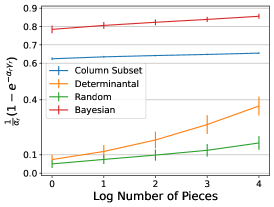
(a)

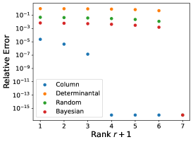
(b)

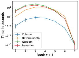
(c)

Figure 1: Shown are (a) how the bound from [5] changes when we use $\alpha_{r}$ and $\gamma_{r}$ (see Definition 24); higher values correspond to better guarantees, (b) the relative error when approximating a function by an elementary rank-$(r+1)$ function, and (c) the running times for computing the approximation.

Low elementary rank approximations.

We compute low elementary submodular rank approximations for $n=7$ and $1\leq r+1\leq 7$. Figure LABEL:fig:error shows the relative error ${\|f-g\|_{\ell_{2}}}/{\|f\|_{\ell_{2}}}$ and Figure LABEL:fig:times the running times (see Appendix E). We see that Column has a low elementary submodular rank, $r+1=4$. The computation time peaks near $r+1=n/2$ and decreases for larger $r+1$ as there are fewer Minkowski sums and fewer constraints.

r-Split Greedy with small $\bm{n}$.

We evaluate the improvement that r-Split provides over Greedy. Let $n=20$ and maximize functions with a cardinality constraint $m=10$. Figure LABEL:fig:ratio shows the approximation ratio for Greedy and r-Split Greedy for $r=1,2,3$, as well as how often the optimal solution was found. All four algorithms outperform their theoretical bounds. In all cases, increments in $r$ increase the percentage of times the (exact) optimal solution is found.

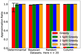
(a)

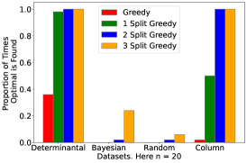
(b)

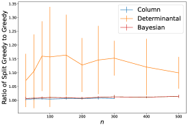
(c)

Figure 2: Shown are (a) the approximation ratio for the solution found versus the optimal solution averaged over 50 objective functions in each type, (b) the proportion of instances for which the algorithms find the optimal solution, (c) the ratio of the solution found by 1 Split and Greedy.

r-Split Greedy with large $\bm{n}$.

We now consider larger values of $n$, with a maximum cardinality of 15. Since we do not know the optimal solution, in Figure LABEL:fig:ratios we plot the ratio of r-Split Greedy to Greedy. For Bayesian our approach improves the quality of the solution found by about 1% and for Determinantal by 5–15% on average. Running the experiment for Random is not viable as we cannot store it for oracle access. Computing the Column function takes longer than computing Determinantal and Bayesian. Hence we only ran it until $n=300$. For $n=300$, there are $\binom{300}{15}\approx 8\times 10^{24}$ possible solutions.

6 Conclusion

We introduced the notion of sub-/supermodular rank for functions on a lattice along with geometric characterizations. Based on this we developed algorithms for constrained set function maximization and ratios of set functions minimization with theoretical guarantees improving several previous guarantees for these problems. Our algorithms do not require knowledge of the rank decomposition and show improved empirical performance on several commonly considered tasks even for small choices of $r$. For large $n$ it becomes unfeasible to evaluate all splits for large $r$, and one could consider evaluating only a random selection. It will be interesting to study in more detail the rank of typical functions. The theoretical complexity and practical approaches for computing rank decompositions remain open problems with interesting consequences. Another natural extension of our work is to consider general lattices, involving non-binary variables.

Acknowledgments

RS and GM have been supported in part by DFG SPP 2298 grant 464109215. GM has been supported by NSF CAREER 2145630, NSF 2212520, ERC Starting Grant 757983, and BMBF in DAAD project 57616814. AS was supported by the Society of Fellows at Harvard University.

Appendix A Notation

We summarize our notation in the following table.

[.5]() $[n]$	$\{1,\ldots,n\}$.
[.5]() $(X,\pi)$	A poset $X$ with partial order defined by a tuple $\pi$.
[.5]() $f$	A function from a poset $(X,\pi)$ to $\mathbb{R}$.
[.5]() $\mathcal{L_{\pi}}$	The cone of $\pi$-supermodular functions.
[.5]() $\pi$	Tuple of $n$ linear orders $\pi=(\pi_{1},\ldots,\pi_{n})$, see Definition 2.
[.5]() $A^{(ij)}$	The $(ij)$ elementary imset matrix, a $2^{n-2}\times 2^{n}$ matrix that collects the imset inequalities for each $x\in\{0,1\}^{n-2}$, see Definition 3.
[.5]() $\tau$	Sign vector $\tau=(\tau_{1},\ldots,\tau_{n})$ of a tuple of linear orders $\pi$, see Definition 4.
[.5]() $\xi$	Vector in $\{-1,0,1\}^{\binom{n}{2}}$, described in Definition 40.

Notions of curvature and submodularity ratio.

[.5]() $\hat{\alpha}$	The total curvature of a normalized, monotone increasing submodular function $f$ is $\hat{\alpha}:=\max_{e\in\Omega}\frac{\Delta(e|\emptyset)-\Delta(e|V\setminus\{e\})}{\Delta(e|\emptyset)}$, where $\Omega=\{e\in V\colon\Delta(e|\emptyset)>0\}$
[.5]() $\gamma_{X,m}$	The submodularity ratio of a non-negative monotone function w.r.t. set $X$ and integer $m$ is $\gamma_{X,m}:=\min_{T\subset X,S\subset V,|S|\leq m,S\cap T=\emptyset}\frac{\sum_{e\in S}\Delta(e|T)}{\Delta(S|T)}$. Subscripts dropped for $X=V$, $m=k$
[.5]() $\alpha$	The generalized curvature of a non-negative monotone set function is the smallest $\alpha$ s.t. for all $T,S\in 2^{V}$ and $e\in S\setminus T$, $\displaystyle\Delta(e|(S\setminus\{e\})\cup T)\geq(1-\alpha)\Delta(e|S\setminus\{e\})$
[.5]() $\tilde{\alpha}$	The generalized inverse curvature of a non-negative set function $f$ is the smallest $\tilde{\alpha}^{f}$ such that for all $T,S\in 2^{V}$ and for all $e\in S\setminus T$, $\displaystyle\Delta(e|S\setminus\{e\})\geq(1-\tilde{\alpha}^{f})\Delta(e|(S\setminus\{e\})\cup T).$
[.5]() $\hat{c}$	The curvature of $f$ with respect to $X$ is $\hat{c}^{f}(X):=1-\frac{\sum_{e\in X}(f(X)-f(X\setminus\{e\})}{\sum_{e\in X}f(\{e\})}$

Appendix B Background on Posets

We introduce relevant background for posets and partial orders.

Definition 32.

Let $(X,\preceq)$ be a partially ordered set (poset). Given two elements $x,y\in X$,

1. The greatest lower bound $x\wedge y$ is a $z\in X$ such that $z\prec x,y$ and $w\preceq z$ for all $w\prec x,y$.

2. The least upper bound $x\vee y$ is a $z\in X$ such that $x,y\prec z$ and $z\preceq w$ for all $x,y\prec w$.

Posets such that any two elements have a least upper bound and a greatest lower bound are called lattices.

Example 33.

1. Let $X$ be the power set of some set, with $\prec$ the inclusion order. Given $x,y\in X$, we have $x\wedge y=x\cap y$ and $x\vee y=x\cup y$.

2. Let $X=[d_{1}]^{\prime}\times[d_{2}]^{\prime}\times\cdots\times[d_{n}]^{\prime}$, where $[n]^{\prime}:=\{0,1,2,3,\ldots,n-1\}$. Fix $x=(x_{1},\ldots x_{n})$ and $y=(y_{1},\ldots,y_{n})$ in $X$. Let $x\prec y$ if and only if $x\neq y$ and $x_{i}\leq y_{i}$, for all $i=1,\ldots,n$, where $\leq$ is the usual ordering on natural numbers. Then $x\wedge y=(\min(x_{1},y_{1}),\ldots,\min(x_{n},y_{n}))$ and $x\vee y=(\max(x_{1},y_{1}),\ldots,\max(x_{n},y_{n}))$.

3. Let $X=X_{1}\times\cdots\times X_{n}$, where $(X_{i},\leq_{i})$ are linearly ordered spaces for $i=1,\ldots,n$. For $x,y\in X$, let $x\prec y$ if and only if $x_{i}\leq_{i}y_{i}$, for $i=1,\ldots,n$ and $x\neq y$, where $\leq_{i}$ is the linear ordering on $X_{i}$. Then $x\wedge y=(\min_{\leq_{1}}(x_{1},y_{1}),\ldots,\min_{\leq_{n}}(x_{n},y_{n}))$ and $x\vee y=(\max_{\leq_{1}}(x_{1},y_{1}),\ldots,\max_{\leq_{n}}(x_{n},y_{n}))$.

Appendix C Details on Supermodular Cones

We give examples to illustrate the elementary imset inequality matrices from Definition 3.

Example 34 (Elementary imset inequalities).

Given $f\colon\{0,1\}^{n}\to\mathbb{R}$, the elementary imset inequalities are

$$f_{\cdots 0\cdots 1\cdots}+f_{\cdots 1\cdots 0\cdots}\leq f_{\cdots 0\cdots 0\cdots}+f_{\cdots 1\cdots 1\cdots},$$ (3)

where $f_{\cdots 0\cdots 1\cdots}:=f(\cdots 0\cdots 1\cdots)$ and an index $(\cdots a\cdots b\cdots)$ has varying entries at two positions $i$ and $j$. Fixing $i$ and $j$, one has $2^{n-2}$ inequalities in equation 3. For example, if $i=1$ and $j=2$ then one obtains two inequalities:

$$\begin{matrix}f_{010}+f_{100}\leq f_{000}+f_{110}\phantom{.}\\ f_{011}+f_{101}\leq f_{001}+f_{111}.\end{matrix}$$

Example 35 (Three-bit elementary imset inequality matrix).

For $n=3$, $A^{(12)}$ is the $2\times 8$ matrix

$$A^{(12)}=\blockarray{ccccccccc}&000001010011100101110111\\ \block{c(cccccccc)}01-1-11\\ 11-1-11\\ .$$

We prove Lemma 5, which describes the $\pi$-supermodular cones in terms of signed elementary imset ienqualities:

See 5

Proof.

The result is true by definition if $\tau=(1,\ldots,1)$. Fix two binary vectors $x$ and $y$. If $\tau_{i}=1$, the greatest lower bound $x\wedge y$ is a binary vector with $\min(x_{i},y_{i})$ at position $i$, while the least upper $x\vee y$ bound has $\max(x_{i},y_{i})$ at position $i$. If $\tau_{i}=-1$, then the greatest lower bound $x\wedge y$ has $\max(x_{i},y_{i})$ at position $i$, while $x\vee y$ has $\min(x_{i},y_{i})$ at position $i$. Fix $n=2$ and assume $\tau=(-1,1)$. Then $(00)\wedge(11)=(01)$ and $(00)\vee(11)=(10)$. Hence the supermodular inequality equation 1 applies to $x=(00)$ and $y=(11)$ to give

$$f_{00}+f_{11}\leq f_{01}+f_{10}.$$

For general $n$, assume that $(\tau_{i},\tau_{j})=(-1,1)$ with (without loss of generality) that $i<j$. Then

$$f_{\cdots 0\cdots 0\cdots}+f_{\cdots 1\cdots 1\cdots}\leq f_{\cdots 0\cdots 1\cdots}+f_{\cdots 1\cdots 0\cdots}.$$

This is equation 3 with the sign of the inequality reversed. That is, with this partial order, the inequalities involving positions $i$ and $j$ are those of $-A^{(ij)}$. If $\tau=(-1,-1)$ then $(01)\wedge(10)=(00)$ and $(01)\vee(10)=(11)$ and there is no change in sign to the inequalities $A^{(ij)}$. ∎

Example 36 (Four-bit supermodular functions).

For four binary variables, there are $2^{4-1}=8$ distinct supermodular comes $\mathcal{L}_{\pi}$, given by a sign vector $\tau\in\{\pm 1\}^{4}$ up to global sign change, namely $(1,1,1,1)$, $(-1,1,1,1)$, $(1,-1,1,1)$, $(1,1,-1,1)$, $(1,1,1,-1)$, $(-1,-1,1,1)$, $(-1,1,-1,1)$, $(-1,1,1,-1)$. Each cone is described by $\binom{4}{2}\times 2^{2}=24$ elementary imset inequalities, collected into $\binom{4}{2}$ matrices $A^{(ij)}\in\mathbb{R}^{4\times 16}$, where the sign of the inequality depends on the product $\tau_{i}\tau_{j}$. We give the signs of the inequalities for three sign vectors.

$\tau$	$A^{(12)}f$	$A^{(13)}f$	$A^{(14)}f$	$A^{(23)}f$	$A^{(24)}f$	$A^{(34)}f$
$(1,1,1,1)$	$+$	$+$	$+$	$+$	$+$	$+$
$(-1,1,1,1)$	$-$	$-$	$-$	$+$	$+$	$+$
$(-1,-1,1,1)$	$+$	$-$	$-$	$-$	$-$	$+$

Appendix D Details on Supermodular Rank

We provide details and proofs for the results in Section 3.

D.1 Facet Inequalities of Minkowski Sums

We prove elementary properties of Minkowski sums of polyhedral cones. If two cones lie on the same side of a hyperplane through the origin, then so does their Minkowski sum, since $u^{\top}x_{1}\geq 0$ and $u^{\top}x_{2}\geq 0$ implies $u^{\top}(x_{1}+x_{2})\geq 0$. Moreover, the Minkowski sum of two convex cones $\mathcal{P}_{1}$ and $\mathcal{P}_{2}$ is convex, since

$$\mu(x_{1}+x_{2})+(1-\mu)(y_{1}+y_{2})=(\mu x_{1}+(1-\mu)y_{1})+(\mu x_{2}+(1-\mu)y_{2})$$

holds, for $x_{i},y_{i}\in\mathcal{P}_{i}$. Given a polyhedral cone $\mathcal{P}$ defined by inequalities $Ax\geq 0$, we denote by $-\mathcal{P}$ the cone defined by the inequalities $Ax\leq 0$. We write $Av>0$ if every entry of the vector $Av$ is strictly positive.

Proposition 37.

Let $\mathcal{P}\subseteq\mathbb{R}^{n}$ be a full-dimensional polyhedral cone. Then $\mathcal{P}+(-\mathcal{P})=\mathbb{R}^{n}$.

Proof.

Let $\mathcal{P}=\{v\in\mathbb{R}^{n}\colon Av\geq 0\}$. There exists $v\in\mathcal{P}$ with $Av>0$, since $\mathcal{P}$ is full dimensional. Fix $z\in\mathbb{R}^{n}$. For sufficiently large $t$, we have $A(z+tv)\geq 0$ and $A(z-tv)\leq 0$. Hence $z+tv\in\mathcal{P}$ and $z-tv\in-\mathcal{P}$. We have $z=\frac{1}{2}(z+tv)+\frac{1}{2}(z-tv)$. Since $\mathcal{P}$ is closed under scaling by positive scalars, the first summand lies in $\mathcal{P}$ and the second in $-\mathcal{P}$. Hence $z$ is in the Minkowski sum. For a pictorial proof, see Figure 3. ∎

Proposition 38.

Given matrices $A_{i}\in\mathbb{R}^{n_{i}\times N}$, fix the two polyhedral cones

$$\mathcal{P}_{1}=\{v\in\mathbb{R}^{N}:A_{1}v\geq 0,A_{2}v\geq 0,A_{3}v\geq 0\}\phantom{.}$$

$$\mathcal{P}_{2}=\{v\in\mathbb{R}^{N}:A_{1}v\geq 0,A_{2}v\leq 0,A_{4}v\geq 0\}.$$

Assume that the set

$$S=\{v\in\mathbb{R}^{N}:A_{1}v=0,A_{2}v>0,A_{3}v>0,A_{4}v<0\}$$

is non-empty. Then $\mathcal{P}_{1}+\mathcal{P}_{2}=\{v\in\mathbb{R}^{N}\colon A_{1}v\geq 0\}$.

Proof.

Let $z\in\mathcal{P}_{1}+\mathcal{P}_{2}$. Then $z=v+u$ for some $v\in\mathcal{P}_{1}$, and $u\in\mathcal{P}_{2}$. Hence $A_{1}z=A_{1}(v+u)\geq 0$, so $\mathcal{P}_{1}+\mathcal{P}_{2}\subseteq\{z:A_{1}z\geq 0\}$. For the reverse containment, take $z$ such that $A_{1}z\geq 0$. Fix $v^{*}\in S$. There exists some $\lambda_{1}\in\mathbb{R}_{\geq 0}$ such that for all $\lambda>\lambda_{1}$, we have $A_{2}(z+\lambda v^{*})\geq 0$ and $A_{3}(z+\lambda v^{*})\geq 0$. Then $z+\lambda v^{*}\in\mathcal{P}_{1}$, since

$$A_{1}(z+\lambda v^{*})=A_{1}z+\lambda A_{1}v^{*}=A_{1}z\geq 0.$$

Moreover, there exists some $\lambda_{2}\in\mathbb{R}_{\geq 0}$ such that for all $\lambda>\lambda_{2}$, we have that $z-\lambda v^{*}$ satisfies

$$A_{1}(z-\lambda v^{*})\geq 0,A_{2}(z-\lambda v^{*})\leq 0\text{ and }A_{4}(z-\lambda v^{*})\geq 0,$$

so $z-\lambda v\in P_{2}$. Taking $\lambda>\max(\lambda_{1},\lambda_{2})$, we can write $z=\frac{1}{2}(z+\lambda v^{*})+\frac{1}{2}(z-\lambda v^{*})$ to express $z$ as an element of $\mathcal{P}_{1}+\mathcal{P}_{2}$. ∎

Figure 3: Proof of Proposition 37.

D.2 Facet Inequalities for Sums of Supermodular Cones

Example 39 (Sums of two four-bit supermodular cones).

We saw in Example 36 that there are eight possible $\pi$-supermodular cones $\mathcal{L}_{\pi}$, each defined by $\binom{4}{2}2^{4-2}=24$ elementary imset inequalities. Here we study the facet inequalities for their Minkowski sums. The inequalities defining the Minkowski sum $\mathcal{L}_{(1,1,1,1)}+\mathcal{L}_{(-1,1,1,1)}$ are

$$A^{(23)}f\geq 0,\quad A^{(24)}f\geq 0,\quad A^{(34)}f\geq 0,$$

as can be computed using polymake [3]. That is, the facet defining inequalities of the Minkowski sum are those that hold on both individual cones, and no others. We similarly compute the inequalities that define the Minkowski sum $\mathcal{L}_{(1,1,1,1)}+\mathcal{L}_{(-1,-1,1,1)}$. We obtain

$$A^{(12)}f\geq 0,\quad A^{(34)}f\geq 0.$$

Again, the Minkowski sum is described by just the inequalities present in both cones individually. Notice that $\mathcal{L}_{(1,1,1,1)}+\mathcal{L}_{(-1,1,1,1)}$ is defined by $12$ inequalities while $\mathcal{L}_{(1,1,1,1)}+\mathcal{L}_{(-1,-1,1,1)}$ is defined by eight.

We show that the assumptions of Proposition 38 hold for sums of supermodular cones.

Definition 40.

Given $\xi\in\{-1,0,1\}^{\binom{n}{2}}$, define $\mathcal{L}_{\xi}$ to be

$$\mathcal{L}_{\xi}=\{x\colon\xi_{ij}A^{(ij)}x\geq 0,\quad\text{for all }i\neq j\},$$

where $A^{(ij)}$ is the $(i,j)$ elementary imset matrix from Definition 3. Similarly, define

$$\mathcal{L}_{\xi}^{\prime}=\mathcal{L}_{\xi}\cap\{x\colon A^{(ij)}x=0\,\text{ for all }i\neq j\text{ with }\,\xi_{ij}=0\},$$

The cones $\mathcal{L}_{\xi}$ and $\mathcal{L}_{\xi}^{\prime}$ are $\pi$-supermodular cones in the special cases that $\xi_{ij}=\tau_{i}\tau_{j}$ for some $\tau\in\{\pm 1\}^{n}$.

Lemma 41.

Fix $\xi\in\{-1,0,1\}^{\binom{n}{2}}$. There exists $z\in\mathcal{L}_{\xi}^{\prime}$ with $\xi_{ij}A^{(ij)}z>0$ for all $\xi_{ij}\neq 0$.

Proof.

First assume just one entry $\xi_{ij}$ of $\xi$ is non-zero. Let $z^{(ij)}\in\mathbb{R}^{\{0,1\}^{n}}$ have entries $z_{\ell}^{(ij)}=c_{\ell_{i}\ell_{j}}$, for $\ell=(\ell_{1},\ldots,\ell_{n})\in\{0,1\}^{n}$. Then all rows of $\xi_{ij}A^{(ij)}z^{(ij)}$ equal $\xi_{ij}(c_{00}+c_{11}-c_{01}-c_{10})$. We choose the four entries $c_{00},c_{01},c_{10},c_{11}$ so that $\xi_{ij}(c_{00}+c_{11}-c_{01}-c_{10})>0$. Moreover, $A^{(i^{\prime}j^{\prime})}z^{(ij)}$ is zero for all other $\{i^{\prime},j^{\prime}\}$, since the value of $z^{(ij)}_{\ell}$ only depends on $\ell_{i},\ell_{j}$. We conclude by setting $z=\sum z^{(ij)}$, where the sum is over $(i,j)$ with $\xi_{ij}\neq 0$. ∎

Proposition 42.

Fix $\xi^{(1)},\xi^{(2)}\in\{-1,0,1\}^{\binom{n}{2}}$. The Minkowski sum $\mathcal{L}_{\xi^{(1)}}+\mathcal{L}_{\xi^{(2)}}$ is cut out by the inequalities common to both summands. That is, $\mathcal{L}_{\xi^{(1)}}+\mathcal{L}_{\xi^{(2)}}=\mathcal{L}_{\xi}$, where

$$\xi_{ij}=\begin{cases}\xi^{(1)}_{ij}&\xi^{(1)}_{ij}=\xi^{(2)}_{ij}\\ 0&\text{otherwise}.\end{cases}$$

Proof.

Define $\tilde{\xi}$ by

$$\tilde{\xi}_{ij}=\begin{cases}0,&\xi^{(1)}_{ij}\cdot\xi^{(2)}_{ij}=1\\ \xi^{(1)}_{ij}&\xi^{(1)}_{ij}\cdot\xi^{(2)}_{ij}=-1\\ \xi^{(1)}_{ij}&\xi^{(1)}_{ij}\neq 0,\xi^{(2)}_{ij}=0\\ -\xi^{(2)}_{ij}&\xi^{(2)}_{ij}\neq 0,\xi^{(1)}_{ij}=0.\end{cases}$$

There exists $v$ in the interior of $\mathcal{L}_{\tilde{\xi}}^{\prime}$, by Lemma 41. This $v$ satisfies the assumption from Proposition 38 for the polyhedral cones $\mathcal{P}_{1}=\mathcal{L}_{\xi^{(1)}}$ and $\mathcal{P}_{2}=\mathcal{L}_{\xi^{(2)}}$. The four cases in the definition of $\tilde{\xi}$ are the four cases $A_{1}v=0,A_{2}v>0,A_{3}v>0,A_{4}v<0$ in set $S$ of Proposition 38. ∎

We can now show Theorem 8:

See 8

Proof.

Let $\tau^{(s)}$ be the sign vector of $\pi^{(s)}$. By Proposition 42, the Minkowski sum in the statement is $\mathcal{L}_{\xi}$, where

$$\xi_{ij}=\begin{cases}\xi^{(1)}_{ij}&\tau_{i}^{(1)}\tau_{j}^{(1)}=\cdots=\tau_{i}^{(m)}\tau_{j}^{(m)}\\ 0&\text{otherwise}.\end{cases}$$

∎

D.3 Maximum Supermodular Rank

We now prove Theorem 10.

See 10

Proof.

The maximum supermodular rank is the minimal $m$ such that a union of cones of the form $\mathcal{L}_{\pi^{(1)}}+\cdots+\mathcal{L}_{\pi^{(m)}}$ fills the space of functions $f:\{0,1\}^{n}\to\mathbb{R}$. Let $\tau^{(k)}$ be the sign vector of partial order $\pi^{(k)}$. We show that the maximum supermodular rank is the smallest $m$ such that there exist partial orders $\pi^{(1)},\ldots\pi^{(m)}$ with no pair $i\neq j$ having the same value of the product of signs $\tau_{i}^{(k)}\cdot\tau_{j}^{(k)}$ for all $k=1,\ldots,m$. If there is no such pair $i,j$, then the Minkowski sum fills the space, by Lemma 5 and Theorem 8. Conversely, assume that $\xi_{ij}:=\tau_{i}^{(k)}\cdot\tau_{j}^{(k)}$ is the same for all $k$, for some $i\neq j$. Let the other entries of $\xi$ be zero. Then the Minkowski sum $\mathcal{L}_{\pi^{(1)}}+\cdots+\mathcal{L}_{\pi^{(m)}}$ is contained in $\mathcal{L}_{\xi}$, by Theorem 8. A union of $\mathcal{L}_{\xi}$ with $\xi\neq 0$ cannot equal the whole space since $\xi_{ij}A^{(ij)}f\geq 0$ from Lemma 5 imposes $2^{n-2}$ inequalities and for $n\geq 3$ there exist functions with different signs for these two or more inequalities, since each inequality involves distinct indices. It therefore remains to study the sign vector problem.

[.$[n]$ [.$[n]_{1}$ [.$[n]_{1,1}$ $\vdots$ ] [.$[n]_{1,-1}$ $\vdots$ ]] [.$[n]_{-1}$ [.$[n]_{-1,1}$ $\vdots$ ] [.$[n]_{-1,-1}$ $\vdots$ ]]]

Figure 4: Illustration of the proof of Theorem 10.

Without loss of generality, let $\tau^{(1)}=(1,\ldots,1)$. Consider the partition $[n]=[n]_{1}\cup[n]_{-1}$, where

$$\tau_{i}^{(2)}=\begin{cases}1&i\in[n]_{1}\\ -1&i\in[n]_{-1}.\end{cases}$$

Let $n_{1}:=|[n]_{1}|$. Of the ${{n\choose 2}}$ pairs $i\neq j$ there are $n_{1}(n-n_{1})$ with $\tau^{(2)}_{i}\tau^{(2)}_{j}=-1$. The quantity $n_{1}(n-n_{1})$ is maximized when $n_{1}=\frac{n}{2}$ (for $n$ even) or $n_{1}=\frac{1}{2}(n\pm 1)$ (for $n$ odd). It remains to consider the pairs $i\neq j$ with $\tau^{(1)}_{i}\tau^{(1)}_{j}=\tau^{(2)}_{i}\tau^{(2)}_{j}$; that is, $(\tau^{(2)}_{i},\tau^{(2)}_{j})=(1,1)$ or $(-1,-1)$. We have reduced the problem to two smaller problems, each with $\binom{m}{2}$ pairs $i,j$ where $m\leq\frac{n+1}{2}$. We choose a partition of $[n]_{1}$ into two pieces, say $[n]_{1,1}$ and $[n]_{1,-1}$, and likewise for $[n]_{-1}$. Define $\tau^{(3)}$ to be $1$ on $[n]_{1,1},[n]_{-1,1}$ and $-1$ on $[n]_{1,-1},[n]_{-1,-1}$. Then the pairs $i\neq j$ with $\tau^{(1)}_{i}\tau^{(1)}_{j}=\tau^{(2)}_{i}\tau^{(2)}_{j}=\tau^{(3)}_{i}\tau^{(3)}_{j}$ are those with $\{i,j\}\subset[n]_{ab}$ for some $a,b\in\{-1,1\}$. In a sum of $m$ cones, the set $[n]$ has been divided into $2^{m-1}$ pieces. Hence there is one piece of size at least $\lceil\frac{n}{2^{m-1}}\rceil$, by the Pigeonhole principle. This is at least two for $m\leq\lceil\log_{2}n\rceil$. Conversely, choosing a splitting into two pieces of size as close as possible shows that for $m\geq\lceil\log_{2}n\rceil+1$ the set $[n]$ can be divided into pieces of size $1$. ∎

Proposition 43 (Supermodular rank of submodular functions).

A strictly submodular function $f\colon 2^{[n]}\to\mathbb{R}$ has supermodular rank $\lceil\log_{2}n\rceil$.

Proof.

We first show that there exists a submodular function $f$ of supermodular rank at least $\lceil\log_{2}n\rceil$. Suppose that for all $f\in-\mathcal{L}_{(1,\ldots,1)}$, the supermodular rank of $f$ was at most $\lceil\log_{2}n\rceil-1$. The sum $\mathcal{L}_{(1,\ldots,1)}+(-\mathcal{L}_{(1,\ldots,1)})$ is the whole space, by Proposition 37. Then the maximal supermodular rank would be $\lceil\log_{2}n\rceil$, contradicting Theorem 10. Hence there exists $f\in-\mathcal{L}_{(1,\ldots,1)}$ with supermodular rank at least $\lceil\log_{2}n\rceil$.

A function $g$ in the interior of the submodular cone satisfies $A^{(ij)}g<0$ for all $\{i,j\}$. Suppose that there exists such a $g$ with supermodular rank less than $\lceil\log_{2}n\rceil$. Then there exist $\pi^{(1)},\ldots,\pi^{(m)}$ for $m<\lceil\log_{2}n\rceil$, such that $g\in\mathcal{L}_{\pi^{(1)}}+\cdots+\mathcal{L}_{\pi^{(m)}}$. There exists $\xi\in\{-1,0,1\}^{n}$ such that

$$\mathcal{L}_{\xi}=\mathcal{L}_{\pi^{(1)}}+\cdots+\mathcal{L}_{\pi^{(m)}},$$

by Proposition 38. Hence $g$ satisfies inequalities $\xi_{ij}A^{(ij)}g\geq 0$, by Definition 40. Therefore $\xi_{ij}\in\{-1,0\}$ for all $\{i,j\}$. It follows that all submodular functions are in $\mathcal{L}_{\xi}$, a contradiction since by the first paragraph of the proof there exist submodular $f$ of supermodular rank at least $\lceil\log_{2}n\rceil$.

It remains to show that the supermodular rank of a submodular function is at most $\lceil\log_{2}n\rceil$. That is, we aim to show that $\lceil\log_{2}n\rceil$ cones can be summed to give some $\mathcal{L}_{\xi}$ with all $\xi_{ij}$ in $\{-1,0\}$. In the proof of Theorem 10, we counted the number of supermodular cones that needed to give $\mathcal{L}_{\xi}$ with all $\xi_{ij}=0$. Here, starting with a partial order with some $\tau_{i}\tau_{j}=-1$, instead of all $\tau_{i}\tau_{j}=1$, shows that we require (at least) one fewer cone than in Theorem 10. ∎

D.4 Maximum Elementary Submodular Rank

A function can be decomposed as a sum of elementary submodular functions.

Theorem 44.

Let $f\colon\{0,1\}^{n}\to\mathbb{R}$. Then there exist $f_{0},f_{1},\ldots,f_{n-1}$ with $f_{0}\in-\mathcal{L}_{(1,\ldots,1)}$ and $f_{i}\in-\mathcal{L}_{\tau^{(i)}}$ where $\tau_{j}^{(i)}=-1$ if and only if $j=i$, such that $f=f_{0}+\sum_{i=1}^{n-1}f_{i}$.

Proof.

The sign vector $-\mathcal{L}_{(1,\ldots,1)}$ is $\tau=(1,\ldots,1)$. For all $i,j$ we have $\tau_{i}\tau_{j}=1$. For the cones $\mathcal{L}_{\tau^{(i)}}$, we have $\tau^{(i)}_{i}\tau^{(i)}_{j}=-1$ for all $j\neq i$. Hence there are no facet inequalities common to all $n$ cones. The result then follows from Proposition 42. ∎

We can now prove Theorem 14:

See 14

Proof.

The maximum elementary submodular rank is at most $n$, by Theorem 44. For any $i_{1},\ldots,i_{r}$, the cone $-\mathcal{L}_{(1,\ldots,1)}+(-\mathcal{L}_{\tau^{(i_{1})}})+\cdots+(-\mathcal{L}_{\tau^{(i_{r})}})$, where $-\mathcal{L}_{\tau^{(i_{j})}}$ is an $(i_{j})$-th elementary submodular cone, is defined by the inequalities

$$A^{(jk)}f\leq 0,\quad j,k\not\in\{i_{1},\ldots,i_{r}\},$$

see Proposition 38. This consists of $2^{n-2}{{n-r\choose 2}}$ inequalities. A union of such functions therefore cannot equal the full space of functions if $r+1\leq n-1$, as in the proof of Theorem 10.

If $f$ is in the interior of the super modular cone, then

$$A^{(ij)}h>0,\quad\text{ for all }i\neq j.$$

For $f$ to be in $-\mathcal{L}_{(1,\ldots,1)}+(-\mathcal{L}_{\tau^{(i_{1})}})+\cdots+(-\mathcal{L}_{\tau^{(i_{r})}})$, we need there to be no $\{i,j\}$ such that $\{i,j\}\cap\{i_{1},\ldots,i_{r}\}=\emptyset$. Thus, we require $r\geq n-1$. ∎

D.5 Inclusion Relations of Sums of Supermodular Cones

We briefly discuss the structure of the sets of bounded supermodular rank. Some tuples of supermodular cones are closer together than others in the sense that their Minkowski sum is defined by a larger number of inequalities, as we saw in Example 39.

We consider the sums $\mathcal{L}_{\pi^{(1)}}+\mathcal{L}_{\pi^{(2)}}+\cdots+\mathcal{L}_{\pi^{(m)}}$, for different choices of $(\pi^{(1)},\ldots,\pi^{(m)})$ and $m$. This set can be organized in levels corresponding to the number of summands (rank) and partially ordered by inclusion. Each cone corresponds to a $\binom{n}{2}$-vector $\xi$ with entries indexed by $\{i,j\}$, $i\neq j$. A sign vector $\tau$ having $s$ entries $-1$ has $\xi$ vector with $s\cdot(n-s)$ entries $-1$.

Example 45 (Poset of sums of three-bit supermodular cones).

We have four supermodular cones, with $\tau=$ $(1,1,1)$, $(-1,-1,1)$, $(-1,1,-1)$, $(1,-1,-1)$. In this case, all sums of pairs and all sums of triplets of cones behave similarly, in the sense that they have the same number of $0$’s in the vector $\xi$ indexing the Minkowski sum. This is shown in Figure 5.

Figure 5: The inclusion poset of Minkowski sums of three-bit supermodular cones. The string in each node is the vector $\xi$ of signs of the inequalities for that supermodular cone or sum of supermodular cones. See Example 45.

Example 46 (Poset of sums of four-bit supermodular cones).

There are eight supermodular cones, given by the $\tau=$ $(1,1,1,1)$, $(-1,1,1,1)$, $(1,-1,1,1)$, $(1,1,-1,1)$, $(1,1,1,-1)$, $(-1,-1,1,1)$, $(-1,1,-1,1)$, $(-1,1,1,-1)$, each defining signs for the six columns $\{1,2\}$, $\{1,3\}$, $\{1,4\}$, $\{2,3\}$, $\{2,4\}$, $\{3,4\}$. In this case, we see that rank 2 nodes are not all equivalent, in the sense that they may have a different number of $0$’s (arbitrary sign). Some have three and some have four $0$’s. There are triplet sums that have all $0$’s, but not all do. See Figure 6.

Figure 6: Inclusion poset of Minkowski sums of four-bit supermodular cones. There are $8$ supermodular cones and $28$ distinct Minkowski sums of pairs of supermodular cones. See Example 46.

Appendix E Details on Computing Low Rank Approximations

The problem we are interested in solving is as follows. Given a target set function $f$, and given partial orders $\pi^{(1)},\ldots,\pi^{(m)}$ we want to minimize $\|f-g\|_{2}$ over $g\in\mathcal{L}_{\pi^{(1)}}+\cdots+\mathcal{L}_{\pi^{(m)}}$. While there are many algorithmic techniques that could solve this problem, we use Project and Forget due to [48], which is designed to solve highly constrained convex optimization problems and has been shown to be capable of solving problems with up to $10^{15}$ constraints. We first present a discussion of the method, adapted from [48]. Then we describe how to apply it for our particular problem.

E.1 Project and Forget

Project and Forget is a conversion of Bregman’s cyclic method into an active set method to solve metric constrained problems ([8, 17, 22]). It is an iterative method with three major steps per iteration: (i) (Oracle) an (efficient) oracle to find violated constraints, (ii) (Project) Bregman projection onto the hyperplanes defined by each of the active constraints, and (iii) (Forget) the forgetting of constraints that no longer require attention. The main iteration with the above three steps is given in Algorithms 5. The Project and Forget functions are presented in Algorithm 6. To describe the details and guarantees we need a few definitions.

Definition 47.

Given a convex function $f(x):S\to\mathbb{R}$ whose gradient is defined on $S$, we define its generalized Bregman distance $D_{f}:S\times S\to\mathbb{R}$ as $D_{f}(x,y)=f(x)-f(y)-\langle\nabla f(y),x-y\rangle.$

Definition 48.

A function $f:\Lambda\to\mathbb{R}$ is called a Bregman function if there exists a non-empty convex set $S$ such that $\overline{S}\subset\Lambda$ and the following hold:

1. $f(x)$ is continuous, strictly convex on $\overline{S}$, and has continuous partial derivatives in $S$.

2. For every $\alpha\in\mathbb{R}$, the partial level sets $\displaystyle L_{1}^{f}(y,\alpha):=\{x\in\overline{S}:D_{f}(x,y)\leq\alpha\}$ and $\displaystyle L_{2}^{f}(x,\alpha):=\{y\in S:D_{f}(x,y)\leq\alpha\}$ are bounded for all $x\in\overline{S},y\in S$.

3. If $y_{n}\in S$ and $\displaystyle\lim_{n\to\infty}y_{n}=y^{*}$, then $\displaystyle\lim_{n\to\infty}D_{f}(y^{*},y_{n})=0$.

4. If $y_{n}\in S$, $x_{n}\in\overline{S}$, $\displaystyle\lim_{n\to\infty}D_{f}(x_{n},y_{n})=0$, $y_{n}\to y^{*}$, and $x_{n}$ is bounded, then $x_{n}\to y^{*}$.

We denote the family of Bregman functions by $\mathcal{B}(S)$. We refer to $S$ as the zone of the function and we take the closure of the $S$ to be the domain of $f$. Here $\overline{S}$ is the closure of $S$.

This class of function includes many natural objective functions, including entropy $f(x)=-\sum_{i=1}^{n}x_{i}\log(x_{i})$ with zone $S=\mathbb{R}^{n}_{+}$ (here $f$ is defined on the boundary of $S$ by taking the limit) and $f(x)=\frac{1}{p}\|x\|_{p}^{p}$ for $p\in(1,\infty)$. The $\ell_{p}$ norms for $p=1,\infty$ are not Bregman functions but can be made Bregman functions by adding a quadratic term. That is, $f(x)=c^{T}x$ is a not Bregman function, but $c^{T}x+x^{T}Qx$ for any positive definite $Q$ is a Bregman function.

Definition 49.

We say that a hyperplane $H_{i}$ is strongly zone consistent with respect to a Bregman function $f$ and its zone $S$, if for all $y\in S$ and for all hyperplanes $H$, parallel to $H_{i}$ that lie in between $y$ and $H_{i}$, the Bregman projection of $y$ onto $H$ lies in $S$ instead of in $\overline{S}$.

Theorem 50 ([48]).

If $f\in\mathcal{B}(S)$, $H_{i}$ are strongly zone consistent with respect to $f$, and $\exists\,x^{0}\in S$ such that $\nabla f(x^{0})=0$, then

1. If the oracle returns each violated constraint with a positive probability, then any sequence $x^{n}$ produced by the above algorithm converges (with probability $1$) to the optimal solution.

2. If $x^{*}$ is the optimal solution, $f$ is twice differentiable at $x^{*}$, and the Hessian $H:=Hf(x^{*})$ is positive definite, then there exists $\rho\in(0,1)$ such that

   $$\lim_{\nu\to\infty}\frac{\|x^{*}-x^{\nu+1}\|_{H}}{\|x^{*}-x^{\nu}\|_{H}}\leq\rho$$ (4)

   where $\|y\|_{H}^{2}=y^{T}Hy$. The limit in equation 4 holds with probability $1$.

Algorithm 5 General Algorithm.

1:function Project and Forget($f$, $\mathcal{Q}$ - the oracle)

2:   $L^{(0)}=\emptyset$, $z^{(0)}=0$. Initialize $x^{(0)}$ so that $\nabla f(x^{(0)})=0$.

3:   while Not Converged do

4:     $L=\mathcal{Q}(x^{\nu})$

5:     $\tilde{L}^{{(\nu+1)}}=L^{(\nu)}\cup L$

6:     $x^{(\nu+1)},z^{(n+1)}=$ Project($x^{(\nu)},z^{(\nu)},\tilde{L}^{(\nu+1)}$)

7:     $L^{(\nu+1)}=$ Forget($z^{(\nu+1)},\tilde{L}^{(\nu+1)}$)

8:   end while

9:   return $x$

10:end function

Algorithm 6 Project and Forget algorithms.

1:function Project($x,z,L$)

2:   for  $H_{i}=\{y:\langle a_{i},y\rangle=b_{i}\}\in L$ do

3:     Find $x^{*},\theta$ by solving $\nabla f(x^{*})-\nabla f(x)=\theta a_{i}\text{ and }x^{*}\in H_{i}$

4:     $c_{i}=\min\left(z_{i},\theta\right)$

5:     $x\leftarrow x_{new}$

6:     $x_{new}$ $\leftarrow$ such that $\nabla f(x_{new})-\nabla f(x)=c_{i}a_{i}$

7:     $z_{i}\leftarrow z_{i}-c_{i}$

8:   end for

9:   return $x$, $z$

10:end function

11:function Forget($z,L$)

12:   for  $H_{i}=\{x:\langle a_{i},x\rangle=b_{i}\}\in L$ do

13:     if $z_{i}==0$ then

14:       Forget $H_{i}$

15:     end if

16:   end for

17:   return $L$

18:end function

E.2 Project and Forget for Sums of Supermodular Cones

We adapt Project and Forget for optimizing over the cone of $\pi$-supermodular functions. The algorithm begins by initializing $L^{(\nu)}$, for $\nu=0$, as the empty list. This will keep track of the violated and active constraints. The first step in Project and Forget is to implement an efficient oracle $\mathcal{Q}$ that, given a query point $x^{(\nu)}$, returns a list $L$ of violated constraints. This $L$ is merged $L^{(\nu)}$ to get $L^{(\nu+1)}$. All violated constraints need not be returned, but each constraint violated by $x^{\mu)}$ should be returned with positive probability. Here we detail two options.

• Deterministic Oracle. Go through all $\binom{n}{2}2^{n-2}$ constraints and see which are violated. There are exponentially many such constraints.

• Random Oracle For each of the $\binom{n}{2}$ pair $i\neq j$, we sample $5n$ of the $2^{n-2}$ constraints. We return the violated ones. Each violated constraint has a positive probability of being returned.

Our objective function $\|f-g\|_{\ell_{2}}^{2}$ is quadratic, so for the project step, we use the formula for a quadratic objective from [48]. Specifically, we iteratively project $x^{(\nu)}$ onto each constraint in $L^{(\nu+1)}$ and update $z^{(\nu)}$ to get $x^{(\nu+1)}$ and $z^{(\nu+1)}$. There is nothing to adapt in the forget step. We forget, that is remove from $L^{(\nu+1)}$, inactive constraints with $z^{(\nu+1)}_{i}=0$.

Remark 51.

With these adaptations Theorem 50 applies. Hence we have a linear rate of convergence. We take an exponential amount of time per iteration with the deterministic oracle. However, with the random oracle, we may take polynomial time per iteration. We might still need exponential time per iteration if there are exponentially many active constraints. That is, $L^{(\nu+1)}$ becomes exponentially long. See experiment in Figure LABEL:fig:times and Appendix G for running times for computing low-rank approximations.

Appendix F Details on the Set Function Optimization Guarantees

We provide details and proofs for the results in Section 4 and discuss related prior work.

F.1 Previous Results on Maximization of Monotone Set Functions

We present the results from prior work that are the basis of our comparison.

Submodular functions.

We begin with the following classical result.

Theorem 52 ([40]).

Fix a normalized monotone submodular function $f\colon 2^{V}\to\mathbb{R}$ and let $\{S_{i}\}_{i\geq 0}$ be the greedily selected sets for constrained cardinality problem. Then for all positive integers $m$ and $\ell$,

$$f(S_{\ell})\geq\left(1-e^{-\ell/m}\right)\max_{\Omega:|\Omega|\leq m}f(\Omega).$$

In particular, for $\ell=m$, $f(S_{m})$ is a $1-e^{-1}$ approximation for the optimal solution.

[10, 18] extended the above result to the matroid constraint problem and obtained the following.

Theorem 53 ([10]).

There is a randomized algorithm that gives a $(1-e^{-1})$-approximation (in expectation over the randomization in the algorithm) to the problem of maximizing a monotone, non-negative, submodular function $f\colon 2^{[n]}\to\mathbb{R}$ subject to matroid constraint $\mathcal{M}$ given by a membership oracle. The algorithm runs in $\tilde{O}(n^{8})$ time.

Theorem 54 ([18]).

Let $f$ be a normalized, positive, monotone, submodular function, and let $\mathcal{M}$ be a rank $\rho$ matroid. For all $\epsilon>0$, there exists a randomized algorithm that is a $1-e^{-1}-\epsilon$ approximation for the maximization of $f$ over $\mathcal{M}$ that queries $f$ at most $O(\epsilon^{-1}\rho^{2}n\log(n))$ times.

Total curvature.

The total curvature $\hat{\alpha}$ measures how far a submodular function is from being modular, see Definiton 18). It can be used to refine Theorem 52. We have $\hat{\alpha}=0$ if and only if the function is modular, and that $\hat{\alpha}\leq 1$ for any submodular function. Then [12] prove the following.

Theorem 55 ([12, Theorem 2.3 ]).

If $\mathcal{M}$ is a matroid and $f$ is a normalized, monotone submodular function with total curvature $\hat{\alpha}$, then Greedy returns a set $S$ with

$$f(S)\geq\frac{1}{1+\hat{\alpha}}\max_{\Omega\in\mathcal{M}}f(\Omega).$$

Building on this, [52] present a the Non-Oblivious Local Search Greedy algorithm.

Theorem 56 ([52, Theorem 6.1 ]).

For every $\epsilon>0$, matroid $\mathcal{M}$, and monotone, non-negative submodular function $f$ with total curvature $\hat{\alpha}$, Non Oblivous Local Search Greedy produces a set $S$ with high probability, in $O(\epsilon^{-1}poly(n))$ time that satisfies

$$f(S)\geq(1-\hat{\alpha}e^{-1}+O(\epsilon))\max_{\Omega\in\mathcal{M}}f(\Omega).$$

Further [52], provide the following result to show that no polynomial time algorithm can do better.

Theorem 57 ([52]).

For any constant $\delta>0$ and $c\in(0,1)$, there is no $(1-ce^{-1}+\delta)$ approximation algorithm for the cardinality constraint maximization problem for monotone submodular functions $f$ with total curvature $\hat{a}^{f}\leq c$, that evaluates $f$ on only a polynomial number of sets.

For arbitrary monotone increasing functions, they define a curvature $c$ (different from Definition 29), which agrees with $\hat{\alpha}$ (Definition 18) for monotone submodular functions, to get a $(1-c)$ approximation ratio with the Greedy algorithm.

Approximately submodular functions.

Recall the submodularity ratio $\gamma$ and the generalized curvature $\alpha$ from Definition 19.

Theorem 58 ([5]).

Fix a non-negative monotone function $f\colon 2^{V}\to\mathbb{R}$ with submodularity ratio $\gamma$ and curvature $\alpha$. Let $\{S_{i}\}_{i\geq 0}$ be the sequence produced by the Greedy algorithm. Then for all positive integers $m$,

$$f(S_{m}) \geq\frac{1}{\alpha}\left[1-\left(\frac{m-\alpha\gamma}{m}\right)^{m}\right]\max_{\Omega:|\Omega|\leq m}f(\Omega)$$

$$\geq\frac{1}{\alpha}(1-e^{-\alpha\gamma})\max_{\Omega:|\Omega|\leq m}f(\Omega).$$

Further, the above bound is tight for the Greedy algorithm.

Departing from cardinality constrained matroids, [9, 11] optimize non-negative monotone set functions with submodularity ratio $\gamma$ over general matroids.

Theorem 59 ([11]).

The Residual Random Greedy algorithm has an approximation ratio of at least $(1+\gamma^{-1})^{-2}$ for the problem of maximizing a non-negative monotone set function with submodularity ratio $\gamma$ subject to a matroid constraint.

Following this, [20] looked at the approximation for the Greedy Algorithm for set functions with submodularity ratio $\gamma$ and curvature $\alpha$, subject to general matroid constraints.

Theorem 60 ([20]).

Given a matroid $\mathcal{M}$ with rank $\rho\geq 3$ and a monotone set function $f$ with submodularity ratio $\gamma$ the Greedy algorithm returns a set $S$ such that

$$f(S)\geq\frac{0.4\gamma^{2}}{\sqrt{\rho\gamma}+1}\max_{\Omega\in\mathcal{M}}f(\Omega)$$

Theorem 61 ([20]).

Given a matroid $\mathcal{M}$ and a monotone set function $f$ with curvature $\alpha$ the Greedy algorithm returns a set $S$ such that

$$f(S)\geq\left(1+\frac{1}{1-\alpha}\right)^{-1}\max_{\Omega\in\mathcal{M}}f(\Omega).$$

Other measures of approximate submodularity.

[27] say a function is $\epsilon$ submodular if for all $A\subset B\subset V$, we have that $\Delta(e|A)\geq\Delta(e|B)-\epsilon$. In this case, they proved that with cardinality constraint, Greedy returns a set $S_{m}$ such that $f(S_{m})\geq(1-e^{-1})\max_{\Omega:|\Omega|\leq m}f(\Omega)-m\epsilon$. [15] study the problem when $f$ is submodular over certain collections of subsets of $V$. Here they provide an approximation result for a greedy algorithm used to solve

$$\min c(S),\quad\text{subject to: }f(S)\geq C,S\subseteq V,$$

where $c(S)$ is a non-negative modular function, and $C$ is a constant. Finally, [25] look at set functions $f$, such that there is a submodular function $g$ with $(1-\epsilon)g(S)\leq f(S)\leq(1+\epsilon)g(S)$ for all $S\subset V$. They provide results on the sample complexity for querying $f$ as a function of the error level for the cardinality constraint problem.

F.2 Maximization of Monotone Functions with Bounded Elementary Submodular Rank

We study functions with low elementary submodular rank. Recall our Definition 21:

See 21

The sets that contain $i$ are $\Pi(\{i\},\{i\})$ and the sets that do not contain $i$ are $\Pi(\emptyset,\{i\})$.

Proposition 62.

Let $f_{i}$ be an $\{i\}$-submodular function. Then $f_{\{i\},\{i\}}$ and $f_{\emptyset,\{i\}}$ are submodular.

Proof.

For all $S_{1},S_{2}\in\Pi(\{i\},\{i\})$, we know that $i\in S_{1},S_{2}$. Hence the linear ordering on the $i^{th}$ coordinate does affect the computation of the least upper bound and greatest lower bound. Thus, $S_{1}\wedge S_{2}=S_{1}\cap S_{2}$ and $S_{1}\vee S_{2}=S_{1}\cup S_{2}$. Hence the submodularity inequalities from Definition 1 hold. Similarly, for $S_{1},S_{2}\in\Pi(\emptyset,\{i\})$, we have $i\not\in S_{1},S_{2}$. Hence $S_{1}\wedge S_{2}=S_{1}\cap S_{2}$ and $S_{1}\vee S_{2}=S_{1}\cup S_{2}$. ∎

With this, we can now prove our Proposition 22:

See 22

Proof.

If $f$ has such a decomposition, then the fact that the pieces $f_{A,B}$ are submodular follows from Proposition 62, using that a sum of $(1,\ldots,1)$-submodular functions is $(1,\ldots,1)$-submodular. For the converse, assume that $f_{A,B}$ is submodular for (without loss of generality) $B=\{1,\ldots,r\}$ and any $A\subseteq B$. Then $f\in\mathcal{L}_{\xi}$, where $\xi_{ij}=-1$ for all $i\neq j$ with $i,j\geq r+1$. The cone $\mathcal{L}_{\xi}$ is a sum of $-\mathcal{L}_{(1,\ldots,1)}$ and the $\{i\}$-submodular cones for all $i\leq r$. ∎

We can now prove Proposition 23:

See 23

Proof of Proposition 23.

This follows from Definitions 19 and 24, as in restriction $f_{A,B}$ we have fewer sets $S,T$, in the definition, for which in the inequality in the definitions need to hold. ∎

We are now ready to prove our Theorem 25:

See 25

Proof of Theorem 25.

We first discuss the computational cost. If we run $\mathcal{A}$ on $f$, we get an approximation ratio of at least $R(\alpha,\gamma)$, at a cost of $O(q(n))$. For r-Split, there are $\binom{n}{r}=O(n^{r})$ sets $B\subset V$ of cardinality $r$. For each, there are $2^{r}$ subsets $A\subseteq B$. Hence we have $2^{r}\binom{n}{r}$ possible $\Pi(A,B)$. On each, we run $\mathcal{A}$, which runs in $O(q(n-|A|))$, because $f_{A,B}$ can be regarded as a function on $2^{V\setminus B}$. The final step is to pick the optimal value among the solutions returned for each subproblem, which can be done in $O(2^{r}\binom{n}{r})$ time. Hence the overall cost is $O(q(n))+2^{r}\binom{n}{r}O(q(n-|A|))+O(2^{r}\binom{n}{r})=O(2^{r}n^{r}q(n))$.

Now we discuss the approximation ratio. The solution returned for $f_{A,B}$ has approximation ratio $R(\alpha_{A,B},\gamma_{A,B})$, by the assumed properties of $\mathcal{A}$. Since $f$ has elementary submodular rank $r+1$,there exist submodular $f_{0}$ and elementary submodular $f_{i_{1}},\ldots,f_{i_{r}}$ such that $f=f_{0}+f_{i_{1}}+\cdots+f_{i_{r}}$. Let $B_{f}=\{i_{1},\ldots,i_{r}\}$. Then, for this set $B_{f}$ and any $A\subseteq B_{f}$, we know that $f_{A,B_{f}}$ is submodular, by Proposition 22, and hence $\gamma_{A,B_{f}}=1$. Picking the optimum value among the solutions returned for the subproblems involving $B_{f}$ ensures an overall approximation ratio with $\min_{A\subseteq B_{f}}\gamma(A,B_{f})=1$, that is, $R(\alpha_{r},1)$. In summary, we are guaranteed to obtain a final solution with approximation ratio $\max\{R(\alpha,\gamma),R(\alpha_{r},1)\}$. ∎

Remark 63.

With knowledge of the elementary cones involved in the decomposition of $f$, the set $B_{f}$ from the proof of Theorem 25, we only need to consider the subproblems that involve $B_{f}$. This gives $2^{r}$ subproblems instead of $2^{r}\binom{n}{r}$.

Let us now instantiate corollaries of Theorem 25. We fix the elementary rank to be $r+1$. The runtime will be exponential in $r$ but polynomial in $n$.

Corollary 64.

If $f$ has elementary submodular rank $r+1$, then for the cardinality constrained problem, for all $\epsilon>0$, the approximation ratio for the r Split Greedy is $\max(R(\alpha,\gamma)$, $(1-\hat{\alpha}e^{-1})-O(\epsilon))$. The algorithm runs in $O(\epsilon^{-1}2^{r}n^{r}\cdot poly(n))$.

Proof.

Use Non-Oblivious Local Search Greedy as the subroutine and Theorem 56 for the guarantee. ∎

Corollary 65.

If $f$ is a non-negative monotone function with submodularity ratio $\gamma$, curvature $\alpha$, and elementary submodular rank $r+1$, then for the cardinality constrained problem, the r Split Greedy algorithm has an approximation ratio of $\alpha_{r}^{-1}(1-e^{-\alpha_{r}})$ and runs in $O(2^{r}n^{r}\cdot nm)$ time.

Proof.

Use Greedy as the subroutine and Theorem 58 for the guarantee. ∎

Corollary 66.

For a non-negative monotone function $f$ and elementary submodular rank $r+1$ for the matroid constrained problem the r Split Greedy has an approximation ratio of $(1-e^{-1})$ and runs in $\tilde{O}(2^{r}n^{r}\cdot n^{8})$ time.

Proof.

Use the algorithm from [10] and Theorem 53 for the guarantee. It remains to show that the procedure from [10] terminates in $\tilde{O}(n^{8})$, even if the input is not submodular. The algorithm from [10] consists of two steps. First is the Continuous Greedy algorithm. Second, is Pipage Round ([1]). From [10] we have that Continuous Greedy terminates after a fixed number of steps. This would be true even if the input function $f$ is not submodular and always returns a point in the base polytope of the matroid. Second, using [10, Lemma 3.5], we see that Pipage Round, terminates in polynomial time for any point in the base matroid of the polytope. ∎

In Table 2 we summarize the results from Corollaries 64, 65, and 66 and how they compare with previous results given above in Theorems 53, 56, 58, 59, 60, and 61.

F.3 Previous Results on Minimization of Ratios of Set Functions

For Problem 28 of minimizing ratios of set functions, Ratio Greedy from Algorithm 3 has the following guarantees.

Theorem 67 ([4]).

For the ratio of set function minimization problem $\min f/g$, Greedy Ratio has the following approximation ratios:

1. If $f,g$ are modular, then it finds the optimal solution.

2. If $f$ is modular and $g$ is submodular, then it finds a $1-e^{-1}$ approximate solution.

3. If $f$ and $g$ are submodular, then it finds a $1/(1-e^{\hat{\alpha}^{f}-1})$ approximate solution, where $\hat{\alpha}^{f}$ is the total curvature of $f$.

To quantify the approximation ratio of the Greedy Ratio algorithm, we recall the definitions of generalized inverse curvature (Definition 29) as well as alternative notions of the submodularity ratio (Definition 19) and curvature (Definition 29).

Main results that give guarantees for the ratio of submodular function minimization are as follows.

Theorem 68 ([42]).

For minimizing the ratio $f/g$ where $f$ is a positive monotone submodular function and $g$ is a positive monotone function, Greedy Ratio finds a subset $X\subseteq V$ with

$$\frac{f(X)}{g(X)}\leq\frac{1}{\gamma_{\emptyset,|X^{*}|}^{g}}\frac{|X^{*}|}{1+(|X^{*}|-1)(1-\hat{c}^{f}(X^{*}))}\frac{f(X^{*})}{g(X^{*})},$$

where $X^{*}$ is the optimal solution and $\gamma^{g}$ is the submodularity ratio of $g$.

Theorem 69 ([53]).

For minimizing the ratio $f/g$ where $f$ and $g$ are normalized non-negative monotone set functions, Greedy Ratio outputs a subset $X\subseteq V$, such that

$$\frac{f(X)}{g(X)}\leq\frac{1}{\gamma^{g}_{\emptyset,|X^{*}|}}\frac{|X^{*}|}{1+(|X^{*}|-1)(1-\alpha^{f})(1-\tilde{\alpha}^{f})}\frac{f(X^{*})}{g(X^{*})},$$

where $X^{*}$ is the optimal solution, $\gamma^{g}$ is the submodularity ratio of $g$, and $\alpha^{f}$ (resp. $\tilde{\alpha}^{f}$) are the generalized curvature (resp. generalized inverse curvature) of $f$.

F.4 Minimization of Ratios of Set Functions with Bounded Elementary Rank

We now formulate results for our r-Split with Greedy Ratio subroutine.

See 30

Proof of Theorem 30.

The statement follows from analogous arguments to those in the proof of Theorem 25. There is a set $B_{f}$ such that $f_{A,B_{f}}$ is submodular on all $A\subseteq B_{f}$. We use Theorem 68 to get the approximation ratio.

If $g$ is submodular, then its restrictions are submodular, and we minimize the ratio of two submodular functions. Hence can use Theorem 67 to obtain the approximation ratio. ∎

Next, we consider our Theorem 31 splitting both the numerator $f$ and the denominator $g$:

See 31

Proof of Theorem 31.

Use $r=r_{f}+r_{g}$ in Algorithm 4. Then there is a $B_{f}$ such that $f_{A,B_{f}}$ is submodular and a $B_{g}$ such that $g_{A,B_{g}}$ is submodular. Let $B_{f,g}=B_{f}\cup B_{g}$. Then $|B_{f,g}|\leq|B_{f}|+|B_{g}|=r_{f}+r_{g}$ and both $f_{A,B_{f,g}}$ and $g_{A,B_{f,g}}$ are submodular. We minimize a ratio of submodular functions, and use Theorem 67 for the approximation ratio. ∎

Remark 70.

We have assumed that we do not know the decomposition of $f$ into elementary submodular functions. However, if we knew the decomposition, then we can extend any optimization for submodular functions to elementary submodular rank-$r$ functions, incurring a penalty of $2^{r}$. This gives another approach for set function optimization: first compute a low-rank approximation and then run our procedure on this low-rank approximation. We describe an algorithmic implementation of this in Appendix E.

F.5 Comparison of Elementary Submodular Rank and Curvature Notions

As mentioned in Remark 20, for monotone increasing $f$, we have $\gamma\in[0,1]$, with $\gamma=1$ iff $f$ is submodular. Values less than one correspond to violations of the diminishing returns property of submodularity. Moreover, for a monotone increasing function $f$, we have $\alpha\in[0,1]$ and $\alpha=0$ if and only if $f$ is supermodular. Note this latter is a condition that the function is supermodular and not that the function is submodular. Thus, if $\alpha=0$ and $\gamma=1$, then $f$ is both supermodular and submodular, and thus it is modular.

Appendix G Details on the Experiments

G.1 Types of Functions

We consider four types of objective functions. The first three are commonly encountered in applications. The fourth are random monotone functions.

Determinantal functions.

Let $\Sigma=XX^{T}$ be a positive definite matrix, where $X\in\mathbb{R}^{n\times d}$ is a Gaussian random matrix (i.e., entries are i.i.d. samples from a standard Gaussian distribution). To ensure $\Sigma$ is positive definite, we impose $d\geq n$. Given $S\subseteq[n]$, denote by $\Sigma_{S}$ the $|S|\times|S|$ matrix indexed by the elements in $S$. Given $\sigma\in\mathbb{R}$, we define

$$f(S):=\det(I+\sigma^{-2}\Sigma_{S}),\quad S\subseteq[n].$$

[5] show that $f$ is supermodular. This type of functions appear in determinantal point processes, see [29].

Bayesian A-optimality functions.

The Bayesian A-optimality criterion in experimental design seeks to minimize the variance of a posterior distribution as a function of the set of observations. Let $x_{1},\ldots,x_{n}\in\mathbb{R}^{d}$ be $n$ data points. For any $S\subseteq[n]$, let $X_{S}\in\mathbb{R}^{n\times|S|}$ be the matrix collecting the data points with index in $S$. Let $\theta\sim\mathcal{N}(0,\beta^{-2}I)$ be a parameter and let $y_{S}=\theta^{T}X_{S}+\xi$, where $\xi\sim\mathcal{N}(0,\sigma^{2}I)$. Let $\Sigma_{\theta|y_{S}}$ be the posterior covariance of $\theta$ given $y_{S}$. Then we define

$$f(S)=\operatorname{Tr}(\beta^{-2}I)-\operatorname{Tr}(\Sigma_{\theta|y_{S}})=\frac{d}{\beta^{2}}-\frac{1}{\beta^{2}}\operatorname{Tr}((I+(\beta\sigma)^{-2}X_{S}X_{S}^{T})^{-1}).$$

Maximizing $f$ identifies a set of observations that minimizes the variance of the posterior. [5] provide bounds on $\alpha$ and $\gamma$ for this function.

Column subset selection.

Given a matrix $A$, we ask for a subset $S$ of the columns that minimizes

$$f(S)=\|A\|_{F}^{2}-\|A_{S}A_{S}^{\dagger}A\|_{F}^{2}.$$

Here, $A_{S}^{\dagger}$ is the Moore-Penrose pseudoinverse. Hence $A_{S}A_{S}^{\dagger}$ is the orthogonal projection matrix onto the column space of $A_{S}$.

Random functions.

uniform random sample from $[0,1]$ of size $2^{n}$ and sort it in increasing order as a list $L$. We then construct a monotone function $f$ by assigning to $f(\emptyset)$ the smallest value in $L$ and then, for $M=1,\ldots,n$, assigning to $f(S)$, $S\subseteq[n]$, $|S|=M$, in any order, the next $\binom{n}{M}$ smallest elements of $L$.

G.2 Submodularity ratio and generalized curvature

Here we let $n=8$. We sampled five different sample functions for each function type and computed $\alpha_{r}$ and $\gamma_{r}$ for $r=0,1,2,3,4$, where $\alpha_{0}$ and $\gamma_{0}$ are by convention the generalized curvature and submodularity ratio for the original function.

Determinantal.

Here we first sample $X\in\mathbb{R}^{n\times n}$ with i.i.d. standard Gaussian entries. We then form $\Sigma=XX^{T}$. We also set $\sigma=0.1$.

Bayesian A-optimality.

Here we first sample $X\in\mathbb{R}^{60\times n}$ with i.i.d. standard Gaussian entries. We use $\beta=0.1$ and $\sigma=0.1$

Column subset.

Here we first sample $A\in\mathbb{R}^{20\times n}$ with i.i.d. standard Gaussian entries.

Random.

There are no hyperparameters to set.

Figure 7 shows $\alpha_{r}$ and $\gamma_{r}$.

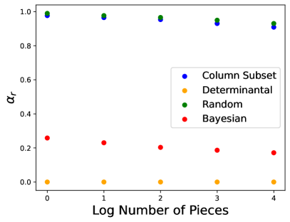
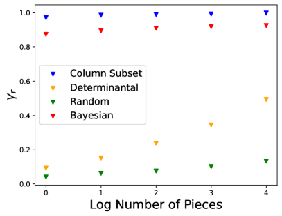
Figure 7: Shown are (a) $\alpha_{r}$ and (b) $\gamma_{r}$ for the four different function types for splitting into $1$, $2$, $4$, $8$, and $16$ pieces.

G.3 Low Elementary Rank Approximations

Here we let $n=7$. We sampled 50 different sample functions for each function and then computed the low elementary rank approximation for $r+1=1,2,3,4,5,6,7$. Appendix E.1 discusses the details of the algorithm used to compute the low-rank approximations.

Determinantal.

Here we first sample $X\in\mathbb{R}^{n\times 2n}$ with i.i.d. standard Gaussian entries. We then form $\Sigma=XX^{T}$. We also set $\sigma=0.1$.

Bayesian A-optimality.

Here we first sample $X\in\mathbb{R}^{60\times n}$ with i.i.d. standard Gaussian entries. We use $\beta=1$ and $\sigma=0.01$

Column subset.

Here we first sample $A\in\mathbb{R}^{60\times n}$ with i.i.d. standard Gaussian entries.

Random.

There are no hyperparameters to set.

G.4 r-Split Greedy with small $n$

Here we let $n=20$. We sampled 50 different sample functions for each function and for each function, ran Greedy and r-Split with Greedy as the subroutine and $r=1,2,3$.

Determinantal.

Here we sample $X\in\mathbb{R}^{n\times 2n}$ with i.i.d. standard Gaussian entries. We then form $\Sigma=XX^{T}$. We also set $\sigma=0.1$.

Bayesian A-optimality.

Here we first sample $X\in\mathbb{R}^{60\times n}$ with i.i.d. standard Gaussian entries. We use $\beta=1$ and $\sigma=0.01$

Column subset.

Here we sample $A\in\mathbb{R}^{40\times n}$ with i.i.d. standard Gaussian entries.

Random.

There are no hyperparameters to set.

G.5 r-Split Greedy with large $n$

Here we let $n=25,50,75,100,150,200,250,300,350,400,450,500$. We sampled five different sample functions for each function and, for each function, ran Greedy and r-Split with Greedy as the subroutine and $r=1$.

Determinantal.

Here we first sample $X\in\mathbb{R}^{n\times n}$ with i.i.d. standard Gaussian entries. We then form $\Sigma=XX^{T}$. We also set $\sigma=1$.

Bayesian A-optimality.

Here we first sample $X\in\mathbb{R}^{60\times n}$ with i.i.d. standard Gaussian entries. We use $\beta=0.1$ and $\sigma=0.1$

Column subset.

We use MNIST dataset for this problem.

G.6 Initial Seed Greedy

To compare algorithms with the same time dependence on $n$, we compare against a method we term Initial Seed Greedy. This algorithm provides an initial set to Greedy. That is, instead of starting at the empty set, it starts at a provided set. We then compare Initial Seed Greedy by providing all $\binom{n}{r}$ seeds and compare to r-split Greedy.

For $r=1$ and the Determinantal Function, we ran 100 trials for $n=25,50,75$,$100,150,200$. We saw that the two methods returned the same solution for each $n$ for most trials. However, for each $n$, for 2 to 5 trials, r-split Greedy outperformed Initial Greedy and found solutions that were between 0.3% and 7% better.

G.7 Computer and Software Infrastructure

We run all our experiments on Google Colab using libraries Pytorch, Numpy, and Itertools, which are available under licenses Caffe2, BSD, and CCA. Computer code for our algorithms and experiments is provided in https://anonymous.4open.science/r/Submodular-Set-Function-Optimization-8B0E/README.md.

Appendix H Details on Computing Volumes

The suprmodular rank $r$ functions on $\{0,1\}^{n}$ are a union of polyhedral cones in $\mathbb{R}^{2^{[n]}}$. We estimate their relative volume. We list the inequalities for each of the Minkowski sums of supermodular cones. We then sample $500{,}000$ random points from a standard Gaussian, test how many of the points live in the union of the cones, and report the percentage. Table 1 shows these estimates. We see that the volume of the cones decreases with the number of variables $n$ and increases rapidly with the rank $r$. For instance, when $n=4$ the volume of the set of submodular rank-$2$ functions, 5.9%, is nearly $1000$ times larger than the volume of the set of submodular rank-$1$ functions, 0.0072%.

One may wonder if it is possible to obtain a closed form formula for these volumes. The relative volume, or solid angle, of a cone $C\subseteq\mathbb{R}^{d}$ is defined by

$$\operatorname{Vol}(C):=\int_{C\cap B}d\mu(x)/\int_{B}d\mu(x),$$

where $B=\{x\in\mathbb{R}^{d}\colon\|x\|\leq 1\}$ is the unit ball. In general there are no closed form formulas available for such integrals, even when $C$ is polyhedral. For simplicial cones there exist Taylor series expansions that, under suitable conditions, can be evaluated to a desired truncation level [43]. Instead of triangulating the cone of functions of bounded supermodular rank and then approximating the volumes of the simplicial components via a truncation of their Taylor series, we found it more reliable to approximate the solid angle by sampling. In our computations described in the first paragraph, we use

$$\operatorname{Vol}(C)=\int_{C}p(x)d\mu(x)\approx\frac{1}{N}\sum_{i=1}^{N}\chi_{C}(x_{i}),$$

where $C$ is the cone of interest (e.g., the cone of supermodular rank-$r$ functions), $\chi_{C}$ is the indicator function of the cone, $p$ is the probability density function of a zero centered isotropic Gaussian random variable and $x_{i}$, $i=1,\ldots,N$ is a random sample thereof. To evaluate $\chi_{C}(x)$ we check if $x$ satisfies the facet-defining inequalities of any of the Minkowski sums that make up the cone, described in Theorem 8.

Upper bound on the volume of the supermodular cone.

We use the correspondence in Proposition 22 to upper bound the volume of the supermodular cone on $n$ variables, as follows. There are $2^{n-1}$ distinct $\pi$-supermodular cones, all of the same volume and with disjoint interiors. Hence the volume of $\mathcal{L}_{(1,\ldots,1)}$ is upper bounded by $2^{-n+1}$, which decreases with linear rate as $n$ increases. We show that the volume decreases at least with quadratic rate.

Proposition 71.

The relative volume of $\mathcal{L}_{(1,\ldots,1)}\subseteq\mathbb{R}^{\{0,1\}^{n}}$ is bounded above by $0.85^{2^{n}}$. In particular, it decreases at least with quadratic rate as $n$ increases.

Proof.

We define $\mathcal{L}_{0}^{(n)}:=\mathcal{L}_{(1,\ldots,1)}$ and denote the $i^{th}$ elementary supermodular cone on $n$ variables by $\mathcal{L}_{i}^{(n)}$. For distinct $i_{1},\ldots,i_{r}\in[n]$, the cones $\mathcal{L}_{0}^{(n)},\mathcal{L}_{i_{1}}^{(n)},\ldots,\mathcal{L}_{i_{r}}^{(n)}$ have the same volume and disjoint interiors, and thus

$$(r+1)\operatorname{Vol}(\mathcal{L}_{0}^{(n)})\leq\operatorname{Vol}(\mathcal{L}_{0}^{(n)}+\mathcal{L}_{i_{1}}^{(n)}+\cdots+\mathcal{L}_{i_{r}}^{(n)}).$$

A function $f$ in $\mathcal{L}_{0}^{(n)}+\mathcal{L}_{i_{1}}^{(n)}+\cdots+\mathcal{L}_{i_{r}}^{(n)}$ consists of $2^{r}$ supermodular pieces on $n-r$ variables. That is, each pieces $f$ lies in $\mathcal{L}_{0}^{(n-r)}$. Thus $f$ lives in a Cartesian product of $2^{r}$ cones $\mathcal{L}_{0}^{(n-r)}$. Conversely, a function $f$ that lives in this product of cones lies in the Minkowski sum $\mathcal{L}_{0}^{(n)}+\mathcal{L}_{i_{1}}^{(n)}+\cdots+\mathcal{L}_{i_{r}}^{(n)}$. Hence

$$\operatorname{Vol}(\mathcal{L}_{0}^{(n)}+\mathcal{L}_{i_{1}}^{(n)}+\cdots+\mathcal{L}_{i_{r}}^{(n)})=\operatorname{Vol}(\mathcal{L}_{0}^{(n-r)})^{2^{r}}.$$

Taking $r=n-2$, and noting that $\mathcal{L}_{0}^{(2)}=\frac{1}{2}$, we obtain

$$\operatorname{Vol}(\mathcal{L}_{0}^{(n)})\leq\frac{2^{-2^{n-2}}}{n-1}\leq 0.85^{2^{n}},\quad n\geq 2.$$ (5)

In particular, the relative volume of $\mathcal{L}_{(1,\ldots,1)}\subseteq\mathbb{R}^{2^{[n]}}$ decreases at least with quadratic rate. ∎

Although equation 5 significantly improves the trivial upper bound, it is not clear how tight it is. For $n=2$, the expression $\frac{2^{-2^{n-2}}}{n-1}$ in equation 5 equals 50%, which agrees with the true volume of $\mathcal{L}_{0}^{(2)}$. However, for $n=3$ and $n=4$ the values 12.5% and 2.1% it provides are larger than the experimentally obtained 3% and 0.0006% reported in Table 1. Nonetheless, the result shows that the relative volume of supermodular functions is tiny in high dimensions. This provides additional support and motivation to study relaxations of supermodularity such as our supermodular rank.

We are not aware of other works discussing the relative volume of supermodular cones. Following the above discussion, we may pose the following question:

Problem 72.

What is the relative volume of the cone of supermodular functions on $2^{[n]}$ in $\mathbb{R}^{2^{[n]}}$, and what is the asymptotic behavior of this relative volume as $n$ increases?

Appendix I Relations of Supermodular Rank and Probability Models

Probabilistic graphical models are defined by imposing conditional independence relations between the variables that are encoded by a graph, see [30]. Supermodularity (in)equalities arise naturally in probabilistic graphical models. We briefly describe these connections. We consider finite-valued random variables, denoted $X_{i}$, which take values denoted by lower case letters $x_{i}$.

Conditional independence and modularity.

Two random variables $X_{1}$ and $X_{2}$ are conditionally independent given a third variable $X_{3}$ if, for any fixed value $x_{3}$ that occurs with positive probability, the matrix of conditional joint probabilities $p(x_{1},x_{2}|x_{3})=p(x_{1},x_{2},x_{3})/p(x_{3})$ factorizes as a product of two vectors of conditional marginal probabilities,

$$p(x_{1},x_{2}|x_{3})=p(x_{1}|x_{3})p(x_{2}|x_{3}),$$

for all $x_{1}$ in the range of values of $X_{1}$ and $x_{2}$ in the range of values of $X_{2}$. This means that the matrix of conditional joint probabilities has rank one, or, equivalently, that its $2\times 2$ minors vanish. The vanishing of the $2\times 2$ minors is the requirement that any submatrix obtained by looking at two rows and two columns has determinant zero,

$$p(x_{1},x_{2}|x_{3})p(x^{\prime}_{1},x^{\prime}_{2}|x_{3})-p(x_{1},x^{\prime}_{2}|x_{3})p(x^{\prime}_{1},x_{2}|x_{3})=0,$$

for any two rows $x_{1},x^{\prime}_{1}$ and any two columns $x_{2},x^{\prime}_{2}$. Inserting the definition of conditional probabilities $p(x_{1},x_{2}|x_{3})=p(x_{1},x_{2},x_{3})/p(x_{3})$, moving the negative term to the right hand side, multiplying both sides by $p(x_{3})p(x_{3})$ and taking the logarithm, the rank one condition is rewritten in terms of log probabilities as

$$\log p(x_{1},x_{2},x_{3})+\log p(x^{\prime}_{1},x^{\prime}_{2},x_{3})=\log p(x_{1},x^{\prime}_{2},x_{3})+\log p(x^{\prime}_{1},x_{2},x_{3}),$$

for all $x_{1},x_{1}^{\prime}$ in the range of values of $X_{1}$, all $x_{2},x_{2}^{\prime}$ in the range of values of $X_{2}$, and all $x_{3}$ in the range of values of $X_{3}$. Thus, with an appropriate partial order on the sample space, a conditional independence statement corresponds to modularity equations for log probabilities.

Latent variables and supermodularity.

If some of the random variables are hidden (or latent), characterizing the visible marginals in terms of (in)equality relations between visible margins becomes a challenging problem [19, 2, 55, 35, 41, 16, 45, see, e.g.,]. In several known cases, such descriptions involve conditional independence inequalities that correspond to submodularity or supermodularity inequalities of log probabilities.

[2] studied $n$ discrete visible variables that are conditionally independent given a binary hidden variable. This is known as the $2$-mixture of a $n$-variable independence model, and denoted by $\mathcal{M}_{n,2}$. The article [2] shows that the visible marginals of $\mathcal{M}_{n,2}$ are characterized by the vanishing of certain $3\times 3$ minors (these are equalities) and conditional independence inequality relations that impose that the log probabilities are $\pi$-supermodular for some partial order $\pi$. Thus, the set of log probabilities defined by inequalities of $\mathcal{M}_{n,2}$, discarding the equalities, gives a union of $\pi$-supermodular cones.

Restricted Boltzmann machines and sums of supermodular cones.

A prominent graphical model is the restricted Boltzmann machine (RBM) [46, 24]. The model $\operatorname{RBM}_{n,\ell}$ has $n$ visible and $\ell$ hidden variables, and defines the probability distributions of $n$ visible variables that are the Hadamard (entrywise) products of any $\ell$ probability distributions belonging to $\mathcal{M}_{n,2}$. Characterizing the visible marginals represented by this model has been a topic of interest, see for instance [31, 38, 32]. In particular, [13, 34] studied the dimension of this model, and [35, 36] investigated certain inequalities satisfied by the visible marginals.

[45] obtained a full description of the $\operatorname{RBM}_{3,2}$ model. In this case there are no equations, and the set of visible log probabilities is the union of Minkowski sums of pairs of $\pi$-supermodular cones. They proposed that one could study RBMs more generally in terms of inequalities and, to this end, proposed to study the Minkowski sums of $\pi$-supermodular cones, which remained an open problem in their work. We have provided a characterization of these sums in Theorem 8.

Proposition 43 implies that the model $\operatorname{RBM}_{n,\ell}$ is not a universal approximator whenever $\ell<\lceil\log_{2}n\rceil+1$. This does not give new non-trivial bounds for the minimum size of a universal approximator for $n\geq 4$, since the number of parameters of the model, $(n+1)(\ell+1)-1$, is smaller than the dimension of the space, $2^{n}-1$. However, the result shows that any probability distributions on $\{0,1\}^{n}$ whose logarithm is in the interior of the submodular cone requires at least $\ell=\lceil\log_{2}(n)\rceil$ to lie in $\operatorname{RBM}_{n,\ell}$. This complements previous results based on polyhedral sets called mode poset probability polytopes [35, 37].

References

- [1] Alexander A. Ageev and Maxim Sviridenko “Pipage rounding: A new method of constructing algorithms with proven performance guarantee” In Journal of Combinatorial Optimization 8, 2004, pp. 307–328
- [2] Elizabeth S. Allman, John A. Rhodes, Bernd Sturmfels and Piotr Zwiernik “Tensors of nonnegative rank two” Special issue on Statistics In Linear Algebra and its Applications 473, 2015, pp. 37–53 URL: https://www.sciencedirect.com/science/article/pii/S0024379513006812
- [3] Benjamin Assarf, Ewgenij Gawrilow, Katrin Herr, Michael Joswig, Benjamin Lorenz, Andreas Paffenholz and Thomas Rehn “Computing convex hulls and counting integer points with Polymake” In Mathematical Programming Computation 9.1, 2017, pp. 1–38 URL: https://doi.org/10.1007/s12532-016-0104-z
- [4] Wenruo Bai, Rishabh Iyer, Kai Wei and Jeff Bilmes “Algorithms for optimizing the ratio of submodular functions” In Proceedings of The 33rd International Conference on Machine Learning 48, Proceedings of Machine Learning Research New York, New York, USA: PMLR, 2016, pp. 2751–2759 URL: https://proceedings.mlr.press/v48/baib16.html
- [5] Andrew An Bian, Joachim M Buhmann, Andreas Krause and Sebastian Tschiatschek “Guarantees for greedy maximization of non-submodular functions with applications” In International conference on machine learning, 2017, pp. 498–507 PMLR
- [6] Ilija Bogunovic, Junyao Zhao and Volkan Cevher “Robust maximization of non-submodular objectives” In Proceedings of the Twenty-First International Conference on Artificial Intelligence and Statistics 84, Proceedings of Machine Learning Research PMLR, 2018, pp. 890–899 URL: https://proceedings.mlr.press/v84/bogunovic18a.html
- [7] Yuri Boykov and Vladimir Kolmogorov “An experimental comparison of min-cut/max-flow algorithms for energy minimization in vision” In IEEE Transactions on Pattern Analysis and Machine Intelligence 26.9, 2004, pp. 1124–1137
- [8] Justin Brickell, Inderjit S. Dhillon, Suvrit Sra and Joel A. Tropp “The metric nearness problem” In SIAM Journal on Matrix Analysis and Applications, 2008
- [9] Niv Buchbinder, Moran Feldman, Joseph (Seffi) Naor and Roy Schwartz “Submodular maximization with cardinality constraints”, SODA ’14 Portland, Oregon: Society for IndustrialApplied Mathematics, 2014, pp. 1433–1452
- [10] Gruia Călinescu, Chandra Chekuri, Martin Pál and Jan Vondrák “Maximizing a monotone submodular function subject to a matroid constraint” In SIAM J. Comput. 40, 2011, pp. 1740–1766
- [11] Lin Chen, Moran Feldman and Amin Karbasi “Weakly submodular maximization beyond cardinality constraints: does randomization help greedy?” In International Conference on Machine Learning, 2018, pp. 804–813 PMLR
- [12] Michele Conforti and Gérard Cornuéjols “Submodular set functions, matroids and the greedy algorithm: tight worst-case bounds and some generalizations of the rado-edmonds theorem” In Discrete Applied Mathematics 7.3, 1984, pp. 251–274 URL: https://www.sciencedirect.com/science/article/pii/0166218X84900039
- [13] Maria Angélica Cueto, Jason Morton and Bernd Sturmfels “Geometry of the restricted Boltzmann machine” In Algebraic methods in statistics and probability : volume 2 516, Contemporary mathematics Providence, R.I.: American Mathematical Society, 2010, pp. 135–153
- [14] Abhimanyu Das and David Kempe “Submodular meets spectral: Greedy algorithms for subset selection, sparse approximation and dictionary Selection” In Proceedings of the 28th International Conference on International Conference on Machine Learning, 2011, pp. 1057–1064
- [15] Ding-Zhu Du, Ronald L. Graham, Panos M. Pardalos, Peng-Jun Wan, Weili Wu and Wenbo Zhao “Analysis of greedy approximations with non-submodular potential functions” In Proceedings of the Nineteenth Annual ACM-SIAM Symposium on Discrete Algorithms, SODA ’08 San Francisco, California: Society for IndustrialApplied Mathematics, 2008, pp. 167–175
- [16] Robin J. Evans “Margins of discrete Bayesian networks” In The Annals of Statistics 46.6A Institute of Mathematical Statistics, 2018, pp. 2623–2656 URL: https://doi.org/10.1214/17-AOS1631
- [17] Chenglin Fan, Anna C. Gilbert, Benjamin Raichel, Rishi Sonthalia and Gregory Van Buskirk “Generalized metric repair on graphs” In 17th Scandinavian Symposium and Workshops on Algorithm Theory (SWAT 2020), 2020
- [18] Yuval Filmus and Justin Ward “A tight combinatorial algorithm for submodular maximization subject to a matroid constraint” In 2012 IEEE 53rd Annual Symposium on Foundations of Computer Science, 2012, pp. 659–668 IEEE
- [19] Luis David Garcia, Michael Stillman and Bernd Sturmfels “Algebraic geometry of Bayesian networks” Special issue on the occasion of MEGA 2003 In Journal of Symbolic Computation 39.3, 2005, pp. 331–355 URL: https://www.sciencedirect.com/science/article/pii/S0747717105000076
- [20] Khashayar Gatmiry and Manuel Gomez-Rodriguez “Non-submodular function maximization subject to a matroid constraint, with applications” See also “The Network Visibility Problem”, ACM Transactions on Information Systems, Volume 40, Issue 2, Article No.: 22, pp 1–42, 2021 In arXiv preprint arXiv:1811.07863, 2018
- [21] Ewgenij Gawrilow and Michael Joswig “Polymake: A framework for analyzing convex polytopes” In Polytopes — Combinatorics and Computation Basel: Birkhäuser Basel, 2000, pp. 43–73 URL: https://doi.org/10.1007/978-3-0348-8438-9_2
- [22] Anna C. Gilbert and Rishi Sonthalia “Unsupervised metric learning in presence of missing data” In 56th Annual Allerton Conference on Communication, Control, and Computing (Allerton 2018), 2018
- [23] Marwa El Halabi and Stefanie Jegelka “Optimal approximation for unconstrained non-submodular minimization” In Proceedings of the 37th International Conference on Machine Learning 119, Proceedings of Machine Learning Research PMLR, 2020, pp. 3961–3972 URL: https://proceedings.mlr.press/v119/halabi20a.html
- [24] Geoffrey E. Hinton “Training products of experts by minimizing contrastive divergence” In Neural Comput. 14.8 Cambridge, MA, USA: MIT Press, 2002, pp. 1771–1800 URL: https://doi.org/10.1162/089976602760128018
- [25] Thibaut Horel and Yaron Singer “Maximization of approximately submodular functions” In Advances in Neural Information Processing Systems 29 Curran Associates, Inc., 2016 URL: https://proceedings.neurips.cc/paper/2016/file/81c8727c62e800be708dbf37c4695dff-Paper.pdf
- [26] Takuya Kashimura, Tomonari Sei, Akimichi Takemura and Kentaro Tanaka “Cones of elementary imsets and supermodular functions: A review and some new results”, Mathematical engineering technical reports Department of Mathematical Informatics Graduate School of Information ScienceTechnology the University of Tokyo, 2011 URL: https://books.google.com/books?id=JkrMlgEACAAJ
- [27] Andreas Krause, Ajit Singh and Carlos Guestrin “Near-optimal sensor placements in Gaussian processes: Theory, efficient algorithms and empirical studies” In Journal of Machine Learning Research 9.8, 2008, pp. 235–284 URL: http://jmlr.org/papers/v9/krause08a.html
- [28] Jeroen Kuipers, Dries Vermeulen and Mark Voorneveld “A generalization of the Shapley–Ichiishi result” In International Journal of Game Theory 39 Springer, 2010, pp. 585–602
- [29] Alex Kulesza and Ben Taskar “Determinantal point processes for machine learning” Hanover, MA, USA: Now Publishers Inc., 2012
- [30] Steffen L. Lauritzen “Graphical Models”, Oxford Statistical Sci. Ser. Oxford: Clarendon Press, 1996
- [31] Nicolas Le Roux and Yoshua Bengio “Representational power of restricted Boltzmann machines and deep belief networks” In Neural Computation 20.6, 2008, pp. 1631–1649
- [32] James Martens, Arkadev Chattopadhya, Toni Pitassi and Richard Zemel “On the representational efficiency of restricted Boltzmann machines” In Advances in Neural Information Processing Systems 26 Curran Associates, Inc., 2013 URL: https://proceedings.neurips.cc/paper_files/paper/2013/file/7bb060764a818184ebb1cc0d43d382aa-Paper.pdf
- [33] František Matúš “Conditional independences among four random variables III: Final conclusion” In Combinatorics, Probability and Computing 8.3 Cambridge University Press, 1999, pp. 269–276
- [34] Guido Montúfar and Jason Morton “Dimension of marginals of Kronecker product models” In SIAM Journal on Applied Algebra and Geometry 1.1, 2017, pp. 126–151 URL: https://doi.org/10.1137/16M1077489
- [35] Guido Montúfar and Jason Morton “When does a mixture of products contain a product of mixtures?” In SIAM Journal on Discrete Mathematics 29.1, 2015, pp. 321–347 URL: https://doi.org/10.1137/140957081
- [36] Guido Montúfar and Johannes Rauh “Hierarchical models as marginals of hierarchical models” In International Journal of Approximate Reasoning 88, 2017, pp. 531–546 URL: https://www.sciencedirect.com/science/article/pii/S0888613X16301414
- [37] Guido Montúfar and Johannes Rauh “Mode poset probability polytopes” In Journal of Algebraic Statistics 7.21, 2016, pp. 1–13
- [38] Guido Montúfar, Johannes Rauh and Nihat Ay “Expressive power and approximation errors of restricted Boltzmann machines” In Advances in Neural Information Processing Systems 24 Curran Associates, Inc., 2011 URL: https://proceedings.neurips.cc/paper_files/paper/2011/file/8e98d81f8217304975ccb23337bb5761-Paper.pdf
- [39] Mukund Narasimhan, Nebojsa Jojic and Jeff A Bilmes “Q-Clustering” In Advances in Neural Information Processing Systems 18 MIT Press, 2005 URL: https://proceedings.neurips.cc/paper_files/paper/2005/file/b0bef4c9a6e50d43880191492d4fc827-Paper.pdf
- [40] George L. Nemhauser, Laurence A. Wolsey and Marshall L. Fisher “An analysis of approximations for maximizing submodular set functions–I” In Mathematical Programming 14, 1978, pp. 265–294
- [41] Yang Qi, Pierre Comon and Lek-Heng Lim “Semialgebraic geometry of nonnegative tensor rank” In SIAM Journal on Matrix Analysis and Applications 37.4, 2016, pp. 1556–1580 URL: https://doi.org/10.1137/16M1063708
- [42] Chao Qian, Jing-Cheng Shi, Yang Yu, Ke Tang and Zhi-Hua Zhou “Optimizing ratio of monotone set functions” In Proceedings of the 26th International Joint Conference on Artificial Intelligence, IJCAI’17 Melbourne, Australia: AAAI Press, 2017, pp. 2606–2612
- [43] Jason M. Ribando “Measuring solid angles beyond dimension three” In Discrete & Computational Geometry 36.3, 2006, pp. 479–487 URL: https://doi.org/10.1007/s00454-006-1253-4
- [44] William A. Stein “Sage Mathematics Software (Version 9.4)” http://www.sagemath.org, 2023 The Sage Development Team
- [45] Anna Seigal and Guido Montúfar “Mixtures and products in two graphical models” In Journal of Algebraic Statistics, 2018
- [46] Paul Smolensky “Information processing in dynamical systems: foundations of harmony theory” In Symposium on Parallel and Distributed Processing MIT Press, 1986, pp. 194–281
- [47] Le Song, Alex Smola, Arthur Gretton, Justin Bedo and Karsten Borgwardt “Feature selection via dependence maximization” In Journal of Machine Learning Research 13.47, 2012, pp. 1393–1434 URL: http://jmlr.org/papers/v13/song12a.html
- [48] Rishi Sonthalia and Anna C. Gilbert “Project and Forget: Solving large-scale metric constrained problems” In Journal of Machine Learning Research 23.326, 2022, pp. 1–54 URL: http://jmlr.org/papers/v23/20-1424.html
- [49] Milan Studený “Basic facts concerning extreme supermodular functions” In arXiv:1612.06599, 2016
- [50] Milan Studený “On mathematical description of probabilistic conditional independence structures”, 2001 URL: http://ftp.utia.cas.cz/pub/staff/studeny/ms-doktor-01-pdf.pdf
- [51] Milan Studený “Probabilistic conditional ondependence structures” Springer Publishing Company, Incorporated, 2010
- [52] Maxim Sviridenko, Jan Vondrák and Justin Ward “Optimal approximation for submodular and supermodular optimization with bounded curvature” In Mathematics of Operations Research 42.4 INFORMS, 2017, pp. 1197–1218
- [53] Yijing Wang, Dachuan Xu, Yanjun Jiang and Dongmei Zhang “Minimizing ratio of monotone non-submodular functions” In Journal of the Operations Research Society of China, 2019, pp. 1–11
- [54] Kai Wei, Rishabh Iyer and Jeff Bilmes “Submodularity in data subset selection and active learning” In Proceedings of the 32nd International Conference on Machine Learning 37, Proceedings of Machine Learning Research Lille, France: PMLR, 2015, pp. 1954–1963 URL: https://proceedings.mlr.press/v37/wei15.html
- [55] Piotr Zwiernik “Semialgebraic statistics and latent tree models” ChapmanHall/CRC, 2015