Automated Market Making and Arbitrage Profits
in the Presence of Fees

Abstract

We consider the impact of trading fees on the profits of arbitrageurs trading against an automated marker marker (AMM) or, equivalently, on the adverse selection incurred by liquidity providers due to arbitrage. We extend the model of Milionis et al. (2022) for a general class of two asset AMMs to both introduce fees and discrete Poisson block generation times. In our setting, we are able to compute the expected instantaneous rate of arbitrage profit in closed form. When the fees are low, in the fast block asymptotic regime, the impact of fees takes a particularly simple form: fees simply scale down arbitrage profits by the fraction of time that an arriving arbitrageur finds a profitable trade.

1 Introduction

For automated market makers (AMMs), the primary cost incurred by liquidity providers (LPs) is adverse selection. Adverse selection arises from the fact that agents (‘‘arbitrageurs’’) with an informational advantage, in the form of knowledge of current market prices, can exploit stale prices on the AMM versus prices on other markets such as centralized exchanges. Because trades between arbitrageurs and the AMM are zero sum, any arbitrage profits will be realized as losses to the AMM LPs. Milionis et al. (2022) quantify these costs through a metric called loss-versus-rebalancing ($\mathsf{LVR}$). They establish that $\mathsf{LVR}$ can be simultaneously interpreted as: (1) arbitrage profits due to stale AMM prices; (2) the loss incurred by LPs relative to a trading strategy (the ‘‘rebalancing strategy’’) that holds the same risky positions as the pool, but that trades at market prices rather than AMM prices; and (3) the value of the lost optionality when an LP commits upfront to a particular liquidity demand curve. They develop formulas for $\mathsf{LVR}$ in closed form, and show theoretically and empirically that, once market risk is hedged, the profit-and-loss ($\mathsf{P\&L}$) of an LP reduces to trading fee income minus $\mathsf{LVR}$. In this way, $\mathsf{LVR}$ isolates the costs of liquidity provision.

Despite its benefits, $\mathsf{LVR}$ suffers from a significant flaw: it is derived under the simplification that arbitrageurs do not pay trading fees. In practice, however, trading fees pose a significant friction and limit arbitrage profits. The main contribution of the present work is to develop a tractable model for arbitrage profits in the presence of trading fees. We are able to obtain general formulas for arbitrageur profits in this setting. We establish that arbitrage profits in the presence of fees are roughly equivalent to the arbitrage profits in the frictionless case (i.e., $\mathsf{LVR}$), but scaled down to adjust for the fraction of time where the AMM price differs from the market price significantly enough that arbitrageurs can make profits even in the presence of fees. That is, the introduction of fees can be viewed as a rescaling of time.

Our goal is to introduce fees and understand how they impact arbitrageur behavior. As a starting point, one could directly introduce fees into the model of Milionis et al. (2022), where prices follow a geometric Brownian motion and arbitrageurs continuously monitor the AMM. However, this approach suffers a major pathology: when arbitrageurs monitor the market continuously in the presence of even negligible non-zero fees, the arbitrage profits are zero! Intuitively, when there are no fees, every instantaneous price movement provides a profitable arbitrage opportunity. With fees, this is true only for movements outside a (fee-dependent) ‘‘no-trade region’’ around the AMM price which, with continuous monitoring, then results in an immediate repositioning of that region. One can show that the fraction of time for which this happens is zero, with the market price inside the no-trade region at all other times. This is analogous to the fact that, in continuous time, a reflected random walk spends almost none of its time at the boundaries. In reality, however, arbitrageurs cannot continuously monitor and trade against the AMM. For example, for an AMM implemented on a blockchain, the arbitrageurs can only act at the discrete times at which blocks are generated. Thus, in order to understand arbitrage profits in the presence of fees, it is critical to model the discreteness of block generation.

1.1 Model

Our starting point is the model of Milionis et al. (2022), where arbitrageurs continuously monitor an AMM to trade a risky asset versus the numéraire, and the risky asset price follows geometric Brownian motion parameterized by volatility $\sigma>0$. However, we assume that the AMM has a trading fee $\gamma\geq 0$, and that arbitrageurs arrive to trade on the AMM at discrete times according to the arrivals of a Poisson process with rate $\lambda>0$. The Poisson process is a natural choice because of its memoryless nature and standard usage throughout continuous time finance. It is natural to assume arrival times correspond to block generation times, since the arbitrageurs can only trade at instances where block are generated, so the parameter $\lambda$ should be calibrated so that the mean interarrival time $\Delta t\triangleq\lambda^{-1}$ corresponds to the mean interblock time.

When an arbitrageur arrives, they seek to make a trade that myopically maximizes their immediate profit. Arbitrageurs trade myopically because of competition. If they choose to forgo immediate profit but instead wait for a larger mispricing, they risk losing the profitable trading opportunity to the next arbitrageur. If the AMM price net of fees is below (respectively, above) the market price, the arbitrageur will buy (sell) from the pool and sell (buy) at the market. They will do so until the net marginal price of the AMM equals the market price. We describe these dynamics in terms of a mispricing process that is the difference between the AMM and market log-prices. At each arrival time, a myopic arbitrageur will trade in a way such that the pool mispricing to jumps to the nearest point in band around zero mispricing. The width of the band is determined by the fee $\gamma$. We call this band the no-trade region, since if the arbitrageur arrives and the mispricing is already in the band, there is no profitable trade possible. At all non-arrival times, the mispricing is a diffusion, driven by the geometric Brownian motion governing market prices.

1.2 Results

In our setting, the mispricing process is a Markovian jump-diffusion process. Our first result is to establish that this process is ergodic, and to identify its steady state distribution in closed form. Under this distribution, the probability that an arbitrageur arrives and can make a profitable trade, i.e., the fraction of time that the mispricing process is outside the no-trade region in steady state, is given by

$$\mathsf{P}_{\mathsf{trade}}\triangleq\frac{1}{1+\underbrace{\sqrt{2\lambda}\gamma/\sigma}_{\triangleq\eta}}.$$

This can also be interpreted as the long run fraction of blocks that contain an arbitrage trade. $\mathsf{P}_{\mathsf{trade}}$ has intuitive structure in that it is a function of the composite parameter $\eta\triangleq\gamma/(\sigma\sqrt{\lambda^{-1}/2})$, the fee measured as a multiple of the typical (one standard deviation) movement of returns over half the average interarrival time. When $\eta$ is large (e.g., high fee, low volatility, or frequent blocks), the width of the no-fee region is large relative to typical interarrival price moves, so the mispricing process is less likely to exit the no-trade region in between arrivals, and $\mathsf{P}_{\mathsf{trade}}\approx\eta^{-1}$.

Given the steady state distribution of the pool mispricing, we can quantify the arbitrage profits. Denote by $\mathsf{ARB}_{T}$ the cumulative arbitrage profits over the time interval $[0,T]$. We compute the expected instantaneous rate of arbitrage profit $\overline{\mathsf{ARB}}\triangleq\lim_{T\rightarrow 0}\mathsf{E}[\mathsf{ARB}_{T}]/T$, where the expectation is over the steady state distribution of mispricing. We derive a semi-closed form expression (involving an expectation) for $\overline{\mathsf{ARB}}$. For specific cases, such as geometric mean or constant product market makers, this expectation can be evaluated resulting in an explicit closed form.

We further consider an asymptotic analysis in the fast block regime where $\lambda\rightarrow\infty$ (equivalently, the limit as the mean interblock time $\Delta t\triangleq\lambda^{-1}\rightarrow 0$). In order to explain our asymptotic results, we begin with the frictionless base case of Milionis et al. (2022), where there is no fee ($\gamma=0$) and continuous monitoring ($\lambda=\infty$). Milionis et al. (2022) establish that the expected instantaneous rate of arbitrage profit is

$$\overline{\mathsf{LVR}}\triangleq\lim_{T\rightarrow 0}\frac{\mathsf{E}\left[\mathsf{LVR}_{T}\right]}{T}=\frac{\sigma^{2}P}{2}\times y^{*\prime}\left(P\right).$$ (1)

Here, $P$ is the current market price, while $y^{*}(P)$ is the quantity of numéraire held by the pool when the market price is $P$, so that $y^{*\prime}(P)$ is the marginal liquidity of the pool at price $P$, denominated in the numéraire. In the presence of fees and discrete monitoring, our rigorous analysis establishes that as $\lambda\rightarrow\infty$,

$$\overline{\mathsf{ARB}}\triangleq\lim_{T\rightarrow 0}\frac{\mathsf{E}\left[\mathsf{ARB}_{T}\right]}{T}=\frac{\sigma^{2}P}{2}\times\underbrace{\frac{y^{*\prime}\left(Pe^{-\gamma}\right)+y^{*\prime}\left(Pe^{+\gamma}\right)}{2}}_{\text{$=y^{*\prime}\left(P\right)+O(\gamma^{2})$ for $\gamma$ small}}\times\underbrace{\frac{1}{1+\sqrt{2\lambda}\gamma/\sigma}}_{=\mathsf{P}_{\mathsf{trade}}}+o\left(\sqrt{\lambda^{-1}}\right).$$ (2)

Equations (1) and (2) differ in two ways. First, (1) involves the marginal liquidity $y^{*\prime}(P)$ at the current price $P$, while (2) averages the marginal liquidity at the endpoints of the no-trade interval of prices $[Pe^{-\gamma},Pe^{+\gamma}]$. This difference is minor if the fee $\gamma$ is small. The second difference, which is major, is that arbitrage profits in (2) are scaled down relative to (1) by precisely the factor $\mathsf{P}_{\mathsf{trade}}$. In other words, if the fee is low, in the fast block regime we can view the impact of the fee on arbitrage profits as scaling down $\mathsf{LVR}$ by the fraction of time that an arriving arbitrageur can profitably trade: $\overline{\mathsf{ARB}}\approx\overline{\mathsf{LVR}}\times\mathsf{P}_{\mathsf{trade}}$.

Focusing on the dependence on problem parameters, when $\gamma>0$, (2) implies that in the fast block regime arbitrage profits are proportional to the square root of the mean interblock time ($\sqrt{\lambda^{-1}})$, the cube of the volatility ($\sigma^{3}$), and the reciprocal of the fee ($\gamma^{-1}$). These scaling dependencies are consistent with the assertions and simulation results of Nezlobin (2022), who discusses a similar problem for constant product market makers and a deterministic block generation process. Equation (2) also highlights an interesting phase transition with the introduction of fees. Specifically, in the absence of fees ($\gamma=0$), in the fast block regime ($\lambda\rightarrow\infty$), we have the $\overline{\mathsf{ARB}}=\overline{\mathsf{LVR}}+o(1)=\Theta(1)$, i.e., up to a first order, arbitrage profits per unit time are constant and do not depend on the interblock time. On the other hand, when there are fees ($\gamma>0$), we have that $\overline{\mathsf{ARB}}=\Theta(\sqrt{\lambda^{-1}})$, arbitrage profits per unit time scale with the square root of the interblock time.

1.3 Conclusion

This work has broad implications around liquidity provision and the design of automated market makers. First, the model presented hereby provides a more accurate quantification of LP $\mathsf{P\&L}$, accounting both for arbitrageurs paying trading fees and discrete arbitrageur arrival times. As such, this model can be used for empirical analyses to evaluate LP performance both ex post as well as ex ante, when coupled with realized metrics of pool data, such as realized asset price volatility. Our results also have the potential to better inform AMM design, and in particular, provide guidance around how to set trading fees in a competitive LP market, in order to balance LP fee income and LP loss due to arbitrageurs. Finally, the asymptotic regime analysis $\lambda\to\infty$ above points to a significant potential mitigator of arbitrage profits: running a chain with lower mean interblock time $\Delta t\triangleq\lambda^{-1}$ (essentially, a faster chain), since we show that this effectively reduces arbitrage profit without negatively impacting LP fee income derived from noise trading.

1.4 Literature Review

There is a rich literature on constant function market makers. Angeris and Chitra (2020) and Angeris et al. (2021a, b) apply tools from convex analysis (e.g., the pool reserve value function) that we also use in this paper. In the first paper to decompose the return of an LP into an instantaneous market risk component and a non-negative, non-decreasing, and predictable component called ‘‘loss-versus-rebalancing’’ ($\mathsf{LVR}$, pronounced ‘‘lever’’), Milionis et al. (2022) analyze the frictionless, continuous-time Black-Scholes setting in the absence of trading fees to show that it is exactly the adverse selection cost due to the arbitrageurs’ informational advantage to the pool. This work extends the model of Milionis et al. (2022) to account for arbitrage profits both in the presence of fees and discrete-time arbitrageur arrivals. Evans et al. (2021) observe that, in the special case of geometric mean market makers, taking the limit to continuous time while holding the fees $\gamma>0$ fixed and strictly positive yields vanishing arbitrage profits; this is also a special case of our results. Angeris et al. (2021b) also analyze arbitrage profits, but do not otherwise express them in closed-form. Black-Scholes-style options pricing models, like the ones developed in this paper, have been applied to weighted geometric mean market makers over a finite time horizon by Evans (2020), who also observes that constant product pool values are a super-martingale because of negative convexity. Clark (2020) replicates the payoff of a constant product market over a finite time horizon in terms of a static portfolio of European put and call options. Tassy and White (2020) compute the growth rate of a constant product market maker with fees. Dewey and Newbold (2023) develop a model of pricing and hedging AMMs with arbitrageurs and noise traders and conjecture that arbitrageurs induce the same stationary distribution of mispricing that we rigorously develop here.

2 Model

Assets. Fix a filtered probability space $\big{(}\Omega,\mathcal{F},\{\mathcal{F}_{t}\}_{t\geq 0})$ satisfying the usual assumptions. Consider two assets: a risky asset $x$ and a numéraire asset $y$. Working over continuous times $t\in\mathbb{R}_{+}$, assume that there is observable external market price $P_{t}$ at each time $t$. The price $P_{t}$ evolves exogenously according to the geometric Brownian motion

$$\frac{dP_{t}}{P_{t}}=\mu\,dt+\sigma\,dB_{t},\quad\forall\ t\geq 0,$$

with drift $\mu$, volatility $\sigma>0$, and where $B_{t}$ is a Brownian motion.

AMM Pool. We assume that the AMM operates as a constant function market maker (CFMM). The state of a CFMM pool is characterized by the reserves $(x,y)\in\mathbb{R}^{2}_{+}$, which describe the current holdings of the pool in terms of the risky asset and the numéraire, respectively. Define the feasible set of reserves $\mathcal{C}$ according to

$$\mathcal{C}\triangleq\{(x,y)\in\mathbb{R}^{2}_{+}\ :\ f(x,y)=L\},$$

where $f\colon\mathbb{R}_{+}^{2}\rightarrow\mathbb{R}$ is referred to as the bonding function or invariant, and $L\in\mathbb{R}$ is a constant. In other words, the feasible set is a level set of the bonding function. The pool is defined by a smart contract which allows an agent to transition the pool reserves from the current state $(x_{0},y_{0})\in\mathcal{C}$ to any other point $(x_{1},y_{1})\in\mathcal{C}$ in the feasible set, so long as the agent contributes the difference $(x_{1}-x_{0},y_{1}-y_{0})$ into the pool, see Figure 1(a).

(a) Transitions between any two points on the bonding curve $f(x,y)=L$ are permitted, if an agent contributes the difference into the pool.

(b) The pool value optimization problem relates points on the bonding curve to supporting hyperplanes defined by prices.

Figure 1: Illustration of a CFMM.

Define the pool value function $V\colon\mathbb{R}_{+}\rightarrow\mathbb{R}_{+}$ by the optimization problem

$$\begin{array}[]{lll}V(P)\triangleq&\mathop{\mathrm{minimize}}\limits_{(x,y)\in\mathbb{R}^{2}_{+}}&Px+y\\ &\text{\rm subject to}&f(x,y)=L.\end{array}$$ (3)

The pool value function yields the value of the pool, assuming that the external market price of the risky asset is given by $P$, and that arbitrageurs can trade instantaneously trade against the pool maximizing their profits (and simultaneously minimizing the value of the pool). Geometrically, the pool value function implicitly defines a reparameterization of the pool state from primal coordinates (reserves) to dual coordinates (prices); this is illustrated in Figure 1(b).

Following Milionis et al. (2022), we assume that the pool value function satisfies:

Assumption 1.

1. An optimal solution $\big{(}x^{*}(P),y^{*}(P)\big{)}$ to the pool value optimization (3) exists for every $P\geq 0$.

2. The pool value function $V(\cdot)$ is everywhere twice continuously differentiable.

3. For all $t\geq 0$,

   $$\mathsf{E}^{\mathbb{Q}}\left[\int_{0}^{t}x^{*}(P_{s})^{2}P_{s}^{2}\,ds\right]<\infty.$$

We refer to $\big{(}x^{*}(P),y^{*}(P)\big{)}$ as the demand curves of the pool for the risky asset and numéraire, respectively. Assumption 1(i)–(ii) is a sufficient condition for the following:

Lemma 1.

For all prices $P\geq 0$, the pool value function satisfies:

1. $V(P)\geq 0$.

2. $V^{\prime}(P)=x^{*}(P)\geq 0$.

3. $V^{\prime\prime}(P)=x^{*\prime}(P)=-Py^{*\prime}(P)\leq 0$.

The proof of Lemma 1 follows from standard arguments in convex analysis; see Milionis et al. (2022) for details.

Fee Structure. Suppose that $(\Delta x,\Delta y)$ is a feasible trade permitted by the pool invariant, i.e., given initial pool reserves $(x,y)$ with $f(x,y)=L$, we have $f(x+\Delta x,y+\Delta y)=L$. We assume that an additional proportional trading fee is paid to the LPs in the pool. The mechanics of this trading fee are as follows:

1. The fee is paid in the numéraire in proportion to the quantity $\Delta y$ of numéraire that is traded.

2. The fee is realized as a separate cashflow to the LPs.

3. We allow for different fees to be paid when the risky asset is bought from the pool and when the risky asset is sold to the pool.

4. We denote the fee in units of log price by $\gamma_{+},\gamma_{-}>0$. In particular, when the agent purchases the risky asset from the pool (i.e., $\Delta x<0$, $\Delta y>0$), the total fee charged is

   $$\left\lparen e^{+\gamma_{+}}-1\right\rparen\left\lvert\Delta y\right\rvert,$$ (4)

   while the total fee charged when the agent sells the risky asset to the pool (i.e., $\Delta x>0$, $\Delta y<0$ is

   $$\left\lparen 1-e^{-\gamma_{-}}\right\rparen\left\lvert\Delta y\right\rvert.$$ (5)

Example 1.

In our notation, a 30 basis point proportional fee on either buys or sales (e.g., as in Uniswap V2) would correspond to

$$\gamma_{+}=\log(1+0.003)\approx 0.002995509,\quad\gamma_{-}=-\log(1-0.003)\approx 0.003004509.$$

To a first order, $\gamma_{+}\approx\gamma_{-}\approx 30\text{ (basis points)}$.

3 Arbitrageurs & Pool Dynamics

At any time $t\geq 0$, define $\tilde{P}_{t}$ to be the price of the risky asset implied by pool reserves, i.e., the reserves are be given by $\big{(}x^{*}(\tilde{P}_{t}),y^{*}(\tilde{P}_{t})\big{)}$. Denote by

$$z_{t}\triangleq\log P_{t}/\tilde{P}_{t},$$ (6)

the log mispricing of the pool, so that $\tilde{P}_{t}=P_{t}e^{-z_{t}}$.

We imagine that arbitrageurs arrive to trade against the pool at discrete times according to a Poisson process of rate $\lambda>0$. Here, we imagine that arbitrageurs are continuously monitoring the market, but can only trade against the pool at discrete times when blocks are generated in a blockchain. Hence, we will view the arrival process as both equivalently describing the arrival of arbitrageurs to trade or times of block generation. For a proof-of-work blockchain, Poisson block generation is a natural assumption (Nakamoto, 2008). However, modern proof-of-state blockchains typically generate blocks at deterministic times. In these cases, we will view the Poisson assumption as an approximation that is necessary for tractability. In any case, the mean interarrival time $\Delta t\triangleq\lambda^{-1}$ should be calibrated to the mean interblock time in a blockchain.

Denote the arbitrageur arrival times (or block generation times) by $0<\tau_{1}<\tau_{2}<\cdots$. When an arbitrageur arrives at time $t=\tau_{i}$, they can trade against the pool (paying the relevant trading fees) according to the pool mechanism, and simultaneously, frictionlessly trade on an external market at the price $P_{t}$. We assume that the arbitrageur will trade to myopically maximize their instantaneous trading profit. We ignore any blockchain transaction fees such as ‘‘gas’’.

The following lemma (with proof in Appendix A) characterizes the myopic behavior of the arbitrageurs in terms of the demand curves of the pool and the fee structure:

Lemma 2.

Suppose that an arbitrageur arrives at time $t=\tau_{i}$, observing external market price $P_{t}$, and implied pool price $\tilde{P}_{t^{-}}$ or, equivalently, mispricing $z_{t^{-}}$. Then, one of the following three cases applies:

1. If $P_{t}>\tilde{P}_{t^{-}}e^{+\gamma_{+}}$ or, equivalently, $z_{t^{-}}>+\gamma_{+}$, the arbitrageur can profitably buy in the pool and sell on the external market. They will do so until the pool price satisfies $\tilde{P}_{t}=P_{t}e^{-\gamma_{+}}$ or, equivalently, $z_{t}=+\gamma_{+}$. The arbitrageur profits are then

   $$P_{t}\left\{x^{*}\left(P_{t}e^{-z_{t^{-}}}\vphantom{\tilde{P}}\right)-x^{*}\left(P_{t}e^{-\gamma_{+}}\vphantom{\tilde{P}}\right)\right\}+e^{+\gamma_{+}}\left\{y^{*}\left(P_{t}e^{-z_{t^{-}}}\vphantom{\tilde{P}}\right)-y^{*}\left(P_{t}e^{-\gamma_{+}}\vphantom{\tilde{P}}\right)\right\}\geq 0.$$

2. If $P_{t}<\tilde{P}_{t^{-}}e^{-\gamma_{-}}$ or, equivalently, $z_{t^{-}}<-\gamma_{-}$, the arbitrageur can profitably sell in the pool and buy the external market. The will do so until the pool price satisfies $\tilde{P}_{t}=P_{t}e^{+\gamma_{-}}$ or, equivalently, $z_{t}=-\gamma_{-}$. The arbitrageur profits are then

   $$P_{t}\left\{x^{*}\left(P_{t}e^{-z_{t^{-}}}\vphantom{\tilde{P}}\right)-x^{*}\left(P_{t}e^{+\gamma_{-}}\vphantom{\tilde{P}}\right)\right\}+e^{-\gamma_{-}}\left\{y^{*}\left(P_{t}e^{-z_{t^{-}}}\vphantom{\tilde{P}}\right)-y^{*}\left(P_{t}e^{+\gamma_{-}}\vphantom{\tilde{P}}\right)\right\}\geq 0.$$

3. If $\tilde{P}_{t^{-}}e^{-\gamma_{-}}\leq P_{t}\leq\tilde{P}_{t^{-}}e^{+\gamma_{+}}$, then the arbitrageur makes no trade, and $\tilde{P}_{t}=\tilde{P}_{t^{-}}$ or, equivalently, $z_{t}=z_{t^{-}}$.

Considering the three cases in Lemma 2, it is easy to see that, at an arbitrageur arrival time $\tau_{i}$, the mispricing process $z_{t}$ evolves according to

$$z_{\tau_{i}}=\operatorname{bound}\big{\{}z_{\tau_{i}^{-}},-\gamma_{-},+\gamma_{+}\big{\}},$$ (7)

On the other hand, applying Itô’s lemma to (6), we have that, at other times $t>0$, process evolves according to

$$dz_{t}=\left(\mu-\tfrac{1}{2}\sigma^{2}\right)\,dt+\sigma\,dB_{t}.$$ (8)

Combining (7)–(8), for all $t\geq 0$,

$$z_{t}=\left(\mu-\tfrac{1}{2}\sigma^{2}\right)t+\sigma B_{t}+\sum_{i:\ \tau_{i}\leq t}J_{i},\qquad J_{i}\triangleq\operatorname{bound}\big{\{}z_{\tau_{i}^{-}},-\gamma_{-},+\gamma_{+}\big{\}}-z_{\tau_{i}^{-}}.$$ (9)

Therefore, the mispricing process $z_{t}$ is a Markovian jump-diffusion process. A possible sample path of this mispricing process is shown in Figure 2.

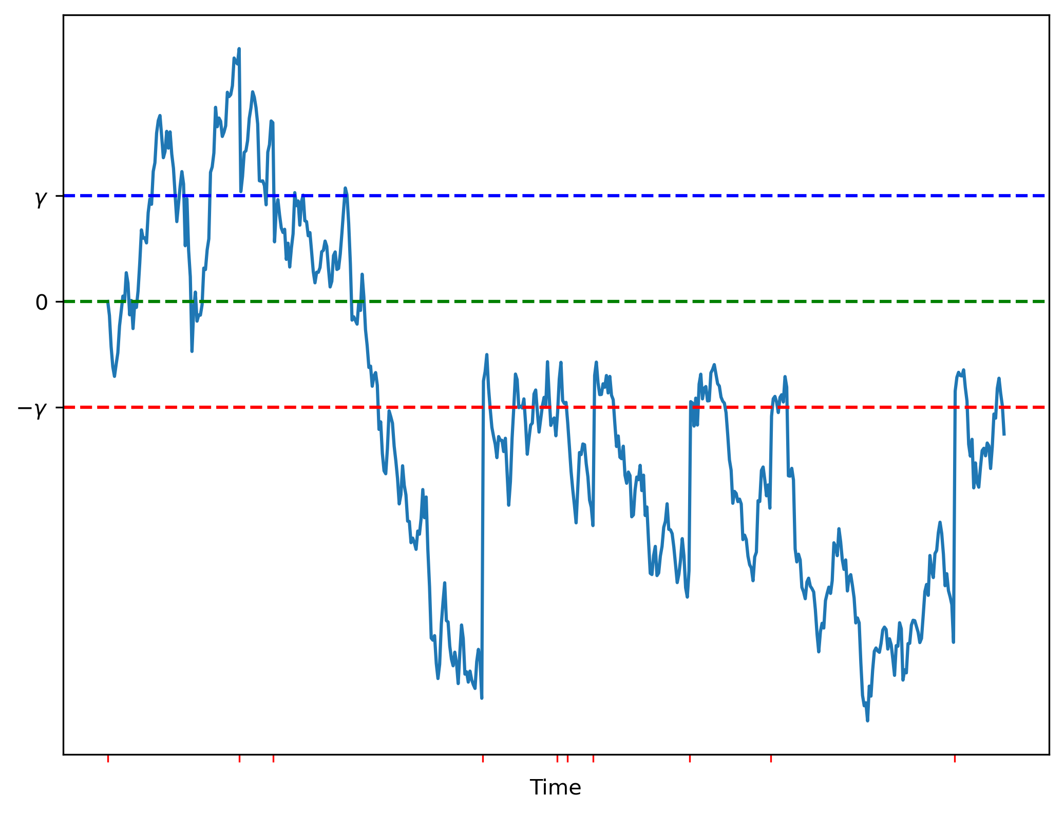
Figure 2: Example sample path of the mispricing process $z_{t}$. The red-colored ticks in the x-axis show the (Poisson-distributed) times of arbitrageur arrivals.

4 Exact Analysis

We will make the following assumption:

Assumption 2 (Symmetry).

$$\mu=\tfrac{1}{2}\sigma^{2},\qquad\gamma_{+}=\gamma_{-}\triangleq\gamma.$$

Assumption 2 ensures that the mispricing jump-diffusion process, with dynamics given by (7)–(8), is distributed symmetrically around the $z=0$ axis. This assumption will considerably simplify notation and expressions and is without loss of generality. All of our conclusions downstream can be derived without this assumption, at the expense of additional algebra. We discuss this in greater detail in Appendix C, where we also provide a non-symmetric variation of Theorem 1.

4.1 Stationary Distribution of the Mispricing Process

The following lemma characterizes the stationary distribution of the mispricing process. We defer the proof of this lemma until Appendix B.

Theorem 1 (Stationary Distribution of Mispricing).

The process $z_{t}$ is an ergodic process on $\mathbb{R}$, with unique invariant distribution $\pi(\cdot)$ given by the density

$$p_{\pi}(z)=\begin{cases}\pi_{+}\times p^{\exp}_{\eta/\gamma}(z-\gamma)&\text{if $z>+\gamma$},\\ \pi_{0}\times\frac{1}{2\gamma}&\text{if $z\in[-\gamma,+\gamma]$},\\ \pi_{-}\times p^{\exp}_{\eta/\gamma}(-\gamma-z)&\text{if $z<-\gamma$},\end{cases}$$

for $z\in\mathbb{R}$. Here, we define the composite parameter $\eta\triangleq\sqrt{2\lambda}\gamma/\sigma$. The probabilities ${\pi_{-},\pi_{0},\pi_{+}}$ of the three segments are given by

$$\pi_{0}\triangleq\pi\big{(}[-\gamma,+\gamma]\big{)}=\frac{\eta}{1+\eta},\quad\pi_{+}\triangleq\pi\big{(}(+\gamma,+\infty)\big{)}=\pi_{-}\triangleq\pi\big{(}(-\infty,-\gamma)\big{)}=\tfrac{1}{2}\frac{1}{1+\eta}.$$

Finally, $p^{\exp}_{\eta/\gamma}(x)\triangleq(\eta/\gamma)e^{-(\eta/\gamma)x}$ is the density of an exponential distribution over $x\geq 0$ with parameter $\eta/\gamma=\sqrt{2\lambda}/\sigma$.

The stationary distribution is illustrated in Figure 3.

Figure 3: The density $p_{\pi}(z)$ of the stationary distribution $\pi(\cdot)$ of mispricing $z$.

Under this distribution, the probability that an arbitrageur arrives and can make a profitable trade, i.e., the fraction of time that the mispricing process is outside the no-trade region in steady state, is given by

$$\mathsf{P}_{\mathsf{trade}}\triangleq\pi_{+}+\pi_{-}=\frac{1}{1+\sqrt{2\lambda}\gamma/\sigma}.$$

Equivalently, $\mathsf{P}_{\mathsf{trade}}$ can be interpreted as the long run fraction of blocks that contain an arbitrage trade.

Note that $\mathsf{P}_{\mathsf{trade}}$ does not depend on the bonding function or feasible set defining the CFMM pool; the only pool property relevant is the fee $\gamma$. $\mathsf{P}_{\mathsf{trade}}$ has intuitive structure in that it is a function of the composite parameter $\eta\triangleq\gamma/(\sigma\sqrt{\lambda^{-1}/2})$, the fee measured as a multiple of the typical (one standard deviation) movement of returns over half the average interarrival time. When $\eta$ is large (e.g., high fee, low volatility, or frequent blocks), the width of the no-fee region is large relative to typical interarrival price moves, so the mispricing process is less likely to exit the no-trade region in between arrivals, and $\mathsf{P}_{\mathsf{trade}}\approx\eta^{-1}$. Example calculations of $\mathsf{P}_{\mathsf{trade}}$ are shown in Table 1 for $\sigma=5\%\text{ (daily)}$ volatility and varying mean interblock times $\Delta t\triangleq\lambda^{-1}$ and fee levels $\gamma$, as well as in Figure 4(a).

$\Delta t$ \ $\gamma$	1 bp	5 bp	10 bp	30 bp	100 bp
10 min	96.7%	85.5%	74.7%	49.6%	22.8%
2 min	92.9%	72.5%	56.9%	30.5%	11.6%
12 sec	80.7%	45.6%	29.5%	12.3%	4.0%
2 sec	63.0%	25.4%	14.5%	5.4%	1.7%
50 msec	21.2%	5.1%	2.6%	0.9%	0.3%

Table 1: The probability of trade $\mathsf{P}_{\mathsf{trade}}$, or, equivalently, the fraction of blocks with contain an arbitrage trade, given asset price volatility $\sigma=5\%\text{ (daily)}$, with varying mean interblock times $\Delta t\triangleq\lambda^{-1}$ and fee levels $\gamma$ (in basis points).

(a) The probability of trade $\mathsf{P}_{\mathsf{trade}}$, or, equivalently, the fraction of blocks containing an arbitrage trade, as a function of the fee $\gamma$.

(b) The standard deviation of mispricing $\sigma_{z}$, as a function of the fee $\gamma$.

Figure 4: Probability of trade and typical mispricing errors as a function of the fee, with $\sigma=5\%\text{ (daily)}$ and mean interblock time $\Delta t\triangleq\lambda^{-1}=12\text{ (seconds)}$.

The following immediate corollary quantifies the magnitude of a typical mispricing. This is illustrated in Figure 4(b).

Corollary 1 (Standard Deviation of Mispricing).

Under the invariant distribution $\pi(\cdot)$, the standard deviation of the mispricing is given by

$$\sigma_{z}\triangleq\sqrt{\mathsf{E}_{\pi}[z^{2}]}=\sqrt{(1-\mathsf{P}_{\mathsf{trade}})\times\tfrac{1}{3}\gamma^{2}+\mathsf{P}_{\mathsf{trade}}\times\left\{\left(\gamma+\frac{\sigma}{\sqrt{2\lambda}}\right)^{2}+\frac{\sigma^{2}}{2\lambda}\right\}}.$$

4.2 Rate of Arbitrageur Profit

Denote by $N_{T}$ the total number of arbitrageur arrivals in $[0,T]$. Suppose an arbitrageur arrives at time $\tau_{i}$, observing external price $P_{\tau_{i}}$ and mispricing $z_{\tau_{i}^{-}}$. From Lemma 2, the arbitrageur profit is given by

$$A(P_{\tau_{i}},z_{\tau_{i}^{-}})\triangleq A_{+}(P_{\tau_{i}},z_{\tau_{i}^{-}})+A_{-}(P_{\tau_{i}},z_{\tau_{i}^{-}})\geq 0,$$

where we define

$$A_{+}(P,z)\triangleq\left[P\left\{x^{*}\left(Pe^{-z}\vphantom{\tilde{P}}\right)-x^{*}\left(Pe^{-\gamma}\right)\right\}+e^{+\gamma}\left\{y^{*}\left(Pe^{-z}\vphantom{\tilde{P}}\right)-y^{*}\left(Pe^{-\gamma}\right)\right\}\right]\mathbb{I}_{\left\{z>+\gamma\right\}}\geq 0,$$

$$A_{-}(P,z)\triangleq\left[P\left\{x^{*}\left(Pe^{-z}\vphantom{\tilde{P}}\right)-x^{*}\left(Pe^{+\gamma}\vphantom{\tilde{P}}\right)\right\}+e^{-\gamma}\left\{y^{*}\left(Pe^{-z}\vphantom{\tilde{P}}\right)-y^{*}\left(Pe^{+\gamma}\vphantom{\tilde{P}}\right)\right\}\right]\mathbb{I}_{\left\{z<-\gamma\right\}}\geq 0.$$

Similarly, the fees paid by the arbitrageur in this scenarios is given by

$$F(P_{\tau_{i}},z_{\tau_{i}^{-}})\triangleq F_{+}(P_{\tau_{i}},z_{\tau_{i}^{-}})+F_{-}(P_{\tau_{i}},z_{\tau_{i}^{-}})\geq 0,$$

where we define

$$F_{+}(P,z)\triangleq-\left(e^{+\gamma}-1\right)\left[y^{*}\left(Pe^{-z}\vphantom{\tilde{P}}\right)-y^{*}\left(Pe^{-\gamma}\vphantom{\tilde{P}}\right)\right]\mathbb{I}_{\left\{z>+\gamma\right\}}\geq 0,$$

$$F_{-}(P,z)\triangleq+\left(1-e^{-\gamma}\vphantom{\tilde{P}}\right)\left[y^{*}\left(Pe^{-z}\vphantom{\tilde{P}}\right)-y^{*}\left(Pe^{+\gamma}\vphantom{\tilde{P}}\right)\right]\mathbb{I}_{\left\{z<-\gamma\right\}}\geq 0.$$

We can write the total arbitrage profit and fees paid over $[0,T]$ by summing over all arbitrageurs arriving in that interval, i.e.,

$$\mathsf{ARB}_{T}\triangleq\sum_{i=1}^{N_{T}}A(P_{\tau_{i}},z_{\tau_{i}^{-}}),\quad\mathsf{FEE}_{T}\triangleq\sum_{i=1}^{N_{T}}F(P_{\tau_{i}},z_{\tau_{i}^{-}}).$$

Clearly these are non-negative and monotonically increasing processes. The following theorem characterizes their instantaneous expected rate of growth or intensity:

Theorem 2 (Rate of Arbitrage Profit and Fees).

Define the intensity, or instantaneous rate of arbitrage profit, by

$$\overline{\mathsf{ARB}}\triangleq\lim_{T\rightarrow 0}\frac{\mathsf{E}\left[\mathsf{ARB}_{T}\right]}{T}.$$

Given initial price $P_{0}=P$, and suppose that $z_{0}=z$ is distributed according to its stationary distribution $\pi(\cdot)$. Then the instantaneous rate of arbitrage profit is given by

$$\begin{split}\overline{\mathsf{ARB}}&=\lambda\mathsf{E}_{\pi}\left[A(P,z)\right]=\lambda\mathsf{P}_{\mathsf{trade}}\frac{\sqrt{2\lambda}}{\sigma}\int_{0}^{\infty}\frac{A_{+}(P,x+\gamma)+A_{-}(P,-x-\gamma)}{2}e^{-\sqrt{2\lambda}x/\sigma}\,dx.\end{split}$$

Similarly, defining the intensity of the fee process by

$$\overline{\mathsf{FEE}}\triangleq\lim_{T\rightarrow 0}\frac{\mathsf{E}\left[\mathsf{FEE}_{T}\right]}{T},$$

we have that

$$\begin{split}\overline{\mathsf{FEE}}&=\lambda\mathsf{E}_{\pi}\left[F(P,z)\right]=\lambda\mathsf{P}_{\mathsf{trade}}\frac{\sqrt{2\lambda}}{\sigma}\int_{0}^{\infty}\frac{F_{+}(P,x+\gamma)+F_{-}(P,-x-\gamma)}{2}e^{-\sqrt{2\lambda}x/\sigma}\,dx.\end{split}$$

Proof.

This result follows from standard properties of Poisson processes. The smoothing formula (e.g., Theorem 13.5.7, Brémaud, 2020) yields that, for $T>0$,

$$\mathsf{E}\left[\mathsf{ARB}_{T}\right]=\mathsf{E}\left[\sum_{i=1}^{N_{T}}A(P_{\tau_{i}},z_{\tau_{i}^{-}})\right]=\mathsf{E}\left[\int_{0}^{T}A(P_{t},z_{t^{-}})\,dN_{t}\right]=\mathsf{E}\left[\int_{0}^{T}A(P_{t},z_{t^{-}})\times\lambda\,dt\right].$$

Applying Tonelli’s theorem and the fundamental theorem of calculus,

$$\lim_{T\rightarrow 0}\frac{\mathsf{E}\left[\mathsf{ARB}_{T}\right]}{T}=\lim_{T\rightarrow 0}\frac{\lambda}{T}\int_{0}^{T}\mathsf{E}\left[A(P_{t},z_{t^{-}})\right]\,dt=\lambda\mathsf{E}\left[A(P_{0},z_{0^{-}})\right],$$

and the result then follows from Theorem 1. The same argument applies to the intensity of the fee process. ∎

4.3 Example: Constant Product Market Maker

Theorem 2 provides an exact, semi-analytic closed form expression for the rate of arbitrage profit, in terms of a certain Laplace transfrom of the functions $\{A_{\pm}(P,\cdot)\}$. This expression can be evaluated as an explicit closed form for many CFMMs. For example, consider the case of constant product market makers:

Corollary 2.

Consider a constant product market maker, with invariant $f(x,y)\triangleq\sqrt{xy}=L$. Under the assumptions of Theorem 2, the intensity per dollar value in the pool is given by

$$\frac{\overline{\mathsf{ARB}}}{V(P)} =\begin{cases}\displaystyle\frac{\sigma^{2}}{8}\times\mathsf{P}_{\mathsf{trade}}\times\frac{e^{+\gamma/2}+e^{-\gamma/2}}{2\Big{\lparen}1-\sigma^{2}/(8\lambda)\Big{\rparen}}&\text{if $\sigma^{2}/8<\lambda$,}\\ +\infty&\text{otherwise.}\end{cases}$$

where the quantities on the right side do not depend on the value of $P_{0}=P$.

The proof of Corollary 2 is deferred until Appendix D. Under the normalization of Corollary 2, where the intensity of arbitrage profits is normalized relative the pool value, the resulting quantity does not depend on the price. The same property will hold for the more general class of geometric mean market makers; this is analogous to the property that $\mathsf{LVR}$ is proportional to pool value for this class (Milionis et al., 2022).

As a comparison point, for a constant product market maker, Milionis et al. (2022) establish that

$$\overline{\mathsf{LVR}}\triangleq\lim_{T\rightarrow 0}\frac{\mathsf{E}\left[\mathsf{LVR}_{T}\right]}{T}=\frac{\sigma^{2}}{8}\times V(P),$$

so that, when $\sigma^{2}/8<\lambda$,

$$\overline{\mathsf{ARB}}=\overline{\mathsf{LVR}}\times\mathsf{P}_{\mathsf{trade}}\times\underbrace{\frac{e^{+\gamma/2}+e^{-\gamma/2}}{2}}_{\approx 1+O(\gamma^{2})}\times\underbrace{\frac{1}{1-\sigma^{2}/(8\lambda)}}_{\approx 1+O(\lambda^{-1})}.$$

Therefore, when fees are small ($\gamma\rightarrow 0$) and the block rate is high ($\lambda\rightarrow\infty$), we have the approximation

$$\overline{\mathsf{ARB}}\approx\overline{\mathsf{LVR}}\times\mathsf{P}_{\mathsf{trade}}.$$ (10)

In Figure 5(b), we see that for typical parameter values this approximation is extremely accurate, with a relative error of less that $10^{-5}$.

(a) The normalized intensity of arbitrage profit $\overline{\mathsf{ARB}}/V(P)$ as a function of the fee $\gamma$.

(b) The relative error of the approximation (10), i.e., $(\overline{\mathsf{ARB}}-\overline{\mathsf{LVR}}\times\mathsf{P}_{\mathsf{trade}})/\overline{\mathsf{ARB}}$, as a function of the fee $\gamma$.

Figure 5: The constant product market maker case, with $\sigma=5\%\text{ (daily)}$ and mean interblock time $\Delta t\triangleq\lambda^{-1}=12\text{ (seconds)}$.

5 Asymptotic Analysis

In this section, we consider a fast block regime, where $\lambda\rightarrow\infty$. In this setting, block are generated very quickly, or, equivalently, the interblock time $\Delta t\triangleq\lambda^{-1}\rightarrow 0$ is very small.

Theorem 3.

Define

$$\begin{split}\bar{A}(P,x)&\triangleq\frac{A_{+}(P,x+\gamma)+A_{-}(P,-x-\gamma)}{2}\geq 0.\end{split}$$

Assume that, for each $P>0$, $\bar{A}(P,\cdot)$ is twice continuously differentiable, and that there exists $A_{0}$ and $c$ (possibly depending on $P$) such that

$$\partial_{xx}\bar{A}(P,x)\leq A_{0}e^{cx},\quad\forall\ x\geq 0.$$ (11)

Consider the fast block regime where $\lambda\rightarrow\infty$. Then,

$$\overline{\mathsf{ARB}}=\frac{\sigma^{2}P}{2}\times\frac{y^{*\prime}\left(Pe^{-\gamma}\right)+y^{*\prime}\left(Pe^{+\gamma}\right)}{2}\times\mathsf{P}_{\mathsf{trade}}+o\left(\sqrt{\lambda^{-1}}\right).$$ (12)

Theorem 4.

Define

$$\begin{split}\bar{F}(P,x)&\triangleq\frac{F_{+}(P,x+\gamma)+F_{-}(P,-x-\gamma)}{2}\geq 0.\end{split}$$

Assume that, for each $P>0$, $\bar{F}(P,\cdot)$ is continuously differentiable, and that there exists $F_{0}$ and $c$ (possibly depending on $P$) such that

$$\partial_{x}\bar{F}(P,x)\leq F_{0}e^{cx},\quad\forall\ x\geq 0.$$ (13)

Consider the fast block regime where $\lambda\rightarrow\infty$. Then, the instantaneous rate of fees (defined similarly to Theorem 2) is

$$\overline{\mathsf{FEE}}=\frac{\sigma^{2}P}{2}\times\frac{(1-e^{-\gamma})y^{*\prime}\left(Pe^{-\gamma}\right)+(e^{+\gamma}-1)y^{*\prime}\left(Pe^{+\gamma}\right)}{2\gamma}\times\left(1-\mathsf{P}_{\mathsf{trade}}\right)+o\left(1\right).$$ (14)

The proofs of Theorems 3 and 4 are deferred to Appendix E. Equation 11 is a mild technical condition bounding the convexity of the arbitrage profit as a function of the mispricing. Theorem 3 provides theoretical justification for the discussion in Section 1.2 comparing (1)–(2): we have that, for arbitrary AMMs satisfying the technical condition of (11), $\overline{\mathsf{ARB}}\approx\overline{\mathsf{LVR}}\times\mathsf{P}_{\mathsf{trade}}$ when the fee $\gamma$ is small in the fast block regime. Additionally, for arbitrary AMMs satisfying the technical condition of (13), the instantaneous rate of fees is shown by Equation 14 to be $\overline{\mathsf{FEE}}\approx\overline{\mathsf{LVR}}\times\left(1-\mathsf{P}_{\mathsf{trade}}\right)$ when the fee $\gamma$ is small in the fast block regime. The last two results mean that, conditioned on the fee $\gamma$ being small in the fast block regime, $\overline{\mathsf{ARB}}+\overline{\mathsf{FEE}}\approx\overline{\mathsf{LVR}}$, which can be interpreted as $\overline{\mathsf{LVR}}$ being split among fees and arbitrage profits, according to $\mathsf{P}_{\mathsf{trade}}$. In particular, as the blocks become more and more frequent (for a fixed fee $\gamma$), $\overline{\mathsf{LVR}}$ switches from arbitrage profits to fees, where it is eventually consumed.

Equation (12) also highlights the dependence of arbitrage profits on the problem parameters. In the regime where volatility $\sigma$ is large, the fee $\gamma$ is small, and the block rate $\lambda$ is high, we have that $\mathsf{P}_{\mathsf{trade}}\approx\eta^{-1}=\sigma\sqrt{\lambda^{-1}/2}/\gamma$. This implies that arbitrage profits are proportional to the square root of the mean interblock time ($\sqrt{\lambda^{-1}})$, the cube of the volatility ($\sigma^{3}$), and the reciprocal of the fee ($\gamma^{-1}$).

6 Pricing Accuracy vs. Arbitrage Profits

Rao and Shah (2023) suggest a trade-off for AMM designers between pricing accuracy, measured by the standard deviation of mispricing $\sigma_{z}$, and the arbitrage profits. Setting fees that are low ensures accurate prices, but results in high arbitrage profits, while setting fees that are high has the opposite effect.

In our setting, we can crisply and analytically quantify this trade-off. Namely, the standard deviation of mispricing can be computed by Corollary 1, while the arbitrage profits can be computed by Theorem 2 (exactly) or Theorem 3 (asymptotically).

Figure 6 illustrates this trade-off for a constant product market maker, where the arbitrage profits are computed exactly using Corollary 2. This figure illustrates two bounds in the low fee regime ($\gamma\rightarrow 0$). First, as $\gamma\rightarrow 0$, $\overline{\mathsf{ARB}}/V(P)\uparrow\overline{\mathsf{LVR}}/V(P)=\sigma^{2}/8$. In this sense, $\overline{\mathsf{LVR}}$ captures the worse case loss to arbitrageurs. Second, as $\gamma\rightarrow 0$, $\sigma_{z}\downarrow\sigma\sqrt{\lambda^{-1}}$. The latter quantity is the standard deviation of log-price changes over the mean interblock time $\Delta t\triangleq\lambda^{-1}$. This is the minimal mispricing error forced by the discrete nature of the blockchain.

Figure 6: Efficient frontier between mispricing error and arbitrage profits for different choices of fees, for a constant product market maker. Here, we set $\sigma=5\%\text{ (daily)}$ and $\lambda^{-1}=12\text{ (seconds)}$. The horizontal axis is the standard deviation of the steady state pool mispricing $\sigma_{z}$. The vertical axis is the intensity per unit time of arbitrage profits per dollar value of the pool $\overline{\mathsf{ARB}}/V(P)$.

Appendix A Proof of Lemma 2

Proof of Lemma 2.

We consider Part (1), the others follow by analogy. Suppose the arbitrageur considers buying from the pool, and selling on the external market at price $P_{t}$. Then, the arbitrageur will face the optimization problem

$$\begin{array}[]{lll}\mathop{\mathrm{maximize}}\limits_{\Delta x,\Delta y}&P_{t}\Delta x-e^{+\gamma_{+}}\Delta y\\ \text{\rm subject to}&f\left(x^{*}(\tilde{P}_{t^{-}})-\Delta x,y^{*}(\tilde{P}_{t^{-}})+\Delta_{y}\right)=L,\\ &\Delta_{x},\Delta_{y}\geq 0,\end{array}$$

where $(x^{*}(\tilde{P}_{t^{-}}),y^{*}(\tilde{P}_{t^{-}}))$ are the reserves of the pool immediately prior to the arrival of the arbitrageur. Here, the decision variables $\Delta x$ describes the quantity of risky asset purchased by the arbitrageur, while $\Delta y$ is the amount of numéraire paid. Instead, we can parameterize the decision through the variables

$$x\triangleq x^{*}(\tilde{P}_{t^{-}})-\Delta x,\quad y\triangleq y^{*}(\tilde{P}_{t^{-}})+\Delta_{y},$$

which describe the post-trade reserves of the pool. Thus, we can equivalently optimize

$$\begin{array}[]{lll}\mathop{\mathrm{minimize}}\limits_{x,y}&P_{t}e^{-\gamma_{+}}x+y\\ \text{\rm subject to}&f\left(x,y\right)=L,\\ &x\leq x^{*}(\tilde{P}_{t^{-}}),\ y\geq y^{*}(\tilde{P}_{t^{-}}).\end{array}$$ (15)

Comparing to (3) and using the fact that $x^{*}(\cdot)$ is monotonically decreasing while $y^{*}(\cdot)$ is monotonically increasing, it is clear that the solution to (15) is given by

$$x=\begin{cases}x^{*}\left(\vphantom{\tilde{P}}P_{t}e^{-\gamma_{+}}\right)&\text{if $P_{t}e^{-\gamma_{+}}>\tilde{P}_{t^{-}}$},\\[2.39996pt] x^{*}\left(\tilde{P}_{t^{-}}\right)&\text{otherwise,}\end{cases}\quad y=\begin{cases}y^{*}\left(\vphantom{\tilde{P}}P_{t}e^{-\gamma_{+}}\right)&\text{if $P_{t}e^{-\gamma_{+}}>\tilde{P}_{t^{-}}$},\\[2.39996pt] y^{*}\left(\tilde{P}_{t^{-}}\right)&\text{otherwise.}\end{cases}$$

Therefore a profitable trade where the arbitrageur purchases from the pool is only possible when $P_{t}>\tilde{P}_{t^{-}}e^{+\gamma_{+}}$, and the profit is as given in Part (1). ∎

Appendix B Proof of Theorem 1

Define the infinitesimal generator $\mathcal{A}$ by

$$\mathcal{A}f(z)\triangleq\lim_{\Delta t\rightarrow 0}\frac{1}{\Delta t}\mathsf{E}\left[\left.f(z_{\Delta t})-f(z_{0})\right|z_{0}=z\right],$$

for $f\colon\mathbb{R}\rightarrow\mathbb{R}$ that is twice continuously differentiable. Then, it is easy to verify that

$$\mathcal{A}f(z)=\frac{\sigma^{2}}{2}f^{\prime\prime}(z)+\lambda\left[f(+\gamma)-f(z)\right]\mathbb{I}_{\left\{z>+\gamma\right\}}+\lambda\left[f(-\gamma)-f(z)\right]\mathbb{I}_{\left\{z<-\gamma\right\}}.$$

Lemma 3.

The process $z_{t}$ is ergodic with a unique invariant distribution $\pi(\cdot)$ on $\mathbb{R}$, and this distribution is symmetric around $z=0$.

Proof.

Consider the Lyapunov function $V(z)\triangleq z^{2}$. Then,

$$\mathcal{A}V(z)=\sigma^{2}-\lambda\left[z^{2}-\gamma^{2}\right]\mathbb{I}_{\left\{z\notin(-\gamma,+\gamma)\right\}}\leq\sigma^{2}+\lambda\gamma^{2}-\lambda V(z),$$

i.e., this function satisfies the Foster-Lyapunov negative drift condition of Theorem 6.1 of Meyn and Tweedie (1993). Hence, the process is ergodic and a unique stationary distribution exists. This stationary distribution $\pi(\cdot)$ must also be symmetric around $z=0$. If not, define $\tilde{\pi}(C)\triangleq\pi\left(\left\{-z\ :\ z\in C\right\}\right),$ for any measurable set $C\subset\mathbb{R}$. Since the dynamics (9) are symmetric around $z=0$ by Assumption 2, $\tilde{\pi}(\cdot)$ must also be an invariant distribution, contradicting uniqueness. ∎

Proof of Theorem 1.

The invariant distribution $\pi(\cdot)$ must satisfy

$$\mathsf{E}_{\pi}[\mathcal{A}f(z)]=\int_{-\infty}^{+\infty}\mathcal{A}f(z)\,\pi(dz)=0,$$ (16)

for all test functions $f\colon\mathbb{R}\rightarrow\mathbb{R}$. We will guess that $\pi(\cdot)$ decomposes according to three different densities over the three regions, and compute the conditional density on each segment via Laplace transforms using (16).

Define, for $\alpha\in\mathbb{R}$, the test function

$$f_{+}(z)=\begin{cases}e^{-\alpha(z-\gamma)}&\text{if $z>+\gamma$},\\ 1-\alpha(z-\gamma)&\text{otherwise}.\end{cases}$$

Then, from (16),

$$\begin{split}0&=\mathsf{E}_{\pi}[\mathcal{A}f_{+}(z)]\\ &=\frac{\sigma^{2}\alpha^{2}}{2}\mathsf{E}_{\pi}\left[e^{-\alpha(z-\gamma)}\mathbb{I}_{\left\{z>+\gamma\right\}}\right]+\lambda\mathsf{E}_{\pi}\left[\left(1-e^{-\alpha(z-\gamma)}\right)\mathbb{I}_{\left\{z>+\gamma\right\}}\right]+\lambda\alpha\mathsf{E}_{\pi}\left[\left(z+\gamma\right)\mathbb{I}_{\left\{z<-\gamma\right\}}\right]\\ &=\frac{\sigma^{2}\alpha^{2}}{2}\mathsf{E}_{\pi}\left[e^{-\alpha(z-\gamma)}\mathbb{I}_{\left\{z>+\gamma\right\}}\right]+\lambda\mathsf{E}_{\pi}\left[\left(1-e^{-\alpha(z-\gamma)}\right)\mathbb{I}_{\left\{z>+\gamma\right\}}\right]-\lambda\alpha\mathsf{E}_{\pi}\left[\left(z-\gamma\right)\mathbb{I}_{\left\{z>+\gamma\right\}}\right],\end{split}$$

where for the last step we use symmetry. Dividing by $\lambda\pi_{+}$ and conditioning,

$$0=\left(\frac{\alpha^{2}\gamma^{2}}{\eta^{2}}-1\right)\mathsf{E}_{\pi}\left[\left.e^{-\alpha(z-\gamma)}\ \right|\ z>+\gamma\right]+1-\alpha\mathsf{E}_{\pi}\left[\left.z-\gamma\ \right|\ z>+\gamma\right].$$

Then,

$$\begin{split}\mathsf{E}_{\pi}\left[\left.e^{-\alpha(z-\gamma)}\ \right|\ z>+\gamma\right]=\frac{\alpha\mathsf{E}_{\pi}\left[\left.z-\gamma\ \right|\ z>+\gamma\right]-1}{\alpha^{2}\gamma^{2}/\eta^{2}-1}\end{split}$$

The denominator of this Laplace transform has two real roots, $\pm\eta/\gamma$. We can exclude the positive root since $\pi(\cdot)$ is a probability distribution. Then, conditioned on $z>+\gamma$, $z-\gamma$ must be exponential with parameter $\eta/\gamma=\sqrt{2\lambda}/\sigma$. This establishes that $\pi(\cdot)$ is exponential conditioned on $z>+\gamma$, and by symmetry, also conditioned on $z<-\gamma$. Note that

$$\mathsf{E}_{\pi}\left[\left.z-\gamma\ \right|\ z>+\gamma\right]=\gamma/\eta.$$ (17)

Next, consider the test function

$$f_{0}(z)=\begin{cases}e^{-\alpha\gamma}-\alpha e^{-\alpha\gamma}(z-\gamma)&\text{if $z>+\gamma$},\\ e^{-\alpha z}&\text{if $z\in[-\gamma,+\gamma]$},\\ e^{\alpha\gamma}-\alpha e^{\alpha\gamma}(z+\gamma)&\text{if $z<-\gamma$}.\end{cases}$$

Then, from (16),

$$\begin{split}0&=\mathsf{E}_{\pi}[\mathcal{A}f_{0}(z)]\\ &=\frac{\sigma^{2}\alpha^{2}}{2}\mathsf{E}_{\pi}\left[e^{-\alpha z}\mathbb{I}_{\left\{z\in[-\gamma,+\gamma]\right\}}\right]+\lambda\alpha e^{-\alpha\gamma}\mathsf{E}_{\pi}\left[(z-\gamma)\mathbb{I}_{\left\{z>+\gamma\right\}}\right]+\lambda\alpha e^{\alpha\gamma}\mathsf{E}_{\pi}\left[\left(z+\gamma\right)\mathbb{I}_{\left\{z<-\gamma\right\}}\right]\\ &=\frac{\sigma^{2}\alpha^{2}}{2}\mathsf{E}_{\pi}\left[e^{-\alpha z}\mathbb{I}_{\left\{z\in[-\gamma,+\gamma]\right\}}\right]+\lambda\alpha\left(e^{-\alpha\gamma}-e^{+\alpha\gamma}\right)\mathsf{E}_{\pi}\left[(z-\gamma)\mathbb{I}_{\left\{z>+\gamma\right\}}\right],\end{split}$$

where for the last step we use symmetry. Dividing by $\lambda\pi_{0}$, conditioning, and using (17),

$$0=\frac{\alpha^{2}\gamma^{2}}{\eta^{2}}\mathsf{E}_{\pi}\left[\left.e^{-\alpha z}\ \right|\ z\in[-\gamma,+\gamma]\right]+\alpha\gamma\frac{e^{-\alpha\gamma}-e^{+\alpha\gamma}}{\eta}\frac{\pi_{+}}{\pi_{0}}.$$

Rearranging,

$$\mathsf{E}_{\pi}\left[\left.e^{-\alpha z}\ \right|\ z\in[-\gamma,+\gamma]\right]=\frac{\eta}{\gamma}\frac{e^{+\alpha\gamma}-e^{-\alpha\gamma}}{\alpha}\frac{\pi_{+}}{\pi_{0}}.$$

Inverting this Laplace transform, conditioned on $z\in[-\gamma,+\gamma]$, $\pi(\cdot)$ is the uniform distribution. Moreover, we must have

$$1=\lim_{\alpha\rightarrow 0}\mathsf{E}_{\pi}\left[\left.e^{-\alpha z}\right|z\in[-1,+1]\right]=2\eta\pi_{+}/\pi_{0},$$

so that $\pi_{0}/\pi_{+}=2\eta$. Combining with the fact that $\pi_{0}+2\pi_{+}=1$, the result follows. ∎

Appendix C Non-Symmetric Analysis

In this section, we consider dropping Assumption 2. The central implication of Assumption 2 is that the log-price process $z_{t}$ is a driftless Brownian motion. In the absence of Assumption 2, $z_{t}$ is a Brownian motion with drift, and a separate analysis is required for the stationary distribution. This is analogous to the two cases for stationary distribution of reflected Brownian motion (e.g., Prop. 6.6, Harrison, 2013). In this section, we will establish the stationary distribution in the non-symmetric case with drift. Once this result is established, the balance of the results in the paper can be derived as in the symmetric case.

In what follows, we will assume that the drift of the mispricing process with dynamics (7)–(9) is non-zero, i.e.,

$$\Delta\triangleq\mu-\tfrac{1}{2}\sigma^{2}\neq 0.$$

Here, the generator takes the form

$$\mathcal{A}f(z)=\Delta f^{\prime}(z)+\tfrac{1}{2}\sigma^{2}f^{\prime\prime}(z)+\lambda\left[f(+\gamma_{+})-f(z)\right]\mathbb{I}_{\left\{z>+\gamma_{+}\right\}}+\lambda\left[f(-\gamma_{-})-f(z)\right]\mathbb{I}_{\left\{z<-\gamma_{-}\right\}},$$

Theorem 5.

The process $z_{t}$ is an ergodic process on $\mathbb{R}$, with unique invariant distribution $\pi(\cdot)$ given by the density

$$p_{\pi}(z)=\begin{cases}\pi_{+}\times p^{\exp}_{\zeta_{+}}(z-\gamma_{+})&\text{if $z>+\gamma_{+}$},\\ \pi_{0}\times\frac{\zeta_{0}e^{-\zeta_{0}x}}{e^{+\zeta_{0}\gamma_{-}}-e^{-\zeta_{0}\gamma_{+}}}&\text{if $z\in[-\gamma_{-},+\gamma_{+}]$},\\ \pi_{-}\times p^{\exp}_{\zeta_{-}}(-\gamma_{-}-z)&\text{if $z<-\gamma_{-}$},\end{cases}$$

for $z\in\mathbb{R}$. Here, the parameters are given by

$$\zeta_{+}\triangleq\frac{\sqrt{\Delta^{2}+2\lambda\sigma^{2}}-\Delta}{\sigma^{2}}>0,\quad\zeta_{0}\triangleq\frac{2\Delta}{\sigma^{2}},\quad\zeta_{-}\triangleq\frac{\sqrt{\Delta^{2}+2\lambda\sigma^{2}}+\Delta}{\sigma^{2}}>0.$$

The probabilities ${\pi_{-},\pi_{0},\pi_{+}}$ of the three segments are given by

$$\pi_{0} \triangleq\left\{1+\zeta_{0}\left[\frac{1}{\zeta_{+}}\cdot\frac{1}{1-e^{-\zeta_{0}(\gamma_{+}+\gamma_{-})}}+\frac{1}{\zeta_{-}}\cdot\left(\frac{1}{1-e^{-\zeta_{0}(\gamma_{+}+\gamma_{-})}}-1\right)\right]\right\}^{-1},$$

$$\pi_{+} \triangleq\left\{1+\zeta_{+}\cdot\frac{\sigma^{2}}{2\Delta}+\zeta_{+}\left(\frac{1}{\zeta_{-}}-\frac{\sigma^{2}}{2\Delta}\right)e^{-\zeta_{0}(\gamma_{+}+\gamma_{-})}\right\}^{-1},$$

$$\pi_{-} \triangleq\left\{1+\zeta_{-}\left[\frac{1}{\zeta_{+}}+\frac{\sigma^{2}}{2\Delta}\left\{1-e^{-\zeta_{0}(\gamma_{+}+\gamma_{-})}\right\}\right]e^{\zeta_{0}(\gamma_{+}+\gamma_{-})+\gamma_{-})}\right\}^{-1}.$$

Finally, $p_{\zeta}(x)\triangleq\zeta e^{-\zeta x}$ is the density of an exponential distribution over $x\geq 0$ with parameter $\zeta$.

Proof.

The proof follows that of Theorem 1.

Upper test function:

$$f_{+}(z)=\begin{cases}e^{-\alpha(z-\gamma_{+})}&\text{if $z>\gamma_{+}$},\\ 1-\alpha(z-\gamma_{+})&\text{otherwise}.\end{cases}$$

$$\begin{split}0&=\mathsf{E}_{\pi}[\mathcal{A}f_{+}(z)]\\ &=\alpha\left(\tfrac{1}{2}\sigma^{2}\alpha-\Delta\right)\mathsf{E}_{\pi}\left[e^{-\alpha(z-\gamma_{+})}\mathbb{I}_{\left\{z>\gamma_{+}\right\}}\right]-\Delta\alpha\left(\pi_{0}+\pi_{-}\right)\\ &\quad+\lambda\mathsf{E}_{\pi}\left[\left(1-e^{-\alpha(z-\gamma_{+})}\right)\mathbb{I}_{\left\{z>\gamma_{+}\right\}}\right]+\lambda\alpha\mathsf{E}_{\pi}\left[\left(z-\gamma_{-}\right)\mathbb{I}_{\left\{z<\gamma_{-}\right\}}\right]\end{split}$$

Dividing by $\pi_{+}$ and conditioning,

$$\begin{split}0&=\alpha\left(\tfrac{1}{2}\sigma^{2}\alpha-\Delta\right)\mathsf{E}_{\pi}\left[\left.e^{-\alpha(z-\gamma_{+})}\right|z>\gamma_{+}\right]-\Delta\alpha\frac{\pi_{0}+\pi_{-}}{\pi_{+}}\\ &\quad+\lambda\mathsf{E}_{\pi}\left[\left.\left(1-e^{-\alpha(z-\gamma_{+})}\right)\right|z>\gamma_{+}\right]+\lambda\alpha\mathsf{E}_{\pi}\left[\left.z-\gamma_{-}\right|z<\gamma_{-}\right]\frac{\pi_{-}}{\pi_{+}}\\ &=\left\{\alpha\left(\tfrac{1}{2}\sigma^{2}\alpha-\Delta\right)-\lambda\right\}\mathsf{E}_{\pi}\left[\left.e^{-\alpha(z-\gamma_{+})}\right|z>\gamma_{+}\right]-\Delta\alpha\frac{\pi_{0}+\pi_{-}}{\pi_{+}}\\ &\quad+\lambda+\lambda\alpha\mathsf{E}_{\pi}\left[\left.z-\gamma_{-}\right|z<\gamma_{-}\right]\frac{\pi_{-}}{\pi_{+}}\end{split}$$

Rearranging,

$$\mathsf{E}_{\pi}\left[\left.e^{-\alpha(z-\gamma_{+})}\right|z>\gamma_{+}\right]=\frac{\Delta\alpha\frac{\pi_{0}+\pi_{-}}{\pi_{+}}-\lambda+\lambda\alpha\mathsf{E}_{\pi}\left[\left.\gamma_{-}-z\right|z<\gamma_{-}\right]\frac{\pi_{-}}{\pi_{+}}}{\tfrac{1}{2}\sigma^{2}\alpha^{2}-\Delta\alpha-\lambda}$$

The denominator has two real roots, only one of which is negative. Then, the conditional distribution of $z-\gamma_{+}$ must be exponential, with parameter

$$\zeta_{+}=\frac{1}{\sigma^{2}}\left(\sqrt{\Delta^{2}+2\lambda\sigma^{2}}-\Delta\right)>0.$$

Additionally, note that

$$\mathsf{E}_{\pi}\left[\left.z-\gamma_{+}\right|z>\gamma_{+}\right]=\frac{1}{\zeta_{+}}.$$ (18)

Lower test function:

$$f_{-}(z)=\begin{cases}e^{-\alpha(\gamma_{-}-z)}&\text{if $z<\gamma_{-}$},\\ 1+\alpha(z-\gamma_{-})&\text{otherwise}.\end{cases}$$

By analogous arguments to the above, we have that

$$\mathsf{E}_{\pi}\left[\left.e^{-\alpha(\gamma_{-}-z)}\right|z<\gamma_{-}\right]=\frac{-\Delta\alpha\frac{\pi_{0}+\pi_{+}}{\pi_{-}}-\lambda+\lambda\alpha\mathsf{E}_{\pi}\left[\left.z-\gamma_{+}\right|z>\gamma_{+}\right]\frac{\pi_{+}}{\pi_{-}}}{\tfrac{1}{2}\sigma^{2}\alpha^{2}+\Delta\alpha-\lambda},$$

and therefore, the distribution of $\gamma_{-}-z$, conditioned on $z<\gamma_{-}$, is exponential with parameter

$$\zeta_{-}=\frac{1}{\sigma^{2}}\left(\sqrt{\Delta^{2}+2\lambda\sigma^{2}}+\Delta\right)>0.$$

Similarly, note that

$$\mathsf{E}_{\pi}\left[\left.\gamma_{-}-z\right|z<\gamma_{-}\right]=\frac{1}{\zeta_{-}}.$$ (19)

Middle test function:

$$f_{0}(z)=\begin{cases}e^{-\alpha\gamma_{+}}-\alpha e^{-\alpha\gamma_{+}}(z-\gamma_{+})&\text{if $z>\gamma_{+}$},\\ e^{-\alpha z}&\text{if $z\in[\gamma_{-},\gamma_{+}]$},\\ e^{-\alpha\gamma_{-}}-\alpha e^{-\alpha\gamma_{-}}(z-\gamma_{-})&\text{if $z<\gamma_{-}$}.\end{cases}$$

$$\begin{split}0&=\mathsf{E}_{\pi}[\mathcal{A}f_{0}(z)]\\ &=\alpha\left(\tfrac{1}{2}\sigma^{2}\alpha-\Delta\right)\mathsf{E}_{\pi}\left[e^{-\alpha z}\mathbb{I}_{\left\{z\in[\gamma_{-},\gamma_{+}]\right\}}\right]\\ &\quad-\Delta\alpha\left(e^{-\alpha\gamma_{+}}\pi_{+}+e^{-\alpha\gamma_{-}}\pi_{-}\right)\\ &\quad+\lambda\alpha e^{-\alpha\gamma_{+}}\mathsf{E}_{\pi}\left[(z-\gamma_{+})\mathbb{I}_{\left\{z>\gamma_{+}\right\}}\right]+\lambda\alpha e^{-\alpha\gamma_{-}}\mathsf{E}_{\pi}\left[\left(z-\gamma_{-}\right)\mathbb{I}_{\left\{z<\gamma_{-}\right\}}\right].\end{split}$$

Dividing by $\pi_{0}$ and conditioning,

$$\begin{split}0&=\alpha\left(\tfrac{1}{2}\sigma^{2}\alpha-\Delta\right)\mathsf{E}_{\pi}\left[\left.e^{-\alpha z}\right|z\in[\gamma_{-},\gamma_{+}]\right]\\ &\quad-\Delta\alpha\left(e^{-\alpha\gamma_{+}}\frac{\pi_{+}}{\pi_{0}}+e^{-\alpha\gamma_{-}}\frac{\pi_{-}}{\pi_{0}}\right)\\ &\quad+\lambda\alpha\left(e^{-\alpha\gamma_{+}}\mathsf{E}_{\pi}\left[\left.z-\gamma_{+}\right|z>\gamma_{+}\right]\frac{\pi_{+}}{\pi_{0}}-e^{-\alpha\gamma_{-}}\mathsf{E}_{\pi}\left[\left.\gamma_{-}-z\right|z<\gamma_{-}\right]\frac{\pi_{-}}{\pi_{0}}\right).\end{split}$$

Rearranging, and using (18) and (19),

$$\begin{split}\mathsf{E}_{\pi}\left[\left.e^{-\alpha z}\right|z\in[\gamma_{-},\gamma_{+}]\right]&=\frac{\Delta\left(e^{-\alpha\gamma_{+}}\frac{\pi_{+}}{\pi_{0}}+e^{-\alpha\gamma_{-}}\frac{\pi_{-}}{\pi_{0}}\right)-\lambda\left(e^{-\alpha\gamma_{+}}\mathsf{E}_{\pi}\left[\left.z-\gamma_{+}\right|z>\gamma_{+}\right]\frac{\pi_{+}}{\pi_{0}}-e^{-\alpha\gamma_{-}}\mathsf{E}_{\pi}\left[\left.\gamma_{-}-z\right|z<\gamma_{-}\right]\frac{\pi_{-}}{\pi_{0}}\right)}{\tfrac{1}{2}\sigma^{2}\alpha-\Delta}\\ &=\frac{e^{-\alpha\gamma_{+}}\left(\Delta-\frac{\lambda}{\zeta_{+}}\right)\frac{\pi_{+}}{\pi_{0}}+e^{-\alpha\gamma_{-}}\left(\Delta+\frac{\lambda}{\zeta_{-}}\right)\frac{\pi_{-}}{\pi_{0}}}{\tfrac{1}{2}\sigma^{2}\alpha-\Delta}\\ &=\frac{-\zeta_{+}\cdot\frac{\pi_{+}}{\pi_{0}}e^{-\alpha\gamma_{+}}+\zeta_{-}\cdot\frac{\pi_{-}}{\pi_{0}}e^{-\alpha\gamma_{-}}}{\alpha-\zeta_{0}}\end{split}$$

Inverting this Laplace transform, conditioned on $z\in[\gamma_{-},\gamma_{+}]$, $\pi(\cdot)$ is the superposition of two appropriately-centered truncated exponential distributions. Moreover, we must have

$$\begin{split}1&=\lim_{\alpha\rightarrow 0}\mathsf{E}_{\pi}\left[\left.e^{-\alpha z}\right|z\in[\gamma_{-},\gamma_{+}]\right]=\frac{\zeta_{+}\cdot\frac{\pi_{+}}{\pi_{0}}-\zeta_{-}\cdot\frac{\pi_{-}}{\pi_{0}}}{\zeta_{0}},\end{split}$$

and additionally, since the Laplace transform corresponds to the conditional density for $z\in[\gamma_{-},\gamma_{+}]$, the density

$$\zeta_{+}\cdot\frac{\pi_{+}}{\pi_{0}}\left[\exp\left(\zeta_{0}(z-\gamma_{-})\right)u(z-\gamma_{-})-\exp\left(\zeta_{0}(z-\gamma_{+})\right)u(z-\gamma_{+})\right]$$

$$- \zeta_{0}\exp\left(\zeta_{0}(z-\gamma_{-})\right)u(z-\gamma_{-})$$

must be zero for $z>\gamma_{+}$, yielding the equation (only if $\mu\neq\sigma^{2}/2$)

$$\zeta_{+}\cdot\frac{\pi_{+}}{\pi_{0}}=\left(\zeta_{0}\right)\Bigg{/}\left(1-\exp\left(-\zeta_{0}(\gamma_{+}-\gamma_{-})\right)\right).$$

Finally, solving the linear system of equations, combining with the fact that $\pi_{0}+\pi_{+}+\pi_{-}=1$, yields the result (only if $\mu\neq\sigma^{2}/2$)

$$\pi_{0} =1\Bigg{/}\left\{1+\zeta_{0}\cdot\left[\frac{1}{\zeta_{+}}\cdot\frac{1}{1-\exp\left(-\zeta_{0}(\gamma_{+}-\gamma_{-})\right)}+\frac{1}{\zeta_{-}}\cdot\left(\frac{1}{1-\exp\left(-\zeta_{0}(\gamma_{+}-\gamma_{-})\right)}-1\right)\right]\right\}$$

$$\pi_{+} =1\Bigg{/}\left\{1+\zeta_{+}\cdot\frac{\sigma^{2}}{2\Delta}+\zeta_{+}\left(\frac{1}{\zeta_{-}}-\frac{\sigma^{2}}{2\Delta}\right)\exp\left(-\zeta_{0}(\gamma_{+}-\gamma_{-})\right)\right\}$$

$$\pi_{-} =1\Bigg{/}\left\{1+\zeta_{-}\left[\frac{1}{\zeta_{+}}+\frac{\sigma^{2}}{2\Delta}\left\{1-\exp\left(-\zeta_{0}(\gamma_{+}-\gamma_{-})\right)\right\}\right]\exp\left(\zeta_{0}(\gamma_{+}-\gamma_{-})-\gamma_{-})\right)\right\}.$$

∎

Appendix D Proof of Corollary 2

Proof of Corollary 2.

For this pool, we have that

$$V(P)=2L\sqrt{P},\quad x^{*}(P)=L/\sqrt{P},\quad y^{*}(P)=L\sqrt{P}.$$

Following from Theorem 2,

$$\frac{\overline{\mathsf{ARB}}}{V(P)}=\lambda\mathsf{E}_{\pi}\left[\frac{A_{+}(P,z)+A_{-}(P,z)}{V(P)}\right].$$ (20)

Note that, in this case,

$$\begin{split}\frac{A_{+}(P,z)}{V(P)}&=\frac{1}{2L\sqrt{P}}\left[P\left\{x^{*}\left(Pe^{-z}\vphantom{\tilde{P}}\right)-x^{*}\left(Pe^{-\gamma}\right)\right\}+e^{+\gamma}\left\{y^{*}\left(Pe^{-z}\vphantom{\tilde{P}}\right)-y^{*}\left(Pe^{-\gamma}\right)\right\}\right]\mathbb{I}_{\left\{z>+\gamma\right\}}\\ &=\tfrac{1}{2}\left[\left\{e^{+z/2}-e^{+\gamma/2}\right\}+e^{+\gamma}\left\{e^{-z/2}-e^{-\gamma/2}\right\}\right]\mathbb{I}_{\left\{z>+\gamma\right\}}\\ &=\tfrac{1}{2}e^{+\gamma/2}\left[e^{+(z-\gamma)/2}-2+e^{-(z-\gamma)/2}\right]\mathbb{I}_{\left\{z>+\gamma\right\}}.\end{split}$$

Taking a conditional expectation over $z>+\gamma$,

$$\begin{split}\mathsf{E}_{\pi}\left[\left.\frac{A_{+}(P,z)}{V(P)}\right|z>+\gamma\right]&=\begin{cases}\tfrac{1}{2}e^{+\gamma/2}\left[\frac{\eta/\gamma}{\eta/\gamma-1/2}-2+\frac{\eta/\gamma}{\eta/\gamma+1/2}\right]&\text{if $1/2<\eta/\gamma$},\\ +\infty&\text{otherwise,}\end{cases}\\ &=\begin{cases}\tfrac{1}{2}e^{+\gamma/2}\left[\frac{\sqrt{2\lambda}/\sigma}{\sqrt{2\lambda}/\sigma-1/2}-2+\frac{\sqrt{2\lambda}/\sigma}{\sqrt{2\lambda}/\sigma+1/2}\right]&\text{if $\sigma/\sqrt{2\lambda}<2$},\\ +\infty&\text{otherwise,}\end{cases}\\ &=\begin{cases}\frac{e^{+\gamma/2}}{8\lambda/\sigma^{2}-1}&\text{if $\sigma^{2}/8<\lambda$,}\\ +\infty&\text{otherwise.}\end{cases}\end{split}$$

For the remainder of the proof, assume that $\sigma^{2}/8<\lambda$. Taking an unconditional expectation and multiplying by $\lambda$,

$$\begin{split}\lambda\mathsf{E}_{\pi}\left[\frac{A_{+}(P,z)}{V(P)}\right]&=\pi_{+}\times\lambda\mathsf{E}_{\pi}\left[\left.\frac{A_{+}(P,z)}{V(P)}\right|z>+\gamma\right]\\ &=\frac{\sigma^{2}}{8}\times\mathsf{P}_{\mathsf{trade}}\times\frac{e^{+\gamma/2}}{2\Big{\lparen}1-\sigma^{2}/(8\lambda)\Big{\rparen}}.\end{split}$$

Combining with the symmetric case for $A_{-}(P,z)/V(P)$, and applying (20), the result follows. ∎

Appendix E Proof of Theorems 3 and 4

Proof of Theorem 3.

Fix $P>0$. Note that, from the definitions of $A_{+}(P,\cdot)$ and $A_{-}(P,\cdot)$, it is easy to see that

$$\bar{A}(P,0) =0, \bar{A}(P,x) \geq 0,\ \forall\ x\geq 0,$$ (21)

$$\partial_{x}\bar{A}(P,0) =0, \partial_{x}\bar{A}(P,x) \geq 0,\ \forall\ x\geq 0,$$ (22)

$$\partial_{xx}\bar{A}(P,0)=P\frac{y^{*\prime}\left(Pe^{-\gamma}\right)+y^{*\prime}\left(Pe^{+\gamma}\right)}{2}.$$ (23)

Define the Laplace transform

$$F(s)=\int_{0}^{\infty}\bar{A}(P,x)e^{-sx}\,dx,$$ (24)

for $s\in\mathbb{R}$. Observe that, from Theorem 2,

$$\overline{\mathsf{ARB}}=\lambda\mathsf{P}_{\mathsf{trade}}\frac{\sqrt{2\lambda}}{\sigma}F\left(\frac{\sqrt{2\lambda}}{\sigma}\right).$$ (25)

Applying the derivative formula for Laplace transforms (integration-by-parts) twice to (24), and using (21)–(22),

$$sF(s)=\underbrace{\bar{A}(P,0)}_{=0}+\int_{0}^{\infty}e^{-sx}\partial_{x}\bar{A}(P,x)\,dx,$$

$$s^{2}F(s)=\underbrace{\partial_{x}\bar{A}(P,0)}_{=0}+\int_{0}^{\infty}e^{-sx}\partial_{xx}\bar{A}(P,x)\,dx.$$

Observe that $s^{2}F(s)$ is the Laplace transform of the function $\partial_{xx}\bar{A}(P,\cdot)$. Then, applying the initial value theorem for Laplace transforms and (23),

$$\lim_{s\rightarrow\infty}s\times s^{2}F(s)=\lim_{x\rightarrow 0}\partial_{xx}\bar{A}(P,x)=P\frac{y^{*\prime}\left(Pe^{-\gamma}\right)+y^{*\prime}\left(Pe^{+\gamma}\right)}{2}.$$

Comparing with (25),

$$P\frac{y^{*\prime}\left(Pe^{-\gamma}\right)+y^{*\prime}\left(Pe^{+\gamma}\right)}{2}=\lim_{\lambda\rightarrow\infty}\left(\frac{\sqrt{2\lambda}}{\sigma}\right)^{3}F\left(\frac{\sqrt{2\lambda}}{\sigma}\right)=\lim_{\lambda\rightarrow\infty}\frac{\overline{\mathsf{ARB}}}{\sigma^{2}/2\times\mathsf{P}_{\mathsf{trade}}}.$$

The result follows. ∎

Proof of Theorem 4.

Fix $P>0$. Note that, from the definitions of $F_{+}(P,\cdot)$ and $F_{-}(P,\cdot)$, it is easy to see that

$$\bar{F}(P,0) =0, \bar{F}(P,x) \geq 0,\ \forall\ x\geq 0,$$ (26)

$$\partial_{x}\bar{F}(P,0) =P\frac{(1-e^{-\gamma})y^{*\prime}\left(Pe^{-\gamma}\right)+(e^{+\gamma}-1)y^{*\prime}\left(Pe^{+\gamma}\right)}{2}, \partial_{x}\bar{F}(P,x) \geq 0,\ \forall\ x\geq 0.$$ (27)

Define the Laplace transform

$$G(s)=\int_{0}^{\infty}\bar{F}(P,x)e^{-sx}\,dx,$$ (28)

for $s\in\mathbb{R}$. Observe that,

$$\overline{\mathsf{FEE}}=\lambda\mathsf{P}_{\mathsf{trade}}\frac{\sqrt{2\lambda}}{\sigma}G\left(\frac{\sqrt{2\lambda}}{\sigma}\right).$$ (29)

Applying the derivative formula for Laplace transforms (integration-by-parts) to (28), and using (26),

$$sG(s)=\underbrace{\bar{F}(P,0)}_{=0}+\int_{0}^{\infty}e^{-sx}\partial_{x}\bar{F}(P,x)\,dx,$$

Observe that $sG(s)$ is the Laplace transform of the function $\partial_{x}\bar{F}(P,\cdot)$. Then, applying the initial value theorem for Laplace transforms and (27), we get that

$$\lim_{s\rightarrow\infty}s^{2}G(s)=\lim_{x\rightarrow 0}\partial_{x}\bar{F}(P,x)=P\frac{(1-e^{-\gamma})y^{*\prime}\left(Pe^{-\gamma}\right)+(e^{+\gamma}-1)y^{*\prime}\left(Pe^{+\gamma}\right)}{2}.$$

Comparing with (29),

$$P\frac{(1-e^{-\gamma})y^{*\prime}\left(Pe^{-\gamma}\right)+(e^{+\gamma}-1)y^{*\prime}\left(Pe^{+\gamma}\right)}{2\gamma}=\frac{1}{\gamma}\lim_{\lambda\rightarrow\infty}\left(\frac{\sqrt{2\lambda}}{\sigma}\right)^{2}G\left(\frac{\sqrt{2\lambda}}{\sigma}\right)=\lim_{\lambda\rightarrow\infty}\frac{\overline{\mathsf{FEE}}}{\sigma^{2}/2\times\left(1-\mathsf{P}_{\mathsf{trade}}\right)}.$$

The result follows. ∎

References

- Angeris and Chitra [2020] Guillermo Angeris and Tarun Chitra. Improved price oracles: Constant function market makers. In Proceedings of the 2nd ACM Conference on Advances in Financial Technologies, pages 80–91, 2020.
- Angeris et al. [2021a] Guillermo Angeris, Alex Evans, and Tarun Chitra. Replicating market makers. arXiv preprint arXiv:2103.14769, 2021a.
- Angeris et al. [2021b] Guillermo Angeris, Alex Evans, and Tarun Chitra. Replicating monotonic payoffs without oracles. arXiv preprint arXiv:2111.13740, 2021b.
- Brémaud [2020] Pierre Brémaud. Markov chains: Gibbs fields, Monte Carlo simulation, and queues, volume 31. Springer Science & Business Media, 2nd edition, 2020.
- Clark [2020] Joseph Clark. The replicating portfolio of a constant product market. Available at SSRN 3550601, 2020.
- Dewey and Newbold [2023] Richard Dewey and Craig Newbold. The pricing and hedging of constant function market makers. Working paper, 2023.
- Evans [2020] Alex Evans. Liquidity provider returns in geometric mean markets. arXiv preprint arXiv:2006.08806, 2020.
- Evans et al. [2021] Alex Evans, Guillermo Angeris, and Tarun Chitra. Optimal fees for geometric mean market makers. In International Conference on Financial Cryptography and Data Security, pages 65–79. Springer, 2021.
- Harrison [2013] J Michael Harrison. Brownian models of performance and control. Cambridge University Press, 2013.
- Meyn and Tweedie [1993] S. P. Meyn and R. L. Tweedie. Stability of Markovian processes III: Foster–Lyapunov criteria for continuous-time processes. Advances in Applied Probability, 25(3):518–548, 1993.
- Milionis et al. [2022] Jason Milionis, Ciamac C. Moallemi, Tim Roughgarden, and Anthony Lee Zhang. Automated market making and loss-versus-rebalancing, 2022. URL https://arxiv.org/abs/2208.06046.
- Nakamoto [2008] Satoshi Nakamoto. Bitcoin: A peer-to-peer electronic cash system. Technical report, 2008.
- Nezlobin [2022] Alex Nezlobin. Twitter thread. December 2022. URL https://twitter.com/0x94305/status/1599904358048890889.
- Rao and Shah [2023] Rithvik Rao and Nihar Shah. Triangle fees. Working paper, 2023.
- Tassy and White [2020] Martin Tassy and David White. Growth rate of a liquidity provider’s wealth in automated market makers, 2020.