Sequence Modeling is a Robust Contender for
Offline Reinforcement Learning

Abstract

Offline reinforcement learning (RL) allows agents to learn effective, return-maximizing policies from a static dataset. Three major paradigms for offline RL are Q-Learning, Imitation Learning, and Sequence Modeling. A key open question is: which paradigm is preferred under what conditions? We study this question empirically by exploring the performance of representative algorithms — Conservative Q-Learning (CQL), Behavior Cloning (BC), and Decision Transformer (DT) — across the commonly used d4rl and robomimic benchmarks. We design targeted experiments to understand their behavior concerning data suboptimality and task complexity. Our key findings are: (1) Sequence Modeling requires more data than Q-Learning to learn competitive policies but is more robust; (2) Sequence Modeling is a substantially better choice than both Q-Learning and Imitation Learning in sparse-reward and low-quality data settings; and (3) Sequence Modeling and Imitation Learning are preferable as task horizon increases, or when data is obtained from human demonstrators. Based on the overall strength of Sequence Modeling, we also investigate architectural choices and scaling trends for DT on atari and d4rl and make design recommendations. We find that scaling the amount of data for DT by 5x gives a 2.5x average score improvement on atari.

1 Introduction

Offline reinforcement learning (RL) Levine et al. (2020); Lange et al. (2012); Ernst et al. (2005) aims to leverage existing datasets of agent behavior in an environment to produce effective policies. There are at least three prominent classes of offline RL algorithms: Q-Learning, Imitation Learning, and Sequence Modeling. Q-Learning Sutton and Barto (2018) uses temporal difference (TD) updates to learn a value function through bootstrapping. In theory, it can learn effective policies even from highly suboptimal trajectories in stochastic environments, but in practice, it suffers from instability and sensitivity to hyperparameters in the offline setting Brandfonbrener et al. (2022). Imitation Learning Hussein et al. (2017) mimics the behavior policy of the data; however, it relies on the data being high-quality. Sequence Modeling is a recently popularized paradigm that aims to transfer the success of Transformers Vaswani et al. (2017) into offline RL Chen et al. (2021); Janner et al. (2021).

A key open question is: which learning paradigm is preferred for offline RL? In this paper, we empirically investigate this question across the commonly used (deterministic) d4rl and robomimic benchmarks, using Conservative Q-Learning (CQL) Kumar et al. (2020), Behavior Cloning (BC) Bain and Sammut (1995), and Decision Transformer (DT) Chen et al. (2021) as representative algorithms. We design targeted experiments to understand how these three algorithms perform as we vary properties of the data, task, and environment. Table 1 shows a high-level summary of our key findings.

Paradigm	Property
	Sparse	Best X%	Worst X%	Length	Noise	Horizon	Space
Sequence Modeling	✓	$\times$	✓	$\times$	✓	✓	$\times$
Q-Learning	$\times$	✓	✓	$\times$	✓	$\times$	$\times$
Imitation Learning	$\times$	$\times$	$\times$	✓	$\times$	✓	$\times$

Table 1: This paper compares the robustness of three paradigms for offline RL to various properties of the data, task, and environment: sparse rewards (Sparse), training on the best X% of data (Best X%), training on the worst X% of data (Worst X%), trajectory lengths in the dataset (Length), presence of highly suboptimal actions in the dataset (Noise), long task horizon (Horizon), and large task state space (Space). A check mark indicates relative robustness, while a cross indicates notable deterioration in performance. We see that each paradigm is preferable in different situations.

In Section 4.1, we begin by establishing baseline results in our benchmark tasks for CQL, BC, and DT, for both dense-reward and sparse-reward settings. Then, we perform experiments to answer several key questions, which form the core contributions of this paper:

• (Sections 4.2, 4.3, 4.4) How are agents affected by the presence of suboptimal data? As the notion of suboptimality can take on many meanings in offline RL, we consider three definitions:

  • (Section 4.2) Our first setting involves varying the amount of data the agents are trained on. More specifically, we sort trajectories in the dataset by their returns and expose the agents to either the best X% or the worst X% of the data for varying values of X. This enables us to study sample efficiency when learning from high-quality and low-quality data.

  • (Section 4.3) In our second experiment, we study the impact of suboptimality arising from increased trajectory lengths in the dataset. In longer trajectories, rewarding states are typically further away from early states, which can impact training dynamics.

  • (Section 4.4) Finally, in our third experiment, we examine the impact of adding noise to data, in the form of random actions. This setting can be seen as simulating a common practical situation where the offline dataset was accompanied by a lot of exploration.

• (Section 4.5) How do agents perform when the task complexity is increased? To understand this, we study the impact of both state space dimensionality and task horizon on agent performance.

• (Sections 4.6 and 4.7) How can one effectively use DT in practice? Based on the overall strength of Sequence Modeling in our findings, we provide guidance on architecture and hyperparameters for DT and perform a detailed analysis of scaling the model size and amount of data.

Our key findings are: (1) Sequence Modeling is more robust than Q-Learning but also requires more data; (2) Sequence Modeling is the best choice in sparse-reward and low-quality data settings; (3) Sequence Modeling and Imitation Learning are preferable when data is obtained from suboptimal human demonstrators; (4) larger DT models require less training, and scaling the amount of data improves scores on atari. We note that all our benchmarks are deterministic, and further research would be required to determine if our takeaways apply to stochastic environments Paster et al. (2022).

Our work contributes to a recent research trend that explores the trade offs among different algorithms for offline RL. Brandfonbrener et al. (2022) outlined theoretical conditions, such as nearly deterministic dynamics and prior knowledge of the conditioning function, under which Sequence Modeling (called “RCSL” in their work) is preferable. Our paper extends their research by asking a different set of questions, as listed above, thereby providing new empirical insights. Kumar et al. (2023) investigated when Imitation Learning might be favored over Q-Learning. Our research expands on this inquiry by incorporating the recently popularized Sequence Modeling paradigm.

We hope this paper helps researchers decide which offline RL paradigm to use in their application. Throughout the paper, we provide practical guidance on which paradigm is preferred, given characteristics of the application. The code and data can be found here: https://github.com/prajjwal1/rl_paradigm.

2 Related Work

Our work addresses the question of which learning paradigm is most suitable for offline RL Levine et al. (2020); Fu et al. (2020); Prudencio et al. (2023) by examining three prominent paradigms in the field: Q-Learning, Imitation Learning, and Sequence Modeling Brandfonbrener et al. (2022). We chose Conservative Q-Learning (CQL) and Decision Transformer (DT) as representative algorithms for Q-Learning and Sequence Modeling, respectively, based on their popularity in the literature and their strong performance across standard benchmarks Kumar et al. (2020, 2023); Chen et al. (2021); Lee et al. (2022); Kumar et al. (2023). Other options are possible as well. Kumar et al. (2023) provide further classification of Q-Learning algorithms such as BCQ Fujimoto et al. (2019), BEAR Kumar et al. (2019a), and IQL Kostrikov et al. (2021). The Trajectory Transformer is another algorithm within the Sequence Modeling paradigm Janner et al. (2021). Similar to Sequence Modeling, other studies have explored approaches that aim to learn policies conditioned on state and reward (or return) to predict actions Schmidhuber (2019); Srivastava et al. (2019); Brandfonbrener et al. (2022); Kumar et al. (2019b); Emmons et al. (2022), in both online and offline settings. Finally, despite its simplicity, Behavior Cloning (BC) remains a widely used baseline among Imitation Learning algorithms Kumar et al. (2023); Chen et al. (2021); Ho and Ermon (2016); Fujimoto and Gu (2021a), and thus was chosen as the representative algorithm from the Imitation Learning paradigm. Alternative options, such as TD3-BC Fujimoto and Gu (2021b), could also be considered.

While our research focuses on these three paradigms, it is also worth mentioning model-based RL approaches, which have begun to increase in popularity recently. These approaches have delivered promising results in various settings Janner et al. (2022); Yu et al. (2020a); Kidambi et al. (2020a); Argenson and Dulac-Arnold (2021), but we do not examine them in our work, instead choosing to focusing on the most prominent paradigms in offline RL Tarasov et al. (2022).

In light of the recent interest in scaling foundational models Hoffmann et al. (2022), both Kumar et al. (2023) and Lee et al. (2022) have demonstrated that DT scales with parameter size. Moreover, Kumar et al. (2023) indicate that CQL performs better on suboptimal dense data in the Atari domain. Our findings concur with these studies but offer a more comprehensive perspective, as we also explore sample efficiency, as well as the scaling of parameters and data together.

3 Preliminaries

Here, we discuss brief background (see Appendix A for more details) and our experimental setup.

3.1 Background

In reinforcement learning (RL), an agent interacts with a Markov decision process (MDP) Puterman (1990), taking actions that provide a reward and transition the state according to an unknown dynamics model. The agent’s objective is to learn a policy that maximizes its return, the sum of expected rewards. In offline RL Levine et al. (2020), agents cannot interact with the MDP, but instead learn from a fixed dataset of transitions $\mathcal{D}=\{(s,a,r,s^{\prime})\}$, generated from an unknown behavior policy.

Q-Learning Sutton and Barto (2018) uses temporal difference (TD) updates to estimate the value of actions via bootstrapping. We focus on Conservative Q-Learning (CQL) Kumar et al. (2020), which addresses overestimation by constraining Q-values so that they lower-bound the true value function. Behavior Cloning (BC) Bain and Sammut (1995) is a simple algorithm that mimics the behavior policy via supervised learning on $\mathcal{D}$. Sequence Modeling is a recently popularized class of offline RL algorithms that trains autoregressive models to map the trajectory history to the next action. We focus on the Decision Transformer (DT) Chen et al. (2021), in which the learned policy produces action distributions conditioned on trajectory history and desired returns-to-go, $\hat{R}_{t^{\prime}}=\sum_{t=t^{\prime}}^{H}r_{t}$. DT is trained using supervised learning on the actions. Conditioning on returns-to-go enables DT to learn from suboptimal data and produce a wide range of behaviors during inference.

3.2 Experimental Setup

Data: We consider tasks from two benchmarks: d4rl and robomimic, chosen due to their popularity Nie et al. (2022); Goo and Niekum (2022). We also explore the humanoid gym environment, which is not part of d4rl; in the process, we generate d4rl-style datasets for humanoid (details in Appendix B). We additionally conduct experiments in atari, which allows us to study the scaling properties of DT with image observations. All tasks are deterministic and fully observed (see Laidlaw et al. (2023) for a description of why deterministic MDPs are still challenging in RL) and have continuous state and action spaces, except for atari, which has discrete state and action spaces.

In d4rl Fu et al. (2020), we focus on the halfcheetah, hopper and walker tasks. For each task, three data splits are available: medium, medium replay, and medium-expert. These splits differ in size and quality. The medium split is obtained by early stopping the training of a SAC agent Haarnoja et al. (2018) and collecting 1M samples from the partially trained behavior policy. The medium replay split contains $\sim$100-200K samples, obtained by recording all interactions of the agent until it reaches a medium level of performance. The medium-expert split contains 2M samples obtained by concatenating expert demonstrations with medium data. In robomimic Mandlekar et al. (2021), we consider four tasks: Lift, Can, Square, and Transport. Each task requires a robot to manipulate objects into desired configurations; see Mandlekar et al. (2021) for details. For each task, three data splits are provided: proficient human (PH), multi-human (MH), and machine-generated (MG). PH data has 200 demonstrations collected by a single experienced teleoperator, while MH data has 300 demonstrations collected by teleoperators at varying proficiency levels. MG data has 300 trajectories, obtained by rolling out various checkpoints along the training of a SAC agent, and has a mixture of expert and suboptimal data. Appendix C gives details on atari Agarwal et al. (2020).

Evaluation Metrics: On d4rl, we evaluate agents on normalized average returns, following Fu et al. (2020). On robomimic, we measure success rates following Mandlekar et al. (2021). atari scores were normalized following Hafner et al. (2021). Scores are averaged over 100 evaluation episodes for d4rl and atari, and 50 for robomimic. All experiments report the mean score and standard deviation over five independent seeds of training and evaluation.

Details: For DT, we used a context length of 20 for d4rl and 1 for robomimic; see Section 4.7 for experiments and discussion on how context length impacts DT. All agents have fewer than 2.1M parameters (for instance, in d4rl, we have the following parameter counts: BC = 77.4k, CQL = 1.1M, DT = 730k). BC and CQL use MLP architectures. For more details, see Appendix F.

4 Experiments

4.1 Establishing Baseline Results

We start by analyzing the baseline performance of the three agents on each dataset since we will make alterations to the data in subsequent experiments. We studied both the sparse-reward and the dense-reward regimes in d4rl and robomimic. Because d4rl datasets have dense rewards only, we created the sparse-reward versions by exposing the sum of rewards in each trajectory only on the last timestep. For robomimic experiments, we used the MG dataset (Section 3.2), which contains both sparse-reward and dense-reward splits. See Table 2 and Table 3 for results.

We noticed three key trends. (1) DT was generally better than or comparable to CQL in the dense-reward regime. For example, on robomimic, DT outperformed CQL and BC by 154% and 51%, respectively. However, DT performed about 8% worse than CQL on d4rl. (2) DT was quite robust to reward sparsification, outperforming CQL and BC by 88% and 98% respectively on d4rl, and 194% and 62% respectively on robomimic. These results are especially interesting because the dense and sparse settings have the same states and actions in the dataset; simply redistributing reward to the last step of each trajectory caused CQL’s performance to reduce by half in the case of d4rl, while DT’s performance remained unchanged. A likely reason is that sparser rewards mean CQL must propagate TD errors over more timesteps to learn effectively, while DT conditions on the returns-to-go at each state, and so is less affected by reward redistribution. (3) BC was never competitive with the best agent due to the suboptimality of the data collection policy.

Dataset	DT		CQL		BC
	Sparse	Dense	Sparse	Dense
medium	62.56 $\pm$ 1.16	63.66 $\pm$ 0.55	43.94 $\pm$ 4.7	67.11 $\pm$ 0.24	53.91 $\pm$ 5.93
medium replay	64.08 $\pm$ 1.25	65.22 $\pm$ 1.57	49.04 $\pm$ 13.79	78.41 $\pm$ 0.45	14.6 $\pm$ 8.32
medium expert	103.15 $\pm$ 0.77	103.64 $\pm$ 0.12	29.36 $\pm$ 5.14	105.39 $\pm$ 0.84	47.72 $\pm$ 5.5
Average	76.6 $\pm$ 1	77.51 $\pm$ 1.12	40.78 $\pm$ 7.88	83.64 $\pm\textbf{0.51}$	38.74 $\pm$ 6.58

Table 2: Results on d4rl in both sparse- and dense-reward settings, averaged over the halfcheetah, hopper and walker tasks. BC is reward-agnostic. DT performed best with sparse rewards, while CQL performed best with dense rewards. For full results, refer to Table 10 in Appendix E.

Dataset	DT		CQL		BC
	Sparse	Dense	Sparse	Dense
Lift	93.2 $\pm$ 3.2	96 $\pm$ 1.2	60 $\pm$ 13.2	68.4 $\pm$ 6.2	59.2 $\pm$ 6.19
Can	83.2 $\pm$ 0	83.2 $\pm$ 1.6	$0\pm 0$	2 $\pm$ 1.2	55.2 $\pm$ 5.8
Average	88.2 $\pm$ 1.6	89.6 $\pm$ 1.4	30 $\pm$ 6.6	35.2 $\pm$ 3.7	57.2 $\pm$ 6

Table 3: Results on the MG dataset for two tasks (Lift and Can) in robomimic. We see that DT performed best in both sparse- and dense-reward settings.

4.2 How does the amount and quality of data affect each agent’s performance?

In this section, we aim to understand how agent performance varies given various amounts of high-return and low-return dense-reward data. To do this, we sorted the trajectories based on their returns and trained the agents on the “best” and “worst” X% of the data for various values of X. Analyzing each agent’s performance on the best X% enables us to understand sample efficiency: how quickly do agents learn from high-return trajectories? Analyzing the performance on the worst X% enables us to understand how well the agents learn from low-quality data. See Figure 1 for results on d4rl.

The “-best” curves show that both CQL and DT improved as they observed more high-return data, but CQL was more sample-efficient, reaching its highest score at $\sim$5% of the dataset, while DT required $\sim$20%. We hypothesize that CQL is best in the low-data regime because in this case, the behavior policy is closer to the optimal one. However, as evidenced by the “CQL-best” line in Figure 1a going down between 20% and 80%, adding lower-return data could sometimes harm CQL, perhaps because (1) the difference between the optimal policy and the behavior policy grew larger and (2) TD updates had less opportunity to propagate values for high-return states. Meanwhile, DT was more stable and never worsened with more data, likely because conditioning on returns-to-go allowed it to differentiate trajectories of varying quality. BC’s performance was best with a small amount of high-return data and then deteriorated greatly, which is expected because BC requires expert data.

The “-worst” curves show that DT learned from bad data 33% faster on average than CQL in medium replay (Figure 1a), but that they performed similarly in medium expert (Figure 1b). This is sensible because the low-return trajectories in medium replay are far worse than those in medium expert, and we have already seen that DT is more stable than CQL when the behavior policy is more suboptimal.

In Figure 9 in Appendix E.2, we show the same graphs as Figure 1 but for the sparse-reward D4RL dataset. This experiment revealed two new takeaways: (1) DT-best is far more sample-efficient and performant than CQL-best when rewards are sparse; (2) suboptimal data plays a more critical role for CQL in the sparse-reward setting than in the dense-reward setting.

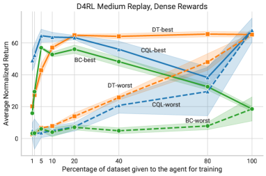
(a)

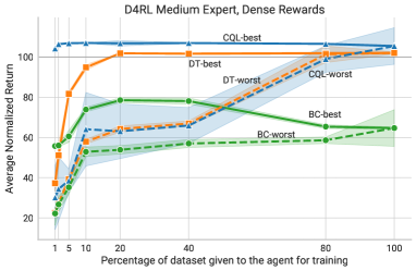
(b)

Figure 1: Normalized d4rl returns obtained by training DT, CQL, and BC on various amounts of highest-return (“best”) or lowest-return (“worst”) data. The left plot (a) is on medium replay data, while the right plot (b) is on medium expert data; both plots average over the halfcheetah, hopper and walker tasks. Notice that the Y-axis limits are set lower on the left plot. We observe that CQL was the most sample-efficient agent when only a small amount of high-quality data was available, but it could degrade with lower-quality data. Meanwhile, the performance of DT never worsened with more data. Also, BC performed best with 20-40% of high-quality data, highlighting the importance of expert data for BC. For full results, refer to Figure 8 in Appendix E.

4.3 How are agents affected when trajectory lengths in the dataset increase?

In this section, we study how performance varies as a function of trajectory lengths in the dataset; this is an important question because, in practice, data suboptimality often manifests as longer demonstrations. To study this question, we turned to human demonstrations, which are qualitatively different from synthetic data Orsini et al. (2021): human behavior is multi-modal and may be non-Markovian, so humans exhibit greater diversity in demonstration lengths when solving a task. We used the robomimic benchmark, which contains PH (proficient human) and MH (multi-human) sparse-reward datasets (Section 3.2). Because the rewards are fixed and given at the end of trajectories, the lengths of the trajectories are a proxy for optimality, as highlighted by Mandlekar et al. (2021). The MH datasets are further broken into “Better,” “Okay,” and “Worse” splits based on the proficiency of the demonstrator. We leveraged this to do more granular experimentation. See Table 4 for results.

Dataset Type	Training Trajectory Length	DT	CQL	BC
PH	$105\pm 13$	83.1 $\pm$ 0.8	45.6 $\pm$ 5.0	91.3 $\pm$ 0.9
MH-Better	$133\pm 33$	$53.5\pm 0.6$	$36.5\pm 4.7$	80.2 $\pm$ 2.3
MH-Better-Okay	$156\pm 50$	$65.3\pm 1$	$39.3\pm 5.0$	82.2 $\pm$ 2.3
MH-Okay	$180\pm 51$	$54.2\pm 0$	$29.8\pm 4.9$	65.1 $\pm$ 2.6
MH-Better-Okay-Worse	$194\pm 93$	$72.2\pm 1.2$	$26.5\pm 4.4$	79.6 $\pm$ 3.6
MH-Better-Worse	$201\pm 107$	$60.0\pm 0.8$	$32.4\pm 10.7$	74.2 $\pm$ 3.3
MH-Okay-Worse	$224\pm 99$	$52.9\pm 0.5$	$28.7\pm 2.3$	67.4 $\pm$ 3.4
MH-Worse	$269\pm 113$	$52.4\pm 0$	$5.8\pm 4.1$	59.5 $\pm$ 6.8

Table 4: Average training trajectory length and corresponding success rates for DT, CQL, and BC on human-generated datasets in robomimic. Each row aggregates over the Lift, Can, and Square tasks.

We see that BC outperformed all other agents. All methods performed best using shortest trajectories and deteriorated similarly as trained on longer trajectories. For full results, refer to Table 11 in Appendix E. The finding that BC performed best is especially interesting in light of Table 3, where BC performed far worse than DT. The difference is that Table 3 was on MG (machine-generated) data, while Table 4 studies human-generated data. Orsini et al. (2021) have found the source of data to play a prominent role in determining how well an agent performs on a task. This finding is consistent with many prior works Brandfonbrener et al. (2022); Mandlekar et al. (2021); Bahl et al. (2022); Gandhi et al. (2022); Wang et al. (2023); Lu et al. (2022) that have found Imitation Learning to work better than Q-Learning when the policy is trained on human-generated data.

As trajectory lengths increase, bootstrapping methods are susceptible to worse performance because values must be propagated over longer time horizons. This is especially a challenge in sparse-reward settings and may explain why we observed CQL performing far worse than BC and DT.

Given that we used a context length of 1 for DT in robomimic (Section 3.2), the key differences between BC and DT are 1) conditioning on returns-to-go, and 2) the MLP versus Transformer architecture. We hypothesize that BC performs better than DT because the PH and MH datasets are high-quality enough for Imitation Learning to be effective while being too small for Sequence Modeling. Refer to Appendix D for a detailed study that attempts to disentangle these differences.

4.4 How are agents affected when random data is added to the dataset?

This section explores the impact of adding an equal amount of data collected from a random policy to our training dataset. We considered two strategies to ensure our results were not skewed based on a particular strategy for collecting random data. In “Strategy 1,” we rolled out a uniformly random policy from sampled initial states. In “Strategy 2,” we rolled out a pre-trained DT agent for several steps and executed a single uniformly random action. The number of steps in each rollout was chosen uniformly at random to be within 1 standard deviation of the average trajectory length in the offline dataset. We can see that Strategy 1 adds random transitions around initial states, while Strategy 2 adds random transitions along the entire trajectory leading to goal states. Because results did not differ significantly between the two strategies (see Appendix E.4), Figure 2 shows results averaged across both. Akin to Section 4.1, we consider dense- and sparse-reward settings in d4rl and robomimic.

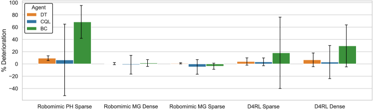
Figure 2: The impact of adding random data to the offline dataset for DT, CQL, and BC. The Y-axis shows the relative deterioration in the evaluation score. Results are averaged over tasks and over two strategies for creating random data. The robomimic PH dataset does not have a dense-reward split.

Compared to BC, both CQL, and DT demonstrated enhanced robustness to injected data, experiencing less than 10% deterioration. However, the resilience of these agents manifests differently. CQL’s resilience is more volatile than DT’s, as evidenced by the larger standard deviations of blue bars compared to orange ones. In Appendix E.4, we present a per-task breakdown of the results in Figure 2, which shows several intriguing trends. CQL’s performance varies greatly across tasks: it improves in some, remains stable in others, and deteriorates in the rest. Interestingly, when CQL’s performance on the original dataset is poor, adding random data can occasionally improve it, as corroborated by Figure 1. CQL’s volatility is particularly apparent in robomimic, with Figure 14 showing that CQL deteriorates nearly 100% on the Lift PH dataset but improves on the Can PH dataset by nearly 2x.

The low deterioration of BC on robomimic MG is likely just because the MG data was generated from several checkpoints of training a SAC agent, and therefore already has significantly lower data quality than either robomimic PH or d4rl. In Section 4.3, we found Imitation Learning to be superior when the behavior policy was driven by humans. However, when suboptimal data is mixed with high-quality human data, Sequence Modeling becomes preferable over Imitation Learning.

4.5 How are agents affected by the complexity of the task?

We now focus on understanding how increasing the task complexity impacts the performance of our agents. Two major factors contributing to task complexity are the dimensionality of the state space and the horizon of the task MDP. To understand the impact of state space dimensionality, we utilized the humanoid environment, which has $376$-dimensional states, along with other d4rl tasks, which have substantially smaller state spaces. To understand the impact of task horizon, we utilized the robomimic PH datasets for Lift, Can, Square, and Transport tasks (listed in order of increasing task horizon). Although trajectory lengths in the dataset are an artifact of the behavior policy while task horizon is an inherent property of the task, we found average trajectory lengths in the dataset to be a useful proxy for quantifying task horizon, because exactly computing task horizon is non-trivial. Akin to the previous section, we experimented with both the PH datasets and the same datasets with an equal amount of random data added in. Figure 3 shows the results averaged on tasks with identical dimensions (left) and task horizon (right) for DT, CQL, and BC.

The performance of all agents degraded roughly equally as the state space dimensionality increased ($11\rightarrow 17\rightarrow 376$). Regarding task horizon, with high-quality data (PH), all three agents started near a 100% success rate, but BC deteriorated least quickly, followed by DT and then CQL. In the presence of the suboptimal random data (PH-suboptimal), DT performed the best while BC performed poorly, consistent with our observations in Section 4.4. Additionally, CQL benefited from the addition of suboptimal data, as seen by comparing the solid and dotted blue lines. This suggests that adding such data can improve the performance of CQL in long-horizon tasks, consistent with Figure 1.

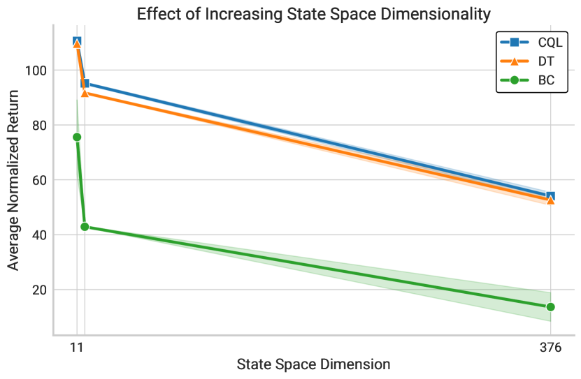
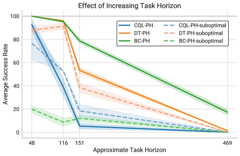
Figure 3: Impact of increasing state-space dimensionality on d4rl medium expert data (left) and task horizon on robomimic with both PH data and PH + equal amount of random data (right).

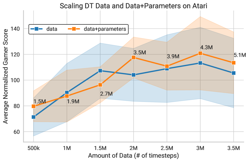
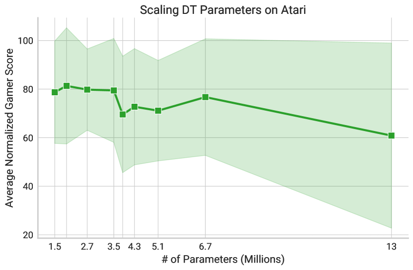
Figure 4: atari results for DT while scaling data only (left, blue), parameters only (right), and both simultaneously (left, orange), averaged over breakout, qbert, seaquest, and pong. Numbers on top of the orange curve show model parameter sizes. We found that scaling data was more impactful than scaling parameters, but scaling both together gave minor gains over scaling data only.

4.6 Scaling Properties of Decision Transformers on Atari

Based on the relative robustness of Sequence Modeling in the previous sections, we studied the scaling properties of DT along three dimensions: the amount of training data, the number of model parameters, and both jointly. We focused on the atari benchmark because of its high-dimensional observations, for which we expect scaling to be most helpful. We scaled the number of model parameters by increasing the number of layers in the DT architecture $\in\{6,8,12,16,18,20,24,32,64\}$.

The results are shown in Figure 4. The performance of DT reliably increased with more data up until 1.5M timesteps in the dataset (blue, left), but was insensitive to or perhaps even hurt by increasing the number of parameters (green, right). Upon scaling DT to a certain size (3.5M+ parameters), we observed that the larger model outperformed its smaller counterpart given the same amount of data.

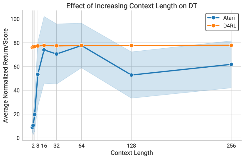
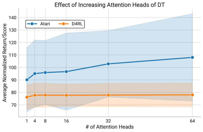
Figure 5: Increasing the context length (left) and number of attention heads (right) of DT on both atari and d4rl. atari curves average over breakout, qbert, seaquest, and pong. d4rl curves average over all tasks and data splits. We see that scaling context length and attention heads benefits performance on atari, but not on d4rl, though the observed benefit of increasing the number of attention heads is not statistically significant.

4.7 Architectural Properties of Decision Transformers

Finally, we study the impact of architectural properties of DT, namely the context length, # of attention heads, # of layers, and embedding size. Full experimental results are in Appendix G.

Context length: The use of a context window makes DT dependent on the history of states, actions, and rewards, unlike CQL and BC. Figure 5 (left) demonstrates the role of context length for DT. Having a context length larger than 1 (i.e., no history) did not benefit DT on d4rl, while it helped on atari, where performance is maximized at a context length of 64. This finding indicates that some tasks may benefit from a more extensive knowledge of history than others. The deterioration in performance, as context length increases, is likely due to DT overfitting to certain trajectories.

Attention Heads: While the importance of the number of Transformer attention heads has been noted in NLP Michel et al. (2019), it is an open question how the trends carry over to offline RL. Figure 5 (right) shows the impact of this hyperparameter on DT. We observed monotonic improvement on atari, but no improvement on d4rl. One of the primary reasons for this discrepancy is that there is more room for an agent to extract higher rewards on atari than d4rl. For instance, DT achieved an expert-normalized score of over $320$ on the breakout atari game, but never gets over $120$ in d4rl. This suggests there is more room for scaling the architecture to improve results on atari.

Number of layers: This was discussed in Section 4.6, with results in Figure 4.

Embedding size: Increasing the embedding size of DT beyond 256 did not result in any improvement in atari; see Table 20 in Appendix G for results.

5 Limitations and Future Work

This work addressed the question of which learning paradigm should be preferred for offline reinforcement learning, among Q-Learning, Imitation Learning, and Sequence Modeling. We highlighted several practical takeaways throughout the paper, and summarized our findings in Table 1.

There are several limitations of our work, which serve as avenues for future research. First, our findings are based off deterministic benchmarks; it would be interesting to study the sensitivity of offline RL algorithms to the amount of stochasticity in the environment Paster et al. (2022). Additionally, we could broaden our study to include more representative algorithms from each paradigm, such as Implicit Q-Learning Kostrikov et al. (2021) and Trajectory Transformers Janner et al. (2021), as well as paradigms we did not explore here, such as model-based offline RL Kidambi et al. (2020b); Yu et al. (2020b). Finally, we hope to evaluate on a larger set of benchmarks that includes more compositional tasks, like those in the embodied AI literature Duan et al. (2022).

Appendix A Extended Background

In the reinforcement learning (RL) problem, an agent interacts with a Markov decision process (MDP) Puterman (1990), defined as a tuple $(\mathcal{S},\mathcal{A},T,R,H)$, where $\mathcal{S}$ and $\mathcal{A}$ denote the state and action spaces, $T(s^{\prime},a,s)=\Pr(s^{\prime}|s,a)$ is the transition model, $R(s,a)\in\mathbb{R}$ is the reward function, and $H$ is the (finite) horizon. At each timestep, the agent takes an action $a\in\mathcal{A}$, the environment state transitions according to $T$, and the agent receives a reward according to $R$. The agent does not know $T$ or $R$. Its objective is to obtain a policy $\pi:\mathcal{S}\to\mathcal{A}$ such that acting under the policy maximizes its return, the sum of expected rewards: $\mathbb{E}[\sum_{t=0}^{H}R(s_{t},\pi(s_{t}))]$. In offline RL Levine et al. (2020), agents cannot interact with the MDP but instead learn from a fixed dataset of transitions $\mathcal{D}=\{(s,a,r,s^{\prime})\}$, generated from an unknown behavior policy.

Q-Learning and CQL. One of the most widely studied learning paradigms is Q-Learning Sutton and Barto (2018), which uses temporal difference (TD) updates to estimate the value of taking actions from states via bootstrapping. Although Q-Learning promises to provide a general-purpose decision-making framework, in the offline setting algorithms such as Conservative Q-Learning (CQL) Kumar et al. (2020) and Implicit Q-Learning (IQL) Kostrikov et al. (2021) are often unstable and highly sensitive to the choice of hyperparameters Brandfonbrener et al. (2022). In this paper, we will focus on Conservative Q-Learning (CQL). CQL Kumar et al. (2020) proposes a modification to the standard Q-learning algorithm to address the overestimation problem by constraining the Q-values so that they do not exceed a lower bound. This constraint is highly effective in the offline setting because it mitigates the distributional shift between the behavior policy and the learned policy. More concretely, CQL adds a regularization term to the standard Bellman update:

$$\min_{\theta}~{}\alpha\!\left(\mathbb{E}_{s\sim\mathcal{D}}\left[\log\left(\sum_{a^{\prime}}\exp(Q_{\theta}(s,a^{\prime}))\right)\right]\!-\!\mathbb{E}_{s,a\sim\mathcal{D}}\left[Q_{\theta}(s,a)\right]\right)+\mathsf{TDError}(\theta;\mathcal{D}),$$ (1)

where $\alpha$ is the weight given to the first term, and the second term is the distributional $\mathsf{TDError}(\theta;\mathcal{D})$ under the dataset, from C51 Bellemare et al. (2017).

Imitation Learning and BC. When the dataset comes from expert demonstrations or is otherwise near-optimal, researchers often turn to imitation learning algorithms such as Behavior Cloning (BC) or TD3+BC Fujimoto and Gu (2021b) to train a policy. BC is a simple imitation learning algorithm that performs supervised learning to map states $s$ in the dataset to their associated actions $a$. Due to the reward-agnostic nature of BC, it typically requires expert demonstrations to learn an effective policy. The clear downside of BC is that the imitator cannot be expected to attain higher performance than was attained in the dataset.

Sequence Modeling and DT. Sequence modeling is a recently popularized class of offline RL algorithms that includes the Decision Transformer Chen et al. (2021) and the Trajectory Transformer Janner et al. (2021). These algorithms train autoregressive sequence models that map the history of the trajectory to the next action. In the Decision Transformer (DT) model, the learned policy produces action distributions conditioned on trajectory history and desired returns-to-go $\hat{R}_{t^{\prime}}=\sum_{t=t^{\prime}}^{T}r_{t}$. This leads to the following trajectory representation, used for both training and inference: $\tau=(\hat{R}_{1},s_{1},a_{1},\hat{R}_{2},s_{2},a_{2},\ldots,\hat{R}_{T},s_{T},a_{T})$. Conditioning on returns-to-go enables DT to learn effective policies from suboptimal data and produce a range of behaviors during inference.

Appendix B Additional Dataset Details

Humanoid Data

In this section, we present the details of the humanoid offline Reinforcement Learning (RL) dataset created for our experiments. We trained a Soft Actor-Critic (SAC) agent Haarnoja et al. (2018) for 3 million steps and selected the best-performing agent, which achieved a score of 5.5k, to generate the expert split. To create the medium split, we utilized an agent that performed at one-third of the expert’s performance. We then generated the medium-expert split by concatenating the medium and expert splits. Our implementation is based on (Raffin et al., 2021) and employs the default hyperparameters for the SAC agent (behavior policy). Table 5 displays the performance of all agents across all splits of the humanoid task. Furthermore, Table 6 provides statistical information on the humanoid dataset.

Task	BC	DT	CQL
Humanoid Medium	13.22 $\pm$ 4.25	23.67 $\pm$ 2.48	49.51 $\pm$ 0.77
Humanoid Medium Expert	13.67 $\pm$ 5.21	52.63 $\pm$ 1.92	54.1 $\pm$ 1.36
Humanoid Expert	24.22 $\pm$ 5.37	53.41 $\pm$ 1.32	63.69 $\pm$ 0.22
Average	17.03	43.23	55.76

Table 5: Performance of agents on a high dimensional state space task. CQL seems better suited to tasks involving higher state space dimensions.

Task	# of trajectories	# of samples
Humanoid Medium	4000	1.76M
Humanoid Expert	4000	3.72M
Humanoid Medium Expert	8000	5.48M

Table 6: Dataset statistics for humanoid. The number of samples refers to the number of environment transitions recorded in the dataset.

Robomimic:

We visualize the return distribution of robomimic tasks, employing a discount factor of 0.99, as illustrated in Figure 6 and Figure 7. It becomes evident that the discount factor has a significant impact on the data’s optimality characteristics. PH features shorter trajectories, resulting in a higher proportion of high-return data.

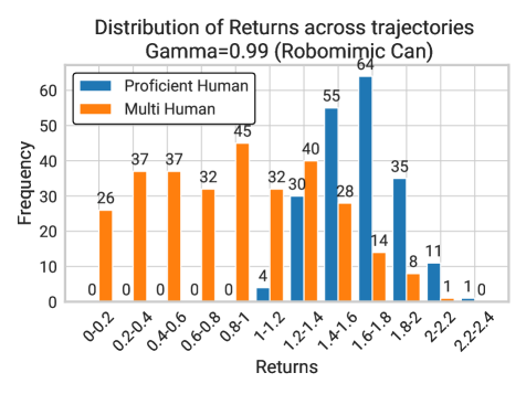
Figure 6: Reward Distribution in Proficient and Multi Human splits of Robomimic Can environment shown with gamma set to 0.99. Proficient Human trajectories are shorter in length compared to Multi Human trajectories. Even though PH and MH datasets contain the same number of trajectories, the PH dataset contains more near-expert data.

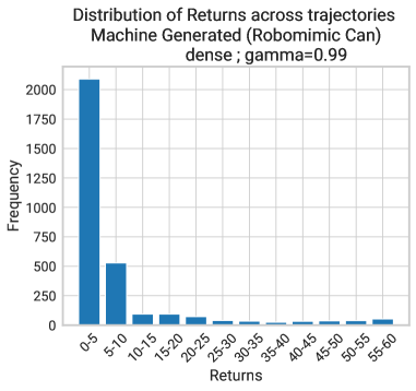
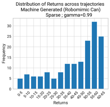
Figure 7: Reward Distribution in Machine Generated splits of Robomimic Can environment is shown with gamma set to 0.99. The sparse variant has more high return trajectories.

Appendix C Additional Evaluation Details

We specify our sampling procedure used to evaluate the atari benchmark, used in Section 4.6 and Section 4.7. The atari offline dataset Agarwal et al. (2020) contains the interaction of a DQN agent Mnih et al. (2015) as it is trained progressively in 50 buffers. Each observation in the dataset contains the last 4 frames of the game, stacked together. Buffers 1 and 50 would contain interactions of the DQN agent when it is naive and expert respectively. Our results are averaged across four different experiments. Each experiment performed a sampling of 500k timestep data from the buffers numbered 1) 1-50 2) 40-50 (DQN is competitive), 3) 45-50, and 4) 49-50 (DQN is expert). We study the architectural and scaling properties of DT in this dataset, where we consider four games: breakout, qbert, seaquest, and pong. We follow the protocol of Lee et al. (2022) and Kumar et al. (2023) by training on the Atari DQN Replay dataset, which used sticky actions, but then evaluating with sticky actions disabled.

Appendix D Disentangling DT and BC

In this section, we experimented with an additional baseline, “BC Transformer,” a modified version of DT that does not perform conditioning on a returns-to-go vector and has a context length of 1. As previously mentioned, we set the context length to 1 in the case of DT for running experiments on robomimic as well. This section aims to investigate the discrepancy between the performance of DT and BC, specifically, we wanted to understand how much of the discrepancy can be attributed to RTG conditioning compared to architectural differences between DT and BC which is typically implemented using a stack of MLPs. By having the BC Transformer baseline, the only distinguishing component between it and BC is the architecture. We observed that BC is often a better-performing agent than BC Transformer on PH Table 7, MG Table 8, and MH tasks Table 9. Additionally, it can also be observed that RTG conditioning only plays a critical role when the distribution of reward shows variation. Unlike expert data such as PH and MH where the RTG vector remained the same, we see DT outperforming BC Transformer on MG significantly.

Layers	BC Transformer	DT	BC	CQL
Lift-PH	$100\pm 0$	$100\pm 0$	$100\pm 0$	$92.7\pm 5$
Can-PH	$94.6\pm 2.4$	$96\pm 0$	$95.3\pm 0.9$	$38\pm 7.5$
Square-PH	$52\pm 5.8$	$53.3\pm 2.4$	$78.7\pm 1.9$	$5.3\pm 2.5$
Transport-PH	$0\pm 0$	$1.3\pm 0$	$29.3\pm 0.9$	$0\pm 0$

Table 7: Results of agents on robomimic PH tasks

Layers	BC Transformer	DT	BC	CQL
Lift-MG-sparse	$77.9\pm 7.11$	$96\pm 2.1$	$65.3\pm 2.5$	$64\pm 2.8$
Can-MG-sparse	$48.66\pm 1.8$	$92.8\pm 4.1$	$64.7\pm 3.4$	$1.3\pm 0.9$
Lift-MG-dense	$68\pm 3.2$	$93.99\pm 2.5$	$60\pm 2$	$63.3\pm 5.2$
Can-MG-dense	$43.99\pm 3.2$	$82.4\pm 4.2$	$64\pm 4.3$	$0\pm 0$

Table 8: Results of agents on robomimic MG tasks

Layers	BC Transformer	DT	BC	CQL
Lift-MH	$100\pm 0$	$100\pm 0$	$100\pm 0$	$56.7\pm 40.3$
Can-MH	$93.3\pm 4.1$	$95.33\pm 0$	$86\pm 4.3$	$22\pm 5.7$
Square-MH	$18.66\pm 4.1$	$21.33\pm 3.7$	$52.7\pm 6.6$	$0.7\pm 0.9$
Transport-MH	$0\pm 0$	$0\pm 0$	$11.3\pm 2.5$	$0\pm 0$

Table 9: Results of agents on robomimic MH tasks

Appendix E Additional Results on d4rl and robomimic

This section contains results obtained on individual tasks of d4rl and robomimic benchmarks. We use the averaged-out results obtained on all of the tasks from the respective benchmark for our analysis.

E.1 Establishing baselines

This section presents baseline results for individual tasks in both sparse and dense settings of the D4RL. The average outcomes are detailed in Table 2 (Section subsection 4.1). Our observations indicate that DT consistently outperforms CQL and BC in nearly all tasks within the sparse setting of the D4RL benchmark. Although CQL achieves a marginally higher average return on the Hopper task (3.4% ahead of DT for medium and medium-replay splits), it also exhibits significantly higher volatility, as evidenced by the standard deviations. In contrast, DT remains competitive and robust. In the sparse reward setting, CQL surpasses BC by 5.2%. As highlighted in Section subsection 4.1, CQL is most effective in the dense reward setting of the D4RL benchmark.

Dataset	DT		CQL		BC
	Sparse	Dense	Sparse	Dense
Medium
Half Cheetah	42.54 $\pm$ 0.12	$42.55\pm 0.02$	$38.63\pm 0.81$	$47.03\pm 0.075$	$42.76\pm 0.17$
Hopper	$69.75\pm 2.31$	$73.03\pm 0.74$	73.89 $\pm$ 10.12	$70.54\pm 0.41$	$64.35\pm 5.6$
Walker	75.42 $\pm$ 1.07	$75.42\pm 0.9$	$19.31\pm 3.17$	$83.77\pm 0.25$	$54.62\pm 12.04$
Average	62.56 $\pm$ 1.16	63.66 $\pm$ 0.55	43.94 $\pm$ 4.7	67.11 $\pm$ 0.24	53.91 $\pm$ 5.93
Medium Replay
Half Cheetah	38.76 $\pm$ 0.26	$37.09\pm 0.4$	$35\pm 2.56$	$46.12\pm 0.06$	$9.81\pm 9.2$
Hopper	$82.24\pm 1.58$	$89.15\pm 1.19$	83.1 $\pm$ 19.21	$101.27\pm 0.46$	$16.19\pm 10.8$
Walker	71.24 $\pm$ 1.93	$69.44\pm 3.14$	$29.02\pm 19.63$	$87.85\pm 0.83$	$17.82\pm 4.96$
Average	64.08 $\pm$ 1.25	65.22 $\pm$ 1.57	49.04 $\pm$ 13.79	78.41 $\pm$ 0.45	14.6 $\pm$ 8.32
Medium Expert
Half Cheetah	90.55 $\pm$ 1.53	$91.67\pm 0.21$	$24.35\pm 2.38$	$94.95\pm 0.25$	$42.95\pm 0.14$
Hopper	110.29 $\pm$ 0.58	$110.76\pm 0.06$	$42.44\pm 12.52$	$109.67\pm 2.12$	$62.21\pm 6.5$
Walker	108.63 $\pm$ 0.22	$108.49\pm 0.1$	$21.3\pm 0.55$	$111.58\pm 0.17$	$38\pm 9.86$
Average	103.15 $\pm$ 0.77	103.64 $\pm$ 0.12	29.36 $\pm$ 5.14	105.39 $\pm$ 0.84	47.72 $\pm$ 5.5
Total Average	76.6 $\pm$ 1	77.51 $\pm$ 1.12	40.78 $\pm$ 7.88	83.64 $\pm\textbf{0.51}$	38.74 $\pm$ 6.58

Table 10: Results on d4rl in both sparse and dense reward settings, averaged over the halfcheetah, hopper, and walker tasks. The presented results here are an extension of Table 2.

E.2 How does the amount and quality of data affect each agent’s performance?

Figure 8 illustrates the performance of agents on individual tasks within the D4RL benchmark as data quality and quantity are varied. DT improved or plateaued (upon reaching maximum performance) as additional data was provided. In contrast, CQL exhibits volatility, displaying significant performance declines in hopper and walker2d medium-replay tasks. The performance of BC tends to deteriorate when trained on low-return data.

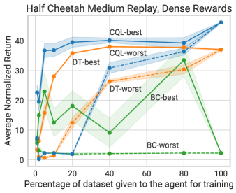
(a)

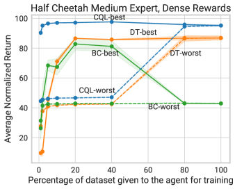
(b)

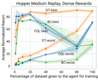
(c)

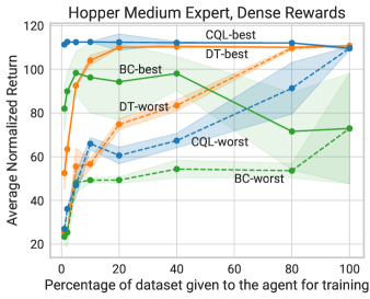
(d)

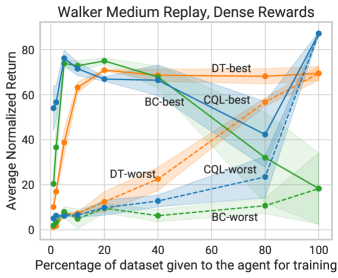
(e)

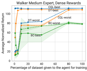
(f)

Figure 8: Results demonstrating the behavior of agents as the amount of data and quality is varied on medium-replay and medium-expert splits of d4rl benchmark in dense reward setting. The results presented here are an extension of Figure 1.

Figure 9 illustrates the performance behavior of agents as the quantity and quality of data are adjusted in a sparse setting on the d4rl dataset. A more detailed exploration of this behavior across individual tasks is presented in Figure Figure 10.

Two key observations can be made from these results. 1) In the sparse reward setting, DT becomes a markedly more sample-efficient choice, with its performance either improving or remaining steady as the quantity of data increases. In contrast, CQL displays greater variability and fails to exceed BC in scenarios involving expert data (medium-expert). 2) The sub-optimal data plays a significantly more important role for CQL in sparse settings as compared to dense settings. Our hypothesis is that the sparsity of feedback makes learning about course correction more critical than learning from expert demonstrations. Notably, we discovered that the worst 10% of data features trajectories with substantially higher return coverage, which contributes to greater diversity within the data. This, in turn, enhances CQL’s ability to learn superior Q-values (course correction) when compared to the best 10% of data in a medium-expert data setting.

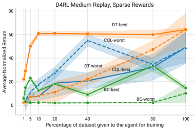
(a)

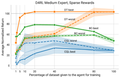
(b)

Figure 9: Normalized d4rl returns obtained by training DT, CQL, and BC on various amounts of highest-return (“best”) or lowest-return (“worst”) data in sparse reward setting. The left plot (a) is on medium replay data, while the right plot (b) is on medium expert data; both plots average over the halfcheetah, hopper and walker tasks. Notice that the Y-axis limits are set lower on the left plot. We observed that DT was a substantially more sample-efficient agent than CQL. Sub-optimal data was noticeably crucial for CQL in sparse reward setting.

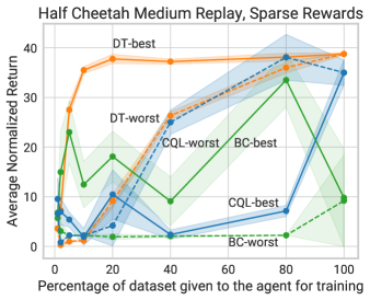
(a)

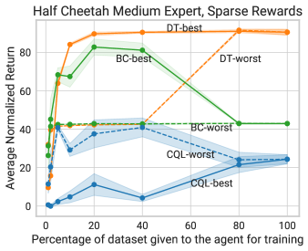
(b)

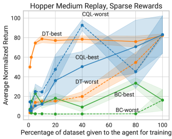
(c)

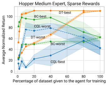
(d)

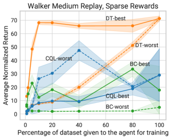
(e)

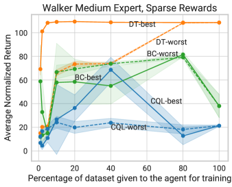
(f)

Figure 10: Results demonstrating the behavior of agents as the amount of data and quality is varied on medium-replay and medium-expert splits of d4rl benchmark in sparse reward setting.

E.3 How are agents affected when trajectory lengths in the dataset increase?

Table 11 showcases the performance of all agents across individual robomimic tasks, encompassing both synthetic and human-generated datasets. DT surpasses both agents in all synthetic tasks within the robomimic benchmark, for both sparse and dense settings. Interestingly, BC demonstrates a strong aptitude for numerous tasks with human-generated data, particularly excelling on the square task.

Dataset Type	Average Trajectory Length	DT	CQL	BC
Lift MG Dense	150 $\pm$ 0	96 $\pm$ 1.2	$68.4\pm 6.2$	59.2$\pm 6.19$
Lift MG Sparse	150 $\pm$ 0	93.2 $\pm$ 3.2	60$\pm$13.2	59.2$\pm 6.19$
Can MG Dense	150 $\pm$ 0	83.2 $\pm$ 0	$2\pm 1.2$	49.6$\pm$2.4
Can MG Sparse	150 $\pm$ 0	83.2 $\pm$ 1.59	$0\pm 0$	49.6$\pm$2.4
Lift-PH	48 $\pm$ 6	100 $\pm$ 0	$92.7\pm 5$	100$\pm 0$
Lift-MH-Better	72 $\pm$ 24	94.6 $\pm$ 1.8	$88\pm 5.9$	98.7 $\pm$ 1.9
Lift-MH-Okay-Better	83 $\pm$ 29	100 $\pm$ 0	$86\pm 6.5$	99.3 $\pm$ 0.9
Lift-MH-Okay	94 $\pm$ 30	97.33 $\pm$ 0	$67.3\pm 10.5$	96 $\pm$ 1.6
Lift-MH	104 $\pm$ 44	100 $\pm$ 0	$56.7\pm 5$	100 $\pm$ 0
Lift-MH-Worse-Better	109 $\pm$ 49	100 $\pm$ 0	$75.3\pm 25.6$	100 $\pm$ 0
Can-PH	116 $\pm$ 14	96 $\pm$ 0	$38.7\pm 7.5$	95.3$\pm 0.9$
Lift-MH-Worse-Okay	119 $\pm$ 44	100 $\pm$ 0	$64.7\pm 2.5$	98.7 $\pm$ 1.9
Can-MH-Better	143 $\pm$ 29	$52.66\pm 0$	$20.7\pm 7.4$	83.3 $\pm$ 2.5
Lift-MH-Worse	145 $\pm$ 40	$94.6\pm 0$	$13.3\pm 9$	100 $\pm$ 0
Square-PH	151 $\pm$ 20	53.3 $\pm$ 2.4	5.3 $\pm$ 2.5	78.7 $\pm$ 1.9
Can-MH-Okay-Better	162 $\pm$ 44	$75.33\pm 3.3$	$30.7\pm 7.7$	90.7 $\pm$ 1.9
Can-MH-Okay	181 $\pm$ 47	$52.66\pm 0$	$22\pm 4.3$	72 $\pm$ 2.8
Square-MH-Better	185 $\pm$ 46	13.3 $\pm$ 0	0.7 $\pm$ 0.9	58.7 $\pm$ 2.5
Can-MH	209 $\pm$ 114	95.33 $\pm$ 0	$22\pm 7.5$	$86\pm 4.3$
Can-MH-Worse-Better	224 $\pm$ 134	73.99 $\pm$ 1.1	$20.7\pm 5.7$	76 $\pm$ 4.3
Square-MH-Okay-Better	225 $\pm$ 76	20.66 $\pm$ 0	1.3 $\pm$ 0.9	56.7 $\pm$ 4.1
Can-MH-Worse-Okay	242 $\pm$ 126	$54\pm 1.6$	$18.8\pm 2.5$	74.7 $\pm$ 5.7
Square-MH-Okay	265 $\pm$ 78	12.6 $\pm$ 0	0 $\pm$ 0	27.3 $\pm$ 3.4
Square-MH	269 $\pm$ 123	21.33 $\pm$ 3.7	0.7 $\pm$ 0.9	52.7 $\pm$ 6.6
Square-MH-Worse-Better	271 $\pm$ 140	6 $\pm$ 0	1.3 $\pm$ 0.9	46.7 $\pm$ 5.7
Can-MH-Worse	304 $\pm$ 148	$51.33\pm 0$	$4\pm 3.3$	56.7 $\pm$ 2.5
Square-MH-Worse-Okay	311 $\pm$ 128	4.6 $\pm$ 0	2.7 $\pm$ 1.9	28.7 $\pm$ 2.5
Square-MH-Worse	357 $\pm$ 150	11.3 $\pm$ 0	0 $\pm$ 0	22 $\pm$ 4.3

Table 11: Success rates for different synthetic and human-generated datasets in robomimic. Results presented here are an extension of Table 4 (from subsection 4.3) and have been sorted as per the trajectory length of the task. DT outperformed both agents on synthetic data as seen by performance on MG tasks. BC seemed well suited to numerous tasks for which data was human-generated (PH and MH). Bold numbers represent the best-performing agent on the corresponding task.

E.4 How are agents affected when suboptimal data is added to the dataset?

Figure 11 depicts the behavior of agents when random data is introduced according to “Strategy 1” in the dense reward data regime of the D4RL benchmark. As previously described, “Strategy 1” involves rolling out a uniformly random policy from sampled initial states to generate random data. Our observations indicate that both CQL and DT maintain stable performance, while BC exhibits instabilities, occasionally failing as observed in the half cheetah task.

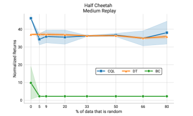
(a)

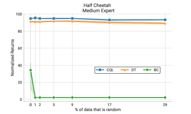
(b)

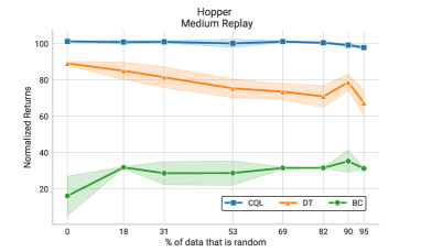
(c)

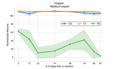
(d)

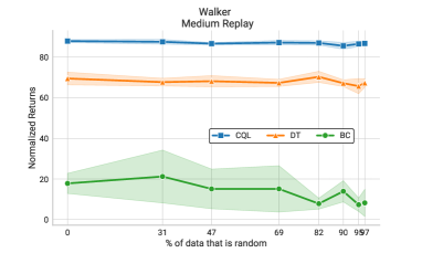
(e)

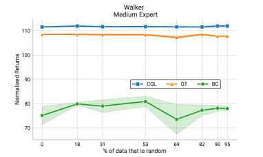
(f)

Figure 11: Impact of adding suboptimal data on all agents in dense reward data regime on D4RL tasks using Strategy 1. The results presented here are an extension to Figure 2 (from subsection 4.4).

Figure 12 displays the behavior of agents as random data is incorporated according to Strategy 2 in the dense reward data regime of the D4RL benchmark. In "Strategy 2," we roll out a pre-trained agent for a certain number of steps, execute a single uniformly random action, and then repeat the process. While Strategy 1 produces random transitions primarily clustered around initial states, Strategy 2 generates random transitions across the entire manifold of states, spanning from initial states to high-reward goal states.

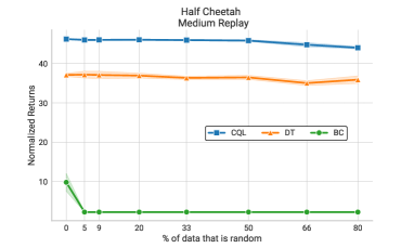
(a)

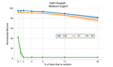
(b)

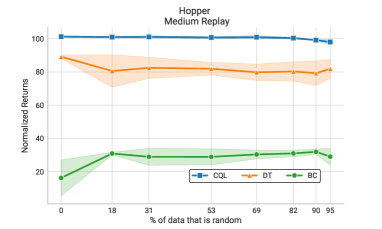
(c)

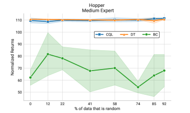
(d)

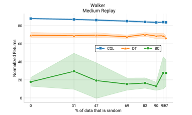
(e)

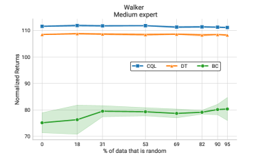
(f)

Figure 12: Impact of adding suboptimal data in dense reward data regime on D4RL tasks using Strategy 2. The results presented here are an extension to Figure 2 (from subsection 4.4). A noteworthy observation from this experiment is that the performance of CQL improved on hopper medium-expert task with the addition of random data. This suggests that the random data might be aiding in the learning of more accurate Q-values for various states.

Figure 13 illustrates the behavior of agents when random data is introduced according to Strategy 2 in the sparse reward data regime of the d4rl benchmark. We observed that the performance of CQL drastically declined on the hopper-medium-replay task, while its performance stayed the same on other tasks.

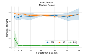
(a)

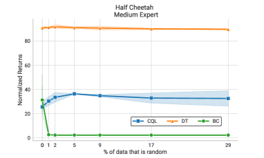
(b)

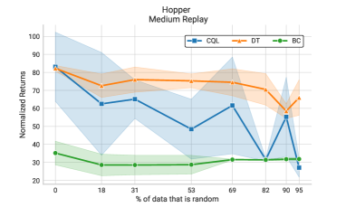
(c)

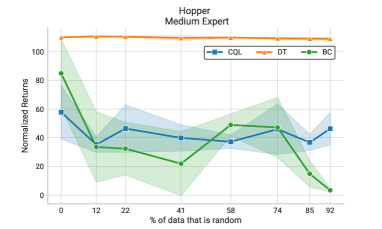
(d)

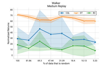
(e)

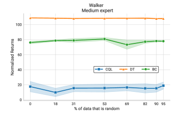
(f)

Figure 13: Impact of adding suboptimal data in sparse reward data regime on d4rl tasks using Strategy 2. The results presented here are an extension to Figure 2 (from subsection 4.4). The performance of CQL sharply decreases in the hopper medium-replay task. Unlike its performance in the dense reward data regime, CQL does not exhibit the same level of resilience in the sparse reward setting and demonstrates considerably higher volatility.

Figure 14 depicts the behavior of agents when random data is incorporated following Strategy 1 in the sparse reward data regime (human-generated) of the robomimic benchmark. Notably, we observed drastically different performance trends with CQL. Its performance plummeted by 80% when the proportion of random data reached 51%. In contrast, its performance nearly doubled on the can mg task when the proportion of random data was increased to 30%.

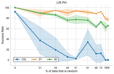
(a)

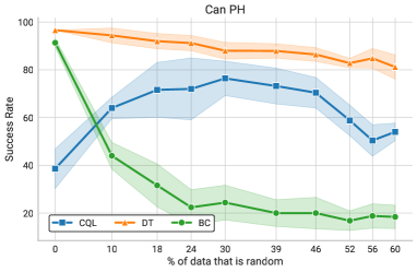
(b)

Figure 14: Impact of adding suboptimal data in sparse reward data regime in robomimic using Strategy 1. The results presented here are an extension to Figure 2 (from subsection 4.4). CQL exhibited markedly different behaviors across these tasks. Its performance declined sharply on the lift ph task. In contrast, its performance significantly improved, nearly doubling, with the addition of random data on can ph task.

Figure 15 illustrates the behavior of agents when random data is introduced according to Strategy 2 in the sparse reward data regime (human-generated) of the robomimic benchmark.

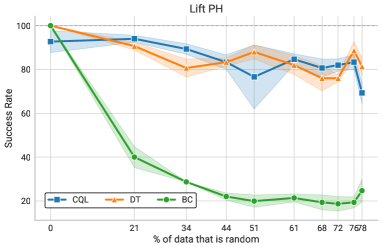
(a)

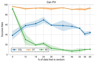
(b)

Figure 15: Impact of adding suboptimal data in sparse reward data regime in robomimic using Strategy 2. The results presented here are an extension to Figure 2 (from subsection 4.4). Interestingly, when following Strategy 2 for random data generation, CQL maintains stable performance in the lift ph task. We observed a similar behavior to that seen with Strategy 1 on the can ph task.

Figure 16 and Figure 17 presents the behavior of agents as random data is added following Strategy 2 in sparse and dense reward data regime (synthetic) respectively on the robomimic benchmark. In all four scenarios, DT maintained its peak performance reasonably well, indicating its resilience in very noisy data settings. Conservative Q-Learning (CQL), however, showed signs of deterioration on both dense and sparse variants of Lift tasks. Notably, CQL failed to perform on the can task. As mentioned earlier, BC didn’t exhibit deterioration, possibly because the Mixed-Goal (MG) data already contains a substantial amount of highly sub-optimal data.

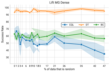
(a)

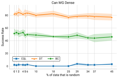
(b)

Figure 16: Impact of adding suboptimal data in dense reward data regime in robomimic using Strategy 2. The results presented here are an extension to Figure 2 (from subsection 4.4).

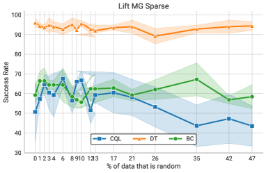
(a)

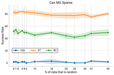
(b)

Figure 17: Impact of adding suboptimal data in sparse reward data regime in robomimic using Strategy 2. The results presented here are an extension to Figure 2 (from subsection 4.4.

Appendix F Additional Experimental Details

We used the original author implementation as a reference for our experiments wherever applicable. In settings where a new implementation was required, we referenced the implementation which has been known to provide competitive/state-of-the-art results on d4rl. We provide details on compute and hyperparameters below.

Compute

All experiments were run on an A100 GPU. Most experiments with DT typically require 10-15 hours of training. Experiments with CQL and BC require 5-10 hours of training. We used Pytorch 1.12 for our implementation.

Hyperparameters

We mentioned all the hyperparameters used across various algorithms below. Our implementations are based on original author-provided implementations, without any modifications to the hyperparameters. To learn more about the selection of hyperparameters, we recommend viewing the associated papers. Due to the stable training objective of DT and BC, both of these agents do not require substantial hyperparameter sweep experiments. DT was trained using Adam optimizer Kingma and Ba (2014) with a Multi-Step Learning Rate Scheduler. Each experiment was run five times to account for seed variance.

Hyperparameter	Returns-to-go
Robomimic PH	6
Robomimic MH	6
Robomimic MG	120

Table 12: Returns-to-go values used with DT on d4rl and robomimic.

Hyperparameter	Value
Reference implementation	https://github.com/kzl/decision-transformer/tree/master/atari (MIT License)
Number of attention heads	8
Number of layers	6
Embedding dimension	128
Context Length (Breakout)	30
Context Length (Qbert)	30
Context Length (Seaquest)	30
Context Length (Pong)	50
Number of buffers	50
Batch size	16
Learning Rate (LR)	$6e-4$
Number of Steps	500000
Return-to-go conditioning	$90$ Breakout ($\approx 1\times$ max in dataset)
	$2500$ Qbert ($\approx 5\times$ max in dataset)
	$20$ Pong ($\approx 1\times$ max in dataset)
	$1450$ Seaquest ($\approx 5\times$ max in dataset)
Nonlinearity	ReLU, encoder
	GeLU, otherwise
Encoder channels	$32,64,64$
Encoder filter sizes	$8\times 8,4\times 4,3\times 3$
Encoder strides	$4,2,1$
Max epochs	$5$
Dropout	$0.1$
Learning rate	$6*10^{-4}$
Adam betas	$(0.9,0.95)$
Grad norm clip	$1.0$
Weight decay	$0.1$
Learning rate decay	Linear warmup and cosine decay (see code for details)
Warmup tokens	$512*20$
Final tokens	$2*500000*K$

Table 13: Hyperparameters used with DT on atari.

Hyperparameter	Value
Reference implementation	https://github.com/kzl/decision-transformer/tree/master/gym (MIT License)
Number of layers	$3$
Number of attention heads	$1$
Embedding dimension	$128$
Nonlinearity function	ReLU
Batch size	$512$
Return-to-go conditioning (N/A to BC)	$6000$ HalfCheetah
	$3600$ Hopper
	$5000$ Walker
	$50$ Reacher
	$6000$ Humanoid
Dropout	$0.1$
Learning rate	$10^{-4}$
Grad norm clip	$0.25$
Weight decay	$10^{-4}$
Learning rate decay	Linear warmup for first $10^{5}$ training steps
Context Length (N/A to BC)	20
Maximum Episode length	1000
Learning Rate	$6e-4$
Number of workers	16
Number of evaluation episodes	100
Number of iterations	10
Steps per iteration	5000

Table 14: Hyperparameters used with DT and BC on d4rl.

Hyperparameter	Value
Reference implementation	https://github.com/tinkoff-ai/CORL/tree/main (Apache 2.0 License)
Batch Size	2048
Steps per Iteration	1250
Number of Iterations	100
Discount	0.99
Alpha multiplier	1
Policy Learning Rate	3e-4
QF Learning Rate	3e-4
Soft target update rate	5e-3
BC steps	100k
Target update period	1
CQL n_actions	10
CQL importance sample	True
CQL lagrange	False
CQL target action gap	-1
CQL temperature	1
CQL min q weight	5

Table 15: Hyperparameters used with CQL on d4rl. We used identical hyperparameters as the reference implementation.

Hyperparameter	Value
Reference implementation	https://github.com/denisyarats/exorl (MIT License)
BC hidden dim	1024
BC batch size	1024
BC LR	1e-4
CQL LR	1e-4
CQL Critic Target tau	0.01
CQL Critic Lagrange	False
CQL target penalty	5
CQL Batch size	1024

Table 16: Hyperparameters used with CQL on exorl. We used identical hyperparameters as the reference implementation.

Hyperparameter	Value
Reference implementation	https://github.com/ARISE-Initiative/robomimic (MIT License)
BC LR	1e-4
BC Learning Rate Decay Factor	0.1
BC encoder layer dimensions	[300, 400]
BC decoder layer dimensions	[300, 400]
CQL discount	0.99
CQL Q-network LR	1e-3
CQL Policy LR	3e-4
CQL Actor MLP dimensions	[300-400]
CQL Lagrange threshold $\tau$	5

Table 17: Hyperparameters used with BC and CQL on robomimic. We used identical hyperparameters as the reference implementation.

Appendix G Ablation study to determine the importance of architectural components of DT

In this section, we present the results of our ablation study, which was conducted to assess the significance of various architectural components of the DT. To isolate the impact of individual hyperparameters, we altered one at a time while keeping all others constant. Our findings indicate that the atari benchmark is better suited for examining scaling trends compared to the d4rl benchmark. This is likely due to the bounded rewards present in d4rl tasks, which may limit the ability to identify meaningful trends. We did not observe any significant patterns in the d4rl context. A key insight from this investigation is that the performance of DT, when averaged across Atari games, improved as we increased the number of attention heads. However, we did not notice a similar trend when scaling the number of layers (Figure 4). It is also important to mention that the original DT study featured two distinct implementations of the architecture. The DT variant used for reporting results on atari benchmark had 8 heads and 6 layers, while the one employed for d4rl featured a single head and 3 layers.

Number of Heads	Breakout	Qbert	Seaquest	Pong
4	$267.5\pm 97.5$	$15.4\pm 11.4$	$2.5\pm 0.4$	$106\pm 8.1$
8	$155.01\pm 49.86$	$32.05\pm 14.23$	$2.08\pm 0.44$	$90.2\pm 11.33$
16	$220.67\pm 51.02$	$23.74\pm 10.75$	$1.94\pm 0.39$	$54.32\pm 44$
32	$246.2\pm 62.8$	$34.27\pm 11.8$	$1.97\pm 0.38$	$72.91\pm 41.36$
64	$249.54\pm 54.13$	24.53$\pm$11.63	$2.11\pm 0.56$	$69.76\pm 34.49$

Table 18: Ablation study to determine the importance of the number of heads on the performance of DT on the atari benchmark. The experiment was conducted with fully mixed Data (50 buffers) with 10 evaluation rollouts (number of layers=6).

Number of Layers	Breakout	Qbert	Seaquest	Pong
6	$229.58\pm 49.86$	$24\pm 9.28$	$2.08\pm 0.44$	$90.2\pm 11.33$
8	$160.8\pm 44.1$	$32.34\pm 14.07$	$1.9\pm 0.36$	$73.35\pm 40.4$
12	$226.25\pm 79.47$	$24.74\pm 12.61$	$3.75\pm 0.78$	$94.23\pm 22.44$
16	$218.55\pm 58.92$	$32.04\pm 8.49$	$2.28\pm 0.59$	$55.95\pm 48.55$
24	$159.02\pm 49.35$	$40.68\pm 13.99$	$4.83\pm 1.3$	$95.75\pm 8.36$
32	$239.31\pm 71.21$	$23.22\pm 8.15$	$2.29\pm 0.46$	$86\pm 29.72$
64	$223.71\pm 59.65$	$31.63\pm 12.56$	$2.44\pm 0.61$	$73.6\pm 39.68$

Table 19: Ablation study to determine the importance of the number of layers on the performance of DT on the atari benchmark. The experiment was conducted with fully mixed Data (50 buffers) with 10 evaluation rollouts (number of heads=8).

Embedding dimension	Breakout	Qbert	Seaquest	Pong
128	$229.58\pm 49.86$	$24\pm 9.28$	$2.08\pm 0.44$	$90.2\pm 11.33$
256	$289\pm 76.79$	$32.34\pm 14.07$	$1.91\pm 0.34$	$39.25\pm 48.09$
512	$216.17\pm 49.13$	$25.59\pm 9.17$	-	$2.08\pm 0.59$
1024	$59.7\pm 78.78$	$3.93\pm 8.44$	$0.11\pm 0.06$	-

Table 20: Ablation study to determine the importance of embedding dimension on the performance of DT on the atari benchmark. The experiment was conducted with fully mixed Data (50 buffers) with 10 evaluation rollouts (number of heads=8).

Context Length	Breakout	Qbert	Seaquest	Pong
30	$229.58\pm 49.86$	$24\pm 9.28$	$2.08\pm 0.44$	$61.04\pm 38.47$
32	$227.51\pm 68.3$	$25.27\pm 8.09$	$2.16\pm 0.32$	-
36	$213.19\pm 66.82$	$23.43\pm 15.31$	$2.4\pm 0.49$	-
42	$219.98\pm 53.5$	$25.58\pm 9.86$	$1.99\pm 0.35$	-
48	$263.29\pm 49.68$	$22.91\pm 15.13$	$1.96\pm 0.37$	-

Table 21: Ablation study to determine the importance of context length on the performance of DT on the atari benchmark. The experiment was conducted with fully mixed Data (50 buffers) with 10 evaluation rollouts (number of heads=8, num of layers=6).

Heads	Breakout	Qbert	Seaquest	Pong
4	$194.15\pm 36.66$	$20.88\pm 10.05$	$1.94\pm 0.37$	$86.96\pm 16.67$
8	$212.58\pm 38.55$	$29.24\pm 10.83$	$2.08\pm 0.31$	$52.95\pm 42.54$
16	$236.68\pm 31.73$	$29.52\pm 8.37$	$1.94\pm 0.3$	$85.57\pm 14.29$
32	$221.17\pm 23.81$	$23.34\pm 6.34$	$1.73\pm 0.24$	$90.75\pm 10.99$
64	-	$35.55\pm 10.86$	$2.01\pm 0.34$	$63.36\pm 36.23$

Table 22: Ablation study to determine the importance of heads on DT performance on the atari benchmark. The experiment was conducted with fully mixed Data (50 buffers) with 100 evaluation rollouts (number of layers=6).

Layers	Breakout	Qbert	Seaquest	Pong
6	$212.58\pm 38.55$	$29.24\pm 10.83$	$2.08\pm 0.31$	$70.91\pm 34.63$
8	$220.35\pm 45$	$32.42\pm 13.79$	$2.12\pm 0.59$	$70.4\pm 36.28$
12	$206.83\pm 46.2$	$19.48\pm 7.46$	$2.06\pm 0.4$	$90.77\pm 12.91$
16	$212.67\pm 36.98$	$29.04\pm 10.82$	$2.22\pm 0.35$	$73.84\pm 37.41$
24	$173.43\pm 56.4$	$21.41\pm 10.1$	$2.11\pm 0.48$	$87.5\pm 15.81$
32	$206.07\pm 45.69$	$32.15\pm 9.07$	$2.18\pm 0.44$	$66.4\pm 40.82$
64	$177.64\pm 102.81$	$27.74\pm 5.97$	$2.04\pm 0.42$	$35.98\pm 43.27$

Table 23: Ablation study to determine the importance of layers on the performance of DT on the atari benchmark. The experiment was conducted with fully mixed Data (50 buffers) with 100 evaluation rollouts (number of heads=8).

Heads	Breakout	Qbert	Seaquest	Pong
1	$142.6\pm 53.85$	$30.93\pm 18.4$	$3.5\pm 0.81$	$85.74\pm 25.64$
4	$155.01\pm 43.58$	$33.26\pm 11.12$	$4.37\pm 1.25$	$85.04\pm 16.68$
8	$188.38\pm 67.43$	$33.94\pm 12.46$	$3.53\pm 0.73$	$65.9\pm 38.08$
16	$176.58\pm 69.9$	$25.32\pm 9.71$	$3.58\pm 0.96$	$75.35\pm 37.8$
32	$225.85\pm 68.21$	$27.9\pm 6.47$	$3.21\pm 0.73$	$73.7\pm 37.27$
64	$246.62\pm 120.95$	$37.25\pm 20.03$	$3.23\pm 0.87$	$72.14\pm 37.78$

Table 24: Ablation study to determine the importance of heads on the performance of DT on the atari benchmark. The experiment was conducted with the last 10 buffers (out of 50) with 100 evaluation rollouts (number of layers=6).

Layers	Breakout	Qbert	Seaquest	Pong
1	$151.71\pm 37.17$	$21.49\pm 8.54$	$3.65\pm 1.12$	$79.2\pm 26.77$
4	$186.49\pm 59.76$	$28.04\pm 16.35$	$3.73\pm 1$	$73.55\pm 37.41$
6	$188.38\pm 67.43$	$33.94\pm 12.46$	$3.53\pm 0.73$	$65.9\pm 38.08$
8	$160.8\pm 44.1$	$22.52\pm 14.71$	$3.31\pm 1.13$	$74.11\pm 37.98$
12	$225.85\pm 68.21$	$27.9\pm 6.47$	$3.21\pm 0.73$	$73.7\pm 37.27$
16	$246.62\pm 120.95$	$37.25\pm 20.03$	$3.23\pm 0.87$	$72.14\pm 37.78$
24	$159.02\pm 49.35$	$40.68\pm 13.99$	$4.83\pm 1.3$	$70.4\pm 35.52$

Table 25: Ablation study to determine the importance of layers on the performance of DT on the atari benchmark. The experiment was conducted with the last 10 buffers (out of 50) with 100 evaluation rollouts (number of heads=8).

Heads	half cheetah	hopper	walker2d
4	42.74 (0.2)	77.08 (7)	74.64 (1.6)
8	42.62 (0.2)	72.3 (3.1)	74.08 (0.8)
16	42.79 (0.2)	74.07 (3.4)	73.59 (1.3)
32	42.53 (0.2)	72.76 (1.1)	76.17 (1.4)
64	42.51 (0.1)	74.14 (1.7)	74.51 (2.4)

Table 26: Ablation study to determine the importance of heads on the performance of DT the d4rl medium tasks. The results are averaged across 100 evaluation rollouts (number of layers=6).

Heads	half cheetah	hopper	walker2d
4	37.87 (0.3)	89.06 (0.4)	67.93 (2.7)
8	38.07 (0.3)	91.32 (3.6)	72.7 (2.7)
16	38.46 (0.4)	88.88 (1.3)	72.16 (1)
32	37.88 (0.3)	88.15 (2.9)	72.65 (2.8)
64	38.17 (0.5)	90.29 (3.5)	71.99 (5)

Table 27: Ablation study to determine the importance of heads on the performance of DT on the d4rl medium-replay tasks. The results are averaged across 100 evaluation rollouts (number of layers=6).

Heads	half cheetah	hopper	walker2d
4	91.52 (0.7)	110.58 (0.1)	108.57 (0.3)
8	90.55 (0.9)	110.18 (0.4)	108.69 (0.3)
16	90.61 (0.7)	110.79 (0.3)	108.28 (0)
32	92.06 (0.2)	110.84 (0.3)	108.16 (0)
64	91.35 (0.3)	110.87 (0.4)	108.45 (0.1)

Table 28: Ablation study to determine the importance of heads on the performance of DT on the d4rl medium-expert tasks. The results are averaged across 100 evaluation rollouts (number of layers=6).

Layers	half cheetah	hopper	walker2d
4	42.51 (0)	72.05 (1.8)	74.68 (0.6)
6	42.62 (0.2)	73.37 (4.4)	74.08 (0.8)
8	42.48 (0)	73.25 (5.2)	75.04 (1.9)
12	42.55 (0.2)	70.37 (2.6)	74.49 (0.89)
16	42.45 (0)	63.3 (1.7)	74.53 (1.9)
24	42.4 (0.1)	69.07 (4.35)	75.64 (1.4)

Table 29: Ablation study to determine the importance of layers on the performance of DT on the d4rl medium tasks. The results are averaged across 100 evaluation rollouts (number of heads=8).

Layers	half cheetah	hopper	walker2d
4	38.8 (0.7)	92.09 (3)	69.33 (4.2)
6	38.07 (0.3)	91.32 (3.6)	72.2 (2.7)
8	37.14 (1.3)	90.71 (0.64)	70.14 (2.37)
12	37.29 (1)	89.11 (2.1)	69.36 (2.3)
16	37.15 (0.4)	88.6 (3.3)	71.4 (1.8)
24	37.46 (0.7)	83.17 (4.6)	73.66 (2.4)
32	38.39 (0.9)	87.94 (1.6)	69.43 (0.9)
64	38.09 (0.7)	81.95 (0.46)	68.01 (2.28)

Table 30: Ablation study to determine the importance of layers on the performance of DT on the d4rl medium-replay tasks. The results are averaged across 100 evaluation rollouts (number of heads=8).

Layers	half cheetah	hopper	walker2d
4	92.21 (0.2)	110.26 (0.6)	108.33 (0.6)
8	90.55 (0.9)	110.18 (0.4)	108.37 (0)
16	90.52 (0.8)	110.49 (0.2)	108.79 (0.1)
32	90.06 (0.6)	110.8 (0.2)	108.61 (0.4)
64	90.59 (0.6)	110.46 (0.4)	108.82 (0)

Table 31: Ablation study to determine the importance of layers on the performance of DT on the d4rl medium-expert tasks. The results are averaged across 100 evaluation rollouts (number of heads=8).

Context Length	half cheetah	hopper	walker2d
10	42.68 (0)	67.6 (3.3)	75.4 (1.31)
20	42.71 (0.1)	71 (5.4)	75.25 (0.9)
30	42.72 (0.1)	81.55 (10.2)	75.8 (0.2)
40	42.67 (0.2)	73.88 (0.9)	74.73 (1.8)
50	42.66 (0)	83.14 (5.3)	72.52 (0.7)
60	42.49 (0)	85.54 (6.9)	74.18 (0.3)
70	42.54 (0.1)	83.75 (0.03)	74.04 (2.7)

Table 32: Ablation study to determine the importance of context length on the performance of DT on the d4rl medium tasks. The results are averaged across 100 evaluation rollouts (number of layers=6, number of heads=8).

Context Length	half cheetah	hopper	walker2d
10	36.98 (0.2)	80.07 (1.1)	69.73 (2.2)
20	37.7 (0.1)	84.28 (2.6)	67.62 (2.6)
30	35.71 (0.1)	91.37 (3.9)	68.71 (1.4)
40	35.34 (0.6)	87.08 (1.5)	69.33 (2.4)
50	35.36 (0.5)	87.99 (2.3)	64.61 (5.2)
60	37.19 (0.5)	86.82 (3.5)	64.55 (1.2)
70	36.62 (1.4)	90.27 (0.8)	63.48 (2.5)

Table 33: Ablation study to determine the importance of context length on the performance of DT on the d4rl medium-replay tasks. The results are averaged across 100 evaluation rollouts (number of layers=6, number of heads=8).

Context Length	half cheetah	hopper	walker2d
10	87.61 (2.64)	109.99 (0.48)	108.97 (0.92)
20	86.21 (3.75)	109.54 (0.72)	107.97 (0.82)
30	88.24 (2.17)	110.16 (0.48)	108.24 (0.26)
40	87.38 (1.15)	110.71 (0.4)	108.6 (0.04)
50	88.22 (0.96)	110.74 (0.41)	107.89 (0.56)

Table 34: Ablation study to determine the importance of context length on the performance of DT on the d4rl medium-expert tasks. The results are averaged across 100 evaluation rollouts (number of layers=6, number of heads=8).

Context Length	half cheetah	hopper	walker2d
32	86.27 (0.3)	108.92 (0.5)	108.18 (0.3)
64	86.62 (2)	110.12 (0.7)	107.85 (0.5)
128	89.15 (1.2)	109.47 (0.3)	108.53 (0)
256	90.98 (0.9)	109.47 (1.1)	107.73 (0)
512	91.3 (0.3)	109.61 (0.7)	107.72 (0)
1024	91.38 (0.4)	109.04 (0.8)	108.42 (0.2)

Table 35: Ablation study to determine the importance of context length on the performance of DT on the d4rl medium-replay tasks. The results are averaged across 100 evaluation rollouts (number of layers=6, number of heads=8).

Appendix H DT on exoRL

We additionally conduct smaller-scale experiments in exorl, which allows us to study the performance of DT on reward-free play data. Typical offline RL datasets are collected from a behavior policy that aims to optimize some (unknown) reward. Contrary to this practice, the exorl benchmark Yarats et al. (2022) was obtained from reward-free exploration. After the acquisition of an $(s,a,s^{\prime})$ dataset, a reward function is chosen and used to include rewards in the data. This same reward function is used during evaluation. We consider the walker walk, walker run, and walker stand environments (APT). All scores are averaged over 10 evaluation episodes.

In the following section, we present the results obtained using DT on three distinct environments from the exorl framework. Returns-to-go in the tables presented below represent returns-to-value provided to DT at the time of inference. Upon comparing the metrics in the exorl study, we noticed that DT’s performance falls short compared to CQL, which may be attributed to the data being collected in a reward-free setting. Although investigating the behavior of these agents in reward-free settings presents an avenue for future research, we propose the following hypothesis. Typically, the exploration of new states in a reward-free environment is conducted through heuristics such as curiosity (ICM) Pathak et al. (2017) or entropy maximization (APT) Liu and Abbeel (2021). The reward functions defined by these heuristics differ from those used for relabeling data when training offline RL agents. Consequently, bootstrapping-based methods might be better equipped to learn a mapping between the reward function determined by the heuristic and the one employed for data relabeling.

LR	Returns-to-Go
	200	300	400	500	600	700	800
6e-4	123.28 (1.9)	120.18 (9.3)	126.46 (2.1)	131.82 (7.4)	128.47 (4.1)	130.95 (9.1)	125.61 (7.4)
1e-3	119.25 (1.2)	121.59 (5.1)	128.85 (5)	132.35 (6.5)	136.59 (10.7)	124.58 (7.7)	121.68 (5.8)
3e-3	123.68 (5.3)	123.43 (5.3)	128.23 (0.9)	122.54 (8.9)	127.24 (2.2)	116.33 (1.9)	122.34 (6.3)
5e-3	110.35 (7.3)	120.65 (8.1)	123.82 (11.4)	117.38 (6.7)	120.45 (2.8)	112.27 (11.5)	104.63 (8.1)
7e-3	120.6 (7.8)	125.98 (2.8)	117.76 (11)	123.76 (14.9)	121.7 (6.4)	110.95 (6.7)	120.18 (6.9)
9e-3	125.04 (2.5)	114.34 (5.62)	116.57 (5.8)	115.17 (1.6)	123.71 (15.8)	124.65 (6.8)	123.9 (5.2)
1-e2	126.93 (8.2)	125.18 (3.9)	130 (4.2)	118.92 (10.8)	107.87 (10.4)	126.28 (8.7)	119.57 (13)

Table 36: Performance of DT on walker walk from exorl as returns-to-go value is varied. The experiment was run with the following parameters: batch size=7200, warmup steps=10, 200k timestep data, 150 gradient updates, and context length: 20.

LR	Returns-to-Go
	200	300	400	500	600	700	800
6e-4	133.68 (10.9)	139.51 (5.1)	137.5 (12.3)	131.2 (3.8)	130.14 (6.5)	129.8 (1.4)	129.79 (3.9)
1e-3	131.62 (8.8)	126.34 (5.6)	125.71 (4.4)	129.58 (9.2)	132.2 (11.4)	127.94 (8.4)	126.6 (9.5)
3e-3	126.71 (3.3)	129.85 (1.6)	119.36 (3.7)	125.56 (1.6)	128 (12.4)	125.86 (4.4)	118.13 (5)
5e-3	123.05 (4)	119.7 (6.5)	124.79 (7.4)	124.48 (8.3)	123.24 (12.3)	122.25 (8.1)	129.83 (4.2)
7e-3	108.4 (2.5)	116.85 (6.9)	120.8 (10.5)	112.59 (9.1)	116.12 (3.2)	113.55 (3.5)	117.96 (1.8)
9e-3	107.79 (7.4)	98.57 (18)	110.52 (31.5)	102.2 (9.6)	101.21 (20.4)	102.91 (20.1)	90.19 (21.9)
1-e2	112.69 (10.5)	100.42 (13.7)	114 (24.3)	118.13 (3.6)	105.55 (9.9)	108.74 (14.9)	126.21 (16.2)

Table 37: Performance of DT on walker walk from exorl. The experiment was run with the following parameters: batch size=7200, warmup steps=30, 200k timestep data, 150 gradient updates, and context length: 20.

LR	Warmup	Returns-to-Go
		200	300	400	500	600	700	800
6e-4	30	133.68 (10.9)	139.51 (5.1)	137.5 (12.3)	131.2 (3.8)	130.14 (6.5)	129.8 (1.4)	129.79 (3.9)
4e-4	30	136.16 (4.7)	131.23 (6.5)	131.67 (5.2)	121.06 (6.2)	121.95 (3.5)	129.54 (0.1)	137.26 (0.9)
1e-4	30	117.7 (4.3)	124.08 (9.7)	114.02 (1.9)	118.9 (3.8)	119.09 (0.7)	123.83 (9.7)	120.86 (7.0)
6e-4	50	130.14 (11.2)	129.53 (8.2)	136.92 (7.4)	123.96 (0.4)	132.93 (1)	123.17 (5.5)	136.91 (9.6)
6e-4	80	125.44 (1)	131.98 (2.3)	129.48 (7.8)	123.6 (6.8)	127.62 (2.9)	127.64 (6.7)	123.53 (3.1)
6e-4	100	124.18 (4.5)	128.26 (2)	122.23 (6.8)	127.9 (0.8)	125.78 (3.7)	131.39 (5.9)	131.83 (5.1)

Table 38: Performance of DT on walker walk from exorl. The experiment was run with the following parameters: batch size=7200, 200k timestep data, 150 gradient updates, and a context length of 20.

LR	Warmup	Returns-to-Go
		200	300	400	500	600	700	800
6e-4	50	123.53 (13)	127.81 (5.3)	121.44 (6.7)	112.79 (5.6)	123.33 (2.7)	120.44 (1.9)	124.58 (7)
6e-4	100	117.02 (4.3)	137.5 (6.5)	126.24 (8.1)	124.64 (6.8)	125.43 (9.9)	115.1 (2.0)	125.67 (7.8)
7e-4	100	120.91 (9.1)	128.69 (3.4)	121.03 (4.4)	112.11 (6)	120.67 (4.5)	127.57 (3.8)	120.05 (5.9)
1e-3	30	123.64 (1.3)	118.84 (11.7)	129.66 (7.5)	126.77 (5.5)	122.59 (7.6)	127.9 (5.6)	127.19 (12.3)

Table 39: Performance of DT on walker walk from exorl. The experiment was run with the following parameters: batch size=7200, 200k timestep data, 300 gradient updates, and a context length of 20.

LR	Warmup	Returns-to-Go
		200	300	400	500	600	700	800
6e-4	50	57.56 (0.8)	57.49 (1.4)	56.25 (1.3)	56.38 (1.1)	57.4 (1)	57.87 (1.6)	56.23 (2)
6e-4	100	56.99 (0.6)	58.64 (0.9)	57.88 (1.3)	57.15 (1.3)	60.11 (2.6)	57.25 (2.1)	57.7 (0.8)
8e-4	40	59.34 (1.8)	57.98 (2.4)	57.82 (1.4)	56.9 (2.2)	56.48 (2.4)	60.36 (2.3)	58.5 (2.1)
6e-4	200	56.47 (2.5)	59.69 (2.8)	56.6 (0.7)	59.36 (1.0)	57.33 (2.0)	59.18 (0.1)	58.36 (0.1)
7e-4	100	60.3 (0.1)	57.12 (0.7)	57.03 (2.0)	56.32 (0.7)	59.55 (1.2)	58.2 (1.3)	58.6 (2.2)
1e-3	30	62.48 (3.3)	59.23 (1.8)	56.62 (1.1)	58.69 (1.7)	58.94 (2.6)	56.25 (1.5)	57.55 (1.7)

Table 40: Performance of DT on walker run from exorl. The experiment was run with the following parameters: batch size=7200, 200k timestep data, 300 gradient updates, context length: 20.

LR	Warmup	Returns-to-Go
		200	300	400	500	600	700	800
6e-4	100	263.71 (6.8)	292.08 (6.3)	278.26 (14.7)	271.19 (3.8)	283.36 (11.1)	284.05 (15.2)	279.87 (8.8)
8e-4	40	270.83 (1.7)	271.04 (14.6)	275.7 (5.5)	273.92 (13.9)	269.5 (0.7)	290.78 (14.7)	286.77 (6.8)
6e-4	200	266.37 (14.8)	271.16 (7.2)	278.27 (8.2)	291.59 (9.4)	287.37 (4.4)	274.2 (6.9)	272.6 (5.7)

Table 41: Performance of DT on walker stand from exorl. The experiment was run with the following parameters: batch size=7200, 200k timestep data, 300 gradient updates, context length: 20.

LR	Returns-to-Go
	200	300	400	500	600	700	800
1e-4	128.52 (3)	125.83 (3.2)	116.24 (2.5)	130.23 (12.7)	137.82 (3.7)	126.32 (3.4)	125 (5.5)
6e-4	114.56 (11.9)	107.41 (5.5)	127.49 (10.4)	115.08 (8.4)	99.1 (4.0)	117.1 (7.3)	97.73 (1.3)
9e-4	106.24 (7.5)	102.84 (16.0)	102.74 (14.7)	95.55 (5.5)	110.13 (10.4)	105.28 (13.3)	100.03 (7.0)
1e-3	92.71 (3.1)	104.86 (15.3)	99.35 (1.5)	96.8 (8.0)	86.95 (10.0)	98.01 (14.7)	92.7 (1.6)
4e-3	45.65	42.86	39.6	41.93	39.71	39.88	43.05
8e-3	56.3	39.3	44.63	48.93	39.35	44.12	52.88

Table 42: Performance of DT on walker walk from exorl. The experiment was run with the following parameters: batch size=7200, warmup steps=100, 200k timestep data, 900 gradient updates.

LR	Returns-to-Go
	200	300	400	500	600	700	800
1e-4	113.53 (2.5)	123.63 (2.7)	115.69 (2.0)	116.66 (1.7)	114.54 (1.1)	115.48 (2.1)	122.86 (6.4)
6e-4	103.02 (5.5)	102.17 (1.3)	94.05 (0.6)	98.45 (0.0)	95.22 (1.5)	101.86 (8.9)	114.71 (3.8)
9e-4	92.71 (8.7)	92.18 (0.8)	102.49 (5.0)	88.61 (11.8)	92.95 (3.2)	94.97 (2.2)	97.31 (3.6)
1e-3	84.65	93	97.18	93.57	95.27	92.04	88.7
4e-3	57.96 (1.0)	66.73 (2.9)	61.93 (14.4)	46.71 (3.4)	58.77 (9.0)	51.75 (0.2)	47.44 (5.1)
8e-3	39.59 (2.4)	38.9 (4.6)	44.71 (12.2)	41.27 (2.9)	40.34 (5.8)	48.63 (4.7)	45.2 (7.2)

Table 43: Performance of DT on walker walk from exorl. The experiment was run with the following parameters: batch size=7200, 200k timestep data, warmup steps=100, 900 gradient updates, context length=10.

LR	Returns-to-Go
	200	300	400	500	600	700	800
1e-4	113.53 (2.5)	123.63 (2.7)	115.69 (2.0)	116.66 (1.7)	114.54 (1.1)	115.48 (2.1)	122.86 (6.4)
6e-4	103.02 (5.5)	102.17 (1.3)	94.05 (0.6)	98.45 (0.0)	95.22 (1.5)	101.86 (8.9)	114.71 (3.8)
9e-4	92.71 (8.7)	92.18 (0.8)	102.49 (5.0)	88.61 (11.8)	92.95 (3.2)	94.97 (2.2)	97.31 (3.6)
1e-3	84.65	93	97.18	93.57	95.27	92.04	88.7
4e-3	57.96 (1.0)	66.73 (2.9)	61.93 (14.4)	46.71 (3.4)	58.77 (9.0)	51.75 (0.2)	47.44 (5.1)
8e-3	39.59 (2.4)	38.9 (4.6)	44.71 (12.2)	41.27 (2.9)	40.34 (5.8)	48.63 (4.7)	45.2 (7.2)

Table 44: Performance of DT on walker walk from exorl. The experiment was run with the following parameters: batch size=7200, 200k timestep data, warmup steps=100, 900 gradient updates, context length=10.

LR	Returns-to-Go
	200	300	400	500	600	700	800
1e-4	116.61 (7.8)	111.97 (6.3)	114.26 (4.4)	116.88 (4.9)	123.97 (3.4)	111.21 (3.7)	108.62 (2.5)
6e-4	112.06 (6.3)	113.17 (2.5)	104.78 (3.3)	112.57 (6.7)	107.5 (3.4)	112.69 (4.6)	106.85 (2.8)
9e-4	108.42 (5.7)	102.44 (2.3)	99.46 (8.1)	105.42 (1.7)	106.62 (9.3)	99.2 (6.2)	102.55 (8.4)
1e-3	103.74 (6.5)	106.42 (1.8)	98.7 (6.2)	103.34 (4.2)	116.92 (3.4)	107.22 (7.0)	105.08 (11.6)
4e-3	87.2 (6.4)	83.95 (4.2)	89.53 (8.1)	77.35 (12.4)	90.34 (2.6)	89.65 (8)	93.22 (7.8)
8e-3	57.73 (10.6)	59.11 (9.3)	56.23 (4.2)	58.82 (12.9)	52.2 (3.6)	62.79 (2.4)	54.29 (9.0)

Table 45: Performance of DT on walker walk (Proto) from exorl. The experiment was run with the following parameters: batch size=7200, 200k timestep data, 900 gradient updates, context length=10.

LR	Returns-to-Go
	200	300	400	500	600	700	800
1e-4	116.61 (7.8)	111.97 (6.3)	114.26 (4.4)	116.88 (4.9)	123.97 (3.4 )	111.21 (3.7)	108.62 (2.5)
6e-4	112.06 (6.36)	113.17 (2.5)	104.78 (3.3)	112.57 (6.7)	107.5 (3.4)	112.69 (4.6)	106.85 (2.8)
9e-4	108.42 (5.7)	102.44 (2.3)	99.46 (8.1)	105.42 (1.7)	106.62 (9.3)	99.2 (6.2)	102.55 (8.4)
1e-3	103.74 (6.5)	106.42 (1.8)	98.7 (6.2)	103.34 (4.2)	116.92 (3.4)	107.22 (7.0)	105.08 (11.6)
4e-3	87.2 (6.4)	83.95 (4.2)	89.53 (8.1)	77.35 (12.4)	90.34 (2.6)	89.65 (8.0)	93.22 (7.8)
8e-3	57.73 (10.6)	59.11 (9.3)	56.23 (4.2)	58.82 (12.9)	52.2 (3.6)	62.79 (2.4)	54.29 (9.0)

Table 46: Performance of DT on walker walk (Proto) from exorl. The experiment was run with the following parameters: batch size=7200, 200k timestep data, 900 gradient updates, context length=10.

References

- Agarwal et al. (2020) Rishabh Agarwal, Dale Schuurmans, and Mohammad Norouzi. An optimistic perspective on offline reinforcement learning. In International Conference on Machine Learning, 2020.
- Argenson and Dulac-Arnold (2021) Arthur Argenson and Gabriel Dulac-Arnold. Model-based offline planning. In International Conference on Learning Representations, 2021. URL https://openreview.net/forum?id=OMNB1G5xzd4.
- Bahl et al. (2022) Shikhar Bahl, Abhinav Gupta, and Deepak Pathak. Human-to-robot imitation in the wild. In RSS, 2022.
- Bain and Sammut (1995) Michael Bain and Claude Sammut. A framework for behavioural cloning. In Machine Intelligence 15, pages 103–129, 1995.
- Bellemare et al. (2017) Marc G. Bellemare, Will Dabney, and Rémi Munos. A distributional perspective on reinforcement learning. In Proceedings of the 34th International Conference on Machine Learning - Volume 70, ICML’17, page 449–458. JMLR.org, 2017.
- Brandfonbrener et al. (2022) David Brandfonbrener, Alberto Bietti, Jacob Buckman, Romain Laroche, and Joan Bruna. When does return-conditioned supervised learning work for offline reinforcement learning? In Alice H. Oh, Alekh Agarwal, Danielle Belgrave, and Kyunghyun Cho, editors, Advances in Neural Information Processing Systems, 2022. URL https://openreview.net/forum?id=XByg4kotW5.
- Chen et al. (2021) Lili Chen, Kevin Lu, Aravind Rajeswaran, Kimin Lee, Aditya Grover, Misha Laskin, Pieter Abbeel, Aravind Srinivas, and Igor Mordatch. Decision transformer: Reinforcement learning via sequence modeling. Advances in neural information processing systems, 34:15084–15097, 2021.
- Duan et al. (2022) Jiafei Duan, Samson Yu, Hui Li Tan, Hongyuan Zhu, and Cheston Tan. A survey of embodied ai: From simulators to research tasks. IEEE Transactions on Emerging Topics in Computational Intelligence, 6(2):230–244, 2022.
- Emmons et al. (2022) Scott Emmons, Benjamin Eysenbach, Ilya Kostrikov, and Sergey Levine. Rvs: What is essential for offline RL via supervised learning? In International Conference on Learning Representations, 2022. URL https://openreview.net/forum?id=S874XAIpkR-.
- Ernst et al. (2005) Damien Ernst, Pierre Geurts, and Louis Wehenkel. Tree-based batch mode reinforcement learning. Journal of Machine Learning Research, 6, 2005.
- Fu et al. (2020) Justin Fu, Aviral Kumar, Ofir Nachum, George Tucker, and Sergey Levine. D4rl: Datasets for deep data-driven reinforcement learning. arXiv preprint arXiv:2004.07219, 2020.
- Fujimoto and Gu (2021a) Scott Fujimoto and Shixiang (Shane) Gu. A minimalist approach to offline reinforcement learning. In M. Ranzato, A. Beygelzimer, Y. Dauphin, P.S. Liang, and J. Wortman Vaughan, editors, Advances in Neural Information Processing Systems, volume 34, pages 20132–20145. Curran Associates, Inc., 2021a. URL https://proceedings.neurips.cc/paper_files/paper/2021/file/a8166da05c5a094f7dc03724b41886e5-Paper.pdf.
- Fujimoto and Gu (2021b) Scott Fujimoto and Shixiang Shane Gu. A minimalist approach to offline reinforcement learning. Advances in neural information processing systems, 34:20132–20145, 2021b.
- Fujimoto et al. (2019) Scott Fujimoto, David Meger, and Doina Precup. Off-policy deep reinforcement learning without exploration. In International Conference on Machine Learning, pages 2052–2062, 2019.
- Gandhi et al. (2022) Kanishk Gandhi, Siddharth Karamcheti, Madeline Liao, and Dorsa Sadigh. Eliciting compatible demonstrations for multi-human imitation learning. In 6th Annual Conference on Robot Learning, 2022. URL https://openreview.net/forum?id=iRabxvK3j0.
- Goo and Niekum (2022) Wonjoon Goo and Scott Niekum. Know your boundaries: The necessity of explicit behavioral cloning in offline rl. arXiv preprint arXiv:2206.00695, 2022.
- Haarnoja et al. (2018) Tuomas Haarnoja, Aurick Zhou, Pieter Abbeel, and Sergey Levine. Soft actor-critic: Off-policy maximum entropy deep reinforcement learning with a stochastic actor. In Jennifer Dy and Andreas Krause, editors, Proceedings of the 35th International Conference on Machine Learning, volume 80 of Proceedings of Machine Learning Research, pages 1861–1870. PMLR, 10–15 Jul 2018. URL https://proceedings.mlr.press/v80/haarnoja18b.html.
- Hafner et al. (2021) Danijar Hafner, Timothy P Lillicrap, Mohammad Norouzi, and Jimmy Ba. Mastering atari with discrete world models. In International Conference on Learning Representations, 2021. URL https://openreview.net/forum?id=0oabwyZbOu.
- Ho and Ermon (2016) Jonathan Ho and Stefano Ermon. Generative adversarial imitation learning. In D. Lee, M. Sugiyama, U. Luxburg, I. Guyon, and R. Garnett, editors, Advances in Neural Information Processing Systems, volume 29. Curran Associates, Inc., 2016. URL https://proceedings.neurips.cc/paper_files/paper/2016/file/cc7e2b878868cbae992d1fb743995d8f-Paper.pdf.
- Hoffmann et al. (2022) Jordan Hoffmann, Sebastian Borgeaud, Arthur Mensch, Elena Buchatskaya, Trevor Cai, Eliza Rutherford, Diego de Las Casas, Lisa Anne Hendricks, Johannes Welbl, Aidan Clark, et al. Training compute-optimal large language models. arXiv preprint arXiv:2203.15556, 2022.
- Hussein et al. (2017) Ahmed Hussein, Mohamed Medhat Gaber, Eyad Elyan, and Chrisina Jayne. Imitation learning: A survey of learning methods. ACM Computing Surveys (CSUR), 50(2):1–35, 2017.
- Janner et al. (2021) Michael Janner, Qiyang Li, and Sergey Levine. Offline reinforcement learning as one big sequence modeling problem. Advances in neural information processing systems, 34:1273–1286, 2021.
- Janner et al. (2022) Michael Janner, Yilun Du, Joshua Tenenbaum, and Sergey Levine. Planning with diffusion for flexible behavior synthesis. In International Conference on Machine Learning, 2022.
- Kidambi et al. (2020a) Rahul Kidambi, Aravind Rajeswaran, Praneeth Netrapalli, and Thorsten Joachims. Morel: Model-based offline reinforcement learning. In H. Larochelle, M. Ranzato, R. Hadsell, M.F. Balcan, and H. Lin, editors, Advances in Neural Information Processing Systems, volume 33, pages 21810–21823. Curran Associates, Inc., 2020a. URL https://proceedings.neurips.cc/paper_files/paper/2020/file/f7efa4f864ae9b88d43527f4b14f750f-Paper.pdf.
- Kidambi et al. (2020b) Rahul Kidambi, Aravind Rajeswaran, Praneeth Netrapalli, and Thorsten Joachims. Morel: Model-based offline reinforcement learning. Advances in neural information processing systems, 33:21810–21823, 2020b.
- Kingma and Ba (2014) Diederik P. Kingma and Jimmy Ba. Adam: A method for stochastic optimization. CoRR, abs/1412.6980, 2014.
- Kostrikov et al. (2021) Ilya Kostrikov, Ashvin Nair, and Sergey Levine. Offline reinforcement learning with implicit q-learning. arXiv preprint arXiv:2110.06169, 2021.
- Kumar et al. (2019a) Aviral Kumar, Justin Fu, Matthew Soh, George Tucker, and Sergey Levine. Stabilizing off-policy q-learning via bootstrapping error reduction. Advances in Neural Information Processing Systems, 32, 2019a.
- Kumar et al. (2019b) Aviral Kumar, Xue Bin Peng, and Sergey Levine. Reward-conditioned policies. ArXiv, abs/1912.13465, 2019b.
- Kumar et al. (2020) Aviral Kumar, Aurick Zhou, George Tucker, and Sergey Levine. Conservative q-learning for offline reinforcement learning. Advances in Neural Information Processing Systems, 33:1179–1191, 2020.
- Kumar et al. (2023) Aviral Kumar, Rishabh Agarwal, Xinyang Geng, George Tucker, and Sergey Levine. Offline q-learning on diverse multi-task data both scales and generalizes. In International Conference on Learning Representations, 2023. URL https://openreview.net/forum?id=4-k7kUavAj.
- Laidlaw et al. (2023) Cassidy Laidlaw, Stuart Russell, and Anca Dragan. Bridging rl theory and practice with the effective horizon, 2023.
- Lange et al. (2012) Sascha Lange, Thomas Gabel, and Martin A. Riedmiller. Batch reinforcement learning. In Reinforcement Learning, 2012.
- Lee et al. (2022) Kuang-Huei Lee, Ofir Nachum, Sherry Yang, Lisa Lee, C. Daniel Freeman, Sergio Guadarrama, Ian Fischer, Winnie Xu, Eric Jang, Henryk Michalewski, and Igor Mordatch. Multi-game decision transformers. In Alice H. Oh, Alekh Agarwal, Danielle Belgrave, and Kyunghyun Cho, editors, Advances in Neural Information Processing Systems, 2022. URL https://openreview.net/forum?id=0gouO5saq6K.
- Levine et al. (2020) Sergey Levine, Aviral Kumar, George Tucker, and Justin Fu. Offline reinforcement learning: Tutorial, review, and perspectives on open problems. arXiv preprint arXiv:2005.01643, 2020.
- Liu and Abbeel (2021) Hao Liu and Pieter Abbeel. Behavior from the void: Unsupervised active pre-training. In M. Ranzato, A. Beygelzimer, Y. Dauphin, P.S. Liang, and J. Wortman Vaughan, editors, Advances in Neural Information Processing Systems, volume 34, pages 18459–18473. Curran Associates, Inc., 2021. URL https://proceedings.neurips.cc/paper_files/paper/2021/file/99bf3d153d4bf67d640051a1af322505-Paper.pdf.
- Lu et al. (2022) Yiren Lu, Justin Fu, George Tucker, Xinlei Pan, Eli Bronstein, Becca Roelofs, Benjamin Sapp, Brandyn White, Aleksandra Faust, Shimon Whiteson, Dragomir Anguelov, and Sergey Levine. Imitation is not enough: Robustifying imitation with reinforcement learning for challenging driving scenarios, 2022. URL https://arxiv.org/abs/2212.11419.
- Mandlekar et al. (2021) Ajay Mandlekar, Danfei Xu, Josiah Wong, Soroush Nasiriany, Chen Wang, Rohun Kulkarni, Li Fei-Fei, Silvio Savarese, Yuke Zhu, and Roberto Martín-Martín. What matters in learning from offline human demonstrations for robot manipulation. In arXiv preprint arXiv:2108.03298, 2021.
- Michel et al. (2019) Paul Michel, Omer Levy, and Graham Neubig. Are sixteen heads really better than one? In H. Wallach, H. Larochelle, A. Beygelzimer, F. d'Alché-Buc, E. Fox, and R. Garnett, editors, Advances in Neural Information Processing Systems, volume 32. Curran Associates, Inc., 2019. URL https://proceedings.neurips.cc/paper_files/paper/2019/file/2c601ad9d2ff9bc8b282670cdd54f69f-Paper.pdf.
- Mnih et al. (2015) Volodymyr Mnih, Koray Kavukcuoglu, David Silver, Andrei A. Rusu, Joel Veness, Marc G. Bellemare, Alex Graves, Martin A. Riedmiller, Andreas Kirkeby Fidjeland, Georg Ostrovski, Stig Petersen, Charlie Beattie, Amir Sadik, Ioannis Antonoglou, Helen King, Dharshan Kumaran, Daan Wierstra, Shane Legg, and Demis Hassabis. Human-level control through deep reinforcement learning. Nature, 518:529–533, 2015.
- Nie et al. (2022) Allen Nie, Yannis Flet-Berliac, Deon Jordan, William Steenbergen, and Emma Brunskill. Data-efficient pipeline for offline reinforcement learning with limited data. Advances in Neural Information Processing Systems, 35:14810–14823, 2022.
- Orsini et al. (2021) Manu Orsini, Anton Raichuk, Leonard Hussenot, Damien Vincent, Robert Dadashi, Sertan Girgin, Matthieu Geist, Olivier Bachem, Olivier Pietquin, and Marcin Andrychowicz. What matters for adversarial imitation learning? In A. Beygelzimer, Y. Dauphin, P. Liang, and J. Wortman Vaughan, editors, Advances in Neural Information Processing Systems, 2021. URL https://openreview.net/forum?id=-OrwaD3bG91.
- Paster et al. (2022) Keiran Paster, Sheila A. McIlraith, and Jimmy Ba. You can’t count on luck: Why decision transformers fail in stochastic environments. ArXiv, abs/2205.15967, 2022.
- Pathak et al. (2017) Deepak Pathak, Pulkit Agrawal, Alexei A. Efros, and Trevor Darrell. Curiosity-driven exploration by self-supervised prediction. In International Conference on Machine Learning (ICML), 2017.
- Prudencio et al. (2023) Rafael Figueiredo Prudencio, Marcos ROA Maximo, and Esther Luna Colombini. A survey on offline reinforcement learning: Taxonomy, review, and open problems. IEEE Transactions on Neural Networks and Learning Systems, 2023.
- Puterman (1990) Martin L Puterman. Markov decision processes. Handbooks in operations research and management science, 2:331–434, 1990.
- Raffin et al. (2021) Antonin Raffin, Ashley Hill, Adam Gleave, Anssi Kanervisto, Maximilian Ernestus, and Noah Dormann. Stable-baselines3: Reliable reinforcement learning implementations. Journal of Machine Learning Research, 22(268):1–8, 2021. URL http://jmlr.org/papers/v22/20-1364.html.
- Schmidhuber (2019) Jürgen Schmidhuber. Reinforcement learning upside down: Don’t predict rewards - just map them to actions. CoRR, abs/1912.02875, 2019. URL http://arxiv.org/abs/1912.02875.
- Srivastava et al. (2019) Rupesh Kumar Srivastava, Pranav Shyam, Filipe Wall Mutz, Wojciech Jaśkowski, and Jürgen Schmidhuber. Training agents using upside-down reinforcement learning. ArXiv, abs/1912.02877, 2019.
- Sutton and Barto (2018) Richard S Sutton and Andrew G Barto. Reinforcement learning: An introduction. MIT press, 2018.
- Tarasov et al. (2022) Denis Tarasov, Alexander Nikulin, Dmitry Akimov, Vladislav Kurenkov, and Sergey Kolesnikov. CORL: Research-oriented deep offline reinforcement learning library. In 3rd Offline RL Workshop: Offline RL as a ”Launchpad”, 2022. URL https://openreview.net/forum?id=SyAS49bBcv.
- Vaswani et al. (2017) Ashish Vaswani, Noam Shazeer, Niki Parmar, Jakob Uszkoreit, Llion Jones, Aidan N Gomez, Łukasz Kaiser, and Illia Polosukhin. Attention is all you need. Advances in neural information processing systems, 30, 2017.
- Wang et al. (2023) Chen Wang, Linxi Fan, Jiankai Sun, Ruohan Zhang, Li Fei-Fei, Danfei Xu, Yuke Zhu, and Anima Anandkumar. Mimicplay: Long-horizon imitation learning by watching human play. arXiv preprint arXiv:2302.12422, 2023.
- Yarats et al. (2022) Denis Yarats, David Brandfonbrener, Hao Liu, Michael Laskin, Pieter Abbeel, Alessandro Lazaric, and Lerrel Pinto. Don’t change the algorithm, change the data: Exploratory data for offline reinforcement learning. arXiv preprint arXiv:2201.13425, 2022.
- Yu et al. (2020a) Tianhe Yu, Garrett Thomas, Lantao Yu, Stefano Ermon, James Y Zou, Sergey Levine, Chelsea Finn, and Tengyu Ma. Mopo: Model-based offline policy optimization. In H. Larochelle, M. Ranzato, R. Hadsell, M.F. Balcan, and H. Lin, editors, Advances in Neural Information Processing Systems, volume 33, pages 14129–14142. Curran Associates, Inc., 2020a. URL https://proceedings.neurips.cc/paper_files/paper/2020/file/a322852ce0df73e204b7e67cbbef0d0a-Paper.pdf.
- Yu et al. (2020b) Tianhe Yu, Garrett Thomas, Lantao Yu, Stefano Ermon, James Y Zou, Sergey Levine, Chelsea Finn, and Tengyu Ma. Mopo: Model-based offline policy optimization. Advances in Neural Information Processing Systems, 33:14129–14142, 2020b.