DF²M: An Explainable Deep Bayesian Nonparametric Model for High-Dimensional Functional Time Series

Abstract

In this paper, we present Deep Functional Factor Model (DF²M), a Bayesian nonparametric model for analyzing high-dimensional functional time series. The DF²M makes use of the Indian Buffet Process and the multi-task Gaussian Process with a deep kernel function to capture non-Markovian and nonlinear temporal dynamics. Unlike many black-box deep learning models, the DF²M provides an explainable way to use neural networks by constructing a factor model and incorporating deep neural networks within the kernel function. Additionally, we develop a computationally efficient variational inference algorithm for inferring the DF²M. Empirical results from four real-world datasets demonstrate that the DF²M offers better explainability and superior predictive accuracy compared to conventional deep learning models for high-dimensional functional time series.

1 Introduction

Functional time series, which refers to a sequential collection of functional objects exhibiting temporal dependence, has attracted increasing attention in recent years. With the advent of new data collection technology and enhanced computational power, high-dimensional datasets containing a large collection of functional time series are becoming increasingly available. Examples include annual age-specific mortality rates across different countries, daily energy consumption curves from different households, and cumulative intraday return trajectories for hundreds of stocks, to list a few. Those data can be represented as a $p$-dimensional functional time series $\boldsymbol{Y}_{t}(\cdot)=\big{(}Y_{t1}(\cdot),\dots,Y_{tp}(\cdot)\big{)}^{\mbox{$\scriptscriptstyle T$}}$, $t=1,\dots,n,$ where each $Y_{tj}(\cdot)$ is a random function defined on a compact interval $\mathcal{U}$ and the number of functional variables $p$ is comparable to, or even larger than, the number of temporally dependent observations $n.$ Analyzing high-dimensional functional time series poses a challenging task, as it requires not only dimension reduction techniques to solve the high-dimensional problem, but also functional approaches to handle the infinite-dimensional nature of the curve data, as well as time series modeling to capture the temporal dependence structure. Several statistical methods have been proposed to address these issues, as exemplified by [1, 2, 3]. However, these approaches often assume the existence of a linear and Markovian dynamic over time, which may fail to characterize the complex nonlinear or non-Markovian temporal dependence that is commonly encountered in practical real-world scenarios.

On the other hand, although deep learning has achieved attractive results in computer vision and natural language processing (NLP) [4, 5, 6, 7], the direct application of deep neural networks to handle high-dimensional functional time series is rather difficult. For time series data, one major problem is that deep neural networks are black-box models and lack explainability, making it hard to understand the cross-sectionally and serially correlated relationships. However, explainability is essential in many applications. For example, in finance, healthcare, and weather forecasting, the accuracy and reliability of the model’s predictions have considerable impacts on business decisions, patient outcomes, or people’s safety, respectively. Additionally, the non-stationarity of the data and the large number of parameters in deep neural networks pose extra challenges for training.

In this paper, we present an explainable approach, deep functional factor model (DF²M), with the ability to discover nonlinear and non-Markovian dynamics in high-dimensional functional time series. As a Bayesian nonparametric model, DF²M uses a functional version of factor model to perform dimension reduction, incorporates an Indian buffet process prior in the infinite-dimensional loading matrix to encourage column sparsity [8], utilizes a functional version of Gaussian process dynamical model to capture temporal dependence within latent functional factors, and adopts deep neural networks to construct the temporal kernel.

DF²M enjoys several advantages for analyzing high-dimensional functional time series. First, by representing observed curve variables using a smaller set of latent functional factors, it allows for a more intuitive understanding of the underlying structure in data, hence enhancing model explainability. As a structural approach, DF²M not only offers a clear and interpretable mapping of relationships between variables, but also provides a built-in guard against overfitting [9]. As a result, predictions can be interpreted and understood in a meaningful way, which is critical for decision-making and subsequent analysis. Second, DF²M can discover non-Markovian and nonlinear temporal dependence in the functional latent factor space, and hence has the potential to predict future values more accurately. Finally, DF²M provides a flexible framework that combines modern sequential deep neural networks with a backbone Bayesian model, allowing for the use of sequential deep learning techniques such as gated recurrent unit (GRU) [10], long short-term memory (LSTM) [11] and attention mechanisms [6].

2 Preliminaries

2.1 Indian Buffet Process

The Indian buffet process (IBP) [12] is a probability distribution over a sparse binary matrix with a finite number of rows and an infinite number of columns. The matrix $\boldsymbol{Z}$, generated from the IBP with parameter $\alpha$, is denoted as $\boldsymbol{Z}\sim\text{IBP}(\alpha)$, where $\alpha$ controls the column sparsity of $\boldsymbol{Z}$. IBP can be explained using a metaphor that customers sequentially visit a buffet and choose dishes. The first customer samples a number of dishes based on Poisson$(\alpha)$. Subsequent the $i$-th consumer, in turn, samples each previously selected dish with a probability proportional to its popularity ($m_{k}/i$ for dish $k$), and also tries new dishes following Poisson$(\alpha/i)$.

It is worth noting that the distribution remains exchangeable with respect to the customers, meaning that the distribution is invariant to the permutations of the customers. The Indian buffet process admits a stick-breaking representation as $v_{j}\mid\alpha\sim\text{Beta}(\alpha,1)$ independently for $j=1,2,\dots$, $\ w_{k}=\prod_{j=1}^{k}v_{j}$ for $k=1,2,\dots$, and $Z_{ik}\mid w_{k}\sim\text{Bernoulli}(w_{k})$ independently for $i=1,\dots,n$, and the IBP is then defined as $\boldsymbol{Z}={(Z_{ik})}_{1\leq i\leq n,k\geq 1}$. The stick-breaking representation is frequently used in the inference for IBP.

2.2 Gaussian Process

A Gaussian process, $X(\cdot)$, defined on a compact interval $\mathcal{U}$, is a continuous stochastic process characterized by the fact that every finite collection of its values, $X(u_{1}),\dots,X(u_{L})$ with $u_{1},\dots,u_{L}\in\mathcal{U}$, belongs to an $L$-dimensional multivariate Gaussian distribution [13]. This means that a Gaussian process is completely determined by its mean function $m(u)=\operatorname{E}\big{[}X(u)\big{]}$ and its covariance function $\kappa(u,v)=\text{Cov}\big{(}X(u),X(v)\big{)}=\operatorname{E}\big{[}\big{(}X(u)-m(u)\big{)}\big{(}X(v)-m(v)\big{)}\big{]}$ for any $u,v\in\mathcal{U}$. The covariance function, also known as the kernel function in machine learning literature, specifies the correlation between values at distinct points. Examples include the squared exponential kernel $\kappa(u,v)=\exp\big{(}-{\frac{\left|u-v\right|^{2}}{2\ell^{2}}\big{)}}$ and the Ornstein–Uhlenbeck kernel $\kappa(u,v)=\exp\big{(}-{\frac{\left|u-v\right|}{\ell}}\big{)}$, where $\ell$ is the length-scale parameter. Additionally, the kernel function can be made more complex using the kernel trick [14] by rewriting it as $\kappa(u,v)=\big{\langle}\phi(u),\phi(v)\big{\rangle}$, where $\langle\cdot,\cdot\rangle$ denotes the inner product, and the feature function $\phi(\cdot)$ maps $x$ into a feature space. As $\phi(\cdot)$ can be an arbitrary function (linear or nonlinear), the Gaussian process offers considerable flexibility in modeling complex patterns in the data. Furthermore, a multi-task Gaussian process (MTGP) [15] can be employed to model vector-valued random fields. It is defined as $\boldsymbol{X}(\cdot)=\big{(}X_{1}(\cdot),\dots,X_{M}(\cdot)\big{)}^{\mbox{$\scriptscriptstyle T$}}$, where $X_{1}(\cdot),\dots,X_{M}(\cdot)$ are $M$ Gaussian processes defined on $\mathcal{U}$. The covariance function between the $l$-th and $k$-th task is given by $\text{Cov}\big{(}X_{l}(u),X_{k}(v)\big{)}=\Sigma_{lk}\kappa(u,v)$, where $\boldsymbol{\Sigma}=\{\Sigma_{lk}\}_{1\leq l,k\leq M}$ is a positive semi-definite matrix encoding the similarities between pairs of tasks. The MTGP can effectively capture inter-task correlations and improve predictions [16].

2.3 Sequential Deep Learning

Deep learning methods, widely used in computer vision, NLP, and reinforcement learning, have become increasingly popular for time series prediction as well [17]. In particular, recurrent neural networks (RNN) and attention mechanisms, commonly used for sequence prediction tasks in NLP, can be adapted for temporal forecasting tasks in time series data. A multivariate time series can be modeled recursively in RNN as $\boldsymbol{x}_{t}=g_{dec}(\boldsymbol{h}_{t})$ and $\boldsymbol{h}_{t}=g_{enc}(\boldsymbol{h}_{t-1},\boldsymbol{x}_{t-1})$, where $\boldsymbol{h}_{t}$ is a latent variable and $g_{dec}$ and $g_{enc}$ are the decoder and encoder functions, respectively. Two renowned RNN models, LSTM and GRU, are designed to learn long-range dependencies in a sequence. For simplicity, we denote their encoder functions as $\boldsymbol{h}_{t}=\text{LSTM}(\boldsymbol{x}_{1:t})$ and $\boldsymbol{h}_{t}=\text{GRU}(\boldsymbol{x}_{1:t})$, respectively, where $\boldsymbol{x}_{1:t}=(\boldsymbol{x}_{1},\dots,\boldsymbol{x}_{t})$. Moreover, attention mechanisms, which have achieved state-of-the-art performance in NLP tasks, can also be utilized to model time series data. Unlike RNNs, attention mechanisms directly aggregate information from multiple time steps in the past. Attention mechanisms can be expressed as $\boldsymbol{h}_{t}=\sum_{i=1}^{t-1}{\omega(\boldsymbol{k}_{t},\boldsymbol{q}_{\tau})\boldsymbol{\nu}_{t-\tau}}$, where key $\boldsymbol{k}_{t}$, query $\boldsymbol{q}_{t}$, and value $\boldsymbol{\nu}_{t}$ are intermediate representations generated by linear or nonlinear transformations of $\boldsymbol{x}_{t}$. We denote such attention mechanisms as $\boldsymbol{h}_{t}=\text{ATTN}(\boldsymbol{x}_{1:t})$. See detailed structures for both RNNs and attention mechanisms in Appendix A.

3 Deep Functional Factor model

3.1 Sparse Functional Factor Model

First, we propose a functional factor model from the Bayesian perspective,

$$\boldsymbol{Y}_{t}(\cdot)=(\boldsymbol{Z}\odot\boldsymbol{A})\boldsymbol{X}_{t}(\cdot)+\boldsymbol{\epsilon}_{t}(\cdot),\ \ t=1,\dots,n$$ (1)

where $\boldsymbol{Y}_{t}(\cdot)$ is the observed functional time series, $\boldsymbol{Z}$ is a binary matrix sampled from the Indian buffet process, $\boldsymbol{Z}\sim\text{IBP}(\alpha)$, Hadamard (elementwise) product is represented by $\odot$, $\boldsymbol{A}$ is the loading weight matrix with $A_{tr}\sim\text{Normal}(0,\sigma_{A}^{2})$ for any $r\in{\mathbb{N}}^{+}$ independently; $\boldsymbol{X}_{t}(\cdot)=\big{(}X_{t1}(\cdot),X_{t2}(\cdot),\dots,X_{tr}(\cdot),\dots\big{)}^{\mbox{$\scriptscriptstyle T$}}$ is a set of latent functional factor time series, $\boldsymbol{\epsilon}_{t}(\cdot)$ is the idiosyncratic component with a Gaussian distributed white noise process on a scale $\sigma_{\epsilon}$. In particular, we do not specify the number of latent factors. Instead, $\boldsymbol{Y}_{t}(\cdot)$, $\boldsymbol{Z}$ and $\boldsymbol{A}$ can be regarded as a $p\times\infty$ matrices, and $\boldsymbol{X}_{t}(\cdot)$ is an infinite-dimensional vector of functions, or heuristically, a $\infty\times\infty$ matrix. The dimension reduction framework in equation (1) is illustrated in Figure 1. This Bayesian nonparametric factor model allows for a potentially unlimited number of latent factors, so we do not need to specify a fixed number for the dimension of the factor space. This nonparametric approach introduces flexibility and provides a foundation for inferring the number of factors in the posterior distribution, using the nonparametric inference framework, such as Gibbs sampling [18], online variational inference [19], merge-split algorithm [20] and conditional and adaptively truncated variational inference [21].

Moreover, the Indian buffet process can also provide column sparsity [22] to $\boldsymbol{Z}$ and hence also to the loading matrix $\boldsymbol{Z}\odot\boldsymbol{A}$. This means that most of the elements in each row are zeros, because $w_{k}$ in the stick-breaking representation of the IBP goes to zero as $k$ increases. In the factor model, this column sparsity means that each factor has an impact on only a small fraction of functional variables [8], equivalently that the factors are related to each other through a hierarchy [12].

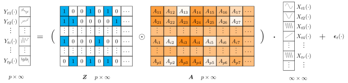
Figure 1: Sparse functional factor model. For $\boldsymbol{Z}$, the blue (or white) cells represent $1$ (or $0$). For $\boldsymbol{A}$, the darker (or lighter) shades of orange indicate larger (or smaller) values.

3.2 Gaussian Process Dynamical Model for Functional Data

Second, by projecting high-dimensional observations $\boldsymbol{Y}_{t}(\cdot)$ into low-dimensional latent functional factors $\boldsymbol{X}_{t}(\cdot)$, the sequential structure of the time series model can be captured via the factors. To model such temporal dependence of $\boldsymbol{X}_{t}(\cdot)$, we adopt a Gaussian process over time to encode historical information. In particular, we design the covariance across factors $r$ and $l$ as follows. Let $\mathcal{X}_{t}$ represent the historical information up to time $t$, and let $\mathcal{X}$ be the space containing $\{\mathcal{X}_{t}\}_{t\in{\mathbb{N}}}$. For any $u,v\in\mathcal{U}$,

$$\text{Var}\big{(}X_{tr}(u),X_{sl}(v)\big{)}=\kappa_{\mathcal{X}}(\mathcal{X}_{t-1},\mathcal{X}_{s-1})\kappa_{\mathcal{U}}(u,v)\mathbb{I}(r=l),$$ (2)

where $t$ and $s$ indicate two time stamps, $\kappa_{\mathcal{X}}$ and $\kappa_{\mathcal{U}}$ are the kernels defined on $\mathcal{X}$ and $\mathcal{U}$, respectively. $\mathbb{I}(r=l)$ is an indicator function that takes on the value of 1 if $r=l$ and 0 otherwise. $\kappa_{\mathcal{X}}$ is with respect to historical information on different periods and can be regarded as a temporal kernel. In parallel, $\kappa_{\mathcal{U}}$ can be regarded as a spatial kernel. Therefore, $\boldsymbol{X}_{r}(\cdot)=\big{(}X_{1r}(\cdot),\dots,X_{tr}(\cdot),\dots,X_{nr}(\cdot)\big{)}$ belongs a multi-task Gaussian process [15] such that for any $u_{1},\dots,u_{L}\in\mathcal{U}$, $\text{vec}\big{(}\boldsymbol{X}_{r}(u_{1},\dots,u_{L})\big{)}\sim\text{Normal}(\boldsymbol{0},\boldsymbol{\Sigma}_{\mathcal{X}}\otimes\boldsymbol{\Sigma}_{\mathcal{U}}^{u})$, where $\otimes$ denotes the Kronecker product, or equivalently $\boldsymbol{X}_{r}(u_{1},\dots,u_{L})\sim\text{MatrixNormal}(\boldsymbol{0},\boldsymbol{\Sigma}_{\mathcal{U}}^{u},\boldsymbol{\Sigma}_{\mathcal{X}})$ using the matrix normal distribution [23], where $\boldsymbol{X}_{r}(u_{1},\dots,u_{L})=\big{[}X_{tr}(u_{j})\big{]}_{1\leq t\leq n,1\leq j\leq L},$ $\boldsymbol{\Sigma}_{\mathcal{X}}=\big{[}\kappa_{\mathcal{X}}(\mathcal{X}_{t},\mathcal{X}_{s})\big{]}_{0\leq t,s\leq n-1},$ and $\boldsymbol{\Sigma}_{\mathcal{U}}^{u}=\big{[}\kappa_{\mathcal{U}}(u_{i},u_{j})\big{]}_{1\leq i,j\leq L}.$ In Appendix B, we demonstrate the detailed relationship between the multi-task Gaussian process and the matrix normal distribution. In the context of literature, the $n$-task Gaussian process is used to refer to the multiple outputs generated by the model, each of which corresponds to a specific timestamp in our time series setting. For the convenience of expression, we denote the presented multi-task Gaussian process as

$$\boldsymbol{X}_{r}(\cdot)\sim\text{MTGP}\big{(}\boldsymbol{0},\kappa_{\mathcal{U}}(\cdot,\cdot),\kappa_{\mathcal{X}}(\cdot,\cdot)\big{)}.$$ (3)

It is worth noting that the latent factors $\boldsymbol{X}_{1},\dots,\boldsymbol{X}_{r},\dots$ are not mutually independent, because they share the temporal kernel $\kappa_{\mathcal{X}}$ with respect to $\mathcal{X}_{t-1}$ that contains common historical information across factors till period $t-1$. Therefore, the multi-task Gaussian process can measure the similarity and dependence across periods. Moreover, in our setting, the temporal kernel used for prediction depends solely on past information $\mathcal{X}_{t-1}$ rather than current information $\mathcal{X}_{t}$. This approach allows for a forward-looking prediction framework based on historical data only.

The proposed model can be regarded as a functional version of the Gaussian process dynamical model [24]. See their connections in Appendix C. There are several advantages of using the proposed model to capture the temporal dependence of functional time series. First, the temporal kernel and spatial kernel are separable, providing us with a closed form and computational convenience. Moreover, since the temporal kernel is related to the entire historical information instead of the latest state only, the model can be non-Markovian. For example, we can define the temporal kernel as $\kappa(\mathcal{X}_{t-1},\mathcal{X}_{s-1})=\alpha_{1}\int\boldsymbol{X}_{t-1}(u)^{T}\boldsymbol{X}_{s-1}(u)du+\alpha_{2}\int\boldsymbol{X}_{t-2}(u)^{T}\boldsymbol{X}_{s-2}(u)du,$ to incorporate features from the last two periods. Finally, using the kernel trick, we can introduce nonlinearity by setting a nonlinear kernel function. This paves the way for us to construct deep kernels, which will be discussed in Section 3.3.

3.3 Deep Temporal Kernels

Finally, to capture the complicated nonlinear latent temporal structure, we employ deep neural networks to construct the kernel function. However, in order to use deep kernels for functional time series, we need two extra steps compared to standard deep kernels [25, 26, 27, 28, 29, 30]. (i) As $\boldsymbol{X}_{t}(\cdot)$ is a continuous process on $\mathcal{U}$, a mapping function $F:\mathcal{F}\rightarrow{\mathbb{R}}^{d}$ is required to map the infinite-dimensional Gaussian processes to $d$-dimensional vectors, where $\mathcal{F}$ is the space of continuous functions defined on $\mathcal{U}$. Various approaches can be used for this mapping function, including pre-specified basis expansion, data-dependent basis expansion (such as functional principal component analysis and its dynamic variants [31, 32]), adaptive functional neural network [33], or even simply $\boldsymbol{X}_{t}(u_{0},\dots,u_{L})$ with $u_{0},\dots,u_{L}\in\mathcal{U}$. (ii) The $d$-dimensional vectors serve as inputs for deep neural networks, and the outputs generated by these networks are then employed to construct kernel functions. Specifically, we first transform the input vector as

$$\boldsymbol{h}_{t}=H\big{(}F(\boldsymbol{X}_{t-1}),F(\boldsymbol{X}_{t-2}),\dots)\big{)},$$ (4)

where $\boldsymbol{X}_{t-1}=\big{(}X_{t-1,1},\dots,X_{t-1,r}\dots\big{)}^{\mbox{$\scriptscriptstyle T$}}$, $F$ is the mapping function, and $H$ is a sequential deep learning framework.Various deep neural network architectures can be utilized for this purpose, such as LSTM, GRU, and attention mechanisms, which have demonstrated their effectiveness in modeling complex patterns and dependencies. Since the inputs for the temporal kernels are ordered sequences from $\mathcal{X}_{0}$ to $\mathcal{X}_{n-1}$, we should use unidirectional deep neural networks instead of bidirectional networks. We then use the transformed representations $\boldsymbol{h}_{t}$ and $\boldsymbol{h}_{s}$ to construct a kernel function

$$\kappa_{\mathcal{X}}(\mathcal{X}_{t-1},\mathcal{X}_{s-1})=\kappa(\boldsymbol{h}_{t},\boldsymbol{h}_{s}),$$ (5)

where $\kappa(\cdot,\cdot)$ is a suitable kernel function, such as the squared exponential kernel or the Ornstein–Uhlenbeck kernel. We note that the temporal kernel is related to the historical values of all the relevant factors and shared across factors.

In summary, using the functional version of the sparse factor model, sequential deep learning kernel, and Gaussian process dynamical model presented above, we define a probabilistic generative model for high-dimensional functional time series and name it as deep functional factor model, DF²M. To mitigate overfitting, one can apply spectrum normalization, which effectively instills a Lipschitz condition into the neural networks according to [34]. This suggests that the inputs for $\kappa$ could reflect the distance between $\mathcal{X}_{t-1}$ and $\mathcal{X}_{s-1}$.

4 Bayesian Inference for DF²M

4.1 Sparse Variational Inference

We adopt the variational inference framework to infer the proposed DF²M. This algorithm approximates the posterior probability by maximizing the evidence lower bound (ELBO), which is equivalent to minimizing the Kullback–Leibler (KL) divergence between a variational distribution and true posterior distribution [35]. For DF²M, with mean-field factorization assuming independence among the variational distributions for latent variables, its ELBO can be expressed as

$$\begin{split}\text{ELBO}=&\operatorname{E}_{q}\Big{[}\log p(\boldsymbol{Z}\mid\alpha)p(\boldsymbol{A}\mid\sigma_{A})\prod_{t=1}^{n}p\big{(}\boldsymbol{Y}_{t}(\cdot)\mid\boldsymbol{X}_{t}(\cdot),\boldsymbol{Z},\boldsymbol{A}\big{)}\prod_{r\geq 1}p\big{(}\boldsymbol{X}_{r}(\cdot)\mid\kappa_{\mathcal{X}},\kappa_{\mathcal{U}}\big{)}\Big{]}\\ &-\operatorname{E}_{q}\Big{[}\log q(\boldsymbol{Z})q(\boldsymbol{A})\prod_{r\geq 1}q\big{(}\boldsymbol{X}_{r}(\cdot)\big{)}\Big{]}.\end{split}$$ (6)

Using the stick-breaking representation of the Indian buffet process as in Section 2.1, we factorize the variational distribution for $\boldsymbol{Z}$ as $q(v_{j})=\text{Beta}(v_{j};\tau_{j}^{1},\tau_{j}^{0})$ and $q(Z_{tj})=\text{Bernoulli}(Z_{tj};m_{tj})$. The corresponding variational distribution for $\boldsymbol{A}$ is factorized as $q(A_{tj})=\text{Normal}(A_{tj};\eta_{tj},{\sigma}^{2}_{A,tj})$. To avoid singular matrix inversions and improve computational efficiency, we propose a sparse variational inference approach for DF²M based on [36]. Our method introduces a set of inducing variables representing the values of the latent function at a small subset of points in $\mathcal{U}$. Moreover, we adopt the approach of having common locations for the inducing variables across functional factors, as suggested by [37]. In other words, we utilize the same set of inducing points for all tasks, which can lead to further improvement in computational efficiency. Consequently, the variational distribution for multi-task Gaussian process with inducing variables is defined as,

$$q\big{(}\boldsymbol{X}_{r}(\cdot)\big{)}=p\Big{(}X_{1r}(\cdot),\dots,X_{nr}(\cdot)\mid X_{1r}(\boldsymbol{v}),\dots,X_{nr}(\boldsymbol{v}),\kappa_{\mathcal{X}},\kappa_{\mathcal{U}}\Big{)}\prod_{t=1}^{n}q\big{(}X_{tr}(\boldsymbol{v})\big{)},$$ (7)

where $\boldsymbol{v}=(v_{1},\dots,v_{K})^{\mbox{$\scriptscriptstyle T$}}$ with $v_{1},\dots,v_{K}\in\mathcal{U}$ and $K$ is the number of inducing points. We construct the variational distribution for inducing variables as $q(X_{tr}(\boldsymbol{v}))=\text{Normal}(\boldsymbol{\mu}_{tr},\boldsymbol{S}_{tr})$. It is noteworthy that the conditional prior distribution for $X_{r}(\cdot)$, i.e., the first term on the right-hand-side of equation (7), cannot be factorized as $\prod_{t=1}^{n}p\big{(}X_{tr}(\cdot)\mid X_{tr}(\boldsymbol{v})\big{)}$, because they have temporal dependence. However, benefiting from the setting of equation (7), the conditional prior distribution appears both in variational and prior distributions and hence can be cancelled. In Appendix D.1, we derive that the ELBO in equation (6) can be simplified as

$$\text{ELBO}= \sum_{t=1}^{n}\operatorname{E}_{q}\Big{[}\log p\big{(}\boldsymbol{Y}_{t}(\cdot)\mid\boldsymbol{X}_{t}(\cdot),\boldsymbol{Z},\boldsymbol{A}\big{)}\Big{]}-\text{KL}\big{[}q(\boldsymbol{Z})\parallel p(\boldsymbol{Z}\mid\alpha)\big{]}$$ (8)

$$-\text{KL}\big{[}q(\boldsymbol{A})\parallel p(\boldsymbol{A}\mid\sigma_{A})\big{]}-\sum_{r\geq 1}\text{KL}\Big{[}q\big{(}\boldsymbol{X}_{r}(\boldsymbol{v})\big{)}\parallel p\big{(}\boldsymbol{X}_{r}(\boldsymbol{v})\mid\kappa_{\mathcal{X}},\kappa_{\mathcal{U}}\big{)}\Big{]},$$

where $\boldsymbol{X}_{r}(\boldsymbol{v})=\big{(}X_{1r}(\boldsymbol{v}),\dots,X_{nr}(\boldsymbol{v})\big{)}$ with $X_{tr}(\boldsymbol{v})=\big{(}X_{tr}(v_{1}),\dots,X_{tr}(v_{K})\big{)}^{\mbox{$\scriptscriptstyle T$}}$ for $t=1,\dots,n$. Furthermore, using the formula of the KL divergence between two multivariate Gaussian distributions, we derive a closed form of the last term as

$$2\text{KL}\Big{[}q\big{(}\boldsymbol{X}_{r}(\boldsymbol{v})\big{)}\parallel p\big{(}\boldsymbol{X}_{r}(\boldsymbol{v}) \mid\kappa_{\mathcal{X}},\kappa_{\mathcal{U}}\big{)}\Big{]}=\text{trace}\Big{(}(\boldsymbol{\Sigma}_{\mathcal{X}}^{-1}\otimes{\boldsymbol{\Sigma}_{\mathcal{U}}^{vv}}^{-1})\big{(}\boldsymbol{S}_{r}+\text{vec}(\boldsymbol{\mu}_{r})\text{vec}(\boldsymbol{\mu}_{r})^{\mbox{$\scriptscriptstyle T$}}\big{)}\Big{)}$$

$$+K\log|\boldsymbol{\Sigma}_{\mathcal{X}}|+n\log|\boldsymbol{\Sigma}_{\mathcal{U}}^{vv}|-\sum_{t=1}^{n}\log|\boldsymbol{S}_{tr}|-nK,$$ (9)

where $\boldsymbol{\mu}_{r}=(\boldsymbol{\mu}_{1r},\dots,\boldsymbol{\mu}_{nr})$, $\boldsymbol{S}_{r}=\text{diag}(\boldsymbol{S}_{1r},\dots,\boldsymbol{S}_{nr})$, and $\boldsymbol{\Sigma}_{\mathcal{U}}^{vv}=\big{[}\kappa_{\mathcal{U}}(v_{j},v_{j})\big{]}_{1\leq i,j\leq K}.$ See Appendix D.2 for the detailed derivation.

4.2 Sampling for Variational Distribution of Factors

To optimize the variational distributions, the automatic differentiation variational inference (ADVI) algorithm [38, 35, 39] is adopted to maximize the ELBO in equation (8). To perform ADVI in our model, we need to sample $\boldsymbol{X}_{r}(\cdot)$ from its variational distribution as specified in equation (7). However, though this distribution is Gaussian conditional on $\boldsymbol{X}_{r}(\boldsymbol{v})$, directly sampling from a $nL\times nL$ matrix is computationally expensive. To address this issue, we take advantage of the separability of the temporal and spatial kernels as described in Section 3.2, and propose the following method to accelerate the computation of the ELBO. For any $\boldsymbol{u}=(u_{1},\dots,u_{L})^{\mbox{$\scriptscriptstyle T$}}$ with $u_{1},\dots,u_{L}\in\mathcal{U}$ being the observation points in $\mathcal{U}$, we first partition the spatial covariance matrix for $\boldsymbol{X}(\boldsymbol{u},\boldsymbol{v})$ into a blockwise matrix$\begin{bmatrix}\boldsymbol{\Sigma}_{\mathcal{U}}^{uu}&{\boldsymbol{\Sigma}_{\mathcal{U}}^{uv}}\\ {\boldsymbol{\Sigma}_{\mathcal{U}}^{uv}}^{\mbox{$\scriptscriptstyle T$}}&\boldsymbol{\Sigma}_{\mathcal{U}}^{vv}\end{bmatrix},$ where $\boldsymbol{\Sigma}_{\mathcal{U}}^{uu}=\big{[}\kappa_{\mathcal{U}}(u_{i},u_{j})\big{]}_{1\leq i,j\leq L},$ and $\boldsymbol{\Sigma}_{\mathcal{U}}^{uv}=\big{[}\kappa_{\mathcal{U}}(u_{i},v_{j})\big{]}_{1\leq i\leq L,1\leq j\leq K}.$

Proposition 1 (Posterior Mean)

The mean function of the posterior for $X_{tr}(\cdot)$ is solely dependent on the variational mean of $\boldsymbol{X}_{tr}(\boldsymbol{v})$, the inducing variables at time $t$. That is, for any $\boldsymbol{u}$

$$\operatorname{E}\big{(}X_{tr}(\boldsymbol{u})\big{)}=\boldsymbol{\Sigma}_{\mathcal{U}}^{uv}{\boldsymbol{\Sigma}_{\mathcal{U}}^{vv}}^{-1}\boldsymbol{\mu}_{tr}.$$ (10)

It means that for MTGP, the variational mean is independent of the inducing variables at timestamps other than the current one. See also a similar proposition for Gaussian process regression in [15].

Proposition 2 (Posterior Variance)

The variance function of the posterior for $\boldsymbol{X}_{r}(\cdot)$ contains two parts. For any $\boldsymbol{u}$,

$$\operatorname{Var}_{q}\Big{[}\operatorname{vec}\big{(}\boldsymbol{X}_{r}(\boldsymbol{u})\big{)}\Big{]}=(I\otimes\boldsymbol{\Sigma}_{\mathcal{U}}^{uv}{\boldsymbol{\Sigma}_{\mathcal{X}}^{vv}}^{-1})\operatorname{diag}(\boldsymbol{S}_{1r},\dots,\boldsymbol{S}_{nr})+\boldsymbol{\Sigma}_{\mathcal{X}}\otimes(\boldsymbol{\Sigma}_{\mathcal{U}}^{uu}-\boldsymbol{\Sigma}_{\mathcal{U}}^{uv}{\boldsymbol{\Sigma}_{\mathcal{U}}^{vv}}^{-1}{\boldsymbol{\Sigma}_{\mathcal{U}}^{uv}}^{\mbox{$\scriptscriptstyle T$}}).$$

The first part is solely dependent on the variational variance of $\boldsymbol{X}_{tr}(\boldsymbol{v})$, and the second part is independent of the variational distributions of all inducing variables. In particular, the first part corresponds to a group of independent Gaussian processes such that $\tilde{\boldsymbol{X}}_{tr}^{(1)}(\boldsymbol{u})\sim\text{Normal}(\boldsymbol{\Sigma}_{\mathcal{U}}^{uv}{\boldsymbol{\Sigma}_{\mathcal{X}}^{vv}}^{-1}\boldsymbol{\mu}_{tr},\boldsymbol{\Sigma}_{\mathcal{U}}^{uv}{\boldsymbol{\Sigma}_{\mathcal{X}}^{vv}}^{-1}\boldsymbol{S}_{tr})$ for any $\boldsymbol{u}$, and $\tilde{\boldsymbol{X}}_{r}^{(2)}(\cdot)$ is a zero-mean multi-task Gaussian process such that $\tilde{\boldsymbol{X}}_{r}^{(2)}(\boldsymbol{u})\sim\text{MatrixNormal}(\boldsymbol{0},\boldsymbol{\Sigma}_{\mathcal{U}}^{uu}-\boldsymbol{\Sigma}_{\mathcal{U}}^{uv}{\boldsymbol{\Sigma}_{\mathcal{U}}^{vv}}^{-1}{\boldsymbol{\Sigma}_{\mathcal{U}}^{uv}}^{\mbox{$\scriptscriptstyle T$}},\boldsymbol{\Sigma}_{\mathcal{X}})$ for any $\boldsymbol{u}$. Therefore, benefiting from Propositions 1 and 2, we can decompose ${\boldsymbol{X}}_{r}(\cdot)=\tilde{\boldsymbol{X}}_{r}^{(1)}(\cdot)+\tilde{\boldsymbol{X}}_{r}^{(2)}(\cdot)$ under the variational distribution. $\tilde{\boldsymbol{X}}_{r}^{(1)}(\cdot)$ can be efficiently sampled because it only depends on inducting variables at the same period instead of all periods.

Proposition 3 (Irrelevance to ELBO)

Conditional on $\boldsymbol{\Sigma}_{\mathcal{X}}$ and $\boldsymbol{\Sigma}_{\mathcal{U}}$, sampling $\boldsymbol{X}_{tr}(\cdot)$ from the distribution of $\tilde{\boldsymbol{X}}_{r}^{(1)}(\cdot)$ does not alter the variational mean. Moreover, the corresponding ELBO of DF²M in equation (8) is modified only by a constant term given by

$$\frac{1}{2\sigma_{\epsilon}^{2}}\left\|\boldsymbol{Z}\odot\boldsymbol{A}\right\|_{F}^{2}\operatorname{trace}\big{[}\boldsymbol{\Sigma}_{\mathcal{X}}\big{]}\operatorname{trace}\big{[}\boldsymbol{\Sigma}_{\mathcal{U}}^{uu}-\boldsymbol{\Sigma}_{\mathcal{U}}^{uv}{\boldsymbol{\Sigma}_{\mathcal{U}}^{vv}}^{-1}{\boldsymbol{\Sigma}_{\mathcal{U}}^{uv}}^{\mbox{$\scriptscriptstyle T$}}\big{]},$$ (11)

where, for any matrix ${\bf M}=(M_{ij})$, we denote its Frobenius norm by $\|{\bf M}\|_{F}=\big{(}\sum_{i,j}M_{ij}^{2}\big{)}^{\frac{1}{2}}$.

See Appendices D.3, D.4 and D.5 for the derivations of Proposition 1, 2 and 11, respectively. Based on these propositions, we can sample $\boldsymbol{X}_{tr}(\cdot)$ from the proxy variational distribution $\text{Normal}(\boldsymbol{\Sigma}_{\mathcal{U}}^{uv}{\boldsymbol{\Sigma}_{\mathcal{X}}^{vv}}^{-1}\boldsymbol{\mu}_{tr},\boldsymbol{\Sigma}_{\mathcal{U}}^{uv}{\boldsymbol{\Sigma}_{\mathcal{X}}^{vv}}^{-1}\boldsymbol{S}_{tr})$, which relies solely on the variational distributions at time $t$. This approach provides an efficient way of computing the ELBO compared to direct sampling, which necessitates the complete Cholesky decomposition of the $nL\times nL$ matrix.

4.3 Initialization, Training and Prediction

We use the technique of ADVI to train the variational parameters of the posteriors by computing the gradient of the ELBO with respect to the parameters. The training process requires iterating through the following steps until the ELBO converges. The steps of Bayesian inference for DF²M are summarized in Algorithm 1 in Appendix E.

First, conditional on $\boldsymbol{\Sigma}_{\mathcal{X}}$, we update the variational distribution parameters $\boldsymbol{\mu}_{tr}$ and $\boldsymbol{S}_{tr}$ for inducing variables $\boldsymbol{X}_{tr}(\boldsymbol{v})$ for all $t$ and $r$, as well as other variational parameters including $\{\tau_{j}^{1},\tau_{j}^{2}\}_{1\leq j\leq M}$ and $\{m_{tj}\}_{1\leq t\leq n,1\leq j\leq M}$ for India buffet process $\boldsymbol{Z}$, $\{\eta_{tj},\sigma_{tj}^{A}\}_{1\leq t\leq n,1\leq j\leq M}$ for loading weight matrix $\boldsymbol{A}$, the idiosyncratic noise scale $\sigma_{\epsilon}$, and the parameters in spatial kernel $\kappa_{\mathcal{U}}(\cdot,\cdot)$. In this step, the gradient of ELBO is accelerated by sampling $X_{tr}(\cdot)$ independently according to Proposition 11 and the analytical expression for the KL divergence in equation (4.1).

Second, conditional on a sample of $\boldsymbol{X}_{r}(\cdot)$, we update the trainable parameters in sequential deep learning framework $H$ that constructs the temporal kernels $\kappa_{\mathcal{X}}(\cdot,\cdot)$, via the gradient of ELBO with respect to $\boldsymbol{\Sigma}_{\mathcal{X}}$. Although any mapping function $F$ can be used in our model, it is natural to choose $F\big{(}\boldsymbol{X}_{t}(\cdot)\big{)}=\boldsymbol{X}_{t}(\boldsymbol{v})$, such that there is no need to sample $\boldsymbol{X}_{r}(\cdot)$ when computing the gradient. This is inspired by the fact that the variational distribution of inducing variables can be regarded as sufficient statistics of the Gaussian processes [36].

Once we have observed the data at time $n$, we use the trained model to generate a posterior distribution, which captures our updated understanding of the underlying patterns in the data. Based on this distribution, we make a prediction for the value of the data at the next time step, $n+1$. We present the one-step ahead prediction as:

$$\bar{\boldsymbol{Y}}_{n+1}(\boldsymbol{u})=(\bar{\boldsymbol{Z}}\odot\bar{\boldsymbol{A}})\bar{\boldsymbol{X}}_{n+1}(\boldsymbol{u}),\quad\bar{X}_{n+1,r}(\boldsymbol{u})=\boldsymbol{\Sigma}_{\mathcal{U}}^{uv}{\boldsymbol{\Sigma}_{\mathcal{U}}^{vv}}^{-1}\boldsymbol{\mu}_{r}\boldsymbol{\Sigma}_{\mathcal{X}}^{-1}{\boldsymbol{\Sigma}_{\mathcal{X}}^{n+1,1:n}}^{\mbox{$\scriptscriptstyle T$}},$$ (12)

where $\bar{\boldsymbol{Y}}$ and $\bar{\boldsymbol{X}}$ represent the predictive means for the observations and factors, respectively. The terms $\bar{\boldsymbol{Z}}$ and $\bar{\boldsymbol{A}}$ are the posterior means of $\boldsymbol{Z}$ and $\boldsymbol{A}$, respectively. The component $\boldsymbol{\Sigma}_{\mathcal{X}}^{n+1,1:n}$ is a $1\times n$ matrix given by $\boldsymbol{\Sigma}_{\mathcal{X}}^{n+1,1:n}=\big{[}\kappa_{\mathcal{X}}(\mathcal{X}_{n+1},\mathcal{X}_{0}),\cdots,\kappa_{\mathcal{X}}(\mathcal{X}_{n+1},\mathcal{X}_{n})\big{]}.$ See Appendix D.6 for the derivations. By repeating this process iteratively, we can generate a sequence of predictions for future time steps, forecasting the behavior of the system over time.

(1) $Y_{tj}(\cdot)$ Functional time series observations (2) $X_{tr}(\cdot)$ Inferred functional factors (3) $\boldsymbol{\Sigma}_{\mathcal{X}}$ Temporal covariance matrices

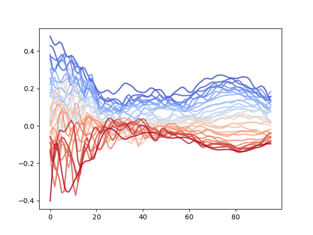
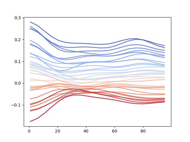
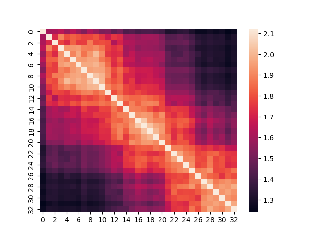
(a) Japanese Mortality

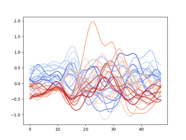
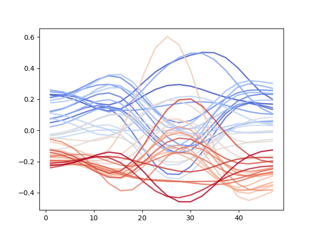
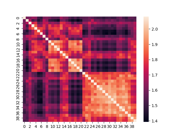
(b) Energy Consumption

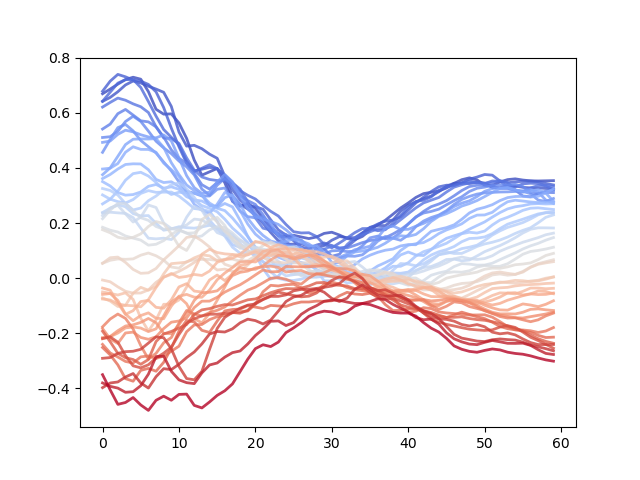
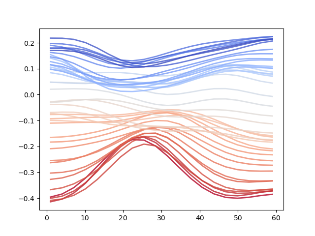
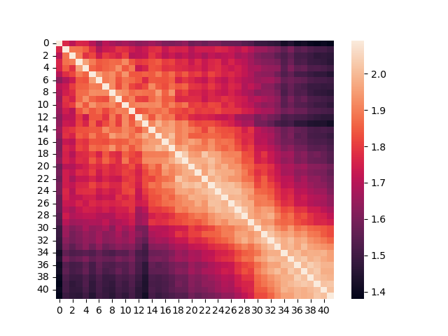
(c) Global Mortality

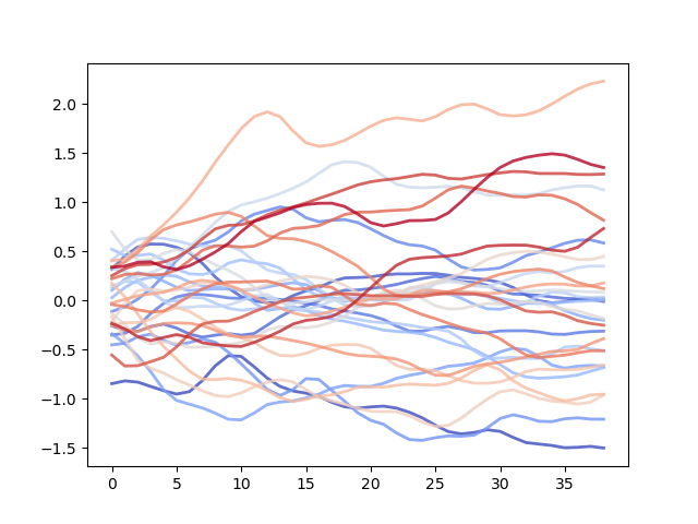
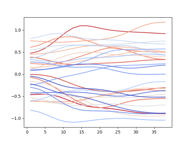
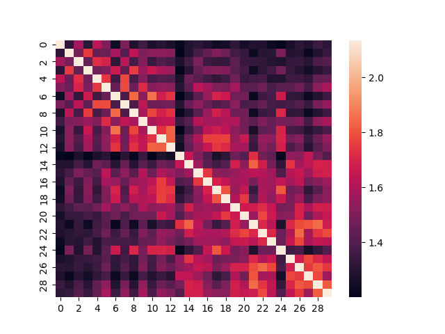
(d) Stock Intraday

Figure 3: A visualization of real datasets in the experiments. Rows 1 and 2 use a blue-to-red gradient to denote time progression, with blue for older and red for recent data. Row 3 employs brightness variations to represent covariance, with brighter areas indicating higher covariance.

5 Experiments

5.1 Datasets

We apply DF²M to four real-world datasets consisting of high-dimensional functional time series. Japanese Mortality dataset contains age-specific mortality rates for 47 Japanese prefectures ($p$=47) from 1975 to 2017, with 43 observations per prefecture ($n$=43). Energy Consumption dataset includes half-hourly measured energy consumption curves for selected London households ($p$=40) between December 2012 and January 2013 ($n$=55). Global Mortality dataset provides a broader perspective on mortality rates by including age-specific mortality data across different countries ($p$=32) from 1960 to 2010 ($n$=50). Stock Intraday dataset comprises high-frequency price observations for the S&P 100 component stocks (we removed 2 stocks with missing values, so $p$=98) in 2017. The data includes 45 trading days ($n$=45), with ten-minute resolution prices and cumulative intraday return trajectories [40]. For the preprocessing, each dataset is cleaned and transformed into an appropriate format for analysis. See Appendix F for the details. We denote the data as $\big{\{}Y_{tj}(u_{k})\big{\}}_{1\leq t\leq n,1\leq j\leq p,1\leq k\leq K}$, where $K$ is the number of observations per curve. We plot examples of functional time series for a randomly selected $j$ in Row 1 of Figure 3.

5.2 Experiment Setup and Metrics

Moreover, to assess the predictive accuracy of the proposed model, we split the data into a training set with the first $n_{1}$ periods and a test set with the last $n_{2}$ periods. We use the training set to train the parameters in the model following the steps in Section 4. Then for an integer $h>0$, we make the $h$-step-ahead prediction given the fitted model using the first $n_{1}$ periods, and then repeatedly move the training window by one period, refit the model, and make the $h$-step-ahead prediction. We compute the mean absolute prediction error (MAPE) and mean squared prediction error (MSPE) by

$$\text{MAPE}(h)\!=\!\frac{1}{M}\sum_{j=1}^{p}\sum_{k=1}^{K}\sum\limits_{\hskip 11.38092pt\mathclap{t=n_{1}+h}}^{n}\big{|}\hat{Y}_{tj}(u_{k})-Y_{tj}(u_{k})\big{|},\ \text{MSPE}(h)\!=\!\frac{1}{M}\sum_{j=1}^{p}\sum_{k=1}^{K}\sum\limits_{\hskip 11.38092pt\mathclap{t=n_{1}+h}}^{n}\big{[}\hat{Y}_{tj}(u_{k})-Y_{tj}(u_{k})\big{]}^{2},$$

where $M=Kp(n_{2}-h+1)$. In our DF²M implementation, we incorporate three cutting-edge deep learning modules: LSTM, GRU, and the self-attention mechanism. In the deep learning modules, we employ a feedforward neural network equipped with ReLU activation functions to map inputs into a designated hidden layer size. Subsequently, the transformed inputs are channeled through a time-invariant full-connected neural network, LSTM, GRU, or self-attention mechanisms, and denote them as DF²M-LIN, DF²M-LSTM, DF²M-GRU and G-ATTN, respectively. For DF²M, the outputs of deep learning modules are passed to the kernel function, while in conventional deep learning, they are converted to outputs via a linear transformation. We evaluate their performance against conventional deep learning models under the same structural setting and regulations. The optimal hyperparameters, along with a detailed description of the deep learning architecture, can be found in Appendix G. The proposed inference algorithm is used to infer DF²M and make predictions.

5.3 Empirical Results

Explainability Firstly, Row 2 of Figure 3 shows the temporal dynamic of the largest factors in the fitted models. We can observe a decreasing trend over time for the first three datasets. This is particularly valuable as these factors exhibit a clear and smooth dynamic, which can be used to explain the underlying reasons for changes over time and also to make robust predictions. Secondly, the temporal covariance matrix ($\boldsymbol{\Sigma}_{\mathcal{X}}$) can be seen in Row 3 of Figure 3. It is evident that the first three datasets exhibit stronger autocorrelation than the Stock Intraday dataset, which aligns with the intuition that financial data is generally noisier and characterized by short-term dependencies.

Furthermore, both mortality datasets display a strong autoregressive pattern, as evidenced by the large covariance values close to the diagonal. They also show a blockwise pattern, which indicates the existence of change points in 1980s. Another interesting observation is the periodic pattern in the Energy Consumption dataset, which reveals distinct patterns for weekdays and weekends during the first 21 days. This data corresponds to the first 21 days in December. In contrast, the second half of the time steps do not exhibit this pattern. This could be attributed to the Christmas holidays in London, during which the differences between weekdays and weekends are relatively smaller, as people are on holiday.

Predictive Accuracy Compared to standard deep learning models, the DF²M framework consistently outperforms other models in terms of both MSPE and MAPE across all four datasets. The only exception to this is the Stock Intraday dataset, where DF²M-ATTN and ATTN achieve similar levels of accuracy. Specifically, the DF²M-LSTM model performs exceptionally well on the Energy Consumption and Global Mortality datasets, while the DF²M-ATTN model exhibits the lowest prediction error for the Japanese Mortality dataset. These results demonstrate that the integration of an explainable structure with the nonlinearity of LSTM and attention mechanisms can significantly improve the overall performance of the model.

On the other hand, the DF²M-LIN model outperforms both DF²M-LSTM and DF²M-GRU on the Stock Intraday dataset. This can be attributed to the fact that, in the context of financial data, long-term dependencies may not be present, rendering the Markovian model more suitable for capturing the underlying dynamics. Consequently, the DF²M-LIN model emerges as a better choice for the Stock Intraday dataset. Compared to standard deep learning models with multiple layers, DF²M achieves better or comparable results, as shown in Appendix G. However, in such cases, standard deep learning models sacrifice explainability due to their utilization of a large number of layers.

Table 1: Comparision of DF²M to Standard Deep Learning Models. For formatting reasons, MAPEs are multiplied by 10, and MSPEs are multiplied by 10², except for Energy Consumption dataset.

	$h$	DF2M-LIN		LIN		DF2M-LSTM		LSTM		DF2M-GRU		GRU		DF2M-ATTN		ATTN
		MSPE	MAPE	MSPE	MAPE	MSPE	MAPE	MSPE	MAPE	MSPE	MAPE	MSPE	MAPE	MSPE	MAPE	MSPE	MAPE
Japanese   Mortality	1	4.707	1.539	7.808	2.092	3.753	1.205	4.989	1.447	4.092	1.318	8.800	1.691	3.608	1.119	13.44	3.166
	2	4.567	1.446	8.774	2.227	4.164	1.322	5.597	1.523	4.395	1.402	8.552	1.809	3.839	1.203	14.85	3.363
	3	5.623	1.635	9.228	2.313	4.513	1.427	6.501	1.684	4.898	1.537	10.41	1.865	3.985	1.264	16.17	3.546
Energy   Consm.	1	10.29	2.334	16.16	2.939	8.928	2.176	13.51	2.635	9.132	2.204	15.55	2.872	14.22	2.741	17.03	3.130
	2	17.58	3.060	18.95	3.214	11.60	2.478	19.71	3.278	15.49	2.801	24.02	3.518	18.70	3.141	17.79	3.216
	3	17.64	3.100	20.27	3.342	17.26	3.063	24.61	3.759	14.13	2.801	23.91	3.626	19.03	3.163	18.24	3.268
Global   Mortality	1	10.78	2.319	16.84	2.783	7.672	1.726	13.28	2.332	8.741	1.967	14.12	2.211	9.905	2.141	39.52	5.332
	2	9.300	2.041	18.05	2.949	8.088	1.823	16.29	2.572	8.714	1.951	15.33	2.403	10.46	2.237	41.83	5.506
	3	9.706	2.106	19.93	3.174	8.954	1.978	17.08	2.680	9.730	2.110	17.53	2.597	11.12	2.324	43.95	5.643
Stock   Intraday	1	99.58	6.424	137.5	7.896	107.5	6.741	193.3	9.281	102.5	6.675	414.0	14.12	104.2	6.695	103.4	6.579
	2	101.2	6.505	127.8	7.491	118.8	7.141	176.0	9.283	117.3	7.339	445.9	14.66	103.4	6.646	98.39	6.392
	3	89.82	6.269	139.1	7.924	113.6	7.294	213.8	10.20	95.49	6.649	427.2	14.07	93.93	6.427	91.21	6.275

6 Related Works

In the literature concerning frequentist statistical methods for high-dimensional functional time series, various approaches have been employed. For instance, [8] develop a finite-dimensional functional factor model for dimension reduction, while [2] carry out autocovariance-based dimension reduction, and [41] adopt segmentation transformation. However, all these methods use either a vector autoregressive model (VAR) or functional VAR to describe the temporal dynamics, implying linear and Markovian models. In contrast, our work is the first to propose a Bayesian model for high-dimensional functional time series that can handle nonlinear and non-Markovian dynamics. Moreover, [25, 26, 27, 28, 29, 30] use deep kernels in the Gaussian process for classification or regression tasks. Differently, we pioneer a framework that employs a deep kernel specifically for time series prediction. Lastly, [42, 24, 43] adopt MTGPs to model cross-sectional correlations among static data. Contrarily, we apply a factor model to describe cross-sectional relationships, and the temporal kernel is constructed based on the features of factors. This unique structure represents a novel contribution to the current literature.

7 Conclusion

In this paper, we present DF²M, a novel deep Bayesian nonparametric approach for discovering non-Markovian and nonlinear dynamics in high-dimensional functional time series. DF²M combines the strengths of the Indian buffet process, factor model, Gaussian process, and deep neural networks to offer a flexible and powerful framework. Our model effectively captures non-Markovian and nonlinear dynamics while using deep learning in a structured and explainable way. A potential limitation of our study lies in our reliance on simple spatial kernels, neglecting to account for the intricate relationships within the observation space $\mathcal{U}$. We leave this for future work.

Appendix

Appendix A An Introduction for Sequential Deep Learning Modules

A.1 Recurrent Neural Networks

LSTM and GRU are both types of Recurrent Neural Networks (RNNs). They are designed to address the problem of vanishing gradients of vanilla RNNs and to preserve long-term dependencies in the sequential data.

LSTM, proposed by [11], is composed of memory cells and gates that control the flow of information into and out of the memory cells. The standard structure of LSTM is composed of three types of gates: input gate, output gate and forget gate. The input gate controls the flow of new information into the memory cell, the output gate controls the flow of information out of the memory cell, and the forget gate controls the information that is removed from the memory cell. The standard structure of LSTM is defined as follows,

$$\boldsymbol{f}_{t}=\sigma(\boldsymbol{W}_{f}[\boldsymbol{h}_{t-1},\boldsymbol{x}_{t}]+\boldsymbol{b}_{f})$$

$$\boldsymbol{i}_{t}=\sigma(\boldsymbol{W}_{i}[\boldsymbol{h}_{t-1},\boldsymbol{x}_{t}]+\boldsymbol{b}_{i})$$

$$\tilde{\boldsymbol{c}}_{t}=\tanh(\boldsymbol{W}_{C}[\boldsymbol{h}_{t-1},\boldsymbol{x}_{t}]+\boldsymbol{b}_{c})$$

$${\boldsymbol{c}}_{t}=\boldsymbol{f}_{t}\odot\boldsymbol{c}_{t-1}+\boldsymbol{i}_{t}\odot\tilde{\boldsymbol{c}}_{t}$$

$$\boldsymbol{o}_{t}=\sigma(\boldsymbol{W}_{o}[\boldsymbol{h}_{t-1},\boldsymbol{x}_{t}]+\boldsymbol{b}_{o})$$

$$\boldsymbol{h}_{t}=\boldsymbol{o}_{t}\odot\tanh(\tilde{\boldsymbol{c}}_{t}),$$

where $[\boldsymbol{h}_{t-1},\boldsymbol{x}_{t}]$ is the stack of hidden state vector $\boldsymbol{h}_{t-1}$ and $\boldsymbol{x}_{t}$. $\boldsymbol{f}_{t}$, $\boldsymbol{i}_{t}$, and $\boldsymbol{o}_{t}$ are the activation vectors for forget gate, update gate, and output gate, respectively. $\tilde{\boldsymbol{c}}_{t}$ is cell input activation vector, and $c_{t}$ is cell state vector, $\sigma$ denotes sigmoid function. $\boldsymbol{W}$s and $\boldsymbol{b}$s refer to weight matrices and bias vectors to be estimated.

GRU is a simplified version of LSTM. It has two gates: update gate and reset gate. The update gate controls the flow of new information into the memory cell, while the reset gate controls the flow of information out of the memory cell. The structure of GRU is defined as follows,

$$\boldsymbol{z}_{t}=\sigma(\boldsymbol{W}_{z}[\boldsymbol{h}_{t-1},\boldsymbol{x}_{t}]+\boldsymbol{b}_{z})$$

$$\boldsymbol{r}_{t}=\sigma(\boldsymbol{W}_{r}[\boldsymbol{h}_{t-1},\boldsymbol{x}_{t}]+\boldsymbol{b}_{r})$$

$$\tilde{\boldsymbol{h}}_{t}=\tanh(\boldsymbol{W}_{h}[\boldsymbol{r}_{t}\odot\boldsymbol{h}_{t-1},\boldsymbol{x}_{t}]+\boldsymbol{b}_{h})$$

$$\boldsymbol{h}_{t}=(1-\boldsymbol{z}_{t})\odot\boldsymbol{h}_{t-1}+\boldsymbol{z}_{t}\odot\tilde{\boldsymbol{h}}_{t},$$

where $\boldsymbol{z}_{t}$ and $\boldsymbol{r}_{t}$ are the activation vectors for update gate and reset gate, respectively, and $\tilde{\boldsymbol{h}}_{t}$ is cell input activation vector.

A.2 Attention Mechanism

Attention mechanism is a deep learning model that is especially effective for sequential data prediction. It allows the model to assign different weights to different parts of the input, rather than treating them all equally. This can improve the model’s ability to make predictions by allowing it to focus on the most relevant parts of the input. The commonly used self-attention mechanism computes a weight for each element of the input, and the final output is a weighted sum of the input elements, where the weights are computed based on a query, a set of key-value pairs and a similarity function such as dot-product or MLP. The structure of standard self-attention mechanism is shown as follows,

$$\boldsymbol{q}_{t}=\boldsymbol{x}_{t}\boldsymbol{W}_{Q},\quad\boldsymbol{k}_{t}=\boldsymbol{x}_{t}\boldsymbol{W}_{K},\quad\boldsymbol{v}_{t}=\boldsymbol{x}_{t}\boldsymbol{W}_{V}$$

$$a_{t,s}=\frac{\exp(\boldsymbol{q}_{t}\cdot\boldsymbol{k}_{s}^{\top}/\sqrt{d_{k}})}{\sum_{i=1}^{T}\exp(\boldsymbol{q}_{t}\cdot\boldsymbol{k}_{i}^{\top}/\sqrt{d_{k}})},\quad\boldsymbol{h}_{t}=\sum_{s=1}^{T}a_{t,s}\boldsymbol{v}_{s},$$

where $\boldsymbol{q}_{t}$, $\boldsymbol{k}_{t}$, and $\boldsymbol{v}_{t}$ are query, key, and value vectors at time step $t$, respectively, $a_{t,s}$ is the attention value between time steps $t$ and $s$, $d_{k}$ is the dimension of the key vector, and $T$ is the total number of time steps in the sequence.

In particular, for time series modeling, the attention value should only depend on historical information rather than future information. Therefore, the attention value should be revised as

$$a_{t,s}=\frac{\exp(\boldsymbol{q}_{t}\cdot\boldsymbol{k}_{s}^{\top}/\sqrt{d_{k}})\mathds{1}_{s\leq t}}{\sum_{i=1}^{T}\exp(\boldsymbol{q}_{t}\cdot\boldsymbol{k}_{i}^{\top}/\sqrt{d_{k}})\mathds{1}_{s\leq t}},$$

We illustrate the differences between RNN and attention mechanisms in Figure A.1. In RNNs, the current state depends on the most recent state, implying a sequential dependence on past states. By contrast, attention mechanisms allow the current state to depend directly on all past states, providing a more flexible and potentially more expressive way to capture the relationships between past and current states in the time series.

[width=1.0]pictures/rnn

(a) RNN Layer

[width=1.0]pictures/attention

(b) Attention Mechanism

Figure A.1: The structures for sequential deep learning modules. In the attention mechanism, the colored links demonstrate that the current state relies exclusively on past states, ensuring that the model considers historical information without incorporating future data.

Appendix B Multi-task Gaussian Process and Matrix Normal Distribution

We first provide a brief introduction of matrix normal distribution. A random matrix $\boldsymbol{M}\in{\mathbb{R}}^{m\times n}$ is said to have a matrix normal distribution, denoted as $\boldsymbol{M}\sim\text{MatrixNormal}_{m\times n}(\boldsymbol{M}_{0},\boldsymbol{U},\boldsymbol{V})$, if its probability density function is given by

$$p(\boldsymbol{M})=\frac{\exp\left(-\frac{1}{2}\operatorname{trace}\left[\boldsymbol{V}^{-1}(\boldsymbol{M}-\boldsymbol{M}_{0})^{\top}\boldsymbol{U}^{-1}(\boldsymbol{M}-\boldsymbol{M}_{0})\right]\right)}{(2\pi)^{\frac{mn}{2}}|\boldsymbol{U}|^{\frac{n}{2}}|\boldsymbol{V}|^{\frac{m}{2}}},$$

where $\boldsymbol{M}_{0}\in{\mathbb{R}}^{m\times n}$ is the mean matrix, $\boldsymbol{U}\in{\mathbb{R}}^{m\times m}$ is a positive definite row covariance matrix, and $\boldsymbol{V}\in{\mathbb{R}}^{n\times n}$ is a positive definite column covariance matrix. Moreover, the distribution of $\operatorname{vec}(\boldsymbol{M})$ is given by

$$\operatorname{vec}(\boldsymbol{M})\sim\mathcal{N}_{mn}\left(\operatorname{vec}(\boldsymbol{M}_{0}),\boldsymbol{V}\otimes\boldsymbol{U}\right),$$

where $\mathcal{N}_{mn}(\cdot,\cdot)$ represents a multivariate normal distribution with dimension $mn$. Here, $\operatorname{vec}(\boldsymbol{M}_{0})$ is the mean vector, and the covariance matrix is formed by the Kronecker product of the row covariance matrix $\boldsymbol{V}$ and the column covariance matrix $\boldsymbol{U}$.

For any $u_{1},\dots,u_{L}\in\mathcal{U}$, given equation (2), we have $\text{vec}\big{(}\boldsymbol{X}_{r}(u_{1},\dots,u_{L})\big{)}\sim\text{Normal}(\boldsymbol{0},\boldsymbol{\Sigma}_{\mathcal{X}}\otimes\boldsymbol{\Sigma}_{\mathcal{U}}^{u})$,

where

$$\boldsymbol{X}_{r}(u_{1},\dots,u_{L})=\begin{bmatrix}X_{1r}(u_{1})&\cdots&X_{nr}(u_{1})\\ \cdots&\cdots&\cdots\cdots\\ X_{1r}(u_{L})&\cdots&X_{nr}(u_{L})\\ \end{bmatrix},$$

$$\boldsymbol{\Sigma}_{\mathcal{X}}=\begin{bmatrix}\kappa_{\mathcal{X}}(\mathcal{X}_{0},\mathcal{X}_{0})&\cdots&\kappa_{\mathcal{X}}(\mathcal{X}_{0},\mathcal{X}_{n-1})\\ \cdots&\cdots&\cdots\cdots\\ \kappa_{\mathcal{X}}(\mathcal{X}_{n-1},\mathcal{X}_{0})&\cdots&\kappa_{\mathcal{X}}(\mathcal{X}_{n-1},\mathcal{X}_{n-1})\\ \end{bmatrix},\quad\text{and}\quad\boldsymbol{\Sigma}_{\mathcal{U}}^{u}=\begin{bmatrix}\kappa_{\mathcal{U}}(u_{1},u_{1})&\cdots&\kappa_{\mathcal{U}}(u_{1},u_{L})\\ \cdots&\cdots&\cdots\cdots\\ \kappa_{\mathcal{U}}(u_{L},u_{1})&\cdots&\kappa_{\mathcal{U}}(u_{L},u_{L})\end{bmatrix}.$$

Therefore, $\boldsymbol{X}_{r}(u_{1},\dots,u_{L})\sim\text{MatrixNormal}(\boldsymbol{0},\boldsymbol{\Sigma}_{\mathcal{U}}^{u},\boldsymbol{\Sigma}_{\mathcal{X}})$.

Appendix C Functional version of Gaussian Process Dynamical Model

Following [24], we consider a nonlinear function $g$ with respect to historical information, achieved by a linear combination of nonlinear kernel function $\phi_{i}$s,

$$\boldsymbol{X}_{t}(\cdot)=g(\mathcal{X}_{t-1})=\sum_{i}\phi_{i}(\mathcal{X}_{t-1}){\boldsymbol{a}}_{i}(\cdot),$$ (C.1)

where $\mathcal{X}_{t-1}=\{\boldsymbol{X}_{t-1},\boldsymbol{X}_{t-2},\dots\}$ is the set of all historical factors till period $t-1$, $\phi_{i}$ is a nonlinear basis function with respect to $\mathcal{X}_{t-1}$, and $\boldsymbol{a}_{i}(\cdot)$ is a function defined on $\mathcal{U}$. Equivalently, the equation above can be presented as

$$\begin{bmatrix}X_{t1}(\cdot)\\ \cdots\\ X_{tr}(\cdot)\\ \cdots\end{bmatrix}=\sum_{i}\phi_{i}(\mathcal{X}_{t-1})\begin{bmatrix}{a}_{1i}(\cdot)\\ \cdots\\ {a}_{ri}(\cdot)\\ \cdots\end{bmatrix},$$

where $\boldsymbol{a}_{i}(\cdot)=\big{\{}{a}_{1i}(\cdot),{a}_{2i}(\cdot),\dots,{a}_{ri}(\cdot),\dots,\big{\}}^{\mbox{$\scriptscriptstyle T$}}$. This functional version of dynamical system corresponds to equation (3) in [24]. In analogy, the specific form of $g(\cdot)$ in equation (C.1), including the numbers of kernel functions, is incidental, and therefore can be marginalized out from a Bayesian perspective. Assigning each $a_{ri}(\cdot)$ an independent Gaussian process prior with kernel $\kappa_{\mathcal{U}}$, marginalizing over $g$ leads to equation (2), where $\kappa_{\mathcal{X}}(\mathcal{X}_{t-1},\mathcal{X}_{s-1})=\sum_{i}\big{\langle}\phi_{i}(\mathcal{X}_{t-1}),\phi_{i}(\mathcal{X}_{s-1})\big{\rangle}$.

Appendix D Technical Derivations and Proofs

D.1 Derivations for Equation (8)

Using the variational seting in equation (7), the ELBO in equation (6) can be written as

$$\text{ELBO}= \operatorname{E}_{q}\Big{[}\log p(\boldsymbol{Z}\mid\alpha)p(\boldsymbol{A}\mid\boldsymbol{\Sigma}_{A})\prod_{t=1}^{n}p\big{(}\boldsymbol{Y}_{t}(\cdot)\mid\boldsymbol{X}_{t}(\cdot),\boldsymbol{Z},\boldsymbol{A}\big{)}\prod_{r\geq 1}p\big{(}\boldsymbol{X}_{r}(\cdot)\mid\kappa_{\mathcal{X}},\kappa_{\mathcal{U}}\big{)}\Big{]}$$

$$-\operatorname{E}_{q}\Big{[}\log q(\boldsymbol{Z})q(\boldsymbol{A})\prod_{r\geq 1}q\big{(}\boldsymbol{X}_{r}(\cdot)\big{)}\Big{]}$$

$$= \operatorname{E}_{q}\big{[}\log p(\boldsymbol{Z}\mid\alpha)\big{]}-\operatorname{E}_{q}\big{[}\log q(\boldsymbol{Z})\big{]}+\operatorname{E}_{q}\big{[}\log p(\boldsymbol{A}\mid\boldsymbol{\Sigma}_{A})\big{]}-\operatorname{E}_{q}\big{[}\log q(\boldsymbol{A})\big{]}$$

$$+\sum_{t=1}^{n}\operatorname{E}_{q}\Big{[}\log p\big{(}\boldsymbol{Y}_{t}(\cdot)\mid\boldsymbol{X}_{t}(\cdot),\boldsymbol{Z},\boldsymbol{A}\big{)}\Big{]}$$

$$+\sum_{r\geq 1}\operatorname{E}_{q}\Big{[}\log p\big{(}X_{1r}(\cdot),\dots,X_{nr}(\cdot)\mid X_{1r}(\boldsymbol{v}),\dots,X_{nr}(\boldsymbol{v}),\kappa_{\mathcal{X}},\kappa_{\mathcal{U}}\big{)}$$

$$\quad\quad\quad\quad\quad\quad p\big{(}X_{1r}(\boldsymbol{v}),\dots,X_{nr}(\boldsymbol{v})\mid\kappa_{\mathcal{X}},\kappa_{\mathcal{U}}\big{)}\Big{]}$$

$$-\sum_{r\geq 1}\operatorname{E}_{q}\Big{[}\log p\big{(}X_{1r}(\cdot),\dots,X_{nr}(\cdot)\mid X_{1r}(\boldsymbol{v}),\dots,X_{nr}(\boldsymbol{v}),\kappa_{\mathcal{X}},\kappa_{\mathcal{U}}\big{)}$$

$$\quad\quad\quad\quad\quad\quad q\big{(}X_{1r}(\boldsymbol{v}),\dots,X_{nr}(\boldsymbol{v})\big{)}\Big{]}.$$

Next, we cancel the same items from the equation above to get:

$$\text{ELBO}= \operatorname{E}_{q}\big{[}\log p(\boldsymbol{Z}\mid\alpha)\big{]}-\operatorname{E}_{q}\big{[}\log q(\boldsymbol{Z})\big{]}+\operatorname{E}_{q}\big{[}\log p(\boldsymbol{A}\mid\boldsymbol{\Sigma}_{A})\big{]}-\operatorname{E}_{q}\big{[}\log q(\boldsymbol{A})\big{]}$$

$$+\sum_{t=1}^{n}\operatorname{E}_{q}\Big{[}\log p\big{(}\boldsymbol{Y}_{t}(\cdot)\mid\boldsymbol{X}_{t}(\cdot),\boldsymbol{Z},\boldsymbol{A}\big{)}\Big{]}$$

$$+\sum_{r\geq 1}\operatorname{E}_{q}\Big{[}\log p\big{(}X_{1r}(\boldsymbol{v}),\dots,X_{nr}(\boldsymbol{v})\mid\kappa_{\mathcal{X}},\kappa_{\mathcal{U}}\big{)}-\log q\big{(}X_{1r}(\boldsymbol{v}),\dots,X_{nr}(\boldsymbol{v})\big{)}\Big{]}.$$

Finally, equation (8) is obtained using the definition of KL divergence.

D.2 Derivations for Equation (4.1)

The Kullbuck–Leibler divergence between two $k$-dimensional multivariate Gaussian distribution $\mathcal{N}_{0}=\text{Normal}(\boldsymbol{m}_{0},\boldsymbol{\Sigma}_{0})$ and $\mathcal{N}_{1}=\text{Normal}(\boldsymbol{m}_{1},\boldsymbol{\Sigma}_{1})$ is defined as,

$$\text{KL}\left({\mathcal{N}}_{0}\parallel{\mathcal{N}}_{1}\right)={\frac{1}{2}}\left(\operatorname{trace}\left(\boldsymbol{\Sigma}_{1}^{-1}\boldsymbol{\Sigma}_{0}\right)-k+\left(\boldsymbol{m}_{1}-\boldsymbol{m}_{0}\right)^{\mathsf{T}}\boldsymbol{\Sigma}_{1}^{-1}\left(\boldsymbol{m}_{1}-\boldsymbol{m}_{0}\right)+\log\left({\frac{\det\boldsymbol{\Sigma}_{1}}{\det\boldsymbol{\Sigma}_{0}}}\right)\right).$$

In our settings, $\boldsymbol{v}=(v_{1},\dots,v_{K})^{\mbox{$\scriptscriptstyle T$}}$, the prior and variational distributions for $\boldsymbol{X}_{r}(\boldsymbol{v})$ are

$$p\Big{(}\text{vec}\big{(}\boldsymbol{X}_{r}(\boldsymbol{v})\big{)}\Big{)}=\text{Normal}(\boldsymbol{0},\boldsymbol{\Sigma}_{\mathcal{X}}\otimes\boldsymbol{\Sigma}_{\mathcal{U}}^{vv})$$

and

$$q\Big{(}\text{vec}\big{(}\boldsymbol{X}_{r}(\boldsymbol{v})\big{)}\Big{)}=\text{Normal}\Big{(}\begin{bmatrix}\boldsymbol{\mu}_{1r}\\ \cdots\\ \boldsymbol{\mu}_{nr}\end{bmatrix},\text{diag}(\boldsymbol{S}_{1r},\dots,\boldsymbol{S}_{nr})\Big{)},$$

respectively, where

$$\boldsymbol{\Sigma}_{\mathcal{X}}=\begin{bmatrix}\kappa_{\mathcal{X}}(\mathcal{X}_{0},\mathcal{X}_{0})&\cdots&\kappa_{\mathcal{X}}(\mathcal{X}_{0},\mathcal{X}_{n-1})\\ \cdots&\cdots&\cdots\cdots\\ \kappa_{\mathcal{X}}(\mathcal{X}_{n-1},\mathcal{X}_{0})&\cdots&\kappa_{\mathcal{X}}(\mathcal{X}_{n-1},\mathcal{X}_{n-1})\\ \end{bmatrix},\quad\boldsymbol{\Sigma}_{\mathcal{U}}^{vv}=\begin{bmatrix}\kappa_{\mathcal{U}}(v_{1},v_{1})&\cdots&\kappa_{\mathcal{U}}(v_{1},v_{K})\\ \cdots&\cdots&\cdots\cdots\\ \kappa_{\mathcal{U}}(v_{K},v_{1})&\cdots&\kappa_{\mathcal{U}}(v_{K},v_{K})\\ \end{bmatrix}.$$

Let $\boldsymbol{m}_{0}=\begin{bmatrix}\boldsymbol{\mu}_{1r}\\ \cdots\\ \boldsymbol{\mu}_{nr}\end{bmatrix}$, $\boldsymbol{m}_{1}=\boldsymbol{0}$, $\boldsymbol{\Sigma}_{0}=\text{diag}(\boldsymbol{S}_{1r},\dots,\boldsymbol{S}_{nr})$ and $\boldsymbol{\Sigma}_{1}=\boldsymbol{\Sigma}_{\mathcal{X}}\otimes\boldsymbol{\Sigma}_{\mathcal{U}}^{vv}$, we have

$$\text{trace}(\boldsymbol{\Sigma}_{1}^{-1}\boldsymbol{\Sigma}_{0})=\text{trace}\big{(}(\boldsymbol{\Sigma}_{\mathcal{X}}^{-1}\otimes{\boldsymbol{\Sigma}_{\mathcal{U}}^{vv}}^{-1})\text{diag}(\boldsymbol{S}_{1r},\dots,\boldsymbol{S}_{nr})\big{)},$$

$$\text{det}(\boldsymbol{\Sigma}_{1})=|\boldsymbol{\Sigma}_{\mathcal{X}}|^{M}|\boldsymbol{\Sigma}_{\mathcal{U}}^{vv}|^{n},\quad\text{det}(\boldsymbol{\Sigma}_{0})=\prod_{t=1}^{n}|\boldsymbol{S}_{tr}|,$$

and

$$\left(\boldsymbol{\mu}_{1}-\boldsymbol{\mu}_{0}\right)^{\mathsf{T}}\boldsymbol{\Sigma}_{1}^{-1}\left(\boldsymbol{\mu}_{1}-\boldsymbol{\mu}_{0}\right)=\text{trace}(\boldsymbol{\Sigma}_{1}^{-1}\boldsymbol{\mu}_{0}\boldsymbol{\mu}_{0}^{\mbox{$\scriptscriptstyle T$}})=\text{trace}\big{(}(\boldsymbol{\Sigma}_{\mathcal{X}}^{-1}\otimes{\boldsymbol{\Sigma}_{\mathcal{U}}^{vv}}^{-1})\text{vec}(\boldsymbol{\mu}_{r})\text{vec}(\boldsymbol{\mu}_{r})^{\mbox{$\scriptscriptstyle T$}}\big{)}.$$

Therefore,

$$2\text{KL}\big{(}q(\boldsymbol{v}_{r}) \parallel p(\boldsymbol{v}_{r}\mid\kappa_{\mathcal{X}},\kappa_{\mathcal{U}})\big{)}=\text{trace}\Big{(}(\boldsymbol{\Sigma}_{\mathcal{X}}^{-1}\otimes{\boldsymbol{\Sigma}_{\mathcal{U}}^{vv}}^{-1})\big{(}\boldsymbol{S}_{r}+\text{vec}(\boldsymbol{\mu}_{r})\text{vec}(\boldsymbol{\mu}_{r})^{\mbox{$\scriptscriptstyle T$}}\big{)}\Big{)}$$

$$+K\log|\boldsymbol{\Sigma}_{\mathcal{X}}|+n\log|\boldsymbol{\Sigma}_{\mathcal{U}}^{vv}|-\sum_{t=1}^{n}\log|\boldsymbol{S}_{tr}|-nK,$$

where $\boldsymbol{\mu}_{r}=(\boldsymbol{\mu}_{1r},\dots,\boldsymbol{\mu}_{nr})$ and $\boldsymbol{S}_{r}=\text{diag}(\boldsymbol{S}_{1r},\dots,\boldsymbol{S}_{nr})$. Moreover, to get avoid of large matrix computation, we can further simplify

$$\text{trace}\big{(}(\boldsymbol{\Sigma}_{\mathcal{X}}^{-1}\otimes{\boldsymbol{\Sigma}_{\mathcal{U}}^{vv}}^{-1})\boldsymbol{S}_{r}\big{)}=\sum_{t=1}^{n}{\Sigma_{\mathcal{X}}^{-1}}_{t,t}\text{trace}({\boldsymbol{\Sigma}_{\mathcal{U}}^{vv}}^{-1}\boldsymbol{S}_{tr}),$$

where ${\Sigma_{\mathcal{X}}^{-1}}_{t,t}$ denotes the $(t,t)$-th entry of ${\boldsymbol{\Sigma}_{\mathcal{X}}^{-1}}$ and

$$\text{trace}\big{(}(\boldsymbol{\Sigma}_{\mathcal{X}}^{-1}\otimes{\boldsymbol{\Sigma}_{\mathcal{U}}^{vv}}^{-1})\text{vec}(\boldsymbol{\mu}_{r})\text{vec}(\boldsymbol{\mu}_{r})^{\mbox{$\scriptscriptstyle T$}}\big{)}=\text{vec}({\boldsymbol{\mu}_{r}})^{\mbox{$\scriptscriptstyle T$}}\text{vec}({\boldsymbol{\Sigma}_{\mathcal{X}}^{-1}\boldsymbol{\mu}_{r}\boldsymbol{\Sigma}_{\mathcal{U}}^{-1}})=\text{trace}(\boldsymbol{\mu}_{r}^{\mbox{$\scriptscriptstyle T$}}\boldsymbol{\Sigma}_{\mathcal{U}}^{-1}\boldsymbol{\mu}_{r}\boldsymbol{\Sigma}_{\mathcal{X}}^{-1}).$$

D.3 Proof for Proposition 1

For any $\boldsymbol{u}=(u_{1},\dots,u_{L})^{\mbox{$\scriptscriptstyle T$}}$ with $u_{1},\dots,u_{L}\in\mathcal{U}$, in the prior distribution, $\text{vec}\big{(}\boldsymbol{X}_{r}(\boldsymbol{u},\boldsymbol{v})\big{)}$ is also normally distributed. We first partition the spatial covariance matrix as

$$\begin{bmatrix}\boldsymbol{\Sigma}_{\mathcal{U}}^{uu}&\boldsymbol{\Sigma}_{\mathcal{U}}^{uv}\\ \boldsymbol{\Sigma}_{\mathcal{U}}^{vu}&\boldsymbol{\Sigma}_{\mathcal{U}}^{vv}\end{bmatrix},$$

where $\boldsymbol{\Sigma}_{\mathcal{U}}^{uu}$ and $\boldsymbol{\Sigma}_{\mathcal{U}}^{vv}$ correspond to the block covariance matrix of $\boldsymbol{u}$ and $\boldsymbol{v}$, respectively, and $\boldsymbol{\Sigma}_{\mathcal{U}}^{uv}$ is the cross term. Based on this partition, using the formula of conditional multivariate Gaussian distribution, we then have

$$\operatorname{E}_{q}\Big{[}\text{vec}\big{(}\boldsymbol{X}_{r}(\boldsymbol{u})\big{)}\Big{]} =\operatorname{E}_{q}\Big{[}\operatorname{E}_{q}\big{[}\text{vec}\big{(}\boldsymbol{X}_{r}(\boldsymbol{u})\big{)}|\boldsymbol{X}_{r}(\boldsymbol{v})\big{]}\Big{]}$$

$$=\operatorname{E}_{q}\Big{[}\operatorname{E}_{p}\big{[}\text{vec}\big{(}\boldsymbol{X}_{r}(\boldsymbol{u})\big{)}|\boldsymbol{X}_{r}(\boldsymbol{v})\big{]}\Big{]}$$

$$=(\boldsymbol{\Sigma}_{\mathcal{X}}\otimes\boldsymbol{\Sigma}_{\mathcal{U}}^{uv})(\boldsymbol{\Sigma}_{\mathcal{X}}\otimes\boldsymbol{\Sigma}_{\mathcal{U}}^{vv})^{-1}\operatorname{E}_{q}\Big{[}\text{vec}(\boldsymbol{X}_{r}(\boldsymbol{v})\Big{]}$$

$$=(\boldsymbol{\Sigma}_{\mathcal{X}}\otimes\boldsymbol{\Sigma}_{\mathcal{U}}^{uv})(\boldsymbol{\Sigma}_{\mathcal{X}}^{-1}\otimes{\boldsymbol{\Sigma}_{\mathcal{U}}^{vv}}^{-1})\text{vec}(\boldsymbol{\mu}_{r})$$

$$=(I\otimes\boldsymbol{\Sigma}_{\mathcal{U}}^{uv}{\boldsymbol{\Sigma}_{\mathcal{U}}^{vv}}^{-1})\text{vec}(\boldsymbol{\mu}_{r}).$$

Therefore, $\operatorname{E}_{q}\Big{[}\text{vec}\big{(}\boldsymbol{X}_{r}(\boldsymbol{u})\big{)}\Big{]}=\boldsymbol{\Sigma}_{\mathcal{U}}^{uv}{\boldsymbol{\Sigma}_{\mathcal{U}}^{vv}}^{-1}\text{vec}(\boldsymbol{\mu}_{r})$, which means that conditional on $\boldsymbol{\Sigma}_{\mathcal{X}}$ and $\boldsymbol{\Sigma}_{\mathcal{U}}$, the mean of variational distribution are mutually independent over factors.

D.4 Proof for Proposition 2

We first derive the variance for the variational distribution of $\boldsymbol{X}_{r}(\boldsymbol{u})$. Note that

$$\operatorname{Var}_{q}\Big{[}\text{vec}\big{(}\boldsymbol{X}_{r}(\boldsymbol{u})\big{)}\Big{]} =\operatorname{Var}_{q}\Big{[}\operatorname{E}_{q}\big{[}\text{vec}\big{(}\boldsymbol{X}_{r}(\boldsymbol{u})\big{)}\mid\boldsymbol{X}_{r}(\boldsymbol{v})\big{]}\Big{]}+\operatorname{E}_{q}\Big{[}\operatorname{Var}_{q}\big{[}\text{vec}\big{(}\boldsymbol{X}_{r}(\boldsymbol{u})\mid\boldsymbol{X}_{r}(\boldsymbol{v})\big{)}\big{]}\Big{]}.$$

The first term is obviously

$$(I\otimes\boldsymbol{\Sigma}_{\mathcal{U}}^{uv}{\boldsymbol{\Sigma}_{\mathcal{X}}^{vv}}^{-1})\operatorname{diag}(\boldsymbol{S}_{1r},\dots,\boldsymbol{S}_{nr}).$$

In an analogy of proof for Proposition 1, the second term equals to

$$\boldsymbol{\Sigma}_{\mathcal{X}}\otimes\boldsymbol{\Sigma}_{\mathcal{U}}^{uu}-(\boldsymbol{\Sigma}_{\mathcal{X}}\otimes\boldsymbol{\Sigma}_{\mathcal{U}}^{uv}){(\boldsymbol{\Sigma}_{\mathcal{X}}\otimes\boldsymbol{\Sigma}_{\mathcal{U}}^{vv})}^{-1}(\boldsymbol{\Sigma}_{\mathcal{X}}\otimes\boldsymbol{\Sigma}_{\mathcal{U}}^{uv})^{\mbox{$\scriptscriptstyle T$}}$$

$$=\boldsymbol{\Sigma}_{\mathcal{X}}\otimes\boldsymbol{\Sigma}_{\mathcal{U}}^{uu}-(\boldsymbol{\Sigma}_{\mathcal{X}}\otimes\boldsymbol{\Sigma}_{\mathcal{U}}^{uv})(\boldsymbol{\Sigma}_{\mathcal{X}}^{-1}\otimes{\boldsymbol{\Sigma}_{\mathcal{U}}^{vv}}{-1})(\boldsymbol{\Sigma}_{\mathcal{X}}\otimes\boldsymbol{\Sigma}_{\mathcal{U}}^{uv})^{\mbox{$\scriptscriptstyle T$}}$$

$$=\boldsymbol{\Sigma}_{\mathcal{X}}\otimes\boldsymbol{\Sigma}_{\mathcal{U}}^{uu}-(I\otimes\boldsymbol{\Sigma}_{\mathcal{U}}^{uv}{\boldsymbol{\Sigma}_{\mathcal{U}}^{vv}}^{-1})(\boldsymbol{\Sigma}_{\mathcal{X}}\otimes\boldsymbol{\Sigma}_{\mathcal{U}}^{uv})^{\mbox{$\scriptscriptstyle T$}}$$

$$=\boldsymbol{\Sigma}_{\mathcal{X}}\otimes\boldsymbol{\Sigma}_{\mathcal{U}}^{uu}-(\boldsymbol{\Sigma}_{\mathcal{X}}\otimes\boldsymbol{\Sigma}_{\mathcal{U}}^{uv}{\boldsymbol{\Sigma}_{\mathcal{U}}^{vv}}^{-1}{\boldsymbol{\Sigma}_{\mathcal{U}}^{uv}}^{\mbox{$\scriptscriptstyle T$}}])$$

$$=\boldsymbol{\Sigma}_{\mathcal{X}}\otimes(\boldsymbol{\Sigma}_{\mathcal{U}}^{uu}-\boldsymbol{\Sigma}_{\mathcal{U}}^{uv}{\boldsymbol{\Sigma}_{\mathcal{U}}^{vv}}^{-1}{\boldsymbol{\Sigma}_{\mathcal{U}}^{uv}}^{\mbox{$\scriptscriptstyle T$}}).$$

Therefore, the variance for $\boldsymbol{X}_{r}(u)$ with variational distribution is,

$$\operatorname{Var}_{q}\Big{[}\text{vec}\big{(}\boldsymbol{X}_{r}(\boldsymbol{u})\big{)}\Big{]}=(I\otimes\boldsymbol{\Sigma}_{\mathcal{U}}^{uv}{\boldsymbol{\Sigma}_{\mathcal{X}}^{vv}}^{-1})\text{diag}(\boldsymbol{S}_{1r},\dots,\boldsymbol{S}_{nr})+\boldsymbol{\Sigma}_{\mathcal{X}}\otimes(\boldsymbol{\Sigma}_{\mathcal{U}}^{uu}-\boldsymbol{\Sigma}_{\mathcal{U}}^{uv}{\boldsymbol{\Sigma}_{\mathcal{U}}^{vv}}^{-1}{\boldsymbol{\Sigma}_{\mathcal{U}}^{uv}}^{\mbox{$\scriptscriptstyle T$}}).$$

D.5 Proof for Proposition 11

Though the model is infinite-dimensional, the inference is conducted on a finite grid of observations. Suppose $\{\boldsymbol{Y}_{t}(\cdot)\}_{1\leq t\leq n}$ have observations at points $\boldsymbol{u}$. Conditional on $\boldsymbol{\Sigma}_{\mathcal{X}}$ and $\boldsymbol{\Sigma}_{\mathcal{U}}$, in equation (8) we have

$$\sum_{t=1}^{n}\operatorname{E}_{q}\Big{[}\log p\big{(}\boldsymbol{Y}_{t}(\cdot)\mid\boldsymbol{X}_{t}(\cdot),\boldsymbol{Z},\boldsymbol{A}\big{)}\Big{]}$$

$$=\frac{1}{2\sigma_{\epsilon}^{2}}\operatorname{E}_{q}\sum_{i=1}^{p}\text{trace}\Big{[}\big{(}\boldsymbol{Y}_{i}(\boldsymbol{u})-\sum_{r}\beta_{ir}\boldsymbol{X}_{r}(\boldsymbol{u})\big{)}\big{(}\boldsymbol{Y}_{i}(\boldsymbol{u})-\sum_{r}\beta_{ir}\boldsymbol{X}_{r}(\boldsymbol{u})\big{)}^{\mbox{$\scriptscriptstyle T$}}\Big{]}+\text{constant}$$

$$=\frac{1}{2\sigma_{\epsilon}^{2}}\operatorname{E}_{q}\sum_{i=1}^{p}\sum_{r,j}\text{trace}\Big{[}\beta_{ir}\beta_{il}\boldsymbol{X}_{r}(\boldsymbol{u})\boldsymbol{X}_{l}(\boldsymbol{u})^{\mbox{$\scriptscriptstyle T$}}\Big{]}-\frac{1}{\sigma_{\epsilon}^{2}}\operatorname{E}_{q}\sum_{i=1}^{p}\sum_{r}\text{trace}\Big{[}\beta_{ir}\boldsymbol{X}_{r}(\boldsymbol{u})\boldsymbol{Y}_{i}(\boldsymbol{u})^{\mbox{$\scriptscriptstyle T$}}\Big{]}+\text{constant},$$

where $\beta_{ir}=(\boldsymbol{Z}\odot\boldsymbol{A})_{ir}$, $\boldsymbol{Y}_{i}(\boldsymbol{u})=\begin{bmatrix}Y_{1i}(u_{1})&\cdots&Y_{ni}(u_{1})\\ \cdots&\cdots&\cdots\cdots\\ Y_{1i}(u_{L})&\cdots&Y_{ni}(u_{L})\\ \end{bmatrix},$ and $\boldsymbol{X}_{r}(\boldsymbol{u})=\begin{bmatrix}X_{1r}(u_{1})&\cdots&X_{nr}(u_{1})\\ \cdots&\cdots&\cdots\cdots\\ X_{1r}(u_{L})&\cdots&X_{nr}(u_{L})\\ \end{bmatrix}.$ Using the above construction for ${\boldsymbol{X}}_{r}(\cdot)$, we also have

$$\operatorname{E}_{q}\boldsymbol{X}_{r}(\boldsymbol{u})\boldsymbol{X}_{l}(\boldsymbol{u})^{\mbox{$\scriptscriptstyle T$}}=\left\{\begin{matrix}\operatorname{E}_{q}\tilde{\boldsymbol{X}}_{r}^{(1)}(\boldsymbol{u})\tilde{\boldsymbol{X}}_{r}^{(1)}(\boldsymbol{u})^{\mbox{$\scriptscriptstyle T$}}+\operatorname{E}_{q}\tilde{\boldsymbol{X}}_{r}^{(2)}(\boldsymbol{u})\tilde{\boldsymbol{X}}_{r}^{(2)}(\boldsymbol{u})^{\mbox{$\scriptscriptstyle T$}}\quad r=l,\\ \operatorname{E}_{q}\tilde{\boldsymbol{X}}_{r}^{(1)}(\boldsymbol{u})\tilde{\boldsymbol{X}}_{l}^{(1)}(\boldsymbol{u})^{\mbox{$\scriptscriptstyle T$}}\quad\text{otherwise}.\end{matrix}\right.$$

and

$$\operatorname{E}_{q}\boldsymbol{X}_{r}(\boldsymbol{u})\boldsymbol{Y}_{i}(\boldsymbol{u})^{\mbox{$\scriptscriptstyle T$}}=\operatorname{E}_{q}\tilde{\boldsymbol{X}}_{r}^{(1)}(\boldsymbol{u})\boldsymbol{Y}_{i}(\boldsymbol{u})^{\mbox{$\scriptscriptstyle T$}},$$

because $\operatorname{E}_{q}\tilde{\boldsymbol{X}}_{r}^{(2)}(\boldsymbol{u})=\boldsymbol{0}$, where $\tilde{\boldsymbol{X}}_{r}^{(1)}(\boldsymbol{u})=\begin{bmatrix}\tilde{X}_{1r}^{(1)}(u_{1})&\cdots&\tilde{X}_{nr}^{(1)}(u_{1})\\ \cdots&\cdots&\cdots\cdots\\ \tilde{X}_{1r}^{(1)}(u_{L})&\cdots&\tilde{X}_{nr}^{(1)}(u_{L})\\ \end{bmatrix}$ and $\tilde{\boldsymbol{X}}_{r}^{(2)}(\boldsymbol{u})=\begin{bmatrix}\tilde{X}_{1r}^{(2)}(u_{1})&\cdots&\tilde{X}_{nr}^{(2)}(u_{1})\\ \cdots&\cdots&\cdots\cdots\\ \tilde{X}_{1r}^{(2)}(u_{L})&\cdots&\tilde{X}_{nr}^{(2)}(u_{L})\\ \end{bmatrix}.$

Furthermore,

$$\operatorname{E}_{q}\text{trace}\big{[}\tilde{\boldsymbol{X}}_{r}^{(2)}(\boldsymbol{u})\tilde{\boldsymbol{X}}_{r}^{(2)}(\boldsymbol{u})^{\mbox{$\scriptscriptstyle T$}}\big{]}=\text{trace}[\Sigma_{\mathcal{X}}]\text{trace}[\boldsymbol{\Sigma}_{\mathcal{U}}^{uu}-\boldsymbol{\Sigma}_{\mathcal{U}}^{uv}{\boldsymbol{\Sigma}_{\mathcal{U}}^{vv}}^{-1}{\boldsymbol{\Sigma}_{\mathcal{U}}^{uv}}^{\mbox{$\scriptscriptstyle T$}}].$$

Given the above results, we obtain that

$$\sum_{t=1}^{n}\operatorname{E}_{q}\Big{[}\log p\big{(}\boldsymbol{Y}_{t}(\cdot)\mid\boldsymbol{X}_{t}(\cdot),\boldsymbol{Z},\boldsymbol{A}\big{)}\Big{]}$$

$$=\frac{1}{2\sigma_{\epsilon}^{2}}\operatorname{E}_{q}\sum_{i=1}^{p}\sum_{r,j}\text{trace}\Big{[}\beta_{ir}\beta_{il}\boldsymbol{X}_{r}^{(1)}(\boldsymbol{u})\boldsymbol{X}_{l}^{(1)}(\boldsymbol{u})^{\mbox{$\scriptscriptstyle T$}}\Big{]}-\frac{1}{\sigma_{\epsilon}^{2}}\operatorname{E}_{q}\sum_{i=1}^{p}\sum_{r}\text{trace}\Big{[}\beta_{ir}\boldsymbol{X}_{r}^{(1)}(\boldsymbol{u})\boldsymbol{Y}_{i}(\boldsymbol{u})^{\mbox{$\scriptscriptstyle T$}}\Big{]}$$

$$\quad+\frac{1}{2\sigma_{\epsilon}^{2}}\left\|\boldsymbol{Z}\odot\boldsymbol{A}\right\|_{F}^{2}\text{trace}[\boldsymbol{\Sigma}_{\mathcal{X}}]\text{trace}[\boldsymbol{\Sigma}_{\mathcal{U}}^{uu}-\boldsymbol{\Sigma}_{\mathcal{U}}^{uv}{\boldsymbol{\Sigma}_{\mathcal{U}}^{vv}}^{-1}{\boldsymbol{\Sigma}_{\mathcal{U}}^{uv}}^{\mbox{$\scriptscriptstyle T$}}]+\text{constant}.$$

Therefore, conditional on $\boldsymbol{\Sigma}_{\mathcal{X}}$ and $\boldsymbol{\Sigma}_{\mathcal{U}}$, ELBO is irrelevant to the inter-task component $\boldsymbol{X}_{r}^{(2)}(\boldsymbol{u})$.

D.6 Derivations for Equation (12)

$\bar{\boldsymbol{Y}}_{t+1}(\boldsymbol{u})=(\bar{\boldsymbol{Z}}\odot\bar{\boldsymbol{A}})\bar{\boldsymbol{X}}_{t+1}(\boldsymbol{u})$ is obvious as the variational variables are assumed to be independent.

We first compute the predictive mean for the inducing variables at time $n+1$, $\bar{X}_{n+1,r}(\boldsymbol{v})$. In an analogy to Proposition 1, as the spatial kernel and temporal kernel are separable, we have

$$\bar{X}_{n+1,r}(\boldsymbol{v})^{\mbox{$\scriptscriptstyle T$}}=\boldsymbol{\Sigma}_{\mathcal{X}}^{n+1,1:n}\boldsymbol{\Sigma}_{\mathcal{X}}^{-1}\boldsymbol{\mu}_{r}^{\mbox{$\scriptscriptstyle T$}},$$

where $\boldsymbol{\Sigma}_{\mathcal{X}}^{n+1,1:n}=\big{[}\kappa_{\mathcal{X}}(\mathcal{X}_{n+1},\mathcal{X}_{0}),\kappa_{\mathcal{X}}(\mathcal{X}_{n+1},\mathcal{X}_{1}),\cdots,\kappa_{\mathcal{X}}(\mathcal{X}_{n+1},\mathcal{X}_{n-1}),\kappa_{\mathcal{X}}(\mathcal{X}_{n+1},\mathcal{X}_{n})\big{]}\in{\mathbb{R}}^{1\times n}.$ Moreover, we can predict $\bar{X}_{n+1,r}(\boldsymbol{u})$ by

$$\bar{X}_{n+1,r}(\boldsymbol{u})=\boldsymbol{\Sigma}_{\mathcal{U}}^{uv}{\boldsymbol{\Sigma}_{\mathcal{U}}^{vv}}^{-1}\bar{X}_{n+1,r}(\boldsymbol{v})=\boldsymbol{\Sigma}_{\mathcal{U}}^{uv}{\boldsymbol{\Sigma}_{\mathcal{U}}^{vv}}^{-1}\boldsymbol{\mu}_{r}\boldsymbol{\Sigma}_{\mathcal{X}}^{-1}{\boldsymbol{\Sigma}_{\mathcal{X}}^{n+1,1:n}}^{\mbox{$\scriptscriptstyle T$}}$$

Appendix E Algorithm of Inference

The steps of Bayesian inference for DF²M are summarized in Algorithm 1 below.

  Set up initialization of trainable parameters in deep learning models.

  repeat

1      1. Update variational distribution parameters $\boldsymbol{\mu}_{tr}$ and $\boldsymbol{S}_{tr}$ for inducing variables $\boldsymbol{X}_{tr}(\boldsymbol{v})$, along with other variational parameters,

2      2. Update trainable parameters in sequential deep learning framework $H$ using the gradient of ELBO with respect to $\boldsymbol{\Sigma}_{\mathcal{X}}$,

3

  until the convergence of the ELBO in equation (8).

Algorithm 1 Bayesian Inference for DF²M

Appendix F Dataset and Preprocessing

Japanese Mortality dataset is available at https://www.ipss.go.jp/p-toukei/JMD/index-en.html. We use log transformation and only keep the data with ages less than 96 years old. Energy Consumption dataset is available at https://data.london.gov.uk/dataset/smartmeter-energy-use-data-in-london-households. After removing samples with too many missing values, we randomly split the data into 40 groups and take the average to alleviate the impact of randomness. Global Mortality dataset downloaded from http://www.mortality.org/ contains mortality data from 32 countries, we use log transformation as well and keep the data with age less than 60 years old. Stock Intraday dataset is obtained from the Wharton Research Data Services (WRDS) database.

Appendix G Deep Learning Structures and Hyperparameters

Our deep learning model structure begins with a layer normalization process, designed to standardize the features within each individual sample in a given batch. Following this, the data is fed into a custom linear layer that implements a fully-connected layer alongside a ReLU activation function. The architecture then varies based on the specific model used, with the possibilities including a fully-connected neural network with Relu activation, LSTM, GRU, or an attention mechanism. The final component of the model is a linear layer that translates the output from the LSTM, GRU, or attention mechanism into the final predictions with the desired output size. To ensure an unbiased comparison between DF²M and conventional deep learning models, we configure both to have a hidden_size of 15 and restrict them to a single layer. For the ATTN model, we also set it to use one head.

We also run experiments using multiple layers and heads with Bayesian hyperparameter optimization and compare the results in Table F.1. Compared to standard deep learning models with multiple layers, DF²M achieves better or comparable results.

Table F.1: The comparison of DF²M to standard deep learning models with multiple layers. For formatting reasons, the standard deviations for MAPEs are multiplied by 10, and the standard deviations for MSPEs are multiplied by 10², except for Energy Consumption dataset.

	DF2M				Standard Deep learning
		$h$=1	$h$=2	$h$=3	$h$=1	$h$=2	$h$=3
Japanese   Mortality	MSPE	3.608	3.839	3.958	3.786	4.159	4.341
	MAPE	1.119	1.203	1.264	1.180	1.288	1.367
Energy   Consm.	MSPE	8.928	11.60	17.26	9.380	11.19	12.79
	MAPE	2.176	2.478	3.063	2.230	2.440	2.651
Global   Mortality	MSPE	7.672	8.088	8.954	8.196	8.755	9.322
	MAPE	1.726	1.823	1.978	1.639	1.753	1.857
Stock   Intraday	MSPE	99.58	101.2	89.82	100.0	95.68	88.52
	MAPE	6.424	6.505	6.269	6.450	6.283	6.162

We employ Bayesian hyperparameter optimization to tune the key hyperparameters of our model. The tuned hyperparameters are listed below. The best outcomes for Japanese Mortality are reached through a 3-layer LSTM model, which utilizes a dropout rate of 0.07, a learning rate of 0.0008, a weight decay coefficient of 0.0002, and a hidden size of 64. Similarly, for Energy Consumption, a 3-layer GRU model providing the best results employs a dropout rate of 0.08, a learning rate of 0.0004, a weight decay coefficient of 0.00009, and a hidden layer size of 64. In the case of Global Mortality, the best performance is achieved with a 2-layer GRU model that operates with a dropout rate of 0.33, a learning rate of 0.001, a weight decay coefficient of 0.0002, and a hidden layer size of 48. Lastly, for Stock Intraday, the best results are seen with a 5-layer model featuring a 3-head attention mechanism, with a dropout rate of 0.10, a learning rate of 0.0007, a weight decay coefficient of 0.0010, and a hidden layer size of 2.

Appendix H Standard Deviation of the Results

In parallel to the computation of MAPE and MSPE, we calculate their associated standard deviations by

$$\text{MAPE-STD}(h)\!=\!\Big{(}{\frac{1}{n_{2}-h}\sum_{t=n_{1}+h}^{n}\big{\{}\sum_{j=1}^{p}\sum_{k=1}^{K}\frac{1}{Kp}\big{|}\hat{Y}_{tj}(u_{k})-Y_{tj}(u_{k})\big{|}-\text{MAPE}(h)\big{\}}^{2}}\Big{)}^{\frac{1}{2}},$$

$$\text{MSPE-STD}(h)\!=\!\Big{(}{\frac{1}{n_{2}-h}\sum_{t=n_{1}+h}^{n}\big{\{}\sum_{j=1}^{p}\sum_{k=1}^{K}\frac{1}{Kp}\big{[}\hat{Y}_{tj}(u_{k})-Y_{tj}(u_{k})\big{]}^{2}-\text{MSPE}(h)\big{\}}^{2}}\Big{)}^{\frac{1}{2}}.$$

The findings are presented in Table H.1 below.

Table H.1: Standard deviation of DF²M and Standard Deep Learning Models. For formatting reasons, the standard deviations for MAPEs are multiplied by 10, and the standard deviations for MSPEs are multiplied by 10², except for Energy Consumption dataset.

	$h$	DF2M-LIN		LIN		DF2M-LSTM		LSTM		DF2M-GRU		GRU		DF2M-ATTN		ATTN
		MSPE	MAPE	MSPE	MAPE	MSPE	MAPE	MSPE	MAPE	MSPE	MAPE	MSPE	MAPE	MSPE	MAPE	MSPE	MAPE
		-STD	-STD	-STD	-STD	-STD	-STD	-STD	-STD	-STD	-STD	-STD	-STD	-STD	-STD	-STD	-STD
Japanese   Mortality	1	1.794	0.179	3.909	0.757	1.687	0.168	2.180	0.197	1.988	0.198	6.578	0.608	1.780	0.178	1.017	0.107
	2	1.737	0.173	4.788	0.864	1.717	0.171	2.833	0.200	2.066	0.206	5.746	0.457	1.449	0.144	1.043	0.116
	3	3.841	0.384	5.150	0.915	1.728	0.172	3.040	0.316	2.577	0.257	7.320	0.568	1.735	0.173	0.763	0.077
Energy   Consm.	1	0.841	0.841	14.91	1.354	0.724	0.724	11.39	1.039	0.679	0.679	9.683	0.833	1.029	1.029	12.47	1.104
	2	1.134	1.134	15.32	1.297	0.846	0.846	11.98	0.979	1.121	1.121	18.41	1.407	1.203	1.203	12.67	1.082
	3	1.080	1.080	16.35	1.262	1.229	1.229	12.89	1.049	0.985	0.985	13.05	0.949	1.308	1.308	12.72	1.060
Global   Mortality	1	3.519	0.351	14.03	1.514	0.686	0.068	3.484	0.546	1.088	0.108	4.108	0.238	1.379	0.137	1.483	0.103
	2	2.191	0.219	13.61	1.503	1.469	0.146	4.883	0.623	1.461	0.146	4.318	0.276	1.386	0.138	1.664	0.139
	3	2.580	0.258	14.03	1.466	2.676	0.267	4.803	0.640	2.365	0.236	5.747	0.269	1.386	0.138	2.602	0.217
Stock   Intraday	1	20.73	2.073	99.88	2.720	21.75	2.175	117.6	2.858	18.87	1.887	291.3	4.987	18.93	1.893	77.01	2.058
	2	22.27	2.227	86.99	2.361	27.17	2.717	93.25	1.823	19.63	1.963	329.2	4.917	21.25	2.125	78.82	2.124
	3	18.80	1.880	109.2	2.989	26.59	2.659	115.7	2.614	18.85	1.885	305.7	5.071	20.78	2.078	79.17	2.184

The results indicate that the DF²M-based methods exhibit a smaller or comparable standard deviation compared to other competitors.

References

- [1] Yuan Gao, Han Lin Shang, and Yanrong Yang. High-dimensional functional time series forecasting: An application to age-specific mortality rates. Journal of Multivariate Analysis, 170:232–243, 2019.
- [2] Jinyuan Chang, Cheng Chen, Xinghao Qiao, and Qiwei Yao. An autocovariance-based learning framework for high-dimensional functional time series. Journal of Econometrics, 2023.
- [3] Zhou Zhou and Holger Dette. Statistical inference for high-dimensional panel functional time series. Journal of the Royal Statistical Society Series B: Statistical Methodology, 85(2):523–549, 2023. titleTranslation:.
- [4] Yanming Guo, Yu Liu, Ard Oerlemans, Songyang Lao, Song Wu, and Michael S Lew. Deep learning for visual understanding: A review. Neurocomputing, 187:27–48, 2016. titleTranslation:.
- [5] Kaiming He, Xiangyu Zhang, Shaoqing Ren, and Jian Sun. Deep residual learning for image recognition. In 2016 IEEE Conference on Computer Vision and Pattern Recognition, pages 770–778, June 2016.
- [6] Ashish Vaswani, Noam Shazeer, Niki Parmar, Jakob Uszkoreit, Llion Jones, Aidan N Gomez, Lukasz Kaiser, and Illia Polosukhin. Attention Is All You Need. In Advances in Neural Information Processing Systems, volume 30, 2017.
- [7] Amirsina Torfi, Rouzbeh A Shirvani, Yaser Keneshloo, Nader Tavaf, and Edward A Fox. Natural language processing advancements by deep learning: A survey. arXiv preprint arXiv:2003.01200, 2020.
- [8] Shaojun Guo, Xinghao Qiao, and Qingsong Wang. Factor modelling for high-dimensional functional time series. arXiv:2112.13651, 2021.
- [9] Christoph Molnar. Interpretable Machine Learning. 2022.
- [10] Kyunghyun Cho, Bart Van Merriënboer, Dzmitry Bahdanau, and Yoshua Bengio. On the properties of neural machine translation: Encoder-decoder approaches. arXiv preprint arXiv:1409.1259, 2014.
- [11] Sepp Hochreiter and Jürgen Schmidhuber. Long short-term memory. Neural computation, 9(8):1735–1780, 1997. Publisher: MIT press.
- [12] Thomas L. Griffiths and Zoubin Ghahramani. The Indian buffet process: an introduction and review. Journal of Machine Learning Research, 12(32):1185–1224, 2011.
- [13] Christopher K Williams and Carl Edward Rasmussen. Gaussian Processes for Machine Learning. MIT Press Cambridge, 2006.
- [14] Thomas Hofmann, Bernhard Schölkopf, and Alexander J Smola. Kernel methods in machine learning. The annals of statistics, 36(3):1171–1220, 2008.
- [15] Edwin V Bonilla, Kian Chai, and Christopher Williams. Multi-task gaussian process prediction. In Advances in Neural Information Processing Systems, volume 20, 2007.
- [16] Pablo Moreno-Muñoz, Antonio Artés, and Mauricio Álvarez. Heterogeneous multi-output gaussian process prediction. In Advances in Neural Information Processing Systems, volume 31, 2018.
- [17] Bryan Lim and Stefan Zohren. Time-series forecasting with deep learning: a survey. Philosophical Transactions of the Royal Society A, 379(2194):20200209, 2021. Publisher: The Royal Society Publishing.
- [18] Yee Whye Teh, Michael I. Jordan, Matthew J. Beal, and David M. Blei. Hierarchical Dirichlet processes. Journal of the American Statistical Association, 101(476):1566–1581, 2006.
- [19] Chong Wang and David M. Blei. Truncation-free online variational inference for Bayesian nonparametric models. In Advances in Neural Information Processing Systems 25, 2012.
- [20] Michael C Hughes and Erik Sudderth. Memoized online variational inference for Dirichlet process mixture models. In Advances in Neural Information Processing Systems 26, pages 1133–1141, 2013.
- [21] Yirui Liu, Xinghao Qiao, and Jessica Lam. CATVI: Conditional and adaptively truncated variational inference for hierarchical bayesian nonparametric models. In Proceedings of the 25th International Conference on Artificial Intelligence and Statistics, pages 3647–3662, 2022.
- [22] Vincent Q. Vu and Jing Lei. Minimax sparse principal subspace estimation in high dimensions. The Annals of Statistics, 41(6):2905–2947, 2013.
- [23] A. Philip Dawid. Some matrix-variate distribution theory: notational considerations and a Bayesian application. Biometrika, 68(1):265–274, 1981.
- [24] Jack Wang, Aaron Hertzmann, and David J. Fleet. Gaussian process dynamical models. In Advances in Neural Information Processing Systems, volume 18, 2005.
- [25] Andrew Gordon Wilson, Zhiting Hu, Ruslan Salakhutdinov, and Eric P. Xing. Deep kernel learning. In Proceedings of the 19th International Conference on Artificial Intelligence and Statistics, pages 370–378, 2016.
- [26] Maruan Al-Shedivat, Andrew Gordon Wilson, Yunus Saatchi, Zhiting Hu, and Eric P. Xing. Learning scalable deep kernels with recurrent structure. The Journal of Machine Learning Research, 18(1):2850–2886, 2017.
- [27] Hui Xue, Zheng-Fan Wu, and Wei-Xiang Sun. Deep spectral kernel learning. In Proceedings of the 28th International Joint Conference on Artificial Intelligence, pages 4019–4025, 2019.
- [28] Wenliang Li, Danica J. Sutherland, Heiko Strathmann, and Arthur Gretton. Learning deep kernels for exponential family densities. In International Conference on Machine Learning, pages 6737–6746, 2019.
- [29] Joe Watson, Jihao Andreas Lin, Pascal Klink, Joni Pajarinen, and Jan Peters. Latent derivative Bayesian last layer networks. In Proceedings of The 24th International Conference on Artificial Intelligence and Statistics, pages 1198–1206, 2021.
- [30] Vincent Fortuin. Priors in Bayesian deep learning: a review. International Statistical Review, page 12502, 2022.
- [31] Neil Bathia, Qiwei Yao, and Flavio Ziegelmann. Identifying the finite dimensionality of curve time series. The Annals of Statistics, 38:3352–3386, 2010.
- [32] Siegfried Hormann, Lukasz Kidzinski, and Marc Hallin. Dynamic functional principal components. Journal of the Royal Statistical Society: Series B, 77:319–348, 2015.
- [33] Junwen Yao, Jonas Mueller, and Jane-Ling Wang. Deep Learning for Functional Data Analysis with Adaptive Basis Layers. In International Conference on Machine Learning, pages 11898–11908. PMLR, 2021.
- [34] Takeru Miyato, Toshiki Kataoka, Masanori Koyama, and Yuichi Yoshida. Spectral normalization for generative adversarial networks. In International Conference on Learning Representations, 2018.
- [35] David M. Blei, Alp Kucukelbir, and Jon D. McAuliffe. Variational inference: a review for statisticians. Journal of the American Statistical Association, 112(518):859–877, 2017.
- [36] Michalis Titsias. Variational learning of inducing variables in sparse Gaussian processes. In Proceedings of the 12th International Conference on Artificial Intelligence and Statistics, pages 567–574, April 2009. ISSN: 1938-7228.
- [37] Oliver Hamelijnck, William Wilkinson, Niki Loppi, Arno Solin, and Theodoros Damoulas. Spatio-temporal variational Gaussian processes. In Advances in Neural Information Processing Systems, volume 34, pages 23621–23633, 2021.
- [38] Alp Kucukelbir, Dustin Tran, Rajesh Ranganath, Andrew Gelman, and David M Blei. Automatic differentiation variational inference. Journal of machine learning research, 2017.
- [39] Rajesh Ranganath, Sean Gerrish, and David Blei. Black box variational inference. In Artificial Intelligence and Statistics, pages 814–822, 2014.
- [40] Lajos Horváth, Piotr Kokoszka, and Gregory Rice. Testing stationarity of functional time series. Journal of Econometrics, 179(1):66–82, 2014.
- [41] Jinyuan Chang, Qin Fang, Xinghao Qiao, and Qiwei Yao. On the Modelling and Prediction of High-Dimensional Functional Time Series.
- [42] Neil Lawrence. Gaussian process latent variable models for visualisation of high dimensional data. Advances in Neural Information Processing Systems, 16, 2003.
- [43] Michalis Titsias and Neil D. Lawrence. Bayesian Gaussian process latent variable model. In Proceedings of the 13th international conference on artificial intelligence and statistics, pages 844–851, 2010.