Eliminating Spurious Correlations from Pre-trained Models via Data Mixing

Abstract

Machine learning models pre-trained on large datasets have achieved remarkable convergence and robustness properties. However, these models often exploit spurious correlations between certain attributes and labels, which are prevalent in the majority of examples within specific categories but are not predictive of these categories in general. The learned spurious correlations may persist even after fine-tuning on new data, which degrades models’ performance on examples that do not exhibit the spurious correlation. In this work, we propose a simple and highly effective method to eliminate spurious correlations from pre-trained models. The key idea of our method is to leverage a small set of examples with spurious attributes, and balance the spurious attributes across all classes via data mixing. We theoretically confirm the effectiveness of our method, and empirically demonstrate its state-of-the-art performance on various vision and NLP tasks, including eliminating spurious correlations from pre-trained ResNet50 on Waterbirds and CelebA, adversarially pre-trained ResNet50 on ImageNet, and BERT pre-trained on CivilComments.

1 Introduction

Pre-training neural networks on large datasets allows learning new tasks quickly, and improves model robustness and uncertainty estimate (Hendrycks et al., 2019). Therefore, pre-trained models have become the de facto to obtain state-of-the-art in many vision and NLP tasks (He et al., 2017; Liu et al., 2019). However, neural networks are known to exploit spurious correlations in the training data: certain attributes that may correlate with certain categories during training, but are not predictive of the categories in general (Gururangan et al., 2018; McCoy et al., 2019). For example, if the majority of lighter images co-occur with flame, the model may learn to associate the flame with the lighter category, rather than relying on the lighter to make the prediction. Similarly, a toxicity classifier may learn to spuriously associate toxicity with the mention of certain demographics in the text. Such biases may persist during fine-tuning (Salman et al., 2022), and degrade models’ worst-group test performance on minority groups that do not exhibit the spurious correlation. This raises a key question: can we effectively eliminate spurious correlations in a pre-trained model, without having to retrain it?

There is a body of work on mitigating the effect of spurious features during training from scratch. If minority groups are known at training time, they can be upweighted or upsampled during the training to alleviate the spurious bias (Liu et al., 2021; Sagawa et al., 2019). If group labels are not available, minority groups can be estimated based on the model’s output during the training (Creager et al., 2021; Liu et al., 2021). Then, the model can be trained from scratch for the second time with minority groups upweighted (Creager et al., 2021; Liu et al., 2021; Han et al., 2022; Zhang et al., 2022).

However, it is very challenging when it comes to eliminating spurious correlation from a pre-trained model. Firstly, models are often pre-trained on very large datasets that may not be fully available afterwards for inferring minority groups. Secondly, even if the training data is available, minority groups cannot be inferred based on a pre-trained model that has already learned the spurious bias. Finally, even if minority groups are approximately inferred, eliminating spurious correlations from a pre-trained model should be done quickly on a small amount of data to be useful, while retraining the model from scratch with upweighted or upsampled minority groups is prohibitively expensive. The recent work of (Kirichenko et al., 2022) showed that retraining only the last layer of a pre-trained model on a group-balanced dataset improves the worst-group accuracy, suggesting the possibility of eliminating spurious correlation from a pre-trained model efficiently. However, in practice only a small group-balanced data can be obtained, leading to suboptimal performance, as we will confirm by our experiments.

To address the above problem, we propose a simple and highly effective method, namely Dispel, to Disassociate SPurious correlations from a pre-trained modEL. Dispel can address spurious correlations in two different scenarios, which require different treatments. In the first scenario, where the spurious attribute exists in all classes, the method mixes a small group-balanced dataset with a larger unbalanced dataset to achieve a tradeoff between group balance and sample size. In the second scenario, where the spurious correlation does not appear in all classes, the method propagates the spurious attribute to all classes by cross-class data mixing, eliminating its association with any specific class. The method’s effectiveness in both cases is supported by a theoretical analysis on a linear model.

Our extensive experiments demonstrate that Dispel, when applied to last layer retraining, achieves state-of-the-art worst-group performance on Waterbirds (Sagawa et al., 2019) and CivilComments (Borkan et al., 2019), and competitive performance on CelebA (Liu et al., 2015). Notably, unlike prior works, our method can handle scenarios where certain groups are missing in the training data. For example on CivilComments, if the non-toxic examples are missing for a particular demographic group, Dispel achieves a worst-group accuracy of 62.8%, while the best baseline only achieves 18.4%. We also show that Dispel significantly alleviates the spurious correlations (Singla et al., 2021) in an adversarially pre-trained (Madry et al., 2017) ImageNet (Deng et al., 2009) during end-to-end fine-tuning. Our effective and light-weight approach is highly beneficial for eliminating spurious biases from models pre-trained on large dataset, and only requires a small number of group-labeled examples.

2 Related Work

There has been a growing body of work on mitigating spurious correlations during training models from scratch. If group labels—indicating if an example contains the spurious attribute—are available for all training data, balancing the size of the groups (Cui et al., 2019; He and Garcia, 2009), or upweighting the minority groups that do not exhibit the spurious correlations (Byrd and Lipton, 2019; Shimodaira, 2000) can be applied to improve the performance on minority groups. Additionally, robust optimization techniques such as GroupDRO (Sagawa et al., 2019) that minimizes the error on the group with the highest loss during training are shown to be effective.

In absence of group labels, several works aim to infer the group labels. These methods use information such as misclassification (Liu et al., 2021), representation clusters (Zhang et al., 2022), Invariant Risk Minimization (Arjovsky and Bottou, 2017; Creager et al., 2021), and uncertainty (Han et al., 2022) of examples during the training, to approximately find the group labels, then retrain the model with upweighting (Liu et al., 2021), contrastive learning (Zhang et al., 2022), or mixing-up inputs and reweighted labels based on uncertainty (Han et al., 2022). In (Nam et al., 2020) two models are trained simultaneously, where the second model is trained while upweighting mistakes of the first model. (Nam et al., 2022) uses semi-supervised learning which leverages the group-labeled validation data to infer the training groups. However, such methods cannot infer group information from a pre-trained model that has already learned the spurious correlation, and hence are not applicable to pre-trained models. Moreover, starting the training process from scratch is computationally prohibitive and disregards the advantages offered by a pre-trained model.

Recently, Deep Feature Reweighting (DFR) (Kirichenko et al., 2022) showed that retraining only the last layer of a pre-trained model on a group-balanced subset can improve the worst-group accuracy. However, DFR falls short in situations where the group-labeled data is limited. Moreover, DFR cannot effectively eliminate a spurious correlation if the spurious attribute is not present in all groups. In contrast, our method overcomes these limitations and provides a comprehensive solution.

3 Problem Formulation

Consider a dataset consisting of examples of the form $(\bm{x},a,y)$, where $\bm{x}\in\mathcal{X}$ is the feature (e.g., an image), $a\in\mathcal{A}$ is an attribute (e.g., whether the image contains flame), and $y\in\mathcal{Y}$ represents the label (e.g., main object category). Each example $(\bm{x},a,y)$ belongs to a group $g\in\mathcal{G}$, which is represented by the combination of attributes and labels $(a,y)$. As $a$ can take multiple values, there can be multiple groups within the same class. An attribute $a$ is called spurious when it exhibits a strong correlation with a certain category in the dataset, which does not hold in general. A model trained on data with spurious correlation is likely to learn such correlation and make predictions based on it, which leads to low test accuracy on minority groups where such correlation does not exist.

Given a pre-trained model that has already learned a spurious correlation between attribute $a_{spu}$ and a label $y$, our goal is to mitigate this correlation by fine-tuning for a few epochs on a small dataset. Note that, when we use the term ‘fine-tuning’, without specifying, we refer to either last layer retraining or fine-tuning the entire network. Formally, our goal is to improve the model’s worst-group test accuracy in classes that contain $a_{spu}$:

$$\min_{g\in\mathcal{G}^{\prime}}\mathbb{E}[\mathbbm{1}_{f(x)=y}|g],$$ (1)

where $\mathcal{G}^{\prime}$ is set of groups in the classes within which the spurious attribute exists. For instance, if $flame$ only exists in $lighter$ class, $lighter$ is the only class that is affected by $flame$ and $\mathcal{G}^{\prime}=\{(flame,lighter),(no~{}flame,lighter)\}$. We note that our objective is more general than that of existing works, which only study the case where $a_{spu}$ exists in all classes (Liu et al., 2021; Sagawa et al., 2019; Nam et al., 2022; Zhang et al., 2022). In many real-world scenarios, spurious attribute only exists in some classes. In such cases, groups in classes that do not contain the spurious attribute, e.g., $(no~{}flame,purse)$, may have low test accuracy that is not attributed to the spurious feature $flame$. Improving the accuracy of such groups is beyond the scope of eliminating spurious correlation.

4 Eliminating Spurious Correlations from Pre-trained Models

4.1 Motivation

Our method can eliminate spurious correlations in two different scenarios. We start by providing two concrete examples to illustrate our motivation, and then formally present our method.

Scenario 1: When the spurious attribute exists in all classes. Consider a dataset of face images, with spurious attributes $male/female$ and labels $blond/dark$. Hence, there are four groups $male/female\times blond/dark$. If we have the group label for all the examples, we can upsample or subsample certain groups to make the four groups balanced. However, obtaining group information is expensive in practice. Nonetheless, a small group-balanced subset of data (denoted by $\mathcal{D}_{\text{BA}}$) is usually available or can be obtained by examining the group information of a small number of examples. However, fine-tuning the model on this dataset alone may result in poor generalization, due to the small sample size. We show that mixing $\mathcal{D}_{\text{BA}}$ with a larger but usually unbalanced data (denoted by $\mathcal{D}_{\text{FT}}$) that exhibit spurious correlation, allows balancing the spurious feature in all classes while leveraging the rich features contained in the $\mathcal{D}_{\text{FT}}$. In doing so, we can achieve a tradeoff between group balance and small sample size.

Scenario 2: When the spurious attribute does not exist in all classes. Consider the $lighter-flame$ example where the spurious attribute $flame$ only appears in the $lighter$ class. In this case, we can combine images of lighters with a flame ($\mathcal{D}_{\text{BA}}$), with images from all other classes in the fine-tuning dataset $\mathcal{D}_{\text{FT}}$. This propagates the spurious attribute to all classes, making it no longer associated with any specific class.

Input : fine-tuning data $\mathcal{D}_{\text{FT}}$ , group balanced data $\!\mathcal{D}_{\text{BA}}$, Model $\!f_{pre}$, params $\alpha,s$.

// $\mathcal{D}_{\text{FT}},\mathcal{D}_{\text{BA}}$ consist of either the inputs or embeddings of $\!f_{pre}$.

for $y\in\mathcal{Y}$ do

      $\mathcal{C}_{y}\leftarrow\{(\bm{x},y)|(\bm{x},y)\in\mathcal{D}_{\text{BA}}\}$

Initialize $\mathcal{D}_{\text{Mixed}}\leftarrow\mathcal{D}_{\text{FT}}$

for $(\bm{x},y)\in\mathcal{D}_{\text{Mixed}}$ do

       $\pi\sim\text{Bernoulli}(\alpha)$

       if $\pi=1$ then

             if $\mathcal{C}_{y}=\emptyset$ then

                   select $\bm{x}^{\prime}\!\!\in\!\mathcal{D}_{\text{BA}}\!$ uniformly at random

            else

                   select $\bm{x}^{\prime}\!\in\mathcal{C}_{y}\!$ uniformly at random

            $\bm{x}\leftarrow(1-s)\bm{x}+s\bm{x}^{\prime}$

return fine-tuned model $f_{pre}$ on $\mathcal{D}_{\text{Mixed}}$

Algorithm 1 Disassociating SPurious correlations from a pre-trained modEL (Dispel)

Notably, in Scenario 1, we only need to mix examples from $\mathcal{D}_{\text{FT}}$ and $\mathcal{D}_{\text{BA}}$ within each class, while in Scenario 2, we need cross-class mixing between $lighter$ and other classes. We also note that the fine-tuning data $\mathcal{D}_{\text{FT}}$ is typically smaller than the data used for pre-training, but larger than the group-balanced data $\mathcal{D}_{\text{BA}}$.

4.2 Balancing the Spurious Attribute in All Classes by Mixing Inputs or Embeddings

Formal definitions of $\mathcal{D}_{\text{FT}}$ and $\mathcal{D}_{\text{BA}}$. Based on discussions in the previous section, we define $\mathcal{D}_{\text{BA}}$ as a small dataset that contains an equal number of examples from all groups that contain the spurious attribute. In cases such as the $lighter$-$flame$ example, $\mathcal{D}_{\text{BA}}$ would only contain examples from $(flame,lighter)$ since the spurious attribute $flame$ only appears in class $lighter$. We use $\mathcal{D}_{\text{FT}}$ to denote the imbalanced fine-tuning data that we have, which is usually much larger than $\mathcal{D}_{\text{BA}}$ but smaller than the pre-training dataset.

Disassociating SPurious correlations from a pre-trained modEL (Dispel). Our method mixes examples from $\mathcal{D}_{\text{BA}}$ with examples from $\mathcal{D}_{\text{FT}}$ to create a new dataset $\mathcal{D}_{\text{Mixed}}$ where the spurious attribute is distributed in a more balanced way. We note that, given a pre-trained model, our method can be applied to either (1) retraining the last layer, where we let $\mathcal{D}_{\text{FT}}$ and $\mathcal{D}_{\text{BA}}$ be sets of embeddings generated by the pre-trained model, and retrain the last layer on the mixed embeddings; or (2) fine-tuning the entire network, where we let $\mathcal{D}_{\text{FT}}$ and $\mathcal{D}_{\text{BA}}$ be the original inputs, and fine-tune the entire model. The parameter $s$ controls the weights used for calculating the weighted average of two examples. Additionally, we introduce the parameter $\alpha$, which represents the probability of mixing two examples. This allows for a more fine-grained control of the extent of mixing the two datasets and improves the performance particularly when dealing with more complex spurious correlations or situations such as Scenario 2, where cross-class mixing is needed. However, in many other cases in our experiments, simply setting $\alpha$ to 1 and tuning the parameter $s$ is sufficient.

4.3 Theoretical Justification of Mixing $\mathcal{D}_{\text{FT}}$ and $\mathcal{D}_{\text{BA}}$ through a Study of Linear Regression

Next, we theoretically confirm the necessity of our method in both scenarios, through a study of linear regression.

4.3.1 Trading off between balancing the spurious attribute and overfitting noise

First, we provide theoretical justification of our method in Scenario 1, where the spurious attribute exists in all classes (Section 4.1). If we view the embeddings $\bm{x}$ in the analysis below as embeddings generated by a pre-trained encoder, it directly illustrates the case where we apply Dispel to retrain the last linear layer on the mixed embeddings. Thus, it provides theoretical insights that support our later experimental results in Section 5. We will demonstrate that, with an appropriate choice of hyperparameter $s$, minimizing the training loss on $\mathcal{D}_{\text{Mixed}}$ leads to better worst-group performance compared to either the large biased dataset $\mathcal{D}_{\text{FT}}$ or the small balanced dataset $\mathcal{D}_{\text{BA}}$.

We first define a family of data distributions $\mathcal{P}(\mu)$ parameterized by $\mu$ where each example $(\bm{x},y,a)$ is generated by sampling the label $y$ uniformly from $\{1,-1\}$, and the spurious attribute $a$ uniformly from $\{1,-1\}$ with $\Pr(a=y)=\mu$ and $\Pr(a=-y)=1-\mu$. If $\mu>1/2$, then the attribute $a=1$ is spuriously correlated with label $1$ while $a=-1$ is spuriously correlated with label $-1$. Given $y,a$, the input $\bm{x}=[x_{1},x_{2},\bm{\xi}]^{T}\in\mathbbm{R}^{d}$ is sampled as: $x_{1}\sim\mathcal{N}(y,\sigma_{1}^{2})$, $x_{2}\sim\mathcal{N}(a,\sigma_{2}^{2})$, $\bm{\xi}\sim\mathcal{N}(0,\frac{\sigma_{\xi}^{2}}{d-2}\bm{I}_{d-2})$. The first two coordinates of $\bm{x}$ encode the label and spurious attributes information, respectively. The remaining $d-2$ coordinates represent random input noise. We note that our analysis can generalize to cases where there are multiple feature vectors for core and spurious attributes.

$\mathcal{D}_{\text{FT}}$ comprises of $n$ examples randomly drawn from $\mathcal{P}_{spu}\coloneqq\mathcal{P}(p)$ where $p>\frac{1}{2}$. This dataset exhibits spurious correlations, with the majority groups being $(a=1,y=1)$ and $(a=-1,y=-1)$ while the other two groups are considered minorities. $\mathcal{D}_{\text{BA}}$ consists of $m$ examples from $\mathcal{P}_{balanced}\coloneqq\mathcal{P}(\frac{1}{2})$. $\mathcal{D}_{\text{Mixed}}$ is the dataset constructed in Algorithm 1 with hyperparameters $\alpha$ and $s$.

We train a linear model with parameters $\bm{w}\in\mathbbm{R}^{d}$ on $\mathcal{D}_{\text{Mixed}}$ by minimizing the MSE loss with $l_{2}$ regularization. Let $\mathcal{L}^{train}$ be the training loss and $\bm{w}^{*}$ be the minimizer. Let $\hat{\mathbbm{E}}$ denote the empirical expectation, then

$$\bm{w}^{*}=\operatorname*{arg\,min}_{\bm{w}\in\mathbbm{R}^{d}}\mathcal{L}^{train}(\bm{w}),~{}~{}\text{where}~{}~{}\mathcal{L}^{train}(\bm{w})\coloneqq\hat{\mathbbm{E}}_{(\bm{x},y)\in\mathcal{D}_{\text{Mixed}}}[(\bm{x}^{\top}\bm{w}-y)^{2}]+\lambda\|\bm{w}\|^{2}.$$

We are interested in the worst-group test loss on the minority groups where $a\neq y$:

$$\mathcal{L}^{test}_{wg}(\bm{w}^{*})\coloneqq\mathbbm{E}_{(\bm{x},y,a)}[(\bm{x}^{\top}\bm{w}^{*}-y)^{2}|a\neq y].$$

For simplicity, we assume that $\sigma_{2}=0$. To obtain a closed-form expression for $\mathcal{L}^{test}_{wg}(\bm{w}^{*})$, we examine the high-dimensional asymptotic limit where $n$, $d$, and $m$ tend to infinity. To account for the small size of $\mathcal{D}_{\text{BA}}$, we assume that $\frac{n}{d}\rightarrow\infty$, while $\frac{d}{m}\rightarrow\infty$, ensuring that $m$ is much smaller than $n$. Additionally, we assume that $\sigma_{\xi}\rightarrow\infty$, while $\frac{\sigma_{\xi}^{2}}{m}$ remains constant at $r$. We show the closed form expression of $\mathcal{L}_{wg}^{test}$ in the following theorem when $\alpha=1$.

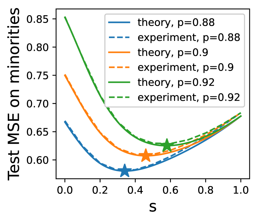
Figure 1: The worst-group test loss $\mathcal{L}_{wg}^{test}$ exhibits an initial decrease followed by an increase as $s$ increases. The optimal value of $s$, indicated by the star, increases by $p$, which represents the level of spurious correlation in the data). The solid lines correspond to Theorem 4.1 with $\sigma_{1}=0.5$, $r=4$, $\lambda=0.25$, while the dashed lines represent the experimental results obtained with $n=120000$, $d=8000$, and $m=128$. Results are average of 20 runs.

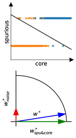
(a) $s=0$

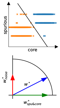
(b) $s=0.4$

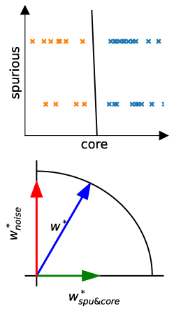
(c) $s=1$

Figure 2: A trade-off between worst-group performance and overfitting noise. Top: With increasing $s$, the spurious correlation is alleviated. The orange and blue dots represent examples from two classes in the spurious and core coordinates. The black line represents $x=-\frac{w^{*}_{2}}{w^{*}_{1}}y$, which can be seen as the decision boundary of the learned model $\bm{w}^{*}$ along the first two coordinates. Bottom: With increasing $s$, the model has a larger component in the coordinates for random noise. The normalized weights vector, its spurious and core coordinates, and its noise coordinates are shown with blue, green, and red arrows, respectively.

Theorem 4.1.

Worst-group test loss $\mathcal{L}^{test}_{wg}(\bm{w}^{*})$ has the following closed form expression:

$$\mathcal{L}^{test}_{wg}(\bm{w}^{*})\!=\!\bigg{(}\!\frac{q}{\psi_{1}\psi_{3}\!-\!\psi_{2}^{2}}\big{(}\psi_{3}\!+\!\psi_{2}\!-\!(\psi_{1}\!+\!\psi_{2})(1\!-\!s)(2p\!-\!1)\big{)}-1\!\bigg{)}^{2}\!\!\!\!+\!\sigma_{1}^{2}\big{(}\psi_{3}-\psi_{2}(1\!-\!s)(2p\!-\!1)\big{)}^{2}\!,$$

where expressions of $q,\psi_{1},\psi_{2},\psi_{3}$ are deferred to Appendix A.1.

We prove the theorem in Appendix A.1. The above expression is represented by the solid lines in Figure 2. We compare it with the results (dashed lines) obtained from experiments where $n,d,m,\sigma_{\xi}$ are finite, showing that the theoretical result closely aligns with empirical results. We observe that the best test loss on minorities is achieved with intermediate values of $s$. This intermediate value outperforms both $s=0$, which only trains on $\mathcal{D}_{\text{FT}}$, and $s=1$, which only trains on $\mathcal{D}_{\text{BA}}$. This confirms that our method can effectively improve worst-group performance, and the improvement goes beyond what is provided by $\mathcal{D}_{\text{BA}}$ alone. By comparing the test loss curves under different values of $p$, we also observe that the optimal $s$ increases as $p$ (the level of spurious correlation in $\mathcal{D}_{\text{FT}}$) increases. This is consistent with the intuition that when $\mathcal{D}_{\text{FT}}$ exhibits stronger spurious correlations, we need to bias the constructed $\mathcal{D}_{\text{Mixed}}$ more towards the balanced subset $\mathcal{D}_{\text{BA}}$ to counteract the negative impact of the spurious correlations.

To provide an intuitive explanation for why intermediate $s$ is better than $s=0$ or $s=1$, we visualize the decomposition of the trained model weights $\bm{w}^{*}$ in Figure 2. Specifically, we decompose $\bm{w}^{*}$ into two components: $\bm{w}^{*}_{s,c}$ and $\bm{w}^{*}_{noise}$. The former represents the component of $\bm{w}^{*}$ in the span of the spurious and core features, while the latter represents the component in the orthogonal complement which is the noise space. From Figure 2 we observe that as $s$ increases, the majority of examples in the two classes become less distinguishable along the spurious coordinate, resulting in the model aligning more with the core coordinate (top row). At the same time, the model also learns more noise (bottom row). Therefore, there is a trade-off between fitting noise and alleviating the spurious correlation when selecting $s$, which explains the U-shape of the minority-group test loss in Figure 2.

4.3.2 Mixing is necessary even if spurious attribute does not exist in the fine-tuning data

Next, we analyze Scenario 2 discussed in Section 4.1, where the spurious attribute $flame$ exists only in class $lighter$. In particular, we theoretically demonstrate that even if we can remove all images with the spurious attribute (i.e. lighters with flame) from the fine-tuning dataset $\mathcal{D}_{\text{FT}}$, fine-tuning on $\mathcal{D}_{\text{FT}}$ can not remove the spurious correlation learned in the pre-trained weights. Indeed, it is still necessary to mix the images of $(flame,lighter)$ with all the other classes. In the following analysis, $\bm{x}$ can be interpreted as inputs and the linear model as a representation of the entire neural network with pre-trained weights. We provide an illustrative experiments with neural networks in Appendix B.

To model data without the spurious attribute (e.g., without $flame$), we consider $\mathcal{P}_{nospu}$, which is defined the same as $\mathcal{P}$, but with the spurious attribute $a$ always equal to $0$, i.e., absent. We assume that the fine-tuning data $\mathcal{D}_{\text{FT}}$ comprises examples drawn from $\mathcal{P}_{nospu}$. We train a linear model with a bias layer given by $f(\bm{x})=\bm{w}^{\top}\bm{x}+\bm{b}$. Since the spurious attribute can only appear at the second coordinate of the inputs, given the weights of a linear model $\bm{w}$, the value of $\bm{w}^{\top}\bm{e}_{2}$, where $\bm{e}_{2}=[0,1,0,0,\dots,0]^{\top}$, indicates how much the model aligns with the spurious attribute. We fine-tune a pre-trained model $\bm{w}_{0}$ that has already learned the spurious attribute, i.e., $\bm{w}_{0}^{\top}\bm{e}_{2}>0$, by using gradient descent to minimize the MSE loss on $\mathcal{D}_{\text{FT}}$. Let $\bm{w}_{t}$ denote the weights at epoch $t$. The model only updates within the subspace spanned by the fine-tuning examples, which is orthogonal to $\bm{e}_{2}$, and thus $\bm{w}_{t}^{\top}\bm{e}_{2}$ is never affected. Therefore, we have the following proposition:

Proposition 4.2.

fine-tuning on $\mathcal{D}_{\text{FT}}$ alone cannot eliminate the spurious correlation from a pre-trained model, i.e., $\bm{w}_{t}^{\top}\bm{e}_{2}=\bm{w}_{0}^{\top}\bm{e}_{2},\forall t$.

Now let $\mathcal{D}_{\text{BA}}$ comprise $m$ examples where $a=1$ ($flame$) and $y=1$ ($lighter$). We apply Dispel as in Algorithm 1 with $\alpha=1$ to generate $\mathcal{D}_{\text{Mixed}}$. The following theorem (proved in Appendix A.2) demonstrates that fine-tuning on $\mathcal{D}_{\text{Mixed}}$ allows the model to unlearn the spurious attribute.

Theorem 4.3.

When the model is fine-tuned on $\mathcal{D}_{\text{Mixed}}$, the alignment between the weights and the spurious attribute converges to zero, i.e., $\bm{w}_{t}^{\top}\bm{e}_{2}\rightarrow 0$, as the training epoch $t\rightarrow\infty$.

5 Experiments

To evaluate the performance of our method, Dispel, we conduct two sets of experiments. First, we apply Dispel to last layer retraining while comparing it with existing methods for training from scratch to show the effectiveness of our method. Then, we apply Dispel to an adversarially pre-trained ResNet50 on Imagenet where it is necessary to fine-tune the entire model.

5.1 Dispel Applied to Last Layer Retraining (LLR) on Standard Benchmark Datasets

In the benchmark datasets we use, the spurious attribute occurs in all classes, which corresponds to Scenario 1 discussed in Section 4.1. Additionally, our application of Dispel to last layer retraining aligns with the setting that was theoretically studied in Section 4.3.1.

We use ERM to pre-train ResNet50 (He et al., 2016) and BERT (Devlin et al., 2018) on three standard vision and NLP benchmark datasets with spurious correlations, namely, Waterbirds (Sagawa et al., 2019), CelebA (Liu et al., 2015) and CivilComments (Borkan et al., 2019; Koh et al., 2021). Then we apply Dispel to retrain the last layer on mixed embeddings. The group details of the three datasets are described in Appendix C.1.

Baselines. We consider ERM, JTT (Liu et al., 2021), CnC (Zhang et al., 2022), CVaR DRO (Levy et al., 2020), SSA (Nam et al., 2022), DFR (Kirichenko et al., 2022), GroupDRO (Sagawa et al., 2019) and SUBG (Idrissi et al., 2022) as baselines. All the methods except DFR are for training from scratch. GroupDRO and SUBG require the group information for all the training examples. JTT and CnC first train a model to estimate group information based on its output, and then retrain the model with upsampling/contrastive learning. SSA trains a semi-supervised pipeline using the entire group-labeled validation data to predict group labels for training examples. On the other hand, DFR first pre-trains the model with ERM and then retrains the last layer on group-balanced data drawn from either validation data ($\text{DFR}^{\text{Val}}_{\text{Tr}}$) or training data ($\text{DFR}^{\text{Tr}}_{\text{Tr}}$). More details can be found in Appendix C.2.

Dispel Setup. We consider two settings: (1) Using fraction of validation data (✗/✓✓in Table 1): following $\text{DFR}^{\text{Val}}_{\text{Tr}}$, we retrain the last layer using half of the validation set denoted as $\mathcal{D}_{\text{Val/2}}$. We sample both $\mathcal{D}_{\text{FT}}$ and $\mathcal{D}_{\text{BA}}$ from $\mathcal{D}_{\text{Val/2}}$. For CelebA and CivilComments, $\mathcal{D}_{\text{FT}}$ is a class-balanced version of $\mathcal{D}_{\text{Val/2}}$, where examples from the smaller class are randomly upsampled to match the size of the larger class. In Waterbirds, the validation set is already group-balanced within each class. However, to showcase the effectiveness of Dispel, we need to ensure $\mathcal{D}_{\text{FT}}$ has spurious correlation. For this, we sample from $\mathcal{D}_{\text{FT}}$ in a way that the fractions of groups within each class are the same as in the training data. Specifically, we sample 948, 52, 43, 957 examples from the groups $(land,landbird)$, $(water,landbird)$, $(land,waterbird)$, and $(water,waterbird)$ respectively. To create the group-balanced $\mathcal{D}_{\text{BA}}$, we sample $l$ examples from each group in $\mathcal{D}_{\text{Val/2}}$. (2) Not using validation data (✓/✓in Table 1): We also consider the case where no validation data is used for training and $\mathcal{D}_{\text{FT}}$ and $\mathcal{D}_{\text{BA}}$ are drawn from the training set. The details are in Appendix C.3. For Waterbirds and CelebA, we set $\alpha$ to 1 and tune $s$, as this is turned out to be sufficient to get a high performance. For CivilComments, we tune both $\alpha$ and $s$ using the remaining validation data. The details and selection of other hyperparameters are described in Appendix C.3.

Table 1: Worst-group and average test accuracies of different methods. ‘Train’ column shows whether the method trains from scratch (FS) or uses last-layer retraining (LLR). Rows for LLR are highlighted in color, as LLR is faster and cheaper compared to FS. ‘Group info’ column shows if the method requires group information on training/validation data. ✓✓shows if the method also trains on validation data. For DFR and Dispel, experiments are conducted with different sizes of $\mathcal{D}_{\text{BA}}$. $l$=max means $l$ is set to the size of the smallest group in $\mathcal{D}_{\text{Val/2}}$ or training set, while $l=10/10/20$ indicates the value of $l$ on the three datasets, respectively. Best results overall are highlighted in bold, and best results for LLR are highlighted in red. Rows corresponding to settings with limited size of $\mathcal{D}_{\text{BA}}$ are highlighted in dark blue. Symbols (*) and ($\diamondsuit$) are explained in Appendix C.3

Method	Train	Group info Train/Val	Waterbirds (%)		CelebA (%)		CivilComments (%)
			Wg	Avg	Wg	Avg	Wg	Avg
ERM	FS	✗/✗	74.9	98.1	47.2	95.6	57.4	92.6
JTT		✗/✓	86.7	93.3	81.1	88.0	69.3	91.1
CnC			$88.5_{\pm 0.3}$	$90.9_{\pm 0.1}$	$88.8_{\pm 0.9}$	$89.9_{\pm 0.5}$	$68.9_{\pm 2.1}$	$81.7_{\pm 0.5}$
CVaRDRO			75.9	96.0	64.4	82.5	60.5	92.5
SSA		✗/✓✓	$89.0_{\pm 0.55}$	$92.2_{\pm 0.87}$	$89.8_{\pm 1.3}$	$92.8_{\pm 0.1}$	$69.9_{\pm 2}$	$88.2_{\pm 2}$
$\text{DFR}^{\text{Val}}_{\text{Tr}}$			$91.8_{\pm 2.6}^{*}$	$93.5_{\pm 1.4}^{*}$	$87.3_{\pm 1.0}^{*}$	$90.2_{\pm 0.8}^{*}$	$70.1_{\pm 0.8}^{\diamondsuit}$	$87.2_{\pm 0.3}^{\diamondsuit}$
Dispel	LLR	✗/✓✓  $l$=max	$92.8_{\pm 0.6}$	$94.2_{\pm 0.2}$	$88.5_{\pm 0.6}$	$91.0_{\pm 0.3}$	$71.0_{\pm 1.7}$	$89.6_{\pm 0.5}$
$\text{DFR}^{\text{Val}}_{\text{Tr}}$			$81.8_{\pm 1.0}$	$87.1_{\pm 0.8}$	$72.0_{\pm 1.3}$	$76.1_{\pm 0.9}$	$68.5_{\pm 3.0}^{\diamondsuit}$	$89.0_{\pm 1.0}^{\diamondsuit}$
Dispel	LLR	✗/✓✓  $l$=10/10/20	$89.4_{\pm 0.3}$	$93.6_{\pm 0.1}$	$86.6_{\pm 0.5}$	$90.1_{\pm 0.4}$	$70.0_{\pm 2.2}$	$89.5_{\pm 0.8}$
$\text{DFR}^{\text{Tr}}_{\text{Tr}}$			$90.4_{\pm 1.5}^{*}$	$94.1_{\pm 0.5}^{*}$	$80.1_{\pm 1.1}^{*}$	$89.7_{\pm 0.4}^{*}$	$65.0_{\pm 2.2}^{\diamondsuit}$	$90.8_{\pm 0.3}^{\diamondsuit}$
Dispel	LLR	✓/✓  $l$=max	$90.2_{\pm 0.7}$	$94.3_{\pm 0.2}$	$80.8_{\pm 1.0}$	$89.3_{\pm 0.2}$	$70.1_{\pm 0.8}$	$90.1_{\pm 0.2}$
$\text{DFR}^{\text{Tr}}_{\text{Tr}}$			$87.2_{\pm 5.1}$	$94.2_{\pm 1.0}$	$78.2_{\pm 3.8}$	$84.8_{\pm 4.0}$	$65.6_{\pm 5.4}^{\diamondsuit}$	$89.5_{\pm 1.3}^{\diamondsuit}$
Dispel	LLR	✓/✓  $l$=10/10/20	$89.2_{\pm 1.1}$	$94.0_{\pm 0.6}$	$83.1_{\pm 0.5}$	$88.0_{\pm 0.3}$	$71.2_{\pm 1.6}$	$89.9_{\pm 0.3}$
GroupDRO	FS	✓/✓	91.4	93.5	88.9	92.9	69.9	88.9
SUBG			$89.1_{\pm 1.1}$	-	$85.6_{\pm 2.3}$	-	-	-

Main Results. We consider two cases for the balanced $\mathcal{D}_{\text{BA}}$: the largest possible $\mathcal{D}_{\text{BA}}$ where $l$ is the size of the smallest group in $\mathcal{D}_{\text{Val/2}}$ or the training set ($l$=max in the table), and a very small $\mathcal{D}_{\text{BA}}$ where $l\!=\!10$ for Waterbirds and CelebA, and $l\!=\!20$ for CivilComments. Table 1 shows that Dispel achieves the best performance on both WaterBirds and CivilComments, and outperforms the second-best method (DFR) by 1.0% and 1.1%, respectively. On CelebA, Dispel outperforms DFR and achieves comparable performance to SSA, which requires an expensive semi-supervised procedure using the entire validation data. On CivilComments, Dispel achieves SOTA with only 20 examples per group in $\mathcal{D}_{\text{BA}}$.

Comparison to DFR. $\text{DFR}^{\text{Val}}_{\text{Tr}}$is the most comparable to Dispel. While $\text{DFR}^{\text{Val}}_{\text{Tr}}$retrains the last layer only on $\mathcal{D}_{\text{BA}}$, Dispel goes further by leveraging the imbalanced data $\mathcal{D}_{\text{FT}}$. Our results show that Dispel consistently outperforms $\text{DFR}^{\text{Val}}_{\text{Tr}}$, confirming the benefits of making maximal use of the available (unannotated) data. Notably, as the size of $\mathcal{D}_{\text{BA}}$ decreases (blue rows), the performance gap between Dispel and $\text{DFR}^{\text{Val}}_{\text{Tr}}$becomes more evident. On Waterbirds and CelebA, Dispel leads to an 8% and 15% improvement in the worst-group accuracy. This becomes crucial in real-world scenarios where obtaining group information is expensive and the available balanced dataset is typically very small.

5.1.1 Ablation Studies

Validation vs. Training Data for $\mathcal{D}_{\text{FT}}$ and $\mathcal{D}_{\text{BA}}$. Comparing the results in Table 1 with ✗/✓✓and with ✓/✓, we observe that using validation data leads to superior performance over using validation data on Waterbirds, CelebA, and CivilComments with $l$=max. However, interestingly, the opposite is observed on CivilComments with $l=20$. Results with other values of $l$ are in Appendix D.2.

Effects of $\alpha$, $s$ and Size of $\mathcal{D}_{\text{BA}}$. On Waterbirds and CelebA, we fix $\alpha=1$ and only tune $s$. In Figure 3, we demonstrate the effect of $s$ on the worst-group accuracy. We observe that, in general, the worst-group accuracy improves and then worsens as $s$ increases, which is consistent with the theoretical result presented in Section 4.3.1. Moreover, this increasing-decreasing pattern is more evident when $l$ is smaller. This emphasizes the importance of $\mathcal{D}_{\text{FT}}$ to enrich the input features and compensate for the insufficient sample size of $\mathcal{D}_{\text{BA}}$. Figure D.7 in Appendix D.4 shows the worst-group accuracy under different combinations of $\alpha$ and $s$ on CivilComments. We observe that the best performance is achieved at intermediate $\alpha$ and $s$. In general, larger values of $l$ tend to result in better worst-group performance. However, there are exceptions, such as in the case of CelebA and CivilComments with training data (Tabels 1 and D.6).

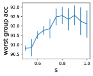
(a) Waterbirds, $l=\text{max}$

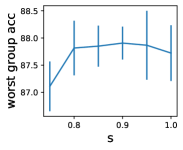
(b) CelebA, $l=\text{max}$

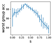
(c) Waterbirds, $l=10$

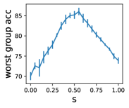
(d) CelebA, $l=10$

Figure 3: The effect of $s$, when $\alpha\!=\!1$, for different values of $l$. The worst-group accuracy initially increases and then decreases as $s$ increases, with optimal performance achieved at intermediate values of $s$. This confirms the importance of mixing $\mathcal{D}_{\text{FT}},$ $\mathcal{D}_{\text{BA}}$. The pattern is more pronounced for small $l$.

Fine-tuning the Entire Network. Dispel can be directly applied to the original inputs to fine-tune the entire network (instead of last layer). Appendix D.3 shows the results on Waterbirds and CelebA. Interestingly, on CelebA, when $\mathcal{D}_{\text{FT}}$ and $\mathcal{D}_{\text{BA}}$ are drawn from the training data, it leads to better performance (c.f. Table D.5 vs Table 1 with $l\!=\!10$). However, there is no benefit in other settings.

5.1.2 Dispel is the Only Effective Method on Severely Biased Dataset with Missing Groups

Table 2: Dispel significantly improves the performance when one group is completely missing.

Method	Wg (%)	Avg (%)
Pre-trained (ERM)	17.9	90.7
GroupDRO	$18.4_{\pm 0.1}$	$90.0_{\pm 0.05}$
DFR	$18.2_{\pm 0.4}$	$90.2_{\pm 0.1}$
$\mathcal{D}_{\text{FT}}$ alone	$21.8_{\pm 0.1}$	$91.0_{\pm 0.1}$
$\mathcal{D}_{\text{BA}}$ alone	$1.8_{\pm 0.2}$	$12.6_{\pm 4.2}$
Dispel	$62.8_{\pm 0.6}$	$91.6_{\pm 0.1}$

We conducted experiments on a modified CivilComments dataset to demonstrate the effectiveness of our method on extremely biased training data where the minority group is completely missing. Following (Koh et al., 2021), we consider the 4 non-overlapping groups $(black,not~{}toxic)$, $(not~{}black,not~{}toxic)$, $(black,toxic)$ and $(not~{}black,toxic)$. Additionally, we remove the group $(black,not~{}toxic)$ from the training set which results in strong spurious correlation between attribute $black$ and label $toxic$. The model pre-trained on such dataset for 5 epochs has an accuracy of 97.2% on group $(black,toxic)$ while only 17.3% on group $(black,not~{}toxic)$.

To apply Dispel, we let $\mathcal{D}_{\text{BA}}$ include data only from the group $(black,toxic)$. Table 2 compares Dispel to GroupDRO and DFR (both with only the three available groups). Further details can be found in Appendix D.5. We observe that both GroupDRO and DFR fail drastically due to the lack of one group. In contrast, our method significantly improves the worst-group accuracy to $62.8$%, whereas either $\mathcal{D}_{\text{FT}}$ or $\mathcal{D}_{\text{BA}}$ alone achieves a low accuracy. This result emphasizes the importance of our method in dealing with extreme bias in data. The high level reason why our method works is that it brings the feature Black to class $not~{}toxic$, where it is originally missing, through mixing examples, thus effectively creating the missing group $(black,not~{}toxic)$.

5.2 Dispel Applied to an Adversarially Pre-trained Model on ImageNet

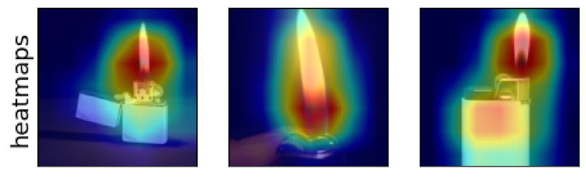
$\mathcal{D}_{\text{FT}}$ only

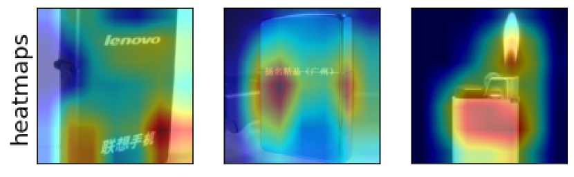
Dispel

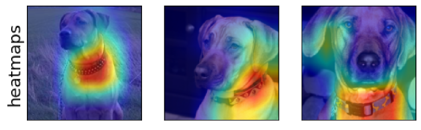
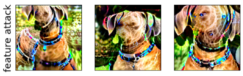
$\mathcal{D}_{\text{FT}}$ only

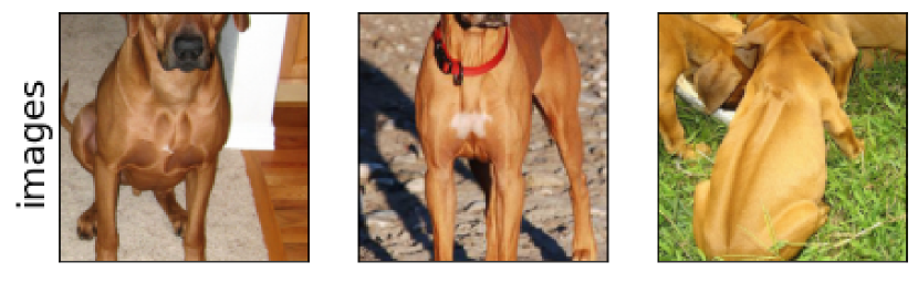
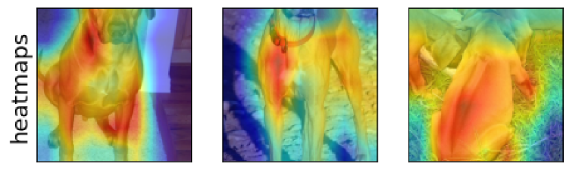
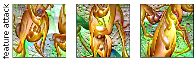
Dispel

Figure 4: The two figures on the left depict the attribute whose absence most commonly leads to wrong prediction in class $lighter$, for models trained using $\mathcal{D}_{\text{FT}}$ and Dispel. Evidently, the attribute is no longer correlated to $flame$ after Dispel is applied. The two figures on the right illustrate the same for class $rhodesian~{}ridgeback$, where Dispel alleviates the spurious correlation between the attribute $collar$ and the class, but $\mathcal{D}_{\text{FT}}$ cannot. Visualization for pre-trained models is in Appendix E.5.

Adversatrial training is prone to learning spurious correlations (Singla et al., 2021), such as those between the $flame$ attribute and the $lighter$ class, and between the $collar$ attribute and the $Rhodesian~{}ridgeback$ class on ImageNet (Deng et al., 2009). We employ our method to eliminate such spurious correlations from a ResNet-50 model adversarially pre-trained on ImageNet. Note that in this experiment, we apply Dispel to fine-tuning the entire model rather than last layer retraining, as it is necessary to preserve adversarial performance. For more details, please refer to Appendix E.1 and Table E.9. Since in this dataset the spurious correlations do not occur in all classes, the setting falls into Scenario 2 discussed in Section 4.1.

We first consider eliminating the learned spurious correlation between $flame$ and $lighter$. We construct $\mathcal{D}_{\text{FT}}$ by removing images that are highly likely to contain flames utilizing Barlow (Singla et al., 2021) (details in Appendix E.2) and then sampling 200 images per class. For $\mathcal{D}_{\text{BA}}$, we use the 180 images from the $(flame,lighter)$ group. Due to the impracticality of checking all images for flames, we assume no images with flames exist in other classes. This assumption while not entirely accurate, suffices to demonstrate our method’s effectiveness. Then the groups are $(flame,lighter)$, $(no~{}flame,lighter)$ and $(no~{}flame,y)$ for $y\neq lighter$. Hence, we only focus on the worst-group accuracy between $(flame,lighter)$ and $(no~{}flame,lighter)$, based on the objective in Section 3.

Table 3: Accuracy on the two groups in each class.

	$lighter$		$ridgeback$
	$no~{}flame$	$flame$	$no~{}collar$	$collar$
Pre-trained	13.9	76.9	27.4	70.2
DFR	23.3	45.1	32.7	41.0
$\mathcal{D}_{\text{FT}}$ only	26.4	43.6	23.5	66.8
Dispel	30.3	61.2	38.2	72.0

The model is adversatially trained during both pre-training and fine-tuning (details in Appendix E.3). Since the pre-trained model spuriously correlates $flame$ with $lighter$, the accuracy on images of lighters without flames (13.9%) is considerably lower than those with flames (76.9%). We fine-tune the model for 5 epochs using DFR and Dispel respectively, and compare the worst-group accuracy in Table 3. Our method Dispel achieves the best performance, increasing the worst-group accuracy to $30.3\%$. Notably, this is higher than that achieved by fine-tuning on $\mathcal{D}_{\text{FT}}$, which does not contain the spurious attribute. This aligns with our theoretical results in Section 4.3.2.

Visualizing the Primary Cause of Wrong Predictions. We use Barlow (Singla et al., 2021) which is a model explanation and visualization tool, to confirm that $flame$ is indeed no longer the cause of false negatives in class $lighter$. Barlow performs failure analysis by investigating which attribute’s absence leads to a model’s wrong predictions in a given class and visualizing this attribute. It displays images that exemplify this attribute (1st row), the regions within these images that best represent this attribute (2nd row), and images where the attribute is visually amplified (3rd row) (more details in Appendix E.4). Figure E.8 reveals that the absence of flame is the main reason that the pre-trained model makes wrong predictions for lighter images. Figure 4 (left) presents the results for the model fine-tuned on $\mathcal{D}_{\text{FT}}$, revealing that the primary reason still relates to the presence of a flame, albeit in conjunction with other attributes. In contrast, our method results in the primary cause of wrong predictions not visually resembling a flame (Figure 4, second from left).We show similar results for removing the spurious correlation between $collar$ and $Rhodesian~{}Ridgeback$, in Table 3 and Figures E.9, 4(c) and 4(d) in Appendix E.5.

6 Conclusion

We proposed Dispel to effectively eliminate spurious correlations from a pre-trained model. Dispel makes the most out of a small group-balanced data, by mixing it’s examples with a larger data without group labels. We proved the effectiveness of Dispel through a theoretical analysis on linear models. Our experiments showed that this simple method performs surprisingly well on many datasets. Specifically, by training a linear layer on the representations of a pre-trained model on Waterbirds, CelebA, and CivilComments, Dispel achieves a competitive or even better performance than expensive methods that eliminate the spurious bias during the training. We also showed the effectiveness of Dispel in mitigating spurious correlations from an adversarially trained model on ImageNet. Our method is well-suited for real-world scenarios where pre-trained models are widely used but are biased, and obtaining group information is expensive.

Limitation and Broader Impact. Our method requires a group-labeled data, although this requirement can be minimal as shown in experiments. We believe our method has no negative social impact and instead fosters fairness and promotes equity across applications by mitigating bias in ML models.

Appendix A Theoretical Analysis

A.1 Proof of Theorem 4.1

We study ridge regression with parameter $\lambda$. To simplify the analysis, we consider the asymptotic regime where $n,d,m\rightarrow\infty$, $n/d\rightarrow\infty$ and $d/m\rightarrow\infty$. We also assume $\sigma_{\xi}^{2}\rightarrow\infty$ while $\frac{\sigma_{\xi}^{2}}{m}$ remains at constant $r$. For simplicity we only consider the case where the hyperparameter $\alpha$ is set to 1.

Theorem A.1 (Theorem 4.1).

Worst-group test loss $\mathcal{L}^{test}_{wg}(\bm{w}^{*})$ has the following closed form expression:

$$\mathcal{L}^{test}_{wg}(\bm{w}^{*})\!=\!\bigg{(}\!\frac{q}{\psi_{1}\psi_{3}\!-\!\psi_{2}^{2}}\big{(}\psi_{3}\!+\!\psi_{2}\!-\!(\psi_{1}\!+\!\psi_{2})(1\!-\!s)(2p\!-\!1)\big{)}-1\!\bigg{)}^{2}\!\!\!\!+\!\sigma_{1}^{2}\big{(}\psi_{3}-\psi_{2}(1\!-\!s)(2p\!-\!1)\big{)}^{2}\!,$$

where $q\coloneqq\frac{\lambda}{s^{2}r+\lambda}$, and

$$\psi_{1}\coloneqq (1-s)^{2}(1+\sigma_{1}^{2})+2s(1-s)q+s^{2}q(1+\sigma_{1}^{2})-(1-s)^{2}(1-q)+\lambda,$$

$$\psi_{2}\coloneqq (1-s)^{2}(2p-1)+s(1-s)q(2p-1)-(1-s)^{2}(1-q)(2p-1),$$

$$\psi_{3}\coloneqq (1-s)^{2}+s^{2}q-(1-s)^{2}(1-q)(2p-1)^{2}+\lambda.$$

Notations

Let $\bm{X}\in\mathbbm{R}^{d\times n}$ collect inputs in $\mathcal{D}_{\text{FT}}$. Let $\bm{X}^{\prime}\in\mathbbm{R}^{d\times m}$ collect inputs in $\mathcal{D}_{\text{BA}}$. Remember that for each example in $\mathcal{D}_{\text{FT}}$, we sample an example from $\mathcal{D}_{\text{BA}}$ to construct $\mathcal{D}_{\text{Mixed}}$. Let $\bm{X}^{\prime\prime}\in\mathbbm{R}^{d\times n}$ collect the inputs sampled from $\mathcal{D}_{\text{BA}}$. Let $\tilde{\bm{X}}$ denote the inputs in $\mathcal{D}_{\text{Mixed}}$. Then $\tilde{\bm{X}}=(1-s)\bm{X}+s\bm{X}^{\prime\prime}$. Let $\bm{Y},\bm{Y}^{\prime},\bm{Y}^{\prime\prime}$ be the corresponding labels. Note that $\bm{Y}^{\prime\prime}=\bm{Y}$. We use $\bm{x},\bm{x}^{\prime},\bm{x}^{\prime\prime},\tilde{\bm{x}}$ for columns in $\bm{X},\bm{X}^{\prime},\bm{X}^{\prime\prime},\tilde{\bm{X}}$, respectively. We write $\bm{x}^{\prime}=\begin{bmatrix}\bm{f}^{\prime}\\ \bm{\zeta}^{\prime}\end{bmatrix}$ where $\bm{f}^{\prime}\in\mathbbm{R}^{2}$ and $\bm{\zeta}^{\prime}\in\mathbbm{R}^{d-2}$. Let $\bm{F}^{\prime}=[\bm{f}^{\prime}_{1},\bm{f}^{\prime}_{2},\dots,\bm{f}^{\prime}_{m}]$. Let $\mathcal{C}_{y}$ denote the set of indices of examples in $\mathcal{D}_{\text{BA}}$ with label $y$. Let $\mathcal{S}_{j}$ denote the set of indices of examples from $\mathcal{D}_{\text{FT}}$ that are going to be mixed up with $\bm{x}_{j}^{\prime}$.

Proposition A.2.

The following holds almost surely in the asymptotic regime we consider

$$\frac{1}{m}\bm{F}^{\prime}\bm{F}^{\prime}=\frac{1}{m}\sum_{i=1}^{m}\bm{f}_{i}^{\prime}\bm{f}_{i}^{\prime\top}=\begin{bmatrix}1+\sigma_{1}^{2}&0\\ 0&1\\ \end{bmatrix}\coloneqq\bm{G}_{core}$$ (2)

$$\forall i\neq j\in[m],~{}~{}\bm{\zeta}_{i}^{\prime\top}\bm{\zeta}_{j}^{\prime}=0$$ (3)

$$\forall i\in[m],~{}~{}\|\bm{\zeta}_{i}^{\prime}\|=\sigma_{\xi}$$ (4)

$$\frac{1}{n}\bm{X}\bm{X}^{\top}=\frac{1}{n}\sum_{i=1}^{n}\bm{x}\bm{x}^{\top}=\begin{bmatrix}\bm{G}_{spu}&\bm{0}\\ \bm{0}&\frac{\sigma_{\xi}^{2}}{d-2}\bm{I}_{d-2}\end{bmatrix},\text{ where }~{}~{}\bm{G}_{spu}\coloneqq\begin{bmatrix}1+\sigma_{1}^{2}&2p-1\\ 2p-1&1\end{bmatrix}$$

$$\frac{m}{n}\sum_{i\in\mathcal{S}_{j}}\bm{x}_{i}=\begin{bmatrix}y_{j}^{\prime}\\ y_{j}^{\prime}(2p-1)\\ 0\\ \vdots\\ 0\end{bmatrix}\coloneqq\bar{\bm{x}}_{y_{j}^{\prime}}$$ (5)

$$\frac{2}{m}\sum_{j\in\mathcal{C}_{y}}\bm{f}_{j}^{\prime}=\begin{bmatrix}y\\ 0\end{bmatrix}$$ (6)

$$\frac{1}{m}\bm{F}^{\prime}\bm{Y}^{\prime}=\begin{bmatrix}1\\ 0\end{bmatrix}$$ (7)

$$\frac{1}{n}\bm{X}\bm{Y}=\begin{bmatrix}1\\ 2p-1\\ 0\\ \vdots\\ 0\end{bmatrix}$$ (8)

The following derivations are performed assuming the equations in Proposition A.2 are true. We index the examples such that the first $m/2$ examples in $\mathcal{D}_{\text{BA}}$ have label $1$ and the rest have label $-1$. Since equations 3 and 4 are true, without loss of generality, we assume $\bm{\zeta}^{\prime}_{i}=\sigma_{\xi}\bm{e}_{i}$ where $\bm{e}_{i}$ is the $i$-th standard basis in $\mathbbm{R}^{d-2}$.

Corollary A.3.

The following is true

$$\frac{1}{n}\tilde{\bm{X}}\bm{Y}= \begin{bmatrix}1\\ (1-s)(2p-1)\\ s\frac{\sigma_{\xi}}{m}\bm{Y}^{\prime}\\ \bm{0}\end{bmatrix}.$$

Proof.

$\frac{1}{n}\bm{X}^{\prime\prime}\bm{Y}=\frac{1}{m}\bm{X}^{\prime}\bm{Y}^{\prime}$ holds almost surely in the limit we are considering. Then

$$\frac{1}{n}\tilde{\bm{X}}\bm{Y}= (1-s)\frac{1}{n}\bm{X}\bm{Y}+s\frac{1}{n}\bm{X}^{\prime\prime}\bm{Y}$$

$$= (1-s)\frac{1}{n}\bm{X}\bm{Y}+s\frac{1}{m}\bm{X}^{\prime}\bm{Y}^{\prime}$$

$$= (1-s)\begin{bmatrix}1\\ 2p-1\\ 0\\ \vdots\\ 0\end{bmatrix}+s\begin{bmatrix}1\\ 0\\ \frac{\sigma_{\xi}}{m}\bm{Y}^{\prime}\\ \bm{0}\end{bmatrix}~{}~{}~{}~{}\text{by the assumption on $\bm{\zeta}_{i}^{\prime}$'s and Equations \ref{eq: XY} and \ref{eq: FY}},$$

which completes the proof. ∎

Lemma A.4.

The following is true

$$\frac{1}{n}(\bm{X}\bm{X}^{\prime\prime\top}+\bm{X}^{\prime\prime}\bm{X}^{\top})=\begin{bmatrix}\bm{H}&\bm{N}&\bm{0}\\ \bm{N}^{\top}&\bm{0}&\bm{0}\\ \bm{0}&\bm{0}&\bm{0}\\ \end{bmatrix},$$

where

$$\bm{H} \coloneqq\begin{bmatrix}2&2p-1\\ 2p-1&0\end{bmatrix}$$ (9)

$$\bm{N} \coloneqq\frac{\sigma_{\xi}}{m}\begin{bmatrix}1\\ 2p-1\end{bmatrix}\big{[}\underbrace{1~{}~{}1\dots~{}1}_{\text{ the first $m/2$ elements are $1$}}\underbrace{-1~{}~{}-1\dots~{}-1}_{\text{the last $m/2$ elements are $-1$}}\big{]}=\frac{\sigma_{\xi}}{m}\begin{bmatrix}1\\ 2p-1\end{bmatrix}\bm{Y}^{\prime\top}$$ (10)

Proof.

We first derive the expression of $\frac{1}{n}\bm{X}\bm{X}^{\prime\prime\top}$

$$\frac{1}{n}\bm{X}\bm{X}^{\prime\prime\top}= \frac{1}{2}\sum_{y\in\{1,-1\}}\frac{2}{m}\sum_{j\in\mathcal{C}_{y}}(\frac{m}{n}\sum_{i\in\mathcal{S}_{j}}\bm{x}_{i})\bm{x}_{j}^{\prime\top}$$

$$= \frac{1}{2}\sum_{y\in\{1,-1\}}\bar{\bm{x}}_{y}\frac{2}{m}\sum_{j\in\mathcal{C}_{y}}\bm{x}_{j}^{\prime\top}~{}~{}~{}~{}~{}~{}~{}\text{by equation \ref{eq: sum_x_in_S}}$$

$$= \frac{1}{2}\sum_{y\in\{1,-1\}}\bar{\bm{x}}_{y}\frac{2}{m}\sum_{j\in\mathcal{C}_{y}}[\bm{f}_{j}^{\prime\top}~{}~{}\bm{\zeta}_{j}^{\prime\top}]$$

$$= \frac{1}{2}\sum_{y\in\{1,-1\}}\bar{\bm{x}}_{y}[y~{}~{}0~{}~{}~{}\frac{2}{m}\sum_{j\in\mathcal{C}_{y}}\sigma_{\xi}\bm{e}_{j}^{\top}]~{}~{}~{}~{}~{}~{}~{}\text{by equation \ref{eq: sum_gp} and the assumption about $\bm{\zeta}_{j}^{\prime}$ }$$

$$= \begin{bmatrix}1&0&\frac{\sigma_{\xi}}{2}&\frac{\sigma_{\xi}}{2}&\dots&-\frac{\sigma_{\xi}}{2}&-\frac{\sigma_{\xi}}{2}&\dots&0&\dots\\ 2p-1&0&(2p-1)\frac{\sigma_{\xi}}{2}&(2p-1)\frac{\sigma_{\xi}}{2}&\dots&-(2p-1)\frac{\sigma_{\xi}}{2}&-(2p-1)\frac{\sigma_{\xi}}{2}&\dots&0&\dots\\ 0&\dots&&&&&&&0&\dots\\ \vdots&&&&&&&&\vdots&\ddots\\ 0&\dots&&&&&&&0&\dots\\ \end{bmatrix}.$$

The expression of $\frac{1}{n}\bm{X}^{\prime\prime}\bm{X}^{\top}$ is just the transpose of the above. Adding the two expressions together completes the proof. ∎

Lemma A.5.

The following is true

$$\frac{1}{n}\bm{X}^{\prime\prime}\bm{X}^{\prime\prime\top}=\begin{bmatrix}\bm{G}_{core}&\frac{\sigma_{\xi}}{m}\bm{F}^{\prime}&\bm{0}\\ \frac{\sigma_{\xi}}{m}\bm{F}^{\prime\top}&\frac{\sigma_{\xi}^{2}}{m}\bm{I}_{m}&\bm{0}\\ \bm{0}&\bm{0}&\bm{0}\end{bmatrix}.$$

Proof.

$\frac{1}{n}\bm{X}^{\prime\prime}\bm{X}^{\prime\prime\top}=\frac{1}{m}\bm{X}^{\prime}\bm{X}^{\prime\top}$ almost surely in the limit we are considering. Then

$$\frac{1}{n}\bm{X}^{\prime\prime}\bm{X}^{\prime\prime\top}= \frac{1}{m}\bm{X}^{\prime}\bm{X}^{\prime\top}$$

$$= \frac{1}{m}\begin{bmatrix}\bm{F}^{\prime}\\ \sigma_{\xi}\bm{I}_{m}\\ \bm{0}\end{bmatrix}[\bm{F}^{\prime\top}~{}~{}~{}\sigma_{\xi}\bm{I}_{m}~{}~{}~{}\bm{0}^{\top}]$$

$$= \frac{1}{m}\begin{bmatrix}\bm{F}^{\prime}\bm{F}^{\prime\top}&\sigma_{\xi}\bm{F}^{\prime}&\bm{0}\\ \sigma_{\xi}\bm{F}^{\prime\top}&\sigma_{\xi}^{2}\bm{I}_{m}&\bm{0}\\ \bm{0}&\bm{0}&\bm{0}\end{bmatrix}$$

$$= \begin{bmatrix}\bm{G}_{core}&\frac{\sigma_{\xi}}{m}\bm{F}^{\prime}&\bm{0}\\ \frac{\sigma_{\xi}}{m}\bm{F}^{\prime\top}&\frac{\sigma_{\xi}^{2}}{m}\bm{I}_{m}&\bm{0}\\ \bm{0}&\bm{0}&\bm{0}\end{bmatrix}$$

∎

Define $\bm{M}\coloneqq\frac{1}{n}\tilde{\bm{X}}\tilde{\bm{X}}^{\top}+\lambda\bm{I}_{d}$. Then

$$\bm{M}= \frac{(1-s)^{2}}{n}\bm{X}\bm{X}^{\top}+\frac{s(1-s)}{n}\bm{X}\bm{X}^{\prime\prime\top}+\frac{s(1-s)}{n}\bm{X}^{\prime\prime}\bm{X}^{\top}+\frac{s^{2}}{n}\bm{X}^{\prime\prime}\bm{X}^{\prime\prime\top}+\lambda\bm{I}_{d}$$

$$= (1-s)^{2}\begin{bmatrix}\bm{G}_{spu}&\bm{0}\\ \bm{0}&\frac{\sigma_{\xi}^{2}}{d-2}\bm{I}_{d-2}\end{bmatrix}+s(1-s)\begin{bmatrix}\bm{H}&\bm{N}&\bm{0}\\ \bm{N}^{\top}&\bm{0}&\bm{0}\\ \bm{0}&\bm{0}&\bm{0}\\ \end{bmatrix}+s^{2}\begin{bmatrix}\bm{G}_{core}&\frac{\sigma_{\xi}}{m}\bm{F}^{\prime}&\bm{0}\\ \frac{\sigma_{\xi}}{m}\bm{F}^{\prime\top}&\frac{\sigma_{\xi}^{2}}{m}\bm{I}_{m}&\bm{0}\\ \bm{0}&\bm{0}&\bm{0}\end{bmatrix}+\lambda\bm{I}_{d}$$

$$= \begin{bmatrix}\bm{A}&\bm{B}&\bm{0}\\ \bm{B}^{\top}&\bm{D}&\bm{0}\\ \bm{0}&\bm{0}&\frac{\sigma_{\xi}^{2}}{d-2}\bm{I}_{d-2-m}+\lambda\bm{I}_{d-2-m}\end{bmatrix},$$

where

$$\bm{A}\coloneqq (1-s)^{2}\bm{G}_{spu}+s(1-s)\bm{H}+s^{2}\bm{G}_{core}+\lambda\bm{I}_{2}$$

$$\bm{B}\coloneqq s(1-s)\bm{N}+s^{2}\frac{\sigma_{\xi}}{m}\bm{F}^{\prime}$$

$$\bm{D}\coloneqq \big{(}(1-s)^{2}\frac{\sigma_{\xi}^{2}}{d-2}+s^{2}\frac{\sigma_{\xi}^{2}}{m}+\lambda\big{)}\bm{I}_{m}=(s^{2}r+\lambda)\bm{I}_{m}$$

The inverse of $\bm{M}$ is

$$\bm{M}^{-1}=\begin{bmatrix}(\bm{P}/\bm{D})^{-1}&-(\bm{P}/\bm{D})^{-1}\bm{B}\bm{D}^{-1}&\bm{0}\\ -\bm{D}^{-1}\bm{B}^{\top}(\bm{P}/\bm{D})^{-1}&\bm{D}^{-1}+\bm{D}^{-1}\bm{B}^{\top}(\bm{P}/\bm{D})^{-1}\bm{B}\bm{D}^{-1}&\bm{0}\\ \bm{0}&\bm{0}&\frac{1}{\frac{\sigma_{\xi}^{2}}{d-2}+\lambda}\bm{I}_{d-2-m}\end{bmatrix},$$ (11)

where $\bm{P}\coloneqq\begin{bmatrix}\bm{A}&\bm{B}\\ \bm{B}^{\top}&\bm{D}\end{bmatrix}$ and $\bm{P}/\bm{D}\coloneqq\bm{A}-\bm{B}\bm{D}^{-1}\bm{B}^{\top}$ is the Schur complement of $\bm{D}$ in $\bm{P}$.

We first derive the expressions of $\bm{F}^{\prime}\bm{N}^{\top}$.

$$\bm{F}^{\prime}\bm{N}^{\top}= \frac{\sigma_{\xi}}{m}\bm{F}^{\prime}\bm{Y}^{\prime}[1~{}~{}2p-1]$$

$$= \sigma_{\xi}\begin{bmatrix}1&2p-1\\ 0&0\end{bmatrix}~{}~{}~{}~{}\text{by Equation \ref{eq: FY}}$$ (12)

Now we derive $\bm{B}\bm{B}^{\top}$.

$$\bm{B}\bm{B}^{\top}= s^{2}(1-s)^{2}\bm{N}\bm{N}^{\top}+s^{4}\frac{\sigma_{\xi}^{2}}{m^{2}}\bm{F}^{\prime}\bm{F}^{\prime\top}+s^{3}(1-s)\frac{\sigma_{\xi}}{m}(\bm{N}\bm{F}^{\prime\top}+\bm{F}^{\prime}\bm{N}^{\top})$$

$$= s^{2}(1-s)^{2}r\bm{J}+s^{4}r\bm{G}_{core}+s^{3}(1-s)r\bm{H}~{}~{}~{}~{}\text{by Equations \ref{eq: def_N}, \ref{eq: FF} and \ref{eq: FN} },$$ (13)

where $\bm{J}\coloneqq\begin{bmatrix}1&2p-1\\ 2p-1&(2p-1)^{2}\end{bmatrix}$.

Let $q\coloneqq\frac{\lambda}{s^{2}r+\lambda}$. Then

$$\bm{P}/\bm{D}= (1-s)^{2}\bm{G}_{spu}+s(1-s)\frac{\lambda}{s^{2}r+\lambda}\bm{H}+s^{2}\frac{\lambda}{s^{2}r+\lambda}\bm{G}_{core}-(1-s)^{2}\frac{s^{2}r}{s^{2}r+\lambda}\bm{J}+\lambda\bm{I}_{2}$$

$$= (1-s)^{2}\bm{G}_{spu}+s(1-s)q\bm{H}+s^{2}q\bm{G}_{core}-(1-s)^{2}(1-q)\bm{J}+\lambda\bm{I}_{2}$$

$$= \begin{bmatrix}\psi_{1}&\psi_{2}\\ \psi_{2}&\psi_{3}\end{bmatrix},$$

where

$$\psi_{1}\coloneqq (1-s)^{2}(1+\sigma_{1}^{2})+2s(1-s)q+s^{2}q(1+\sigma_{1}^{2})-(1-s)^{2}(1-q)+\lambda$$

$$\psi_{2}\coloneqq (1-s)^{2}(2p-1)+s(1-s)q(2p-1)-(1-s)^{2}(1-q)(2p-1)$$

$$\psi_{3}\coloneqq (1-s)^{2}+s^{2}q-(1-s)^{2}(1-q)(2p-1)^{2}+\lambda.$$

Then

$$(\bm{P}/\bm{D})^{-1}=\frac{1}{\psi_{1}\psi_{3}-\psi_{2}^{2}}\begin{bmatrix}\psi_{3}&-\psi_{2}\\ -\psi_{2}&\psi_{1}\end{bmatrix}.$$

Let $\bm{w}$ be the minimizer of $\mathcal{L}^{train}$, which has the closed form expression $\bm{M}^{-1}\frac{1}{n}\tilde{\bm{X}}\bm{Y}$. We are ready to derive the elements in $\bm{w}$ using Corollary A.3 and 11. But before that, we first derive the following

$$\bm{B}\bm{Y}^{\prime}= s(1-s)\bm{N}\bm{Y}^{\prime}+s^{2}\frac{\sigma_{\xi}}{m}\bm{F}^{\prime}\bm{Y}^{\prime}$$

$$= s(1-s)\sigma_{\xi}\begin{bmatrix}1\\ 2p-1\end{bmatrix}+s^{2}\sigma_{\xi}\begin{bmatrix}1\\ 0\end{bmatrix}$$

$$= s\sigma_{\xi}\begin{bmatrix}1\\ (1-s)(2p-1)\end{bmatrix}.$$

Now we can drive the first two elements in $\bm{w}$ with the above and Corollary A.3 and 11

$$\bm{w}_{1:2}= (\bm{P}/\bm{D})^{-1}\begin{bmatrix}1\\ (1-s)(2p-1)\end{bmatrix}-(\bm{P}/\bm{D})^{-1}\bm{B}\bm{D}^{-1}s\frac{\sigma_{\xi}}{m}\bm{Y}^{\prime}$$ (14)

$$= q(\bm{P}/\bm{D})^{-1}\begin{bmatrix}1\\ (1-s)(2p-1)\end{bmatrix}$$

$$= \frac{q}{\psi_{1}\psi_{3}-\psi_{2}^{2}}\begin{bmatrix}\psi_{3}-\psi_{2}(1-s)(2p-1)\\ -\psi_{2}+\psi_{1}(1-s)(2p-1)\end{bmatrix},$$

as well as the next $m$ entries

$$\bm{w}_{3:m+2}= -\bm{D}^{-1}\bm{B}^{\top}(\bm{P}/\bm{D})^{-1}\begin{bmatrix}1\\ (1-s)(2p-1)\end{bmatrix}+\bm{D}^{-1}s\frac{\sigma_{\xi}}{m}\bm{Y}^{\prime}+\bm{D}^{-1}\bm{B}^{\top}(\bm{P}/\bm{D})^{-1}\bm{B}\bm{D}^{-1}s\frac{\sigma_{\xi}}{m}\bm{Y}^{\prime}$$

$$= \frac{\sigma_{\xi}}{m}\begin{bmatrix}h_{1}\\ h_{2}\\ \vdots\\ h_{m}\end{bmatrix},$$

where

$$c_{1}\coloneqq \psi_{3}-\psi_{2}(1-s)(2p-1)$$

$$c_{2}\coloneqq -\psi_{2}+\psi_{1}(1-s)(2p-1)$$

$$h_{i}\coloneqq \big{(}\frac{s}{s^{2}r+\lambda}-\frac{q}{s^{2}+\lambda}\frac{1}{\psi_{1}\psi_{3}-\psi_{2}^{2}}s(1-s)(c_{1}+(2p-1)c_{2})\big{)}y_{i}-s^{2}(f_{i,1}c_{1}+f_{i,2}c_{2}).$$

Note that the remaining entries in $\bm{w}$ are all zero.

With simple calculation, we can obtain the MSE test loss on minority groups

$$\mathcal{L}^{test}_{mnr}= (w_{1}-w_{2}-1)^{2}+\sigma_{1}^{2}w_{1}^{2}+\frac{\sigma_{\xi}^{2}}{d-2}\sum_{i=3}^{m+2}w_{i}^{2}.$$

Let’s look at the last term, which can be written as

$$\frac{\sigma_{\xi}^{2}}{d-2}\sum_{i=3}^{m+2}w_{i}^{2}= \frac{\sigma_{\xi}^{2}}{d-2}r\frac{1}{m}\sum_{i=i}^{m}h_{i}^{2}.$$

Since $\mathbbm{E}h$ is a constant and by the law of large number $\frac{1}{m}\sum_{i=i}^{m}h_{i}^{2}$ converges almost surely to the expected value, $\frac{1}{m}\sum_{i=i}^{m}h_{i}^{2}$ is also a constant. Note that $r$ is a constant, too. Then the RHS converges to $0$ because $\frac{\sigma_{\xi}^{2}}{d-2}=\frac{rm}{d-2}\rightarrow 0$ by our assumptions. Combining the above and equations 14, we obtain the following expression of $\mathcal{L}^{test}_{mnr}$

$$\mathcal{L}^{test}_{mnr}=\bigg{(}\frac{q}{\psi_{1}\psi_{3}-\psi_{2}^{2}}\big{(}\psi_{3}+\psi_{2}-(\psi_{1}+\psi_{2})(1-s)(2p-1)\big{)}-1\bigg{)}^{2}+\sigma_{1}^{2}\big{(}\psi_{3}-\psi_{2}(1-s)(2p-1)\big{)}^{2},$$ (15)

which completes the proof.

A.2 Proof of Theorem 4.3

For simplicy we consider $d=2$. Similar conclusions can be drawn when $d>2$. Since the training loss is convex and has a unique minimizer which GD will converge to. Therefore we only need to analyze this minimizer. Note that we train a linear model with a bias layer. The original problem is equivalent to training a linear model without the bias layer on data with an additional coordinate whose value is constant 1.

Let $\hat{\mathbbm{E}}$ denote the empirical expectation on $\mathcal{D}_{\text{Mixed}}$. We first derive the following

$$\frac{1}{n}\tilde{\bm{X}}\tilde{\bm{X}}^{\top}= \begin{bmatrix}1&\hat{\mathbbm{E}}\tilde{x}_{1}&\hat{\mathbbm{E}}\tilde{x}_{2}\\ \hat{\mathbbm{E}}\tilde{x}_{1}&\hat{\mathbbm{E}}\tilde{x}_{1}^{2}&\hat{\mathbbm{E}}\tilde{x}_{1}\tilde{x}_{2}\\ \hat{\mathbbm{E}}\tilde{x}_{2}&\hat{\mathbbm{E}}\tilde{x}_{1}\tilde{x}_{2}&\hat{\mathbbm{E}}\tilde{x}_{2}^{2}\end{bmatrix}$$

$$= \begin{bmatrix}1&\hat{\mathbbm{E}}\tilde{x}_{1}&s\\ \hat{\mathbbm{E}}\tilde{x}_{1}&\hat{\mathbbm{E}}\tilde{x}_{1}^{2}&s\hat{\mathbbm{E}}\tilde{x}_{1}\\ s&s\hat{\mathbbm{E}}\tilde{x}_{1}&s^{2}\end{bmatrix},$$

$$\frac{1}{n}\tilde{\bm{X}}\bm{Y}= \begin{bmatrix}0\\ \hat{\mathbbm{E}}\tilde{x}_{1}y\\ 0\end{bmatrix}.$$

The minimizer of training loss has the closed form expression $(\frac{1}{n}\tilde{\bm{X}}\tilde{\bm{X}}^{\top})^{-1}\frac{1}{n}\tilde{\bm{X}}\bm{Y}$, whose third coordinate is $\frac{(s\hat{\mathbbm{E}}\tilde{x}_{1}-s\hat{\mathbbm{E}}\tilde{x}_{1})\hat{\mathbbm{E}}\tilde{x}_{1}y}{\det(\frac{1}{n}\tilde{\bm{X}}\tilde{\bm{X}}^{\top})}=0$, which corresponds to the second coordinate in the original problem where we train a model with a bias layer. Therefore, the minimizer in the original problem has zero alignment with $\bm{e}_{2}$, which completes the proof.

Appendix B Illustrative Experiments on Neural Networks for Section 4.3.2

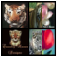
(a) target attribute: tulip

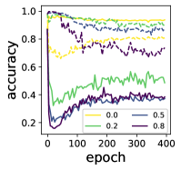
(b) — tulip;  - - tractor

(c) target attribute: tractor

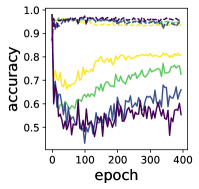
(d) — tractor;  - - tulip

Figure B.5: (a) displays the modified dataset with four types of images: tiger (top left) and half-tiger-half-tulip (top right) belong to class 1, while leopard (bottom left) and half-leopard-half-tulip (bottom right) belong to class 2. The model is trained to distinguish between class 1 and class 2. Since ‘tulip’ is class-irrelevant in this dataset, we expect finetuning to cause the model to forget ‘tulip’. The fraction of half-half images in the dataset is roughly $\alpha$ due to its construction. (b) shows the accuracy on ‘tulip’ (solid line) and ‘tractor’ (dashed line) against training epochs, with colors representing values of $\alpha$. We observe that when $\alpha=0$ (i.e., without the half-tulip images), the model does not forget ‘tulip’ even after 400 epochs of training. As we increase $\alpha$, the accuracy on ‘tulip’ drops significantly and eventually reaches random guess accuracy, while the accuracy on ‘tractor’ (which is not present in the training set) remains relatively high. To demonstrate that this phenomenon is not specific to the selection of images, we perform a similar experiment with ‘tractor’ as the target feature. (c) displays the example images in the constructed dataset, and (d) demonstrates a similar pattern. For each $\alpha$, we report the average of 5 runs with different random seeds.

Our experiment on a semi-synthetic dataset confirms the observations made through theoretical analysis in Section 4.3.2, showing that they hold for real neural networks. Specifically, we demonstrate that if a pretrained model learns an attribute, finetuning the model on a dataset without this attribute cannot fully remove it. However, when finetuning the model on a dataset where this attribute occurs uniformly, the attribute can be effectively removed.

We pretrained a ResNet18 on four classes from CIFAR100: ‘tiger’, ‘tulip’, ‘leopard’, and ‘tractor’, with the goal of predicting whether an image belonged to [‘tiger’, ‘tulip’] or [‘leopard’, ‘tractor’]. After pretraining, the model has learned to classify all four types of images. We then define a downstream task where the goal is to classify ‘tiger’ and ‘leopard’, while forgetting either ‘tulip’ or ‘tractor’ (which we call the target attribute). We construct the following modified dataset for finetuning: we start with all examples from ‘tiger’ and ‘leopard’; for each example, we remove the right half with probability $\alpha$ and replace it with the right half of a random example with the target attribute (i.e., an example from ‘tulip’ or ‘tractor’). See Figures 5(a) and 5(c) for an illustration of the constructed dataset. Note that $\alpha=0$ recovers the dataset with only images of ‘tiger’ and ‘leopard’.

We first let ‘tulip’ be the target attribute that we want to remove, and Figure 5(b) demonstrates that when $\alpha=0$, the model retains the ability to classify ‘tulip’ with an accuracy of approximately 80% even after 400 epochs of training. However, when we let $\alpha>0$, we observe that increasing $\alpha$ leads to faster and more effective forgetting of ‘tulip’, compared to ‘tractor’, which is not shown in the finetuning set. We also demonstrate that this phenomenon is not an artifact of the selection of classes by letting ‘tractor’ be the target feature and showing the same pattern in Figure 5(d).

Appendix C Details of Experiments on Standard Benchmarks

All experiments are implemented using PyTorch. We use eight Nvidia A40 to run the experiments.

C.1 Datasets

In WaterBirds the labels are $landbird$ and $waterbird$. The attributes are the image backgrounds, which are $land$ and $water$. In the training set, the size of four groups $(land,landbird)$, $(water,landbird)$, $(land,waterbird)$ and $(water,waterbird)$ are 3498, 184, 56 and 1057, respectively. In CelebA the labels are $blond$ and $non~{}blond$. The minority group in the training set is $(male,blond)$. Civilcomments is a dataset of online comments with labels ‘toxic’ and ‘non-toxic’. The attributes are indicator of whether the following 8 demographic identities are mentioned in the comment: male, female, LGBTQ, Christian, Muslim, other religion, Black, and White. We follow [Koh et al., 2021, Liu et al., 2021] and consider the 16 potentially overlapping groups: $(identity,toxic)$ and $(identity,not~{}toxic)$ for all 8 identities. We also consider the 4 non-overlapping groups $(black,not~{}toxic)$, $(not~{}black,not~{}toxic)$, $(black,toxic)$ and $(not~{}black,toxic)$ in Section 5.1.2, following [Koh et al., 2021].

C.2 Baselines

Empirical risk minimization (ERM) is the standard training procedure which directly minimizes the training loss. GroupDRO [Sagawa et al., 2019] is an oracle approach which requires the group information of all training data and use it to upweight worst-group examples. SUBG [Idrissi et al., 2022] applies ERM to a randomly selected subset of the data, where the groups are equally represented. CVaR DRO [Levy et al., 2020] seeks to minimize error over all groups above a certain size. JTT [Liu et al., 2021] detects missclassified examples after training and retrains the model with those examples upweighted. In CnC [Zhang et al., 2022], group information is inferred through either examining misclassification or clustering, and contrastive learning is utilized to learn similar representations for samples belonging to the same class. SSA [Nam et al., 2022] is a semi-supervised learning apporach which utilizes the group information from the validation set to train a group label predictor. It trains a group label predictor to infer group information on the training set, and then applies GroupDRO based on the inferred group information.

C.3 Training Details

Pretraining

We use ERM to pretrain the models, allowing them to learn the spurious correlations. For WaterBirds, we pretrain a ResNet-50 for 100 epochs with weight decay 0.001, batchsize 32, and learning rate 0.001.The pretrained model has a worst-group accuracy of 74%. For CelebA, we pretrain a ResNet-50 for 50 epochs with weight decay 0.0001, batchsize 128, and learning rate 0.001. The pretrained model has a worst-group accuracy of 42%. For CivilComments, we pretrain a Bert for 5 epochs, with weight decay 0.01, batchsize 16 and learning rate 0.00001. The pretrained model has a worst-group accuracy of 56.34%. Note that the accuracies here are lower than the numbers reported in Table 1 because we directly use the model at the last epoch as the pretrained model, whereas the numbers in the table are from other papers that employed early stopping based on validation for ERM.

$\mathcal{D}_{\text{FT}}$ and $\mathcal{D}_{\text{BA}}$

When $\mathcal{D}_{\text{FT}}$ and $\mathcal{D}_{\text{BA}}$ are drawn from the validation data, the details have already been described in Section 5.1. When they are drawn from the training data, $\mathcal{D}_{\text{BA}}$ still consists of $l$ examples randomly drawn from each group. The details of $\mathcal{D}_{\text{FT}}$ vary depending on the dataset, as the size of the training set differs significantly across datasets. For WaterBirds, we randomly upsample examples from the smaller class to match the size of the larger class. On CelebA, since the training set is very large, we only sample 25000 examples from each class (with replacement for the smaller class) to reduce computation cost. On CivilComments, we randomly sample 5000 examples from each class when $l\neq$ max, and 100000 examples from each class when $l=$max since the maximal $l$ is already large.

Implementation

On WaterBirds and CelebA, we implement Dispel within the framework of DFR and follow their procedure: we use logistic regression with $l_{1}$ regularization to train a linear model on representations generated using Dispel, and we repeat the training 10 times on different random subsets of the data, averaging the weights of the learned models. For CivilComments, we only train a single linear model using stochastic gradient descent (SGD) and perform early stopping based on worst-group accuracy on the validation set, following the same procedure as in [Sagawa et al., 2019, Liu et al., 2021].

Hyperparameters

(1) When $\mathcal{D}_{\text{FT}}$ and $\mathcal{D}_{\text{BA}}$ are drawn from validation data. For WaterBirds and CelebA, following [Kirichenko et al., 2022], we tune the inverse regularization strength parameter for $l_{1}$ regularization in the range $\{1,0.7,0.3,0.1,0.07,0.03,0.01\}$. Additionally, we set $\alpha=1$ and tune the scale parameter $s$ for $l=$max on both datasets, using the range $\{1,0.95,0.9,0.85,0.8,0.75,0.7\}$. For $l=10$, we tune $s$ using the range $\{0.5,0.45,0.4,0.35,0.3,0.25,0.2,0.15,0.1\}$ on WaterBirds and $\{0.8,0.75,0.7,0.65,0.6,0.55,0.5,0.45,0.4\}$ on CelebA. The ranges are determined based on the results of a single trial with a fixed random seed. For CivilComments, since we use SGD to train the linear layer, we set learning rate to 0.01 and do not use weight decay. For both $l$=max and $l=20$, We tune tune $\alpha$ in the range $\{1.0,0.8,0.6,0.4,0.2\}$ and $s$ in the range $\{1.0,0.99,0.97,0.95,0.9\}$. Our results can potentially be improved further by additionally tuning learning rate and weight decay, as in previous works. (2) When $\mathcal{D}_{\text{FT}}$ and $\mathcal{D}_{\text{BA}}$ are drawn from training data. the ranges for $\alpha$ and $s$ are the same except: on WaterBirds with $l=10$ we additionally include the range $\{0.7,0.65,0.6,0.55\}$ for $s$; on CivilComments we use the range $\{0.1,0.2,0.3,0.5,0.7,0.9,1.0\}$ for $s$. Moreover, on WaterBirds and CelebA, following [Kirichenko et al., 2022], we also tune the class weight when training data are used. We set the weight for one of the classes to 1 and consider the weights for the other class in range $\{1,2,3,10,100,300,1000\}$; we then switch the classes and repeat the procedure.

Other Details in Table 1

(*) shows results obtained by running the code provided by [Kirichenko et al., 2022] and taking the average of 10 runs, which may slightly differ from the numbers reported in [Kirichenko et al., 2022]. Numbers with ($\diamondsuit$) shows the highest worst-group performance of the two DFR implementations in Table D.4. For Dispel and $\text{DFR}^{\text{Val}}_{\text{Tr}}$we report the average of 10 runs on Waterbirds and CelebA, and 5 runs on CivilComments.

Appendix D Additional Experimental Results for Section 5

D.1 Details of Results for DFR on CivilComments

In [Kirichenko et al., 2022], DFR was implemented using logistic regression with $l_{1}$ regularization and averaging weights from multiple retraining. However, since [Kirichenko et al., 2022] did not provide code for CivilComments and some implementation details are unknown, and only the result for $l=$max was reported, we do not have the numbers for other values of $l$ on CivilComments. Additionally, it should be noted that on CivilComments, we use SGD with early stopping for Dispel. To ensure a fair comparison, we implement DFR with SGD and early stopping (which is equivalent to Dispel with $\alpha$ and $s$ both fixed to 1), and then compare our method Dispel with the highest number of two implementations of DFR whenever both numbers are available. The results for two implementations of DFR are presented in Table D.4. We observe that our implementation (SGD with early stopping) of DFR actually performs better than the original one, with the margin especially significant for $\text{DFR}^{\text{Tr}}_{\text{Tr}}$. Despite this, our proposed method Dispel outperforms both versions of DFR, as shown in Table 1.

Table D.4: Comparison between two implementations of DFR. The SGD based implementation performs better than the implementation in [Kirichenko et al., 2022].

	Implementation	Wg (%)	Avg (%)
$\text{DFR}^{\text{Val}}_{\text{Tr}}$   $l=$max	SGD w/ early stopping	$70.1_{\pm 1.5}$	$89.1_{\pm 0.9}$
	$l_{1}$ LogReg w/ multi-retraining & averaging	$70.1_{\pm 0.8}$	$87.2_{\pm 0.3}$
$\text{DFR}^{\text{Val}}_{\text{Tr}}$   $l=20$	SGD w/ early stopping	$68.5_{\pm 3.0}$	$89.0_{\pm 1.0}$
	$l_{1}$ LogReg w/ multi-retraining & averaging	-	-
$\text{DFR}^{\text{Tr}}_{\text{Tr}}$   $l=$max	SGD w/ early stopping	$65.0_{\pm 2.2}$	$90.8_{\pm 0.3}$
	$l_{1}$ LogReg w/ multi-retraining & averaging	$58.0_{\pm 1.3}$	$92.0_{\pm 0.1}$
$\text{DFR}^{\text{Tr}}_{\text{Tr}}$   $l=20$	SGD w/ early stopping	$65.6_{\pm 5.4}$	$89.5_{\pm 1.3}$
	$l_{1}$ LogReg w/ multi-retraining & averaging	-	-

D.2 When $\mathcal{D}_{\text{FT}}$ and $\mathcal{D}_{\text{BA}}$ are Drawn from Training Data

Results on CivilComments with various values of $l$ are presented in Table D.6.

Figure D.6: Dispel achieves significantly better performance compared to $\text{DFR}^{\text{Tr}}_{\text{Tr}}$on CivilComments when $\mathcal{D}_{\text{BA}}$ is composed of training data.

Method	$l$	Wg (%)	Avg (%)
Dispel	5	$70.5_{\pm 1.7}$	$90.2_{\pm 0.3}$
	20	$71.2_{\pm 1.6}$	$89.9_{\pm 0.3}$
	100	$70.8_{\pm 1.3}$	$90.2_{\pm 0.3}$
	max	$70.1_{\pm 0.8}$	$90.1_{\pm 0.2}$
$\text{DFR}^{\text{Tr}}_{\text{Tr}}$ ($l_{1}$ SGD w/ early-stopping	5	$61.9_{\pm 1.6}$	$91.4_{\pm 0.5}$
	20	$65.6_{\pm 5.4}$	$89.5_{\pm 1.3}$
	100	$67.2_{\pm 3.1}$	$89.8_{\pm 0.4}$
	max	$65.0_{\pm 2.2}$	$90.8_{\pm 0.3}$
$\text{DFR}^{\text{Tr}}_{\text{Tr}}$ ($l_{1}$ LogReg w/ multi-retraining & averaging)	max	$58.0_{\pm 1.3}$	$92.0_{\pm 0.1}$

D.3 Applying Dispel to the Inputs and Finetuning the Entire Network

Table D.5: Results for finetuning the entire network on CelebA with $\mathcal{D}_{\text{FT}}$ and $\mathcal{D}_{\text{BA}}$ drawn from the training data.

$l$	Wg (%)	Avg (%)
10	$83.2_{\pm 1.4}$ %	$89.3_{\pm 0.9}$%
25	$83.3_{\pm 2.5}$%	$88.4_{\pm 0.6}$%
50	$86.3_{\pm 1.7}$%	$90.4_{\pm 0.3}$%
100	$87.6_{\pm 1.4}$ %	$89.9_{\pm 0.3}$%

Table D.6: Results for finetuning the entire network on CelebA with $\mathcal{D}_{\text{FT}}$ and $\mathcal{D}_{\text{BA}}$ drawn from the validation data.

$l$	Wg (%)	Avg (%)
50	$86.1_{\pm 1.0}$%	$95.2_{\pm 0.7}$%

Table D.7: Results for finetuning the entire network on WaterBirds with $\mathcal{D}_{\text{FT}}$ and $\mathcal{D}_{\text{BA}}$ drawn from the training data.

$l$	Wg (%)	Avg (%)
10	$79.5_{\pm 1.1}$%	$96.0_{\pm 0.3}$%
50	$86.1_{\pm 1.0}$%	$95.2_{\pm 0.7}$%
max	$86.7_{\pm 1.5}$%	$95.8_{\pm 0.2}$%

Table D.8: Results for finetuning the entire network on WaterBirds with $\mathcal{D}_{\text{FT}}$ and $\mathcal{D}_{\text{BA}}$ drawn from the validation data.

$l$	Wg (%)	Avg (%)
10	$89.3_{\pm 1.4}$%	$93.8_{\pm 1.2}$%
max	$90.6_{\pm 0.5}$%	$93.6_{\pm 1.4}$%

Instead of applying Dispel to the representations and retraining only the last layer, an alternative approach is to apply Dispel directly to the original inputs of the data and fine-tune the entire network. Except on on CelebA with $\mathcal{D}_{\text{FT}}$ and $\mathcal{D}_{\text{BA}}$ drawn from the training data (Table D.5), this approach does lead to better performance. Other results are in Tables D.6, D.7 and D.8.

D.4 Effects of $\alpha$ and $s$ on CivilComments

Figure D.7 shows the worst-group accuracy achieved under different combinations of $\alpha$ and $s$ when $\mathcal{D}_{\text{FT}}$ and $\mathcal{D}_{\text{BA}}$ are drawn from the training data. The result is for a single trial with fixed random seed. Note that when $s=0$ only $\mathcal{D}_{\text{FT}}$ is used and when $\alpha=1,s=1$ only $\mathcal{D}_{\text{BA}}$ is used. We see that the best performance is achieved at intermediate $\alpha$ and $s$, which highlights the benefit of combining the two datasets $\mathcal{D}_{\text{FT}}$ and $\mathcal{D}_{\text{BA}}$.

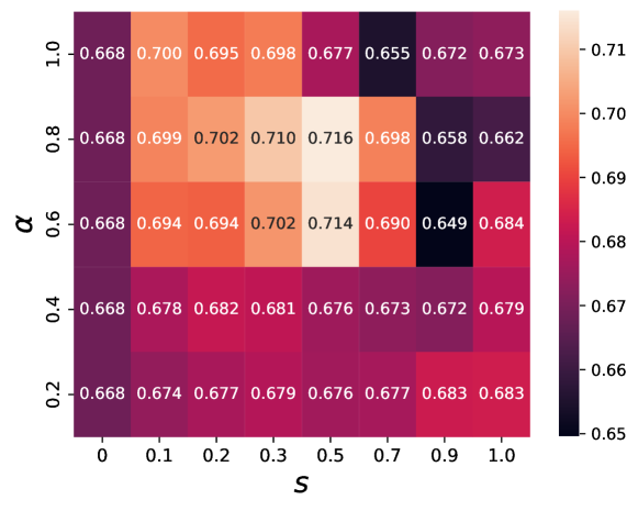
Figure D.7: Worst-group accuracy (indicated by colors and annotations) achieved under different combinations of $\alpha$ and $s$ on CivilComments. The result is for a single trial with fixed random seed.

D.5 Experiments on Modified CivilComments with Severe Bias

For Dispel, we let $\mathcal{D}_{\text{BA}}$ consist of 100 examples randomly selected from group $(black,toxic)$ in the training set, and let $\mathcal{D}_{\text{FT}}$ be the entire training set. As for the DFR, we retrain the last layer of the model using SGD on 3111 examples from each of the three available groups where 3111 is size of the smallest group in the trainig data.

Appendix E Details of Experiments on ImageNet

All experiments are implemented using PyTorch. We use eight Nvidia A40 to run the experiments.

E.1 Adversarial Finetuning of the Entire Network is Necessary for Preserving Adversarial Performance

In Table E.9, we present a comparison of adversarial accuracies of models trained in different ways. The models are evaluated using the ‘robustness’ library [Engstrom et al., 2019]. For adversarial training and evaluation, we consider the threat model as an $l_{2}$ ball of radius 3. The last two rows in the table correspond to the models trained using Dispel, with the goal of eliminating $lighter$-$flame$ and $rhodesian~{}ridgeback$-$colllar$ correlations, respectively (detailes will be described later). We observe that simply retraining the last layer would cause a significant drop in adversarial accuracy, while finetuning the entire network adversarially preserves the accuracy. For this reason, in our experiments in Section 5.2, we apply Dispel to the inputs instead of the representations.

Table E.9: Adversarial finetuning of the entire network preserves adversarial accuracy, while retraining only the last layer results in a significant drop in accuracy. We also provide the adversarial accuracy of a normally pretrained model for reference (with the number taken from [Engstrom et al., 2019]).

	$l_{2}$-robust accuracy ($\epsilon=3$)
Pretrained (normally)	0.13%
Pretrained (adversarially with $\epsilon=3$)	35.16%
Last layer retraining (200 examples per class)	23.50%
Last layer retraining (all data)	24.984%
Adversarial finetuning ($lighter$-$flame$)	35.54%
Adversarial finetuning ($ridgeback$-$collar$)	35.37%

E.2 $\mathcal{D}_{\text{FT}}$ and $\mathcal{D}_{\text{BA}}$

We use the feature extractor provided by Barlow [Singla et al., 2021] (described in Section E.4) to automatically identify 432 images of lighters that are likely to have a flame. We then remove these images from the full ImageNet dataset and sample only 200 examples from each class to construct $\mathcal{D}_{\text{FT}}$ for finetuning, which is approximately a no-spurious dataset with few images of lights with flames. We would like to emphasize that this does not favor our method in any way. Instead, it enables us to compare between Dispel and finetuning on a no-spurious dataset (i.e., $\mathcal{D}_{\text{FT}}$ only).

We create $\mathcal{D}_{\text{BA}}$ by randomly sampling 180 of the aforementioned 432 images, with almost all of the images in $\mathcal{D}_{\text{BA}}$ belonging to the $(flame,lighter)$ group.

For the experiment where we aim at removing the spurious correlation between attribute $collar$ and class $rhodesian~{}ridgeback$, we first use the feature extractor to automatically identify 24 images in class $rhodesian~{}ridgeback$ that are most likely to have collar. Then we remove them from the training dataset and sample 200 examples from each each class to construct $\mathcal{D}_{\text{FT}}$. We create $\mathcal{D}_{\text{BA}}$ using the aforementioned 24 images, all of which belong to group $(collar,rhodesian~{}ridgeback)$

E.3 Training Details

We use the same pretrained model as [Singla et al., 2021] and adopt the same finetuning algorithm as used for pretraining but with a smaller learning rate: adversarial training where the threat model is an $l_{2}$ ball of radius 3 and the learning rate is set to 0.01. Following [Singla et al., 2021], we use the ImageNet training set to calculate group performance, as opposed to the validation set, due to the significantly larger number of images per class (1300 compared to 50 in the validation set). For Dispel, we set $\alpha=0.4,s=0.1$ for $flame-lighter$, and $\alpha=0.4,s=0.05$ for $collar-rhodesian~{}ridgeback$. For DFR, we let the training set consist of 200 examples from each of the groups. Note that for $flame-lighter$, the groups are $(flame,lighter)$, $(no~{}flame,lighter)$ and $(no~{}flame,y)$ for $y\neq lighter$. Similarly, for $collar-rhodesian~{}ridgeback$ the groups are $(collar,rhodesian~{}ridgeback)$, $(no~{}collar,rhodesian~{}ridgeback)$ and $(no~{}collar,y)$ for $y\neq rhodesian~{}ridgeback$.

E.4 How Barlow Works

Barlow first finds the neuron $u$ in the penultimate layer whose absence is most responsible for wrong predictions in the given class, then displays three rows of images telling us what concept $u$ represents. For example, Figure E.8 is the result for the pretrained model. The first row displays images that maximally activate this neuron $u$. The second row displays regions within these images that maximally activate $u$. The third row displays a feature attack that amplifies the inputs that maximally activate neuron $u$. Overall, Figure E.8 tells us the absence of flame lets the pretrained model make wrong predictions given images of lighter.

E.5 Visualization of the Cause of Wrong Predictions for Pretrained Models

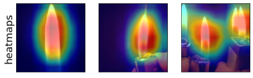
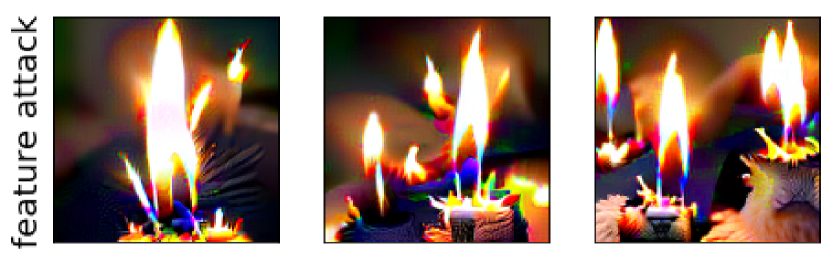
Figure E.8: Barlow visualization on class $lighter$ for the adversarially pretrained model.

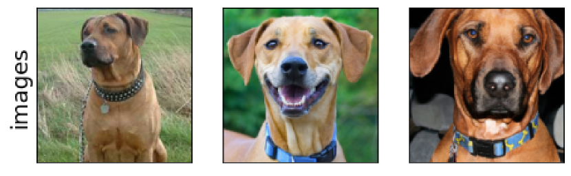
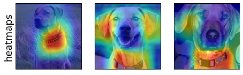
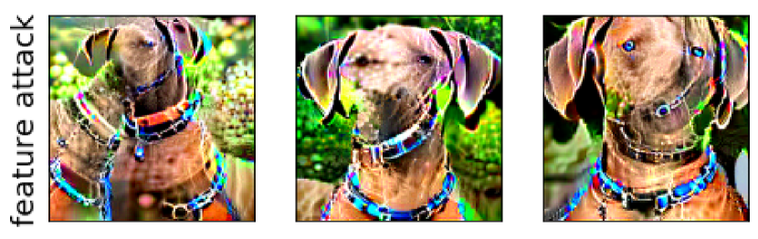
Figure E.9: Barlow visualization on class $rhodesian~{}ridgeback$ for the adversarially pretrained model.

Figure E.8 illustrates that the absence of attributes resembling flames is the primary cause of wrong predictions in the class $lighter$. Similarly, Figure E.8 illustrates that attributes resembling collars are the primary cause of wrong predictions in the class $rhodesian~{}ridgeback$.

References

- Hendrycks et al. (2019) Dan Hendrycks, Kimin Lee, and Mantas Mazeika. Using pre-training can improve model robustness and uncertainty. In International Conference on Machine Learning, pages 2712–2721. PMLR, 2019.
- He et al. (2017) Kaiming He, Georgia Gkioxari, Piotr Dollár, and Ross Girshick. Mask r-cnn. In Proceedings of the IEEE international conference on computer vision, pages 2961–2969, 2017.
- Liu et al. (2019) Yinhan Liu, Myle Ott, Naman Goyal, Jingfei Du, Mandar Joshi, Danqi Chen, Omer Levy, Mike Lewis, Luke Zettlemoyer, and Veselin Stoyanov. Roberta: A robustly optimized bert pretraining approach. arXiv preprint arXiv:1907.11692, 2019.
- Gururangan et al. (2018) Suchin Gururangan, Swabha Swayamdipta, Omer Levy, Roy Schwartz, Samuel R Bowman, and Noah A Smith. Annotation artifacts in natural language inference data. arXiv preprint arXiv:1803.02324, 2018.
- McCoy et al. (2019) R Thomas McCoy, Ellie Pavlick, and Tal Linzen. Right for the wrong reasons: Diagnosing syntactic heuristics in natural language inference. arXiv preprint arXiv:1902.01007, 2019.
- Salman et al. (2022) Hadi Salman, Saachi Jain, Andrew Ilyas, Logan Engstrom, Eric Wong, and Aleksander Madry. When does bias transfer in transfer learning? arXiv preprint arXiv:2207.02842, 2022.
- Liu et al. (2021) Evan Z Liu, Behzad Haghgoo, Annie S Chen, Aditi Raghunathan, Pang Wei Koh, Shiori Sagawa, Percy Liang, and Chelsea Finn. Just train twice: Improving group robustness without training group information. In International Conference on Machine Learning, pages 6781–6792. PMLR, 2021.
- Sagawa et al. (2019) Shiori Sagawa, Pang Wei Koh, Tatsunori B Hashimoto, and Percy Liang. Distributionally robust neural networks. In International Conference on Learning Representations, 2019.
- Creager et al. (2021) Elliot Creager, Jörn-Henrik Jacobsen, and Richard Zemel. Environment inference for invariant learning. In International Conference on Machine Learning, pages 2189–2200. PMLR, 2021.
- Han et al. (2022) Zongbo Han, Zhipeng Liang, Fan Yang, Liu Liu, Lanqing Li, Yatao Bian, Peilin Zhao, Bingzhe Wu, Changqing Zhang, and Jianhua Yao. Umix: Improving importance weighting for subpopulation shift via uncertainty-aware mixup. arXiv preprint arXiv:2209.08928, 2022.
- Zhang et al. (2022) Michael Zhang, Nimit S Sohoni, Hongyang R Zhang, Chelsea Finn, and Christopher Ré. Correct-n-contrast: A contrastive approach for improving robustness to spurious correlations. arXiv preprint arXiv:2203.01517, 2022.
- Kirichenko et al. (2022) Polina Kirichenko, Pavel Izmailov, and Andrew Gordon Wilson. Last layer re-training is sufficient for robustness to spurious correlations. arXiv preprint arXiv:2204.02937, 2022.
- Borkan et al. (2019) Daniel Borkan, Lucas Dixon, Jeffrey Sorensen, Nithum Thain, and Lucy Vasserman. Nuanced metrics for measuring unintended bias with real data for text classification. In Companion proceedings of the 2019 world wide web conference, pages 491–500, 2019.
- Liu et al. (2015) Ziwei Liu, Ping Luo, Xiaogang Wang, and Xiaoou Tang. Deep learning face attributes in the wild. In Proceedings of the IEEE international conference on computer vision, pages 3730–3738, 2015.
- Singla et al. (2021) Sahil Singla, Besmira Nushi, Shital Shah, Ece Kamar, and Eric Horvitz. Understanding failures of deep networks via robust feature extraction. In Proceedings of the IEEE/CVF Conference on Computer Vision and Pattern Recognition, pages 12853–12862, 2021.
- Madry et al. (2017) Aleksander Madry, Aleksandar Makelov, Ludwig Schmidt, Dimitris Tsipras, and Adrian Vladu. Towards deep learning models resistant to adversarial attacks. arXiv preprint arXiv:1706.06083, 2017.
- Deng et al. (2009) Jia Deng, Wei Dong, Richard Socher, Li-Jia Li, Kai Li, and Li Fei-Fei. Imagenet: A large-scale hierarchical image database. In 2009 IEEE conference on computer vision and pattern recognition, pages 248–255. Ieee, 2009.
- Cui et al. (2019) Yin Cui, Menglin Jia, Tsung-Yi Lin, Yang Song, and Serge Belongie. Class-balanced loss based on effective number of samples. In Proceedings of the IEEE/CVF conference on computer vision and pattern recognition, pages 9268–9277, 2019.
- He and Garcia (2009) Haibo He and Edwardo A Garcia. Learning from imbalanced data. IEEE Transactions on knowledge and data engineering, 21(9):1263–1284, 2009.
- Byrd and Lipton (2019) Jonathon Byrd and Zachary Lipton. What is the effect of importance weighting in deep learning? In International Conference on Machine Learning, pages 872–881. PMLR, 2019.
- Shimodaira (2000) Hidetoshi Shimodaira. Improving predictive inference under covariate shift by weighting the log-likelihood function. Journal of statistical planning and inference, 90(2):227–244, 2000.
- Arjovsky and Bottou (2017) Martin Arjovsky and Léon Bottou. Towards principled methods for training generative adversarial networks. arXiv preprint arXiv:1701.04862, 2017.
- Nam et al. (2020) Junhyun Nam, Hyuntak Cha, Sungsoo Ahn, Jaeho Lee, and Jinwoo Shin. Learning from failure: De-biasing classifier from biased classifier. Advances in Neural Information Processing Systems, 33:20673–20684, 2020.
- Nam et al. (2022) Junhyun Nam, Jaehyung Kim, Jaeho Lee, and Jinwoo Shin. Spread spurious attribute: Improving worst-group accuracy with spurious attribute estimation. arXiv preprint arXiv:2204.02070, 2022.
- He et al. (2016) Kaiming He, Xiangyu Zhang, Shaoqing Ren, and Jian Sun. Deep residual learning for image recognition. In Proceedings of the IEEE conference on computer vision and pattern recognition, pages 770–778, 2016.
- Devlin et al. (2018) Jacob Devlin, Ming-Wei Chang, Kenton Lee, and Kristina Toutanova. Bert: Pre-training of deep bidirectional transformers for language understanding. arXiv preprint arXiv:1810.04805, 2018.
- Koh et al. (2021) Pang Wei Koh, Shiori Sagawa, Henrik Marklund, Sang Michael Xie, Marvin Zhang, Akshay Balsubramani, Weihua Hu, Michihiro Yasunaga, Richard Lanas Phillips, Irena Gao, et al. Wilds: A benchmark of in-the-wild distribution shifts. In International Conference on Machine Learning, pages 5637–5664. PMLR, 2021.
- Levy et al. (2020) Daniel Levy, Yair Carmon, John C Duchi, and Aaron Sidford. Large-scale methods for distributionally robust optimization. Advances in Neural Information Processing Systems, 33:8847–8860, 2020.
- Idrissi et al. (2022) Badr Youbi Idrissi, Martin Arjovsky, Mohammad Pezeshki, and David Lopez-Paz. Simple data balancing achieves competitive worst-group-accuracy. In Conference on Causal Learning and Reasoning, pages 336–351. PMLR, 2022.
- Engstrom et al. (2019) Logan Engstrom, Andrew Ilyas, Hadi Salman, Shibani Santurkar, and Dimitris Tsipras. Robustness (python library), 2019. URL https://github.com/MadryLab/robustness.