Confidence sets for Causal Orderings

Abstract.

Causal discovery procedures aim to deduce causal relationships among variables in a multivariate dataset. While various methods have been proposed for estimating a single causal model or a single equivalence class of models, less attention has been given to quantifying uncertainty in causal discovery in terms of confidence statements. The primary challenge in causal discovery is determining a causal ordering among the variables. Our research offers a framework for constructing confidence sets of causal orderings that the data do not rule out. Our methodology applies to structural equation models and is based on a residual bootstrap procedure to test the goodness-of-fit of causal orderings. We demonstrate the asymptotic validity of the confidence set constructed using this goodness-of-fit test and explain how the confidence set may be used to form sub/supersets of ancestral relationships as well as confidence intervals for causal effects that incorporate model uncertainty.

1. Introduction

Inferring causal relations as opposed to mere associations is a problem that is not only of intrinsic scientific interest but also helps predict how an observed system might change under intervention (Peters et al.,, 2017). When randomized controlled trials are infeasible, methods for causal discovery—the problem of estimating a causal model from observational data—become valuable tools for hypothesis generation and acceleration of scientific progress. Examples of applications include systems biology (Sachs et al.,, 2005), neuroscience (Shen et al.,, 2020), and climate modeling (Nowack et al.,, 2020).

Causal models may be represented as a directed acyclic graph (DAG), and—leveraging this representation—causal discovery can be cast as recovering the appropriate DAG. The first step in causal discovery is identification: determining appropriate assumptions under which the causal model can be recovered from population information; see, e.g., Shimizu et al., (2006); Loh and Bühlmann, (2014); Peters et al., (2014). The next step is providing a method to estimate the causal graph from data; see, e.g., Bühlmann et al., (2014); Chen et al., (2019); Wang and Drton, 2020b . Once an estimation procedure is established, it is natural to question the estimation uncertainty. Uncertainty quantification and the ability to test identifying assumptions are essential for trustworthy estimation of causal graphs and help to determine whether key modeling assumptions are appropriate. Nonetheless, the literature on frequentist causal discovery, with a few exceptions (e.g., Strobl et al.,, 2019), only outputs a point estimate in the form of a DAG or single equivalence class.

Given a causal ordering of the variables, causal discovery reduces to variable selection in a sequence of regressions. Thus, the key difficulty lies in inferring the causal ordering; this motivates the issue we address in this paper: developing a procedure that provides a confidence set for causal orderings.

1.1. Setup

We represent a causal model for the random vector $Y=(Y_{1},\dots,Y_{p})$ with a DAG $G=(V,E)$, where each node $v$ in the vertex set $V=[p]$ indexes a random variable $Y_{v}$. An edge $u\rightarrow v\in E$ indicates that $Y_{u}$ has a direct causal effect on $Y_{v}$, and we say that $u$ is a parent of its child $v$. If there exists a directed path in $G$ from $u$ to $v$, then $u$ is an ancestor of its descendant $v$ . We denote the sets of parents, children, ancestors, and descendants of node $v$ by ${\rm pa}(v)$, ${\rm ch}(v)$, ${\rm an}(v)$, and ${\rm de}(v)$, respectively. The models we consider take the form of a recursive structural equation model (SEM) with additive noise:

(1.1) $$\small Y_{v}=f_{v}\left((Y_{u})_{u\in{\rm pa}(v)}\right)+\varepsilon_{v},\qquad v\in V,$$

where the $f_{v}$ are unknown and the errors $\{\varepsilon_{v}\}_{v=1}^{p}$ are mean zero and mutually independent.

In a fully general SEM, the DAG may only be identified from observational data up to a Markov equivalence class—a collection of graphs that imply the same set of conditional independence relations (Spirtes et al.,, 2000). As the different graphs in the equivalence class may have contradicting causal interpretations, it is also of interest to work with restricted SEMs in which the DAG itself becomes identifiable (Maathuis et al.,, 2019, Chap. 18.6.3). Specifically, for the model in (1.1), the DAG becomes identifiable when $f_{v}$ are non-linear or the errors $\varepsilon_{v}$ non-Gaussian. In contrast, the linear Gaussian case, also allowed under (1.1), features the same Markov equivalence classes as the general nonparametric model.

We focus on a causal ordering for the variables in the model given by DAG $G$; i.e., a total ordering of $V$ where variables that appear later have no causal effect on earlier variables. We may identify each possible ordering with a permutation $\theta:V\to V$, where $\theta$ yields a causal ordering for $G$ if and only if $\theta(u)<\theta(v)$ implies that $v\not\in{\rm an}(u)$. In general, a causal ordering is not unique, and, letting $\mathcal{S}_{V}$ be the set of all permutations of $V$, we denote the set of all causal orderings $\Theta(G)=\left\{\theta\in\mathcal{S}_{V}\,:\,\theta(u)<\theta(v)\text{ only if }v\not\in{\rm an}(u)\right\}.$

1.2. Contribution

Let $\mathbf{Y}$ be a sample drawn from the SEM in (1.1), and let $\alpha\in(0,1)$. We propose a procedure that constructs a $1-\alpha$ confidence set of causal orderings, $\hat{\Theta}(\mathbf{Y},\alpha)$, where $\hat{\Theta}(\mathbf{Y},\alpha)\subseteq\mathcal{S}_{V}$. Specifically, our procedure inverts a goodness-of-fit test for a causal ordering and returns the set of all orderings that are not rejected by the test. Thus, for any $\theta\in\Theta(G)$:

(1.2) $$\small\lim_{n\rightarrow\infty}P\left(\theta\in\hat{\Theta}(\mathbf{Y},\alpha)\right)\geq 1-\alpha.$$

It follows that if $G$ has a unique causal ordering (i.e., $|\Theta(G)|=1$), then $\hat{\Theta}(\mathbf{Y},\alpha)$ contains that causal ordering with asymptotic probability at least $1-\alpha$. If $|\Theta(G)|>1$, then our procedure still infers a valid causal ordering—i.e., $\Theta(G)\cap\hat{\Theta}(\mathbf{Y},\alpha)\neq\emptyset$—with asymptotic probability at least $1-\alpha$.

The confidence set $\hat{\Theta}(\mathbf{Y},\alpha)$ provides a set of orderings that are not excluded by the data. Different elements of $\hat{\Theta}(\mathbf{Y},\alpha)$ suggest different causal orderings which may, but do not have to, lead to different causal conclusions; we elaborate on this point in Section 4.3. The set $\hat{\Theta}(\mathbf{Y},\alpha)$ being large cautions the analyst against overconfidence in a specific estimated ordering. In contrast, if $\hat{\Theta}(\mathbf{Y},\alpha)$ is small, few causal orderings are compatible with the data under the considered model class. This latter aspect is crucial because $\hat{\Theta}(\mathbf{Y},\alpha)$ may also be empty, indicating that the model class does not capture the data-generating process.

Furthermore, $\hat{\Theta}(\mathbf{Y},\alpha)$ can be post-processed to form other useful objects. Most notably, similar to the problem studied by Strieder et al., (2021), we may form confidence intervals for causal effects that also incorporate model uncertainty. In addition, $\hat{\Theta}(\mathbf{Y},\alpha)$ yields a sub/superset of the true ancestral relationships with some user-defined probability.

Our framework takes a straightforward approach based on goodness-of-fit tests. However, realizing this idea presents significant challenges, and we construct our procedure with careful attention to both statistical and computational aspects. Specifically, our methodology is built using computationally attractive tests for regression models with asymptotic validity under $p=o(n)$, where $p$ is the number of variables and $n$ is the sample size. Computationally, we devise the statistical decisions so that we can use a branch-and-bound type procedure to handle problems at a moderate but challenging scale. Despite prioritizing computational tractability, the procedure is asymptotically valid when allowing $p$ to grow with $n$, and we establish the asymptotic validity of the confidence set when $p^{4}=o(n)$.

To motivate $\hat{\Theta}(\mathbf{Y},\alpha)$ as an object of interest, we preview the analysis in Section 6.3 of daily stock returns for 12 industry portfolios. DirectLiNGAM (Shimizu et al., 2011a, ) gives a point estimate of the causal ordering where the Utilities industry is first and causally precedes the other 11 industries. The set $\hat{\Theta}(\mathbf{Y},.05)$ contains approximately $1/15,000$ of the $12!$ possible total orderings, and indeed Utilities is first in every ordering in the confidence set. Nonetheless, many orderings in $\hat{\Theta}(\mathbf{Y},\alpha=.05)$—i.e., those not rejected by the data—have other causal implications which differ from the point estimate. As shown in Section 6.3, the point estimate is quite far from the Fréchet mean of $\hat{\Theta}(\mathbf{Y},\alpha=.05)$. Finally, in the estimated causal ordering, Manufacturing precedes Chemicals, so a naive analysis would conclude that the total effect of Chemicals onto Manufacturing is $0$. In contrast, when accounting for model uncertainty, we produce a 90% confidence interval for the total effect of Chemicals onto Manufacturing of $\{0\}\cup(0.101,0.909)\cup(0.973,1.101)$.

1.3. Related work

Previous work on uncertainty in causal discovery predominantly focuses on specific parameters within a causal model, rather than uncertainty across the entire model selection procedure. In linear SEMs with equal error variances, Janková and van de Geer, (2019) provide confidence intervals for the linear coefficients and Li et al., (2019) test for absence of edges; Shi et al., (2021) consider the same problem for more general additive noise models. However, this work either assumes a causal ordering is known or requires accurate estimation of a causal ordering to properly calibrate the test. Thus, they are poorly suited for our setting of interest: where the “signal strength” is small or modeling assumptions may be violated. In contrast, Strieder et al., (2021) focus on the equal variance case with bivariate data and form confidence intervals for causal effects that account for model uncertainty.

A confidence set of models has previously been proposed in work such as Hansen et al., (2011) and Lei, (2020), who consider a set of candidate models and remove all models determined to be “strictly worse” than any other candidate in the set. In contrast, Ferrari and Yang, (2015) and Zheng et al., (2019) form confidence sets by including all models that are not rejected when compared to some saturated model.

As an intermediate step, our framework requires a goodness-of-fit test for regression models. This is a classical problem (Breusch and Pagan,, 1979; Cook and Weisberg,, 1983) that has seen renewed interest in recent work such as Sen and Sen, (2014), Shah and Bühlmann, (2018), Berrett and Samworth, (2019), and Schultheiss et al., (2023). In principle, it is possible adopt any of these existing procedures into our proposed framework; however, the high computational cost renders them unusable in all but the smallest problems. Thus, we propose a specific new test that possesses both statistical and computational properties that are particularly advantageous for our goal of targeting causal orderings, which requires us to test a very large number of regression models. We provide a detailed comparison of our proposal and existing work in Section 3 after describing our procedure.

There is a large literature on testing model fit for a specific SEM, particularly in the linear case. Testing model fit is then classically done by comparing empirical and model-based covariances (Bollen and Long,, 1993). However, in some settings, as discussed in Section 1.1, a unique graph may be identified, but simply comparing covariances will fail to falsify graphs in the same Markov equivalence class. Furthermore, the models we consider do not constrain covariances and thus require alternative approaches.

We note that, by their very nature, Bayesian approaches also quantify uncertainty for causal structures and have seen numerous computational advances, e.g., by focusing on causal orderings (Friedman and Koller,, 2003; Niinimäki et al.,, 2016; Kuipers and Moffa,, 2017). This said, nearly all Bayesian causal discovery procedures focus on cases where the graph can only be identified up to an equivalence class. The few exceptions—e.g., Hoyer and Hyttinen, (2009); Shimizu and Bollen, (2014); Chang et al., (2022)—require specifying a likelihood for the data, rather than adopting the semi-parametric approach that we employ. At a more fundamental level, credible intervals differ conceptually from confidence regions that are our focus; especially, since in a complex model selection problem as we consider, there is no Bernstein-von Mises connection between the two concepts.

1.4. Outline

In Section 2, we give background on causal discovery. In Section 3, we propose a computationally attractive goodness-of-fit test for a single causal regression and show in Section 4 that it can be used to test a causal ordering and form the confidence set $\hat{\Theta}(\mathbf{Y},\alpha)$. We establish theoretical guarantees in Section 5 and examine empirical performance in Section 6.

2. Background on causal discovery

For expository simplicity, we initially focus on the linear SEM in (1.1) where each $f_{v}$ is linear. Thus, assuming zero means,

(2.1) $$\small Y_{v}=\sum_{u\in{\rm pa}(v)}\beta_{v,u}Y_{u}+\varepsilon_{v},\qquad v\in V.$$

Collecting $\varepsilon=(\varepsilon_{v}:v\in V)$ and letting $B\in\mathbb{R}^{p\times p}$ denote the matrix of causal effects where $B_{v,u}=\beta_{v,u}$ if $u\in{\rm pa}(v)$ and $B_{v,u}=0$ if $u\not\in{\rm pa}(v)$, we have the multivariate model $Y=BY+\varepsilon$. We use $Y_{U}=(Y_{u}:u\in U)$ to denote the sub-vector corresponding to the elements in $U$. We use bold font to denote the collection of $i=1,\ldots,n$ observations; i.e., $Y_{v,i}$ denotes the $i$th observation of the $v$th variable and $\mathbf{Y}=(Y_{v,i}:i\in[n],v\in[p])\in\mathbb{R}^{n\times p}$ and $\mathbf{Y}_{v}=(Y_{v,i}:i\in[n])\in\mathbb{R}^{n}$. When we pass sets of observations to a function, it should be interpreted as the function applied to each observation; i.e., $h(\mathbf{Y}_{v})=\left(h(Y_{v,i}):i\in[n]\right)$ and $g(\mathbf{Y}_{U})=\left(h(Y_{U,i}):i\in[n]\right)$.

For linear SEMs, Shimizu et al., (2006) show that the exact graph can be identified when the errors, $\varepsilon_{v}$, are mutually independent and non-Gaussian. The identification result relies on the following key observation. Let $\eta_{v\setminus U}$ denote the residuals when $Y_{v}$ is regressed—using population values—onto a set of variables $Y_{U}$. If $U$ contains all the parents of $v$ but no descendants (i.e., all variables that have a direct causal effect on $v$ and no variables that are caused directly or indirectly by $v$), then the residuals resulting from the population regression are independent of the regressors. Thus, the hypothesis in (2.2) implies the hypothesis in (2.3) where ${\rm nd}(v)=V\setminus\{v\cup{\rm de}(v)\}$ denotes the non-descendants of $v$:

(2.2) $$H_{0}: \;{\rm pa}(v)\subseteq U\subseteq{\rm nd}(v),$$

(2.3) $$H_{0} :\eta_{v\setminus U}\mathchoice{\mathrel{\hbox to0.0pt{$\displaystyle\perp$\hss}\mkern 2.0mu{\displaystyle\perp}}}{\mathrel{\hbox to0.0pt{$\textstyle\perp$\hss}\mkern 2.0mu{\textstyle\perp}}}{\mathrel{\hbox to0.0pt{$\scriptstyle\perp$\hss}\mkern 2.0mu{\scriptstyle\perp}}}{\mathrel{\hbox to0.0pt{$\scriptscriptstyle\perp$\hss}\mkern 2.0mu{\scriptscriptstyle\perp}}}Y_{U}.$$

If $U$ contains a descendant of $v$, $\eta_{v\setminus U}$ will still be uncorrelated with $Y_{U}$. However, if the errors are non-Gaussian then $\eta_{v\setminus U}\not\mathchoice{\mathrel{\hbox to0.0pt{$\displaystyle\perp$\hss}\mkern 2.0mu{\displaystyle\perp}}}{\mathrel{\hbox to0.0pt{$\textstyle\perp$\hss}\mkern 2.0mu{\textstyle\perp}}}{\mathrel{\hbox to0.0pt{$\scriptstyle\perp$\hss}\mkern 2.0mu{\scriptstyle\perp}}}{\mathrel{\hbox to0.0pt{$\scriptscriptstyle\perp$\hss}\mkern 2.0mu{\scriptscriptstyle\perp}}}Y_{U}$ except when $B$ takes specific pathological values. Thus, testing the independence of residuals and regressors may falsify the hypothesis in (2.3) and subsequently (2.2).

A simple bivariate case is given in Figure 1, where the correct model is $Y_{1}\rightarrow Y_{2}$. When viewing the raw data (left plot), no specific causal relation is immediately apparent. However, in the middle plot, we have identified the correct model ($Y_{1}\rightarrow Y_{2}$), and the residuals when regressing $Y_{2}$ onto $Y_{1}$ are independent of the regressor, $Y_{1}$. On the right-hand side, we have posited the incorrect model $Y_{2}\rightarrow Y_{1}$. When regressing $Y_{1}$ onto $Y_{2}$, the residuals remain uncorrelated with $Y_{1}$, but are no longer independent of $Y_{2}$.

Figure 1. Left: Raw data. Middle/Right: Residuals from regressing the posited child onto the posited parent for the correct model (middle) and the incorrect model (right).

Of course, we typically do not have access to population values, and the linear coefficients are nuisance parameters that need to be estimated before conducting an independence test. Wang and Drton, 2020b show—in the linear non-Gaussian SEM setting—consistent recovery of the graph is still possible when estimating the nuisance parameters, even in the high-dimensional setting. Thus, to test (2.3) from data, one might naively use least squares regression and directly test whether the residuals, $\hat{\eta}_{v\setminus U}=Y_{v}-\hat{\beta}Y_{U}$, are independent of $Y_{U}$. Unfortunately, even when the null hypothesis holds, $\hat{\eta}_{v\setminus U}=\varepsilon_{v}+(\beta-\hat{\beta})Y_{U}$ so $\hat{\eta}_{v\setminus U}\not\mathchoice{\mathrel{\hbox to0.0pt{$\displaystyle\perp$\hss}\mkern 2.0mu{\displaystyle\perp}}}{\mathrel{\hbox to0.0pt{$\textstyle\perp$\hss}\mkern 2.0mu{\textstyle\perp}}}{\mathrel{\hbox to0.0pt{$\scriptstyle\perp$\hss}\mkern 2.0mu{\scriptstyle\perp}}}{\mathrel{\hbox to0.0pt{$\scriptscriptstyle\perp$\hss}\mkern 2.0mu{\scriptscriptstyle\perp}}}Y_{U}$ and the naive test does not control the Type I error rate. Example A.1 in the appendix provides an illustration. A more careful approach is required for a valid test of (2.3), and this problem has been previously addressed, e.g., by Sen and Sen, (2014). In Section 3, we discuss a procedure that is particularly suited for our setting and contrast our approach with existing procedures.

3. Goodness-of-fit for regression

We now propose a procedure for testing the null hypothesis in (2.3) as a proxy for (2.2); this test will be used as a building block for testing causal orderings as described in Section 4. We first describe how this can be done in the linear SEM setting and then generalize the procedure when $f_{v}$ may be non-linear.

3.1. Residual bootstrap test for linear models

For some $v\in V$ and set $U\subseteq V\setminus v$, let $b_{v,U}=\arg\min_{\hat{b}}{\mathbb{E}}\left([Y_{v}-\hat{b}^{T}Y_{U.1}]^{2}\right)$ where $Y_{U.1}$ denotes the random vector $Y_{U}$ augmented by a term for the intercept and let $\eta_{v\setminus U}=Y_{v}-b_{v,U}^{T}Y_{U.1}$; i.e., $b_{v,U}$ is the population regression coefficient and $\eta_{v\setminus U}$ is the resulting residual. The quantity $b_{v,U}$ and random variable $\eta_{v\setminus U}$ are well defined for all $U$ and $v$, and when ${\rm pa}(v)\subseteq U\subseteq{\rm nd}(v)$ then $b_{v,U}$ coincide with the causal parameters—i.e., $b_{v,U}=\beta_{v,U}$—and $\eta_{v\setminus U}=\varepsilon_{v}$. Given data, we denote the population residuals as $\bm{\eta}_{v\setminus U}=(\eta_{v\setminus U,1},\ldots,\eta_{v\setminus U,n})$. Furthermore, let $\hat{b}_{v,U}$ be regression coefficients estimated from sample moments, let $\hat{f}_{v}(\mathbf{Y}_{U})=\mathbf{Y}_{U.1}\hat{b}_{v,U}$, and let $\bm{\hat{\eta}}_{v\setminus U}=\mathbf{Y}_{v}-\hat{f}_{v}(\mathbf{Y}_{U})$ denote the residuals calculated using $\hat{b}_{v,U}$.

Our test will require a set of functions, $\mathcal{H}=\{h_{j}\}_{j=1}^{J}$, which we refer to as test functions; these are selected by the analyst and we give practical guidance below. Let

(3.1) $$\small\tau_{j}(\mathbf{Y}_{v},u,U;\mathbf{Y})=\frac{1}{\sqrt{n}}h_{j}(\mathbf{Y}_{u})^{T}\bm{\hat{\eta}}_{v\setminus U}\quad\text{ and }\quad\tau(\mathbf{Y}_{v},u,U;\mathbf{Y})=\left|\{\tau_{j}(\mathbf{Y}_{v},u,U;\mathbf{Y})\}_{j\in[J]}\right|_{2}.$$

Finally, the test statistic aggregates $\tau(\mathbf{Y}_{v},u,U;\mathbf{Y})$ across all $u\in U$. Specifically, let

(3.2) $$\footnotesize T_{1}(\mathbf{Y}_{v},U;\mathbf{Y})=\frac{1}{|U|}\sum_{u\in U}|\tau(\mathbf{Y}_{v},u,U;\mathbf{Y})|\;\quad\text{and}\quad\;T_{2}(\mathbf{Y}_{v},U;\mathbf{Y})=\sqrt{\sum_{u\in U}\frac{1}{\sqrt{|U|}}\left(\tau(\mathbf{Y}_{v},u,U;\mathbf{Y})\right)^{2}}.$$

When making statements which refer to both $T_{1}$ and $T_{2}$ we will sometimes omit the sub-script and simply use $T$.

By the first order conditions of least squares regression, $\bm{\hat{\eta}}_{v\setminus U}$ is always uncorrelated with $\mathbf{Y}_{U}$. Thus, if $h_{j}$ is a linear function, $\tau_{j}(\mathbf{Y}_{v},u,U;\mathbf{Y})=0$. Furthermore, in multivariate Gaussians, uncorrelated is equivalent to independent, so for linear Gaussian SEMs, $\eta_{v\setminus U}\mathchoice{\mathrel{\hbox to0.0pt{$\displaystyle\perp$\hss}\mkern 2.0mu{\displaystyle\perp}}}{\mathrel{\hbox to0.0pt{$\textstyle\perp$\hss}\mkern 2.0mu{\textstyle\perp}}}{\mathrel{\hbox to0.0pt{$\scriptstyle\perp$\hss}\mkern 2.0mu{\scriptstyle\perp}}}{\mathrel{\hbox to0.0pt{$\scriptscriptstyle\perp$\hss}\mkern 2.0mu{\scriptscriptstyle\perp}}}Y_{U}$ and (2.3) always hold regardless of whether (2.2) holds. We note, however, that this inability to falsify (2.2) is not specific to our approach, but intrinsic to the non-identifiability of linear Gaussian SEMs as previously mentioned. In either of these cases, the Type I error rate of our proposed procedure will be preserved, but the test will have trivial power.

When $h_{j}$ is a non-linear and the errors are non-Gaussian, we may use $\tau_{j}(\mathbf{Y}_{v},u,U;\mathbf{Y})$ (and subsequently $T$), to assess whether $\mathbf{Y}_{u}$ and $\bm{\eta}_{v\setminus U}$ are truly independent (not just uncorrelated) and ultimately test the hypothesis in and (2.2). Under the null hypothesis, $\tau_{j}(\mathbf{Y}_{v},u,U;\mathbf{Y})$ has mean zero, because $\varepsilon_{v}\mathchoice{\mathrel{\hbox to0.0pt{$\displaystyle\perp$\hss}\mkern 2.0mu{\displaystyle\perp}}}{\mathrel{\hbox to0.0pt{$\textstyle\perp$\hss}\mkern 2.0mu{\textstyle\perp}}}{\mathrel{\hbox to0.0pt{$\scriptstyle\perp$\hss}\mkern 2.0mu{\scriptstyle\perp}}}{\mathrel{\hbox to0.0pt{$\scriptscriptstyle\perp$\hss}\mkern 2.0mu{\scriptscriptstyle\perp}}}Y_{U}$, and

(3.3) $$\tau_{j}(\mathbf{Y}_{v},u,U;\mathbf{Y})=\frac{1}{\sqrt{n}}h_{j}(\mathbf{Y}_{u})^{T}\bm{\hat{\eta}}_{v\setminus U} =\frac{1}{\sqrt{n}}h_{j}(\mathbf{Y}_{u})^{T}[I-\mathbf{Y}_{U.1}(\mathbf{Y}_{U.1}^{T}\mathbf{Y}_{U.1})^{-1}\mathbf{Y}_{U.1}]\bm{\varepsilon}_{v}.$$

However, when the null hypothesis in (2.2) does not hold, the population regression coefficients are generally not equal to the causal coefficients such that $b_{v,U}\neq\beta_{v,U}$. Letting $U^{\prime}={\rm pa}(v)\cup U$, with a slight abuse of notation, we define $b_{v,U^{\prime}}=(b_{v,U})_{u}$ if $u\in U$ and $0$ otherwise, and similarly let $\beta_{v,U^{\prime}}=(\beta_{v,U})_{u}$ if $u\in{\rm pa}(v)$ and $0$ otherwise. Then, $\eta_{v\setminus U}=\varepsilon_{v}+(\beta_{v,U^{\prime}}-b_{v,U^{\prime}})^{T}Y_{U^{\prime}.1}$ and $\frac{1}{\sqrt{n}}h_{j}(\mathbf{Y}_{u})^{T}\bm{\hat{\eta}}_{v\setminus U}$ is equal to

(3.4) $$\footnotesize\frac{1}{\sqrt{n}}\left(h_{j}(\mathbf{Y}_{u})^{T}\bm{\eta}_{v\setminus U}-{\mathbb{E}}(h_{j}(Y_{u})^{T}\eta_{v\setminus U})\right)+\frac{1}{\sqrt{n}}h_{j}(\mathbf{Y}_{u})^{T}\bm{Y}_{U^{\prime}.1}[b_{v,U^{\prime}}-\hat{b}_{v,U^{\prime}}]+\sqrt{n}{\mathbb{E}}(h_{j}(Y_{u})^{T}\eta_{v\setminus U}).$$

The first term is mean $0$, and the second term is asymptotically mean $0$ when $p$ is fixed and $n$ grows. However, for linear SEMs with non-Gaussian errors, we may select a non-linear $h_{j}$ which renders ${\mathbb{E}}(h_{j}(Y_{u})^{T}\eta_{v\setminus U})\neq 0$ so that the third term is $O(\sqrt{n})$. For example, Wang and Drton, 2020a show that for any integer $K>1$, ${\mathbb{E}}(Y_{u}^{K}\eta_{v\setminus U})\neq 0$ for generic choices of $B$ and $K$th degree moments of the errors. The test will have greater power when $|{\mathbb{E}}(h_{j}(Y_{u})^{T}\eta_{v\setminus U})|$ is large relative to the variability of the first two terms in (3.4), but selecting a set of test functions with “optimal” power depends on the unknown distribution of the errors and is difficult in practice. Nonetheless, in the simulations, we set $\mathcal{H}=\{y^{2},\text{sign}(y)|y|^{2.5},y^{3}\}$ and observe that the test exhibits good empirical power when compared to other state-of-the-art tests. In Section 5, we explicitly analyze the power of our proposed testing procedure.

If we had access to new realizations of $\varepsilon_{v}$, we could sample directly from the distribution of $\tau_{j}(Y_{v},u,U;Y)$ and ultimately $T$ (conditional on $\bm{Y}_{U}$) by replacing $\bm{\varepsilon}_{v}$ in (3.3) with new draws. Comparing the observed $T$ to the distribution of these new realizations would yield an exact finite-sample test. We refer to this distribution as the oracle distribution because, in practice, we cannot resample $\bm{\varepsilon}_{v}$ exactly. Alternatively, conditioning on $\mathbf{Y}_{U}$, the quantity in (3.3) is asymptotically normal under the null hypothesis. Thus, the null distribution could be approximated by samples which replace the $\bm{\varepsilon}_{v}$ in (3.3) with draws from a Gaussian. However, when $\varepsilon_{v}$ is not close to a Gaussian, we see drastic improvements by using the residual bootstrap procedure proposed below. We illustrate this explicitly with a simulation study in Section B of the appendix.

Instead, we calibrate our test with a residual bootstrap procedure. For each bootstrap draw, we condition on $\bm{Y}_{U}$ and replace $\bm{\varepsilon}_{v}$ in (3.3) with $\bm{\tilde{\eta}}=(\tilde{\eta}_{i}:i\in[n])$ where each $\tilde{\eta}_{i}$ is drawn i.i.d. from the empirical distribution of $\bm{\hat{\eta}}_{v\setminus U}$. This is equivalent to forming $\mathbf{\tilde{Y}}_{v}=\hat{f}(\mathbf{Y}_{U})+\mathbf{\tilde{\eta}}$, regressing $\mathbf{\tilde{Y}}_{v}$ onto $\mathbf{Y}_{U.1}$ to form the residuals $\bm{\hat{\tilde{\eta}}}_{v\setminus U}$ and computing $\tau_{j}(\mathbf{\tilde{Y}}_{v},u,U;\mathbf{Y})=(1/\sqrt{n})h_{j}(\mathbf{Y}_{u})^{T}\bm{\hat{\tilde{\eta}}}_{v\setminus U}$ as described in Alg. 1. Similar to before, we thencompute $T(\mathbf{\tilde{Y}}_{v},U;\mathbf{Y})$ by letting $\tau(\mathbf{\tilde{Y}}_{v},u,U;\mathbf{Y})=\left|\{\tau_{j}(\mathbf{\tilde{Y}}_{v},u,U;\mathbf{Y})\}_{j\in[J]}\right|_{2}$. In the simulations, we use the asymptotically equivalent quantity which divides by $\sqrt{n-|U|}$ instead of $\sqrt{n}$. In Section 5, we show that this approximation converges to the oracle distribution in Wasserstein distance when $p=o(n)$.

Algorithm 1 testAn$(v,U,\mathbf{Y})$

1:Calculate $T^{\text{obs}}=T(Y_{v},U;\mathbf{Y}_{U})$ by regressing $\mathbf{Y}_{v}$ onto $\mathbf{Y}_{U.1}$

2:for $l=1,\ldots,L$ do

3:     Sample $\tilde{\eta}_{i}\stackrel{{\scriptstyle\text{i.i.d.}}}{{\sim}}\hat{F}_{n}$ to form $\mathbf{\tilde{Y}}_{v}=\hat{f}_{v}(\mathbf{Y}_{U.1})+\mathbf{\tilde{\eta}}$ and calculate $T^{(l)}=T(\mathbf{\tilde{Y}}_{v},U;\mathbf{Y})$

4:end for

5:Return: $\left(1+\sum_{l}\mathbbm{1}\{T^{\text{obs}}<T^{(l)}\}\right)/(L+1)$

Various other procedures, discussed below, have also been proposed for testing goodness-of-fit for a linear model via the hypothesis in (2.3). In theory, these procedures could also be used in the framework we subsequently propose for testing a causal ordering. However, practically speaking and as shown in Section 6, the computational cost of these procedures—save perhaps Schultheiss et al., (2023)—renders them infeasible for our goal of computing confidence sets for causal orderings.

Moreover, beyond the drastic computational benefits, the proposed procedure possesses some statistical advantages, which we briefly discuss now and also empirically demonstrate in Section 6. Sen and Sen, (2014) use the Hilbert-Schmidt Independence Criterion (HSIC) (Gretton et al.,, 2007) to measure dependence between regressors and residuals. They only consider the fixed $p$ setting, and the simulations in Section 6 show that the type I error is inflated when $p$ is moderately sized compared to $n$. We conjecture this is partly because they bootstrap both the regressors and residuals to approximate the joint distribution rather than conditioning on the regressors and only approximating the distribution of the errors. In contrast, Shah and Bühlmann, (2018) propose Residual Prediction (RP) and Berrett and Samworth, (2019) propose MintRegression, which test the goodness-of-fit conditional on the covariates; however, both procedures calibrate their tests using a parametric bootstrap that assumes the errors are Gaussian. In the supplement, Shah and Bühlmann, (2018) do consider cases where the errors are non-Gaussian and use a residual bootstrap, which shows good empirical performance although they do not provide any theoretical guarantees. Finally, Schultheiss et al., (2023) also propose a goodness-of-fit test for individual covariates in a linear model using a statistic similar to Wang and Drton, 2020b . They show that the statistic is asymptotically normal and calibrate the hypothesis test using an estimate of the limiting distribution. A direct comparison of required conditions is not straightforward because they focus on the high-dimensional sparse linear model; whereas we do not assume sparsity, but require $p<n$. Nonetheless, for valid testing, they require the number of non-zero coefficients to be $o(n^{1/2}/\log^{3}(p))$; in contrast, we require $p=o(n)$.

3.2. Non-linear models via sieves

Using a similar argument with the independence of residuals and regressors, Peters et al., (2014) show that the causal graph may also be identified when the structural equations in (1.1), $f_{v}$, are non-linear. The procedure proposed above directly generalizes to this setting.

Let $\Phi^{(v)}=\{\phi_{k}\}_{k\geq 1}$ be a basis of functions (e.g., the b-spline or polynomial basis) that take inputs $Y_{U}$. We approximate $f_{v}$ with $\hat{f}_{v}$ by regressing $Y_{v}$ onto the first $K$ elements of $\Phi^{(v)}$—which we will denote by $\Phi^{(v)}_{K}$. As in the linear setting where we included an intercept term, we require the constant function to be in the span of $\Phi^{(v)}_{K}$. Given the residuals of $Y_{v}$, the test statistics can then be calculated in the same way as in the linear setting. In this case, to ensure the test statistics are not identically zero, we must select test functions that do not lie in the span of $\Phi^{(v)}_{K}$. If we do not know a good basis, $\Phi_{K}^{(v)}$, for $f_{v}$ a priori, we can use a sieve estimator where $K$ grows with $n$. Let $f_{v,{K}}$ be the squared error projection of $f_{v}$ into the span of $\Phi_{K}^{(v)}$; i.e.,

(3.5) $$\small f_{v,{K}}=\arg\min_{f\in\text{span}(\Phi^{(v)}_{K})}E_{Y_{U}}\left[(f_{v}(Y_{U})-f(Y_{U}))^{2}\right].$$

In Section 5, we show that even if $f_{v}\not\in\text{span}(\Phi^{(v)}_{K})$ for any finite ${K}$, the proposed test is valid as long as ${\mathbb{E}}_{Y_{U}}\left[(f_{v,{K}}(Y_{U})-f_{v}(Y_{U}))^{2})\right]$ decreases appropriately with ${K}$.

4. Inference for causal orderings

Before discussing details, we first discuss some of the trade-offs involved in our design decisions. Estimating a causal ordering can be seen as a preliminary task when estimating a causal graph and various causal discovery procedures have fruitfully employed a search over causal orderings instead of individual graphs; e.g., Raskutti and Uhler, (2018); Solus et al., (2021). Given a correct causal ordering, estimating the graph simplifies greatly to variable selection in a sequence of regressions (Shojaie and Michailidis,, 2010). Thus, for computational reasons, we focus on confidence sets in the much smaller space of causal orderings rather than all possible graphs. Nonetheless, let $\mathcal{\hat{G}}$ be the set of DAGs formed by estimating a graph from each ordering $\theta\in\hat{\Theta}(\mathbf{Y},\alpha)$. If—given a correct ordering—the true graph can be recovered with overwhelming probability, then (1.2) trivially implies that $\mathcal{\hat{G}}$ is an asymptotically valid confidence set for $G$; i.e., $\lim_{n\rightarrow\infty}P(G\in\mathcal{\hat{G}})\geq 1-\alpha$.

We also choose to form the confidence set $\hat{\Theta}(\mathbf{Y},\alpha)$ by inverting a goodness-of-fit test. If the model assumptions are violated, then all possible orderings may be rejected, resulting in an empty confidence set. Alternatively, one could form a confidence set by considering a neighborhood around $\hat{\theta}$, a point estimate of a causal ordering. This would produce a non-empty confidence set even when the model is misspecified and might be preferred if $\hat{\theta}$ represents a useful “projection” into the considered class of models. However, in practice, it is difficult to know if the misspecification is “mild,” and we argue that observing an empty confidence set is imortant because it alerts the scientist to potentially choose a causal discovery procedure that makes less restrictive identifying assumptions.

Finally, we construct a test for each causal ordering by aggregating several regression tests. Although we only require $p=o(n)$ for asymptotic validity of all individual regression tests, the aggregation requires $p^{4}=o(n)$. Alternatively, a direct test that does not aggregate individual tests might enjoy better statistical properties. However, we trade statistical efficiency for computational efficiency and aggregating individual tests allows for a branch-and-bound type procedure, which in practice drastically decreases computation and enables feasible analysis of “medium-sized” problems. In Section 6.1, we show that this procedure can be applied to problems with $p\approx 20$.

4.1. Testing a given ordering

For an ordering $\theta\in\mathcal{S}_{V}$, let ${\rm pr}_{\theta}(v)=\{u:\theta(u)<\theta(v)\}$ be the set of nodes that precede $v$ in $\theta$. When $\theta$ is a valid ordering for $G$, then ${\rm pa}(v)\subseteq{\rm pr}_{\theta}(v)\subseteq{\rm nd}(v)$ for all $v$ such that $\theta(v)>1$. However, when $\theta$ is not a valid causal ordering, there exists some $v$ such that ${\rm pr}_{\theta}(v)\not\subseteq{\rm nd}(v)$. Thus, testing whether $\theta$ is a valid causal ordering is equivalent to testing

(4.1) $$\small H_{0,\theta}:{\rm pa}(v)\subseteq{\rm pr}_{\theta}(v)\subseteq{\rm nd}(v)\quad\forall v\text{ such that }\theta(v)>1.$$

To operationalize a test for $H_{0,\theta}$, we use the procedure from Section 3.1 to test $H_{0,\theta,v}:\eta_{v\setminus{\rm pr}_{\theta}(v)}\mathchoice{\mathrel{\hbox to0.0pt{$\displaystyle\perp$\hss}\mkern 2.0mu{\displaystyle\perp}}}{\mathrel{\hbox to0.0pt{$\textstyle\perp$\hss}\mkern 2.0mu{\textstyle\perp}}}{\mathrel{\hbox to0.0pt{$\scriptstyle\perp$\hss}\mkern 2.0mu{\scriptstyle\perp}}}{\mathrel{\hbox to0.0pt{$\scriptscriptstyle\perp$\hss}\mkern 2.0mu{\scriptscriptstyle\perp}}}Y_{{\rm pr}_{\theta}(v)}$ for all $v$ such that $\theta(v)>1$. Using the residual bootstrap procedure to test $H_{0,\theta,v}$ produces a p-value, denoted as $\hat{\gamma}_{\theta,v}$, which approximates, $\gamma_{\theta,v}$, the p-value which would result from a test calibrated by the oracle distribution. We propose aggregating the $p-1$ p-values into a single test for (4.1) by taking the minimum p-value. Specifically, let

(4.2) $$\small\hat{\gamma}_{\theta}=\min_{v:\theta(v)>1}\hat{\gamma}_{\theta,v}\qquad\text{ and }\qquad\gamma_{\theta}=\min_{v:\theta(v)>1}\gamma_{\theta,v}.$$

By Lemma 4, the of p-values produced by the oracle procedure, $\{\gamma_{\theta,v}\}_{v=1}^{p}$, are mutually independent under the null hypothesis so $\gamma_{\theta}$ follows a $\text{Beta}(1,p-1)$. Of course we do not have access to $\gamma_{\theta}$, but under conditions described in Section 5, $\hat{\gamma}_{\theta}\rightarrow_{p}\gamma_{\theta}$. Thus, to compute a final p-value for $H_{0,\theta}$, denoted as $\hat{\Gamma}_{\theta}$, we also compare $\hat{\gamma}_{\theta}$ to a $\text{Beta}(1,p-1)$ distribution.

4.2. Efficient computation

To satisfy (1.2), we construct $\hat{\Theta}(\mathbf{Y};\alpha)$ by including any $\theta$ where $H_{0,\theta}$ is not rejected by a level $\alpha$ test; i.e.,

(4.3) $$\small\hat{\Theta}(\mathbf{Y};\alpha)=\{\theta:\hat{\Gamma}_{\theta}\geq\alpha\}.$$

Of course, enumerating all permutations is computationally prohibitive, so we propose a branch-and-bound style procedure to avoid unnecessary computation. Pseudocode is given in Alg. 2. For any fixed $\theta$, we sequentially test $H_{0,\theta,v}$ for $z=\theta^{-1}(v)=2,\ldots,p$, and we update a running record $\hat{\gamma}_{\theta}^{(z)}=\min_{v:\theta^{-1}(v)\leq z}\hat{\gamma}_{\theta,v}$. Once $\hat{\gamma}_{\theta}^{(z)}$ is less than the $\alpha$ quantile of a $\text{Beta}(1,p-1)$, we can reject $\theta$ without testing the remainder of the ordering.

Furthermore, we test each ordering in $\mathcal{S}_{v}$ simultaneously rather than sequentially. We first testing all orderings of length $z=2$. Subsequently, we only consider orderings of length $z=3$ that are formed by appending a node to a set of length $2$ that is not already rejected. We repeat this process for increasing $z$. This approach avoids redundant computation because the test of ${\rm pa}(v)\subseteq{\rm pr}_{\theta}(v)\subseteq{\rm nd}(v)$, only depends on the combination of elements included in ${\rm pr}_{\theta}(v)$ and not the specific ordering $\theta$. For example, when $z=3$, once we have tested ${\rm pa}(6)\subseteq(4,5)\subseteq{\rm nd}(6)$ for the incomplete ordering $(4,5,6)$ we do not need to recompute the test for $(5,4,6)$. In the worst case, when the signal is small and no orderings are rejected, the procedure is still an exhaustive search. Nonetheless, in Section 6, we show that under reasonable signal-to-noise regimes, problems with $p=20$ are feasible.

Algorithm 2 $\texttt{branchAndBound}(\mathbf{Y},\alpha)$

1:Initialize $\hat{\Theta}_{1}=\{(1),\ldots,(p)\}$, $z=2$, and $\gamma_{\theta}^{(1)}=1$ for each $\theta\in\hat{\Theta}_{1}(G)$

2:while $z\leq p$ and $\hat{\Theta}_{z-1}\neq\emptyset$ do

3:     Let $\Psi_{z}$ be the set of unique unordered sets derived from permutations in $\hat{\Theta}_{z-1}$

4:     for $\psi\in\Psi_{z}$ and each $v\in V\setminus\psi$ do

5:         if $\texttt{testAn}(v,\psi,\mathbf{Y})\geq$ the $\alpha$ quantile of $\text{Beta}(1,p-1)$  then

6:              for $\theta\in\hat{\Theta}_{z}(G)$ which corresponds to $\psi$ do

7:                  Add $\theta^{\prime}=(\theta,v)$ to $\hat{\Theta}_{z}$ and set $\gamma^{(z)}_{\theta^{\prime}}=\min(\gamma^{(z-1)}_{\theta^{\prime}},\texttt{testAn}(v,\psi,\mathbf{Y}))$

8:              end for

9:         end if

10:     end for

11:     $z=z+1$

12:end while

13:Return: $\hat{\Theta}(\mathbf{Y},\alpha)=\hat{\Theta}_{p}$

4.3. Post-processing the confidence set

We now discuss how $\hat{\Theta}(\mathbf{Y},\alpha)$ can be post-processed into other useful objects. Specifically, we consider: (1) confidence intervals for causal effects which incorporate model uncertainty, and (2) sub/super-sets of ancestral relations with confidence.

Strieder et al., (2021) consider a linear SEM with equal variances and provide CIs for causal effects which account for the model uncertainty. With a similar goal, we propose a procedure for the setting of linear SEMs with independent errors. We focus on the total effect of $v$ onto $u$—$\partial{\mathbb{E}}[Y_{u}\mid\text{do}(Y_{v}=y)]/\partial y$ using the do-operator (Pearl,, 2009); a procedure for the direct effect of $v$ onto $u$—i.e., $\beta_{u,v}$—is analogous and discussed in the Section D of the appendix. When $v\not\in{\rm an}(u)$, the total effect of $v$ on $u$ is $0$, and when $v\in{\rm an}(u)$, the total effect may be recovered by a regression of $Y_{u}$ onto $Y_{v}$ and a set of additional covariates—often called the adjustment set. In particular, letting ${\rm an}(v)$ be the adjustment set yields an unbiased estimate. While adjustment sets which recover the total effect may not be unique, an incorrect adjustment set may bias the estimate; e.g., incorrectly including a descendant of $Y_{u}$ or excluding a parent of $Y_{v}$ from the adjustment set may induce bias. Thus, naively selecting a single adjustment set and calculating a confidence interval for the parameter of interest will not provide nominal coverage when there is considerable uncertainty in a “correct” adjustment set. Robust quantification of uncertainty must also account for uncertainty in the selected adjustment set.

Alg. 3 describes a procedure to calculate $1-\alpha$ CIs for the total effect of $v$ onto $u$ which account for model uncertainty. Specifically, we consider the adjustment set ${\rm pr}_{\theta}(v)$ for each ordering $\theta\in\hat{\Theta}(\mathbf{Y},\alpha/2)$. We then calculate the $1-\alpha/2$ CI for the regression parameter of interest, conditional on that adjustment set. The final CI is given by the union of all conditional CIs. In practice, if $v$ and $u$ are fixed in advance, this can be calculated simultaneously with $\hat{\Theta}(\mathbf{Y},\alpha/2)$ to avoid redundant regressions. This is similar in flavor to the IDA procedure of Maathuis et al., (2009), but we additionally account for uncertainty due to estimating the graph rather than just population level non-identifiability within a Markov equivalence class.

Lemma 1.

Let $\pi_{u,v}$ denote the total causal effect of $v$ onto $u$. Suppose $\hat{\Theta}(\mathbf{Y},\alpha/2)$ satisfies (1.2), and $C(S)$ is an asymptotically valid $1-\alpha/2$ confidence interval for the parameter of interest, conditional on $S$ being a valid adjustment set. Then, for the confidence interval produced by Alg. 3, $\lim_{n\rightarrow\infty}P(\pi_{u,v}\in\hat{C}_{\alpha})\geq 1-\alpha.$

Algorithm 3 Get $1-\alpha$ CI for total effect of $v$ onto $u$

1:for $S\in\mathcal{S}=\{S\,:\,S={\rm pr}_{\theta}(v)\text{ for some }\theta\in\hat{\Theta}(\mathbf{Y},\alpha/2)\text{ such that }\theta(v)<\theta(u)\}$ do

2:     Form $C(S)$, the $1-\alpha/2$ CI for the coefficient of $Y_{v}$ when regressing $Y_{u}$ onto $Y_{S\cup\{v\}}$

3:end for

4:if $\theta(u)>\theta(v)$ for any $\theta\in\hat{\Theta}(\mathbf{Y},\alpha/2)$ then

5:     Return: $\hat{C}_{\alpha}=\{0\}\cup\{\bigcup_{S\in\mathcal{S}}C(S)\}$

6:else

7:     Return: $\hat{C}_{\alpha}=\bigcup_{S\in\mathcal{S}}C(S)$

8:end if

Furthermore, $\hat{\Theta}(\mathbf{Y},\alpha)$ may be used to compute a sub/super-set of ancestral relations. Let $\mathcal{A}(G)=\left\{(u,v)\,:\,u\in{\rm an}(v)\right\}$ denote the set of true ancestral relationships in $G$, $\mathcal{\hat{A}}_{\cap}=\{(u,v)\,:\,\theta(u)<\theta(v)\;\forall\theta\in\hat{\Theta}(\mathbf{Y},\alpha)\}$ denote the set of ancestral relations that hold for all $\theta\in\hat{\Theta}(\mathbf{Y},\alpha)$, and $\mathcal{\hat{A}}_{\cup}=\{(u,v)\,:\,\exists\theta\in\hat{\Theta}(\mathbf{Y},\alpha)\text{ s.t. }\theta(u)<\theta(v)\}$ denote the set of ancestral relations which are implied by at least one $\theta\in\hat{\Theta}(\mathbf{Y},\alpha)$. Lemma 2 shows $\mathcal{\hat{A}}_{\cap}\subseteq\mathcal{A}\subseteq\mathcal{\hat{A}}_{\cup}$ with probability at least $1-2\alpha$. The set $\mathcal{\hat{A}}_{\cap}$ is similar to the conservative set of causal predictors given in Peters et al., (2016).

Lemma 2.

Suppose $\hat{\Theta}(\mathbf{Y},\alpha)$ satisfies (1.2). Then, $\lim_{n\rightarrow\infty}P(\mathcal{\hat{A}}_{\cap}\subseteq\mathcal{A}\subseteq\mathcal{\hat{A}}_{\cup})\geq 1-2\alpha.$

5. Theoretical guarantees

We now show conditions under which the residual bootstrap procedure is asymptotically valid. We also show that aggregating multiple tests results in a valid test for an entire ordering. Furthermore, we analyze the power of the regression goodness-of-fit test.

5.1. Residual bootstrap

Suppose $\theta$ is a causal ordering of the DAG $G$ and consider a fixed $v\in V$. Let $F^{(v)}$ denote the distribution of $\varepsilon_{v}$, $F^{(v)}_{n}$ denote the empirical distribution of $\bm{\varepsilon}_{v}$, and $\hat{F}^{(v)}_{n}$ denote the empirical distribution of the residuals $\bm{\hat{\eta}}_{v\setminus{\rm pr}_{\theta}(v)}$. We allow for non-linear $f_{v}$, and recall that $\Phi^{(v)}_{K}$ is the basis used to model $f_{v}$ which includes an intercept term. Specializing to linear SEMs, $K=|{\rm pr}_{\theta}(v)|+1$ and $\Phi^{(v)}_{K}$ would simply be linear functions of $Y_{u}$ for $u\in{\rm pr}_{\theta}(v)$ and an intercept. Recall that $f_{v,K}$ denotes the optimal approximation of $f_{v}$ within $\Phi^{(v)}_{K}$; i.e.,

$$\small f_{v,K}=\arg\min_{f\in\text{span}(\Phi_{K}^{(v)})}{\mathbb{E}}_{Y_{{\rm pr}_{\theta}(v),i}}\left[f_{v}(Y_{{\rm pr}_{\theta}(v),i})-f(Y_{{\rm pr}_{\theta}(v),i})\right]^{2}.$$

Let $\mathbf{d}_{v}=(d_{v,i}:i\in[n])$ denote the approximation error such that $d_{v,i}=f_{v}(Y_{{\rm pr}_{\theta}(v),i})-f_{v,K}(Y_{{\rm pr}_{\theta}(v),i})$. If $f_{v}\in\text{span}(\Phi)$, then $\mathbf{d}_{v}=0$.

We examine the distribution of the test statistic under two settings: an oracle distribution of $T(\mathbf{Y}_{v},{\rm pr}_{\theta}(v);\mathbf{Y})$—where we condition on $\bm{Y}_{{\rm pr}_{\theta}(v)}$ and resample $\bm{\varepsilon}_{v}$ in (3.3) exactly from $F^{(v)}$—and the bootstrap distribution of $T(\mathbf{\tilde{Y}}_{v},{\rm pr}_{\theta}(v);\mathbf{Y})$—where we replace $\bm{\varepsilon}_{v}$ in (3.3) with $\bm{\tilde{\eta}}$ where $\tilde{\eta}_{v,i}\stackrel{{\scriptstyle i.i.d}}{{\sim}}\hat{F}^{(v)}_{n}$. Let $d_{2}(F_{1},F_{2})$ denote the Wasserstein-2 distance between the distributions $F_{1}$ and $F_{2}$. In a slight abuse of notation, we will also use $d_{2}(X_{1},X_{2})$ to denote $d_{2}(F_{1},F_{2})$ when $X_{1}\sim F_{1}$ and $X_{2}\sim F_{2}$.

Theorem 1 shows that the oracle distribution and the bootstrapped distribution converge in Wasserstein-2 distance under weak conditions. We consider a sequence of models indexed by $p$, $\mathcal{M}_{p}=\left\{G_{p}=\{V,E\},\{f_{v}\}_{v\in V},\{F^{(v)}\}_{\{v\in V\}}\right\}$, such that $G$ is a graph with $p$ vertices and let $n_{p}$ denote the sample size drawn from $\mathcal{M}_{p}$. For simplicity, we will suppress the notational dependence on $p$. We will require tail conditions on the errors and test functions which we impose through upper bounds on Orlicz-$a$ norms; for $a>0$, the Orlicz-$a$ norm of $X$ is $\|X\|_{\Psi_{a}}=\inf\{t>0:{\mathbb{E}}\left(|X|^{a}/t^{a}\right)\leq 2\}$. When $\|X\|_{\Psi_{1}}<\infty$, $X$ has sub-exponential tails, and when $\|X\|_{\Psi_{a}}<\infty$ for $0<a<1$, $X$ has been referred to as sub-Weibull (see, e.g., Vladimirova et al., (2020); Götze et al., (2021)). When $Y_{v}$ is sub-exponential, the test functions we use in the simulations, $\mathcal{H}=\{Y^{2},\text{sign}(Y)|Y|^{2.5},Y^{3}\}$, satisfy $\|h_{j}(Y_{v})\|_{\Psi_{(1/J_{1})}}<\infty$ for $J_{1}=3$.

Theorem 1.

Suppose that $p\leq K<n$ with $K=o(n)$. Furthermore, there exist constants $0<M_{1},M_{2},M_{3}<\infty$ such that for all $v\in V$ and $j\in[J]$, $\varepsilon_{v}\sim F^{(v)}$ with $\|\varepsilon_{v}\|_{\Psi_{1}}\leq M_{1}$, ${\rm var}(\varepsilon_{v})<M_{2}$, ${\mathbb{E}}(h_{j}(Y_{v})^{2})\leq M_{2}$ and $\|h_{j}(Y_{v})\|_{\Psi_{(1/J_{1})}}\leq M_{3}$ for some $1/2\leq J_{1}<\infty$. Let $d^{\star}=\max_{v}\overline{d_{v}^{2}}$. Then, for any causal ordering $\theta$ consistent with DAG $G$, with probability $1-o(1)$, $\max_{v}d_{2}\left[T_{s}(\mathbf{Y}_{v},{\rm pr}_{\theta}(v);\mathbf{Y}),T(\mathbf{\tilde{Y}}_{v},{\rm pr}_{\theta}(v);\mathbf{Y})\right]^{2}$ is less than

(5.1) $$\footnotesize 27J(M_{2}+\log(p)/\sqrt{n})(KM_{2}/n+2\log(n)/\sqrt{n}+2d^{\star})+3Jd^{\star}(M_{2}+\log^{3J_{1}}(pJn)).$$

Corollary 1 considers the setting where each $f_{v}$ belongs to a known finite-dimensional basis $\Phi_{K}^{(v)}$. In this case $\mathbf{d}_{v}=0$. Corollary 2 considers the setting where a finite basis for $f_{v}$ is not known a priori, and a sieve estimator for $f_{v}$ is used so that $K$ grows with $n$.

Corollary 1 (Known finite basis).

Suppose that conditions of Theorem 1 are satisfied. If each $f_{v}$ belongs to a known finite-dimensional basis, then with probability $1-o(1)$

$$\small\max_{v}d_{2}\left[T_{s}(\mathbf{Y}_{v},{\rm pr}_{\theta}(v);\mathbf{Y}),T_{s}(\mathbf{\tilde{Y}}_{v},{\rm pr}_{\theta}(v);\mathbf{Y})\right]^{2}\leq 27J\left(M_{2}+\frac{\log(p)}{\sqrt{n}}\right)\left(KM_{2}/n+\frac{2\log(n)}{\sqrt{n}}\right).$$

Corollary 2 (Sieve basis).

Suppose that conditions of Theorem 1 are satisfied. Furthermore, suppose that a finite-dimensional basis for each $f_{v}$ is not known a priori, but there exists $K^{\star}$ such that for all $K>K^{\star}$, $\|f_{v}(Y_{{\rm pr}_{\theta}(v)})-f_{v,K}(Y_{{\rm pr}_{\theta}(v)})\|_{\Psi_{1}}\leq M_{1}$, and $\max_{v}{\mathbb{E}}(d_{v}^{2})<K^{-r}$ for some $r>0$. Letting $K=n^{1/(1+r)}$, we have with probability $1-o(1)$ for some constant $c$ which depends on $M_{1},M_{2}$,

(5.2) $$\footnotesize\max_{v}d_{2}\left[T_{s}(\mathbf{Y}_{v},{\rm pr}_{\theta}(v);\mathbf{Y}),T_{s}(\mathbf{\tilde{Y}}_{v},{\rm pr}_{\theta}(v);\mathbf{Y})\right]^{2}\leq cJ\left(\log(pnJ)^{3J_{1}}n^{\frac{-1}{1+r}}\right)+\frac{cJ\log(pnJ)^{3J_{1}+1}}{\sqrt{n}}$$

Corollary 2 requires that the approximation bias—as measured by ${\mathbb{E}}\left((f_{v}-f_{v}^{(K_{v})})^{2}\right)$—is bounded above by $K^{-r}$ for some $r>0$. This is satisfied under various more general conditions (Barron and Sheu,, 1991). For example, suppose that $\int(g^{(r)})^{2}<\infty$ where $g$ is a univariate function and $g^{(r)}$ is its $r$th derivative (i.e., bounded Sobolev norm). Then, letting $g_{K}$ denote the best polynomial approximation up to degree $K$, we have ${\mathbb{E}}\left((g-g_{K})^{2}\right)=O(K^{-r})$. Thus, in the additive model where $f_{v}=\sum_{u\in{\rm pa}(v)}f_{v,u}(X_{u})$, it follows that ${\mathbb{E}}\left((f_{v}-f_{v,K})^{2}\right)=O(pK^{-r})$. Similar statements hold when $g$ has finite support and is approximated by splines or the Fourier basis.

Regardless, whether a finite basis is known or not, Theorem 1 and its corollaries show that for a sequence of models $\mathcal{M}_{p}$, when fixing $M_{1},M_{2},M_{3},J_{1},J$ and letting $p$, $K$, and $n$ grow such that $K/n\rightarrow 0$, we have $\max_{v}d_{2}\left[T_{s}(\mathbf{Y}_{v},{\rm pr}_{\theta}(v);\mathbf{Y}),T_{s}(\mathbf{\tilde{Y}}_{v},{\rm pr}_{\theta}(v);\mathbf{Y})\right]^{2}=o_{p}(1)$. The convergence in Wasserstein distance, however, does not immediately imply that the p-values from the oracle procedure and the bootstrap procedure converge. Roughly speaking, Lemma 3 shows that when the test statistic does not converge to a point mass, the quantile functions converge uniformly.

Lemma 3.

Let $\gamma(t)$ denote the p-value calculated for the test statistic $t$ using the CDF $F$. Let $\hat{\gamma}(t)$ denote the p-value calculated using the CDF $\hat{F}$. Suppose $\phi(\xi)=\sup_{z}F(z+\xi)-F(z)$. Then,

(5.3) $$\small|\hat{\gamma}(t)-\gamma(t)|<d_{2}(\hat{F},F)^{2/3}+\phi(d_{2}(\hat{F},F)^{2/3}).$$

Lemma 3 implies that the p-values from the idealized and obtainable procedures converge when $\lim_{\xi\rightarrow 0}\phi(\xi)=0$. This is satisfied when the distribution of $T$ is continuous with bounded density. Finally, Lemma 4 shows that, under the null hypothesis in (4.1), the p-values generated by the oracle procedure are mutually independent.

Lemma 4.

Let $\theta$ be a causal ordering for $G$ and suppose $\bm{\gamma}=(\gamma_{\theta,v}:v=2,\ldots p)$ are p-values calculated using the oracle procedure. Then the elements of $\bm{\gamma}$ are mutually independent.

To test the ordering, $\theta$, we aggregate the individual p-values into the test statistic $\gamma_{\theta}=\min_{v}\gamma_{\theta,v}$ and $\hat{\gamma}_{\theta}=\min_{v}\hat{\gamma}_{\theta,v}$ for the oracle and bootstrap procedures, respectively. We then compare $\gamma_{\theta}$ and $\hat{\gamma}_{\theta}$ to a $\text{Beta}(1,p-1)$ to get $\Gamma_{\theta}$ and $\hat{\Gamma}_{\theta}$, the final p-value for the entire ordering. The following corollary implies that for the final step, $|\hat{\Gamma}_{\theta}-\Gamma_{\theta}|\rightarrow 0$ if $p^{4}/n\rightarrow 0$.

Corollary 3.

For a fixed $\theta\in\Theta(G)$, suppose that the conditions of Theorem 1 hold and $p^{4}/n\rightarrow 0$. Furthermore, assume that the test statistic $T(\mathbf{Y}_{v},{\rm pa}(v);\mathbf{Y})$ has a continuous density bounded above by $L<\infty$ for all $v\in V$. Then

(5.4) $$\small\lim_{n\rightarrow\infty}P(\theta\in\hat{\Theta}(\mathbf{Y},\alpha))\geq 1-\alpha.$$

5.2. Power analysis

Recall that $\eta_{v\setminus{\rm pr}_{\theta}(v)}$ denotes the population residuals; i.e., in the linear case $Y_{v}-b_{v,U}^{T}Y_{U.1}$ where $Y_{U.1}$ denotes $Y_{U}$ with an added intercept term and $b_{v,U}=\min_{b}{\mathbb{E}}(Y_{v}-bY_{U.1})$. Let $\tau^{\star}_{v,u,j,{\rm pr}_{\theta}(v)}={\mathbb{E}}\left(h_{j}(Y_{u})\eta_{v\setminus{\rm pr}_{\theta}(v)}\right)$, $\tau^{\star}_{v,u,{\rm pr}_{\theta}(v)}=\sqrt{\sum_{j}(\tau^{\star}_{v,u,j,{\rm pr}_{\theta}(v)})^{2}}$, and

(5.5) $$\small\tau^{\star}_{v,{\rm pr}_{\theta}(v)}=\|\{\tau^{\star}_{v,u,{\rm pr}_{\theta}(v)}\}_{u\in{\rm pr}_{\theta}(v)}\|_{2}^{2}.$$

Under $H_{0,\theta,v}$, $Y_{u}\mathchoice{\mathrel{\hbox to0.0pt{$\displaystyle\perp$\hss}\mkern 2.0mu{\displaystyle\perp}}}{\mathrel{\hbox to0.0pt{$\textstyle\perp$\hss}\mkern 2.0mu{\textstyle\perp}}}{\mathrel{\hbox to0.0pt{$\scriptstyle\perp$\hss}\mkern 2.0mu{\scriptstyle\perp}}}{\mathrel{\hbox to0.0pt{$\scriptscriptstyle\perp$\hss}\mkern 2.0mu{\scriptscriptstyle\perp}}}\eta_{v\setminus{\rm pr}_{\theta}(v)}$ for every $u\in{\rm pr}_{\theta}(v)$ so that $\tau^{\star}_{v,u,j,{\rm pr}_{\theta}(v)}=0$ and $\tau^{\star}_{v,{\rm pr}_{\theta}(v)}=0$. Under the alternative, however, when the data is generated by a linear non-Gaussian SEM or non-linear SEM (i.e., when the causal ordering may be identified from data), $Y_{u}\not\mathchoice{\mathrel{\hbox to0.0pt{$\displaystyle\perp$\hss}\mkern 2.0mu{\displaystyle\perp}}}{\mathrel{\hbox to0.0pt{$\textstyle\perp$\hss}\mkern 2.0mu{\textstyle\perp}}}{\mathrel{\hbox to0.0pt{$\scriptstyle\perp$\hss}\mkern 2.0mu{\scriptstyle\perp}}}{\mathrel{\hbox to0.0pt{$\scriptscriptstyle\perp$\hss}\mkern 2.0mu{\scriptscriptstyle\perp}}}\eta_{v\setminus{\rm pr}_{\theta}(v)}$ and for appropriately chosen $h_{j}$, the quantity ${\mathbb{E}}\left(h_{j}(Y_{u})\eta_{v\setminus{\rm pr}_{\theta}(v)}\right)$ and subsequently $\tau^{\star}_{v,{\rm pr}_{\theta}(v)}$ are non-zero. Theorem 2 shows that the test for a single regression may have power going to $1$ even as $p$ grows if $p/n\rightarrow 0$ and $(p/n)=o(\tau^{\star}_{v,{\rm pr}_{\theta}(v)})$.

Theorem 2.

Suppose $K=O(p)$ and consider a sequence of models where $p,n$ grow, but $\lambda_{\min},\lambda_{\max},M_{1}$, and $J$ are fixed. Suppose ${\rm pa}(v)\subseteq{\rm pr}_{\theta}(v)\subseteq{\rm nd}(v)$ does not hold, then for any fixed level $\alpha$, the hypothesis $H_{0,\theta,v}$ will be rejected with probability going to $1$ if

1. $W_{i}$ is jointly sub-Gaussian with Orlicz-2 norm $M_{1}$, $\max_{v,j}{\mathbb{E}}(g_{j}(Y_{v})^{2})\leq M_{1}$,

   $\max_{v,j}{\mathbb{E}}(Y_{v}^{2})\leq M_{1}$, and $p/n=o(\tau^{\star}_{v,{\rm pr}_{\theta}(v)})$ and $p/n\rightarrow 0$; or

2. $W_{i}$ is jointly log-concave with Orlicz-1 norm $M_{1}$ and $p\log(n)^{3}/n=o(\tau^{\star}_{v,{\rm pr}_{\theta}(v)})$ and $p\log(n)^{3}/n\rightarrow 0$,

where $W_{i}=\left[Y_{v,i},\;\left(\phi_{k}(Y_{{\rm pr}_{\theta}(v)}):k\in[K]\right),\;\left(h_{j}(Y_{u,i}):j\in[J],u\in{\rm pr}_{\theta}(v)\right)\right]\in\mathbb{R}^{K+|{\rm pr}_{\theta}(v)|J+1}$.

When aggregating individual regression tests to test an entire ordering at level $\alpha$, rejecting the null requires that the minimum p-value across the individual tests be less than $1-(1-\alpha)^{1/p}$. Using a crude Bonferroni upper bound, in order to reject the entire ordering with probability going to $1$, we would require $\max_{v}\tau_{v,{\rm pr}_{\theta}(v)}$ to be larger by a factor of $p$; i.e., in the sub-Gaussian case, we require $p^{2}/n=o(\max_{v}\tau_{v,{\rm pr}_{\theta}(v)})$.

6. Numerical experiments

In Table 1(b) we compare the proposed goodness-of-fit test for a single linear regression to the procedures of Sen and Sen, (2014) (denoted in the table as “S”), RP Test Shah and Bühlmann, (2018) (“RO” for OLS version and “RL” for Lasso version), MINT Berrett and Samworth, (2019) (“M”), and higher-order least squares Schultheiss et al., (2023) (“H”). For our procedure, we use $\mathcal{H}=\{y^{2},y^{3},\rm{sign}(y)\times|y|^{2.5}\}$, where each $h_{j}(\mathbf{Y}_{v})$ is standardized. We display results for the $T_{2}$ statistic, and results for the $T_{1}$ statistic are similar.

For each replication, we construct a graph by starting with edges $v\rightarrow v+1$ for all $v<p$; for any $u<v-1$, $u\rightarrow v$ is added with probability $1/2$. For each edge, we sample a linear coefficient uniformly from $\pm(.1,.95)$. We consider settings where all error terms are either uniform, lognormal, gamma, Weibull, or Laplace random variables and a setting—called mixed—where the distribution of each variable in the SEM is randomly selected. We let $n\approx p^{5/4}$ or $p^{2}$. The data is standardized before applying the goodness-of-fit tests. For each setting of $p,n$, and error distribution, we complete 500 replications.

Table 1(b) shows the computation time for each procedure; the average time is similar across error distribution so we aggregate the results. We display $p=10,20,45$; similar results for $p=15,30$ are in the appendix. RP Test is typically the slowest, followed by Sen and Sen, (2014) and MINT. All of these procedures would be prohibitively slow for computing confidence sets of causal orderings. HOLS is the fastest of the existing procedures and is actually faster than our procedure when $p=45$ and $n=p^{2}$. However, across other settings, our proposed procedure is often an order of magnitude faster than HOLS and up to 100-10,000x faster than the other procedures.

In addition to the stark computational benefits, the proposed test also performs well statistically. In Table 1(b), we compare the empirical size and power for tests with nominal level $\alpha=.1$. To measure size we test the (true) $H_{0}:{\rm pa}(p)\subseteq\{1,\ldots,p-1\}\subseteq{\rm nd}(p)$; to measure power we test the (false) $H_{0}:{\rm pa}(1)\subseteq\{2,3,\ldots,p\}\subseteq{\rm nd}(1)$. In each setting, if a procedure does not exhibit empirical size within 2 standard deviations of $\alpha=.1$, then we do not display the empirical power.

Our proposed procedure controls size within the nominal rate in every setting. It also has the highest (or comparable) power in many settings where the errors are skewed, but tends to do less well when the errors are symmetric. Sen and Sen, (2014) tends to exceed the nominal size for skewed distributions and performs worse when $n=p^{2}$ as opposed to $n\approx p^{5/4}$. The OLS variant of Shah and Bühlmann, (2018) performs well across a variety of settings but does not control size when the errors are uniform and $n=p^{2}$; the Lasso variant generally fails to control the type I error when $p=45$ as the linear model is not sparse. MINT exhibits inflated size when the errors are heavy tailed, but generally has good power in settings where the size is controlled. Finally, HOLS controls empirical size across a wide variety of settings—except the lognormal errors. When $n=p^{2}$, HOLS tends to have good power when the errors are symmetric, but suffers when the errors are skewed.

Table 1. Comparison of goodness-of-fit tests “W” is proposed procedure, “S” Sen and Sen, (2014), “R” and “RL” are the OLS and lasso variants of Shah and Bühlmann, (2018), “M” Berrett and Samworth, (2019), and “H” Schultheiss et al., (2023).

(a) Average time (sec) for each goodness of fit test

	$n\approx p^{5/4}$						$n=p^{2}$
p	W	S	RO	RL	M	H	W	S	RO	RL	M	H
10	.001	.100	2	2	.054	.004	.001	.279	19	10	.252	.005
20	.001	.172	9	5	.101	.007	.009	3	195	107	3	.011
45	.004	.661	73	24	.447	.018	.343	94	3708	1403	113	.115

(b) Empirical size and power of $\alpha=.1$ tests. Size: bolded values exceed the nominal $\alpha=.1$ by 2 standard deviations. Power: bolded values indicate the procedure has the largest power (or is within 2 standard deviations) for that particular setting. Each proportion in the table has been multiplied by 100. If the procedure’s empirical size is significantly above the nominal level, the empirical power is not displayed.

			Size						Power
	Dist	p	W	S	RO	RL	M	H	W	S	RO	RL	M	H
$n\approx p^{5/4}$	gamma	10	4	5	9	8	11	0	14	7	18	25	14	0
		20	9	9	9	8	11	0	26	16	24	35	20	0
		45	10	19	4	20	19	1	33		33			1
	laplace	10	5	4	9	8	8	0	5	6	13	9	12	0
		20	8	9	8	8	11	0	11	10	12	10	13	0
		45	8	14	4	16	11	1	14		10		16	1
	lognormal	10	6	7	9	8	9	0	23	9	25	24	20	0
		20	12	13	4	8	22	0	48		36	41		0
		45	11	20	2	24	51	4	58		49			6
	mixed	10	6	6	11	7	9	0	11	6	15	19	13	0
		20	7	10	6	7	11	0	32	14	24	37	19	0
		45	10	16	6	18	19	1	44		36			4
	uniform	10	3	3	10	9	8	0	4	3	9	14	6	0
		20	9	7	10	7	8	0	5	6	8	12	5	0
		45	11	11	10	20	5	1	5	11	10		6	1
	weibull	10	5	5	10	11	10	0	24	8	24	30	22	0
		20	8	13	5	7	15	0	44		39	48		0
		45	10	17	2	17	26	1	52		47			2
$n=p^{2}$	gamma	10	7	16	1	8	11	9	86		81	79	92	46
		20	10	17	0	6	6	12	98		99	100	100	90
		45	12	14	0	32	7	14	99		100		100
	laplace	10	9	13	4	11	12	9	34	30	18	18	50	32
		20	9	10	0	9	34	9	41	44	31	35		65
		45	12	10	0	28	52	10	55	55	66			96
	lognormal	10	10	26	1	7	44	14	95		88	80
		20	8	18	0	7	74	17	99		100	99
		45	10	18	0	32	98	19	100		100
	mixed	10	9	20	4	10	14	11	83		77	75		61
		20	12	19	3	8	17	10	96		97	98		97
		45	9	11	7	34	30	13	99	98	99
	uniform	10	10	10	12	10	1	6	4	15	20	28	6	21
		20	11	11	18	10	0	8	14	25		64	0	62
		45	11	12	33	28	0	8	26	28			0	93
	weibull	10	8	21	2	10	31	11	92		91	83		75
		20	11	19	0	6	27	12	99		100	100		99
		45	9	18	0	35	38	15	100		100

6.1. Confidence sets

Fig. 2 shows results for $500$ replicates when constructing 90% confidence sets using Alg. 2. We fix $p=10$ and let $n=500,1000,2500,5000$. We generate random graphs and data as before with two changes: $u\rightarrow v$ for all $u<v-1$ is included with probability $1/3$ and each linear coefficient is drawn from $\beta_{u,v}=z_{u,v}\times g_{u,v}$ where $z_{u,v}$ is a Rademacher random variable and $g_{u,v}\sim\text{Gamma}(n^{-1/10},1)$.

The upper left panel shows the proportion of times that the true causal ordering is recovered by DirectLiNGAM (Shimizu et al., 2011b, ). By construction, the average edge weight decreases with $n$ so the causal ordering is not consistently estimated as $n$ increases. Nonetheless, the bottom left panel shows that the empirical coverage of the confidence sets are all very close to the nominal rate of $.9$. In addition, the upper middle panel shows that the confidence sets are still increasingly informative in that the proportion of all $10!$ possible orderings which are included in $\hat{\Theta}(\mathbf{Y},.1)$ decreases. The proposed procedure is more powerful (i.e., returns a smaller confidence set) for the skewed distributions; however, even with symmetric errors, the confidence sets still contain less than $2\%$ of all orderings when $n=5000$. The bottom middle panel shows the proportion of all pairwise ancestral relationships which are certified into $\mathcal{\hat{A}}_{\cap}$. Again, despite inconsistent estimation of the causal ordering, the proportion of ancestral relations which are recovered increases with $n$.

The top right panel shows the time required to calculate the confidence set when $p=10$. The computation time is not monotonic with $n$ because a larger sample size requires more computation for each considered ordering; however, this may be offset by increased power to reject incorrect orderings so the branch and bound procedure considers fewer orderings. Finally, in the bottom right panel, we show computational feasibility for larger $p$ by displaying the median computation time (sec$\times 1000$) for $10$ replicates with $n=10000$. We consider gamma errors for $p=10,\ldots,20$. We draw random graphs and data as before, except the linear coefficients are selected uniformly from $(-1,1)$. Although the computational time increases rapidly, the procedure is still feasible for $p=20$. We note, however, that $4/10$ of the replicates for $p=20$ failed to finish in the allotted $48$ hours.

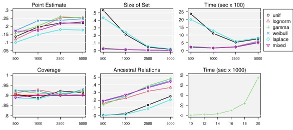
Figure 2. Top Left: % of times point estimate of ordering is correct. Top Middle: Avg proportion of all possible orderings included in $\hat{\Theta}(\mathbf{Y},\alpha=.9)$. Top Right: Avg time (sec$\times 100$) for each confidence set. Bottom Left: Coverage for $\hat{\Theta}(\mathbf{Y},\alpha=.9)$. Bottom Middle: Avg proportion of all ancestral relations which are included in $\mathcal{\hat{A}}_{\cap}$. Bottom Right: Median time (sec$\times 1000$) for each confidence set with $n=10,000$ and $p$ varying.

6.2. Confidence intervals with model selection uncertainty

We now consider CIs for causal effects which account for model uncertainty. We draw random graphs and data under the same setup in Section 6.1 with $p=10$, except we draw the magnitude of the linear coefficients from $\text{Gamma}(1/2,1)$, so the “signal strength” is fixed instead of decreasing with $n$ as before. We compute 80% CIs for the total effect of $Y_{4}$ onto $Y_{7}$ using Alg. 3. We contrast this with a naïve procedure that computes CIs using only the adjustment set implied by $\hat{\theta}$, the causal ordering estimated by DirectLiNGAM. Specifically, if $\hat{\theta}(4)<\hat{\theta}(7)$, then the naïve procedure uses an adjustment set of ${\rm pr}_{\hat{\theta}}(4)$ and returns the typical 80% CI for the regression coefficient of $Y_{4}$. When $\hat{\theta}(4)>\hat{\theta}(7)$, $7$ is estimated to be an non-descendant of $4$, so the returned CI is $0$.

Table 2 compares the empirical coverage and lengths of the proposed CIs and the naïve CIs. The proposed CIs have empirical coverage above the nominal rate. The “Adj” column shows the proportion of times the point estimate yields a valid adjustment set for the total effect. Given that these values are much smaller than $1$, it is unsurprising that the naïve CIs cover well below the nominal rate. Under gamma errors—when the model uncertainty is typically smaller—the proposed CIs have median length that is only 2-3 times larger than the naive procedure. However, in the Laplace setting where model uncertainty is larger, the median length is up to 5 times longer.

Table 2. Comparison of 80% CIs for the total effect of $Y_{4}$ onto $Y_{7}$. “MU” denotes CIs which account for model uncertainty; “NV” denotes naïve CIs

n	Gamma							Laplace
	Coverage		Avg Len		Med Len		Adj	Coverage		Avg Len		Med Len		Adj
	MU	NV	MU	NV	MU	NV		MU	NV	MU	NV	MU	NV
250	.97	.67	.81	.19	.55	.18	.37	.99	.59	1.1	.19	.74	.17	.25
500	.96	.63	.60	.14	.38	.13	.42	.99	.61	.86	.13	.60	.12	.36
1000	.97	.71	.37	.10	.24	.09	.51	.99	.64	.68	.10	.45	.09	.44
2000	.94	.71	.22	.07	.14	.06	.61	.97	.65	.46	.07	.30	.06	.54

6.3. Data example

We now analyze data consisting of the daily value-weighted average stock returns for 12 different industry portfolios from 2019 to 2022 ($n=1008$). All stocks from the NYSE, AMEX, and NASDAQ are placed into one of 12 different industries. Using DirectLiNGAM, the estimated causal ordering is: Utilities, Energy, Manufacturing, Business Equipment, Finance, Other, Telecomm, Consumer Non-Durable, Wholesale, Consumer Durables, Chemicals, Healthcare. The 95% confidence set of causal orderings returned for the data contains approximately $1/15,290$ of the $12!$ total orderings. The right panel in Fig. 3 summarizes the pairwise ancestral relationships for all non-rejected orderings, where darker shades of the $(u,v)$ element indicates that $v$ precedes $u$ in a larger proportion of non-rejected orderings.

Notably, Utilities is first in every non-rejected ordering so $\mathcal{\hat{A}}_{\cap}=\{(8,v)\,:\,v\neq 8\}$, which agrees with the point estimate. At first glance, this may seem odd; however, Utilities are often viewed as a proxy for bonds and directly capture the effect of changing interest rates and market uncertainty. From 2020 to 2022, the performance of American stock markets was largely driven by uncertainty around COVID-19 and federal monetary interventions. Thus, it makes sense that “Utitilies” are estimated to be an ancestor of all other industries.

Nonetheless, the other orderings in $\hat{\Theta}(\mathbf{Y},\alpha=.05)$ have causal implications which differ from the point estimate. We compute the Fréchet mean of $\hat{\Theta}(\mathbf{Y},\alpha=.05)$ using a distance between two orderings which counts the number of implied ancestral relations present in one ordering but not the other; i.e., $d(\theta,\theta^{\prime})=\left|\{(u,v)\,:\,u\in\text{pr}_{\theta}(v)\text{ and }u\not\in\text{pr}_{\theta^{\prime}}(v)\}\right|.$ The mean ordering is: Utilities, Wholesale, Consumer Non-durables, Healthcare, Chemicals, Finance, Energy, Business Equipment, Telecomm, Consumer Durables, Manufacturing, Other, and the left panel of Fig. 3 shows the distance from the Fréchet mean for all orderings in $\hat{\Theta}(\mathbf{Y},\alpha)$. The distance of the point estimate is indicated by the vertical line, and we observe that it is actually further from the mean than most other orderings in $\hat{\Theta}(\mathbf{Y},\alpha)$.

Finally, the naive 90% CI for the total effect of Energy onto Manufacturing is $(0.306,0.353)$. Furthermore, since Manufacturing precedes Chemicals in the estimated ordering, we would naively conclude that the total effect of Chemicals onto Manufacturing is $0$. In contrast, when accounting for model uncertainty, we produce a 90% CI for the total effect of Energy onto Manufacturing of $\{0\}\cup(0.040,0.128)\cup(0.171,0.291)\cup(0.301,0.358)$ and a CI for the effect of Chemicals onto Energy of $\{0\}\cup(0.101,0.909)\cup(0.973,1.101)$.

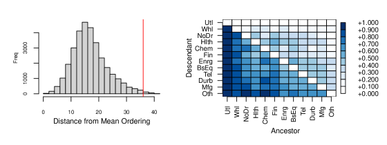
Figure 3. Left: distance from Fréchet mean to all other orderings in $\hat{\Theta}(\mathbf{Y},.05)$. The distance for the point estimate is indicated by the vertical line. Right: A darker shade of the $(u,v)$ cell indicates that $v$ precedes $u$ in a larger proportion of orderings in $\hat{\Theta}(\mathbf{Y},.05)$.

7. Discussion

We have proposed a procedure for quantifying uncertainty when estimating the causal structure. Our goodness-of-fit testing framework returns a confidence set that may be informative about the validity of the posited identification assumptions, as well as which causal orderings the identifying assumptions cannot rule out. The confidence set can also be used to compute various other objects of interest. Notably, this includes confidence intervals for causal effects that also account for model uncertainty and a sub/superset of ancestral relations. Our specific goodness-of-fit test is designed for models in which residuals are independent of regressors under the null hypothesis. Future work could extend this procedure to settings where causal sufficiency may not hold (Wang and Drton, 2020a, ).

While we believe the proposed approach has many desirable characteristics, there, of course, also are a few previously mentioned disadvantages which could be addressed in future work. Most notably, the primary disadvantage of our approach is the computational expense required to test the set of all possible orderings. While the proposed branch and bound procedure can handle medium-sized problems and could scale even larger with a careful parallel implementation, the approach is unlikely to scale too far beyond $p=20$. Nonetheless, we believe that this approach is a useful first step. We believe that this initial method is valuable for practitioners and hope it also spurs further research in statistical methodology for quantifying model uncertainty in estimating causal structures.

Appendix A Example of naive strategy

The following example examines the naive strategy of regressing a parent onto a child and directly testing independence of the residuals and regressors. Specifically, Table 3 shows that the naive procedure does not control the Type I error rate.

Example A.1.

Suppose $Y=(Y_{1},Y_{2})$ is generated as

$$Y_{1} \leftarrow\varepsilon_{1}, \varepsilon_{1}\sim\rm{gamma}(1,1)-1,$$

$$Y_{2} \leftarrow.5\times Y_{1}+\varepsilon_{2}, \varepsilon_{2}\sim\rm{gamma}(1,1)-1,$$

so that the true graph is $Y_{1}\rightarrow Y_{2}$. We consider two competing hypotheses which suppose $H_{0}:Y_{p}\rightarrow Y_{c}$ for $(p=1,c=2)$ or $(p=2,c=1)$, and we consider two testing approaches.

Direct approach: Regress $\mathbf{Y}_{c}$ onto $\mathbf{Y}_{p}$ to form the residuals $\bm{\hat{\eta}}_{c\setminus p}$, and subsequently test $\bm{\hat{\eta}}_{c\setminus p}\mathchoice{\mathrel{\hbox to0.0pt{$\displaystyle\perp$\hss}\mkern 2.0mu{\displaystyle\perp}}}{\mathrel{\hbox to0.0pt{$\textstyle\perp$\hss}\mkern 2.0mu{\textstyle\perp}}}{\mathrel{\hbox to0.0pt{$\scriptstyle\perp$\hss}\mkern 2.0mu{\scriptstyle\perp}}}{\mathrel{\hbox to0.0pt{$\scriptscriptstyle\perp$\hss}\mkern 2.0mu{\scriptscriptstyle\perp}}}\bm{Y}_{p}$ using dHSIC (Pfister et al.,, 2018) or $\tau^{\star}$ (Bergsma and Dassios,, 2014).

Sample splitting: Split the data into a training and test set. Using the training set, regress $\mathbf{Y}^{(train)}_{c}$ onto $\mathbf{Y}^{(train)}_{p}$ and estimate $\hat{\beta}_{c,p}$. Using the test set, form the residuals $\bm{\hat{\eta}}_{c\setminus p}=\mathbf{Y}^{(test)}_{p}-\hat{\beta}_{c,p}\mathbf{Y}^{(test)}_{c}$, and subsequently test $\bm{\hat{\eta}}_{c\setminus p}\mathchoice{\mathrel{\hbox to0.0pt{$\displaystyle\perp$\hss}\mkern 2.0mu{\displaystyle\perp}}}{\mathrel{\hbox to0.0pt{$\textstyle\perp$\hss}\mkern 2.0mu{\textstyle\perp}}}{\mathrel{\hbox to0.0pt{$\scriptstyle\perp$\hss}\mkern 2.0mu{\scriptstyle\perp}}}{\mathrel{\hbox to0.0pt{$\scriptscriptstyle\perp$\hss}\mkern 2.0mu{\scriptscriptstyle\perp}}}\bm{Y}^{(test)}_{p}$.

Table 3 shows the proportion of hypothesis tests that are rejected when the null is true ($H_{0}:Y_{1}\rightarrow Y_{2}$) and when the null is false ($H_{0}:Y_{2}\rightarrow Y_{1}$) for sample sizes of $n=100,1000$. We see that the naive tests with dHSIC or $\tau^{\star}$ (both the direct approach or sample splitting) do not control the Type I error rate. Under the direct approach, $\tau^{\star}$ has a Type I error rate close to the nominal rate when $n=100$, but when $n=1000$ and the test has more power, the Type I error rate is not controlled.

Table 3. Cols 2-6: empirical size of a level $\alpha=.1$ test. Cols 7-12: power of a level $\alpha=.1$ test. ‘Direct’ indicates the direct approach, ‘Split’ indicates the sample splitting approach, and ‘Prop’ indicates the proposed approach. ‘D’ indicates using the dHSIC statistic, $\tau$ indicates using the $\tau^{\star}$ statistic.

	$H_{0}:Y_{1}\rightarrow Y_{2}$					$H_{0}:Y_{2}\rightarrow Y_{1}$
	Direct		Split		Prop	Direct		Split		Prop
	D	$\tau$	D	$\tau$		D	$\tau$	D	$\tau$
$n=100$	0.15	0.11	0.23	0.32	0.10	1.00	1.00	0.97	0.94	0.64
$n=1000$	0.18	0.20	0.24	0.34	0.09	1.00	1.00	1.00	1.00	0.97

Appendix B Calibrating the test with a limiting Gaussian

We show that the asymptotic normal distribution of (3.3) may provide a poor approximation when $\varepsilon_{v}$ is far from Gaussian. Specifically, we consider log-normal data with $n=500$ and $p=5,10,\ldots,25$ and record the Type I error rate for a nominally $\alpha=.05$ test calibrated using the limiting Gaussian with a plug-in estimate of the variance. We see that this test performs quite poorly when compared to the tests calibrated by the oracle and proposed residual bootstrap distributions.

Table 4. The empirical size for 2000 replications of a nominally $\alpha=.05$ tests with $n=500$ when calibrating with the asymptotic distribution, the oracle distribution, and the proposed residual bootstrap distribution. All values are multiplied by 1000. The confidence interval with 2 standard errors is given in the parenthesis.

	$p=5$	10	15	20	25
Asymp	67 (56, 78)	78 (66, 90)	98 (84, 111)	102 (88, 115)	100 (87, 113)
Oracle	46 (36, 55)	46 (37, 56)	50 (40, 60)	50 (40, 60)	49 (39, 59)
Proposed	46 (37, 55)	51 (41, 61)	48 (39, 58)	56 (45, 66)	46 (37, 55)

We generated data for the simulation in the following way. Let $X\in\mathbb{R}^{p}$. We draw $X=\exp(Z)$ from a log-normal distribution where $Z\sim N(0,\Sigma)$ with $\Sigma_{v,v}=1$ and all off-diagonals $\Sigma_{u,v}=.2$. Let $\bm{X}$ denote the matrix where each row denotes an i.i.d observation of $X$ with $\bm{X}$ scaled and centered so each column has mean $0$ and variance $1$. Furthermore, let $\bm{\tilde{X}}$ denote the matrix $\bm{X}$ augmented with a column of $1$s for the intercept. We use a single test function $h(X_{v})=X_{v}^{2}$, and let $\bm{H}$ be the matrix where the $u$th column corresponds to a scaled and centered version of $h(X_{v})=X_{v}^{2}$.

We draw $\bm{Y}=\bm{X}\beta+\bm{\varepsilon}$ where $\beta_{v}=1$ for all $v$ and $\bm{\varepsilon}=(\varepsilon_{i}:i\in[n])$ where $\varepsilon_{i}=\exp(w_{i})-{\mathbb{E}}(\exp(w_{i}))$ is also log-normal with $w_{i}\sim N(0,\log(1+\sqrt{(}5))-\log(2))$ so that $\varepsilon_{i}$ has mean $0$ and variance $1$. We regress $Y$ onto $\tilde{X}$ (including an intercept) and let $\bm{\hat{\eta}}$ denote the resulting residuals. We also calculate, $\hat{\sigma}^{2}=\frac{\|\bm{\hat{\eta}}\|^{2}}{n-p}$, an unbiased estimate of the variance of $\varepsilon$

For the test calibrated by the asymptotic distribution, we then compare the test statistic $T_{2}=\|\frac{1}{n}\bm{H}^{T}\bm{\hat{\eta}}\|_{2}^{2}$ to the distribution of

(B.1) $$\left\|\frac{1}{\sqrt{n-p}}\bm{H}^{T}\left(I-\bm{\tilde{X}}(\bm{\tilde{X}}^{T}\bm{\tilde{X}})^{-1}\bm{\tilde{X}}^{T}\right)\bm{\check{\varepsilon}}_{v}\right\|_{2}^{2}$$

where each element of $\bm{\check{\varepsilon}}_{v}$ is drawn from $N(0,\hat{\sigma}^{2})$. Note that we divide by $\sqrt{n-p}$ instead of $n$ in the null distribution which should help lower the Type I error rate in finite samples. Indeed, this correction improves performance; however, even with this additional correction the Type I error is inflated.

For the test calibrated by the oracle distribution, we then compare the test statistic $T_{2}=\|\frac{1}{n}\bm{H}^{T}\bm{\hat{\eta}}\|_{2}^{2}$ to the distribution of

(B.2) $$\left\|\frac{1}{\sqrt{n-p}}\bm{H}^{T}\left(I-\bm{\tilde{X}}(\bm{\tilde{X}}^{T}\bm{\tilde{X}})^{-1}\bm{\tilde{X}}^{T}\right)\bm{\check{\varepsilon}}_{v}\right\|_{2}^{2}$$

where each element of $\bm{\check{\varepsilon}}_{v}$ is drawn from $\exp(w_{i})-{\mathbb{E}}(\exp(w_{i}))$ with $w_{i}\sim N(0,\log(1+\sqrt{(}5))-\log(2))$.

This entire procedure is replicated 2000 times with $n=500$ and $p=5,10,\ldots,25$. In Figure 4, we show the distribution of the resulting p-values for each procedure in each setting.

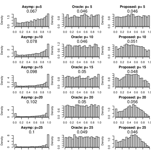
Figure 4. Comparison of p-values from tests calibrated by the estimated asymptotic normal distribution, the oracle distribution, and the proposed residual bootstrap distribution. Results show $2000$ replications with $n=500$ and various values of $p$. The empirical size for nominally $\alpha=.05$ tests are displayed under each title.

Appendix C Proofs for Section 4.3

Lemma 1

Let $\pi_{u,v}$ denote the total causal effect of $v$ onto $u$. Suppose $\hat{\Theta}(\mathbf{Y},\alpha/2)$ satisfies (1.2), and $C(S)$ is an asymptotically valid $1-\alpha/2$ confidence interval for the parameter of interest, conditional on $S$ being a valid adjustment set. Then, for the confidence interval produced by Alg. 3, $\lim_{n\rightarrow\infty}P(\pi_{u,v}\in\hat{C}_{\alpha})\geq 1-\alpha.$

Proof.

If $u\in{\rm an}(v)$, then for every $\theta\in\Theta(G)$, $\theta(u)<\theta(v)$. Fix an arbitrary $\theta\in\Theta(G)$. Let $S_{\theta}$ denote the appropriate adjustment set for the effect of interest given $\theta$ and let $C(S_{\theta})$ denote the $1-\alpha/2$ confidence interval for the effect of interest when using the adjustment set $S_{\theta}$. Then,

(C.1) $$\lim_{n\rightarrow\infty}P(\pi_{u,v}\in\hat{C}_{\alpha})\geq 1-\lim_{n\rightarrow\infty}P\left(\theta\not\in\hat{\Theta}(\mathbf{Y},\alpha/2)\cup\pi_{u,v}\not\in C(S_{\theta})\right)\geq 1-(\alpha/2+\alpha/2).$$

If $u\not\in{\rm an}(v)$, then $\pi_{v,u}=0$ and there exists a $\theta\in\Theta(G)$ such that $\theta(v)<\theta(u)$. Then,

(C.2) $$\lim_{n\rightarrow\infty}P(\pi_{u,v}\in\hat{C}_{\alpha})\geq 1-\lim_{n\rightarrow\infty}P(\theta\not\in\hat{\Theta}(\mathbf{Y},\alpha/2)\geq 1-\alpha/2,$$

which completes the proof. ∎

Lemma 2

Suppose $\hat{\Theta}(\mathbf{Y},\alpha)$ satisfies (1.2). Then, $\lim_{n\rightarrow\infty}P(\mathcal{\hat{A}}_{\cap}\subseteq\mathcal{A}\subseteq\mathcal{\hat{A}}_{\cup})\geq 1-2\alpha.$

Proof.

Suppose $\Theta(G)=\{\theta_{1}\}$ so that $|\Theta(G)|=1$. Then, by definition, $\theta_{1}(v)<\theta_{1}(u)$ for every $(u,v)\not\in\mathcal{A}$. Thus, $\theta_{1}\in\hat{\Theta}(\mathbf{Y},\alpha)$ implies that $\mathcal{A}_{\cap}\subseteq\mathcal{A}$. Similarly, since $\theta_{1}(u)<\theta_{1}(v)$ for every $(u,v)\in\mathcal{A}$ when $\theta_{1}\in\hat{\Theta}(\mathbf{Y},\alpha)$, then $\theta_{1}\in\hat{\Theta}(\mathbf{Y},\alpha)$ also implies that $\mathcal{A}\subseteq\mathcal{\hat{A}}_{\cup}$. If $\hat{\Theta}(\mathbf{Y},\alpha)$ satisfies Eq. (1.2), then $\theta_{1}\in\hat{\Theta}(\mathbf{Y},\alpha)$ occurs with probability bounded below by $1-\alpha$ as $n\rightarrow\infty$ so that

(C.3) $$\lim_{n\rightarrow\infty}P(\mathcal{\hat{A}}_{\cap}\subseteq\mathcal{A}\subseteq\mathcal{\hat{A}}_{\cup})\geq 1-\alpha.$$

Now consider the case where $|\Theta(G)|>1$. There exist a pair $\theta_{1},\theta_{2}\in\Theta(G)$ such that:

1. For every $(u,v)\in\mathcal{A}$, we have $\theta_{1}(u)<\theta_{1}(v)$ and $\theta_{2}(u)<\theta_{2}(v)$

2. For every $(u,v)\not\in\mathcal{A}$, we have $\theta_{1}(u)<\theta_{1}(v)$ and $\theta_{2}(v)<\theta_{2}(u)$.

Then, for every $(u,v)\not\in\mathcal{A}$ either $\theta_{1}(v)<\theta_{1}(u)$ or $\theta_{2}(v)<\theta_{2}(u)$. Thus, the event $\{\theta_{1}\in\hat{\Theta}(\mathbf{Y},\alpha)\}\cap\{\theta_{2}\in\hat{\Theta}(\mathbf{Y},\alpha)\}$ implies that $\mathcal{\hat{A}}_{\cap}\subseteq\mathcal{A}$. Furthermore, for every $(u,v)\in\mathcal{A}$, $\theta_{1}(v)<\theta_{1}(u)$. Thus, the event $\{\theta_{1}\in\hat{\Theta}(\mathbf{Y},\alpha)\}$ also implies $\mathcal{A}\subseteq\mathcal{\hat{A}}_{\cup}$. If $\hat{\Theta}(\mathbf{Y},\alpha)$ satisfies Eq. (1.2), then $\{\theta_{1}\in\hat{\Theta}(\mathbf{Y},\alpha)\}\cap\{\theta_{2}\in\hat{\Theta}(\mathbf{Y},\alpha)\}$ occurs with probability bounded below by $1-2\alpha$ as $n\rightarrow\infty$ so that

(C.4) $$\lim_{n\rightarrow\infty}P(\mathcal{\hat{A}}_{\cap}\subseteq\mathcal{A}\subseteq\mathcal{\hat{A}}_{\cup})\geq 1-2\alpha.$$

∎

Appendix D Confidence intervals for direct effects

Alg. 4 describes a procedure to calculate confidence intervals for direct effects which also incorporate model uncertainty. When estimating the direct effect of $v$ onto $u$, a valid adjustment set is ${\rm an}(u)$. Thus, this procedure is exactly the same as Alg. 3 except for the definition of $\mathcal{S}$.

Algorithm 4 Get $1-\alpha$ CI for the direct effect of $v$ onto $u$

1:for $S\in\mathcal{S}=\{S\,:\,S={\rm pr}_{\theta}(u)\text{ for some }\theta\in\hat{\Theta}(\mathbf{Y},\alpha/2)\text{ such that }\theta(v)<\theta(u)\}$ do

2:     Calculate $C(S)$, the $1-\alpha/2$ confidence interval for the coefficient of $Y_{v}$ when regressing $Y_{u}$ onto $Y_{S\cup\{v\}}$

3:end for

4:if $\theta(u)>\theta(v)$ for any $\theta\in\hat{\Theta}(\mathbf{Y},\alpha/2)$ then

5:     Return: $\hat{C}_{\alpha}=\{0\}\cup\{\bigcup_{S\in\mathcal{S}}C(S)\}$

6:else

7:     Return: $\hat{C}_{\alpha}=\bigcup_{S\in\mathcal{S}}C(S)$

8:end if

Appendix E Proofs for Section 5.1

We first give two intermediate lemmas which are needed for the proof of Theorem 1 and then prove Theorem 1.

Lemma 5 is a deterministic statement that decomposes the Wasserstein distance between the oracle distribution of $T$ and the residual bootstrap distribution of $T$ into the sum of the distance between $F^{(v)}$, the distribution of the errors, and $F_{n}^{(v)}$, the empirical distribution of the errors, as well as the distance between $F_{n}^{(v)}$ and, $\hat{F}_{n}^{(v)}$, the empirical distribution of the residuals. Since we fix $\theta$, to ease the notational burden, we will drop the ${\rm pr}_{\theta}(v)$ and let $\bm{\hat{\eta}}_{v}=\bm{\hat{\eta}}_{v\setminus{\rm pr}_{\theta}(v)}$. For notational simplicity, let $\mathbf{Z}\in\mathbb{R}^{n\times K}=\left(\phi_{k}(Y_{{\rm pr}_{\theta}(v),i})\,:\,k\in[K],\;i\in[n]\right)$ denote the matrix that contains the $K$ basis functions evaluated on the $n$ observations. Let $b\in\mathbb{R}^{K}$ denote the “linear coefficients” of $f_{v,K}$, so that $f_{v,K}=b\Phi_{v}^{(K)}b$,

Lemma 5.

For any $\mathbf{Y}$, $v\in V$, and ${\rm pr}_{\theta}(v)\subseteq V\setminus v$, let $\overline{h_{j}(\mathbf{Y}_{u})^{2}}=\frac{1}{n}\sum_{i}h_{j}(Y_{u,i})^{2}$ and $\overline{d^{2}_{v}}=\frac{1}{n}\sum_{i}d_{v,i}^{2}$. When ${\rm pa}(v)\subseteq{\rm pr}_{\theta}(v)\subseteq{\rm nd}(v)$, then

(E.1) $$d_{2}\left(T(\mathbf{Y}_{v},{\rm pr}_{\theta}(v);\mathbf{Y}),T(\mathbf{\tilde{Y}}_{v},{\rm pr}_{\theta}(v);\mathbf{Y})\right)^{2}\\ \leq 9J\left(\max_{\begin{subarray}{c}u\in{\rm pr}_{\theta}(v)\\ j\in[J]\end{subarray}}\overline{h_{j}(\mathbf{Y}_{u})^{2}}\right)\times\left[d_{2}(F^{(v)},F^{(v)}_{n})^{2}+d_{2}(F^{(v)}_{n},\hat{F}^{(v)}_{n})^{2}\right]\\ +3J\min\left(\overline{d^{2}}\max_{i,j,u}h_{j}(Y_{u,i})^{2},\left(\max_{\begin{subarray}{c}u\in{\rm pr}_{\theta}(v)\\ j\in[J]\end{subarray}}\overline{h_{j}(\mathbf{Y}_{u})^{2}}\right)\max d_{i}^{2}\right).$$

Proof.

Under the null hypothesis, the residuals when regressing $\mathbf{Y}_{v}$ onto $\mathbf{Z}$ are

(E.2) $$\hat{\bm{\eta}}_{v} =\mathbf{Y}_{v}-\mathbf{Z}\hat{b}=\mathbf{Z}(b-\hat{b})+\mathbf{d}_{v}+\bm{\varepsilon}_{v}$$

$$=\left(I-\mathbf{Z}\left[\mathbf{Z}^{T}\mathbf{Z}\right]^{-1}\mathbf{Z}^{T}\right)(\bm{\varepsilon}_{v}+\mathbf{d}_{v}).$$

Thus, for any realization $\mathbf{Y}_{{\rm pa}(v)}$ and $\bm{\varepsilon}_{v}$,

$$\tau_{j}(\mathbf{Y}_{v},u,{\rm pr}_{\theta}(v);\mathbf{Y})=\frac{1}{\sqrt{n}}h_{j}(\mathbf{Y}_{u})^{T}\left(I-\mathbf{Z}\left[\mathbf{Z}^{T}\mathbf{Z}\right]^{-1}\mathbf{Z}^{T}\right)(\bm{\varepsilon}_{v}+\bm{d}_{v}).$$

Let $\tilde{\bm{\eta}}_{v}=(\tilde{\eta}_{v,i})_{i\in[n]}$ where each element $\tilde{\eta}_{v,i}$ is drawn from $\hat{F}^{(v)}_{n}$, the empirical distribution of $\{\hat{\eta}_{v,i}\}_{i\in[n]}$, so that the bootstrapped data are $\mathbf{\tilde{Y}}_{v}=\mathbf{Z}\hat{b}+\tilde{\bm{\eta}}_{v}$. Let $\tilde{b}$ denote the estimated coefficients when regressing $\mathbf{\tilde{Y}}_{v}$ onto $\mathbf{Z}$ and let $\hat{\bm{\tilde{\eta}}}_{v}$ denote the corresponding residuals. Then we also have

(E.3) $$\hat{\bm{\tilde{\eta}}}_{v} =\mathbf{\tilde{Y}}_{v}-\mathbf{Z}\tilde{b}=\mathbf{Z}(\hat{b}-\tilde{b})+\bm{\tilde{\eta}}_{v}$$

$$=\left(I-\mathbf{Z}\left[\mathbf{Z}^{T}\mathbf{Z}\right]^{-1}\mathbf{Z}^{T}\right)\bm{\tilde{\eta}}_{v},$$

and

$$\tau_{j}(\mathbf{\tilde{Y}}_{v},u,{\rm pr}_{\theta}(v);\mathbf{Y})=\frac{1}{\sqrt{n}}h_{j}(\mathbf{Y}_{u})^{T}\left(I-\mathbf{Z}\left[\mathbf{Z}^{T}\mathbf{Z}\right]^{-1}\mathbf{Z}^{T}\right)\tilde{\bm{\eta}}_{v}.$$

Let $Q$ denote a joint distribution over $\varepsilon_{v,i}$ and $\tilde{\eta}_{v,i}$, which achieves the Wasserstein lower bound; i.e., $d_{2}(\varepsilon_{v,i},\tilde{\eta}_{v,i})^{2}=E_{Q}(|\varepsilon_{v,i}-\tilde{\eta}_{v,i}|^{2})$. In a slight abuse of notation, we will also use $Q$ to denote the distribution over $\tau_{j}(Y_{v},u,{\rm pa}(v);\mathbf{Y})$ and $\tau_{j}(\tilde{Y}_{v},u,{\rm pa}(v);\mathbf{Y})$, which is induced by conditioning on $\mathbf{Y}_{{\rm pr}_{\theta}(v)}$ and drawing $\varepsilon_{v,i}$ and $\tilde{\eta}_{v,i}$ from $Q$. Since $Q$ preserves the marginal distributions of $\varepsilon_{v,i}$ and $\tilde{\eta}_{v,i}$, it also preserves the marginal distributions of $\tau_{j}(Y_{v},u,{\rm pa}(v);\mathbf{Y})$ and $\tau_{j}(\tilde{Y}_{v},u,{\rm pa}(v);\mathbf{Y})$ for all $j$ and $u\in{\rm pr}_{\theta}(v)$.

Let $\tau_{v}=\{\tau(\mathbf{Y}_{v},u,{\rm pa}(v);\mathbf{Y})\}_{u\in{\rm pr}_{\theta}(v)}$ and $\tilde{\tau}_{v}=\{\tau(\mathbf{\tilde{Y}}_{v},u,{\rm pa}(v);\mathbf{Y})\}_{u\in{\rm pr}_{\theta}(v)}$. For $T_{1}$, we have

(E.4) $$d_{2} \left(T_{1}(\mathbf{Y}_{v},{\rm pr}_{\theta}(v);\mathbf{Y}),T_{1}(\mathbf{\tilde{Y}}_{v},{\rm pr}_{\theta}(v);\mathbf{Y})\right)^{2}\leq E_{Q}\left[\left(T_{1}(\mathbf{Y}_{v}{\rm pr}_{\theta}(v);\mathbf{Y})-T_{1}(\mathbf{\tilde{Y}}_{v}{\rm pr}_{\theta}(v);\mathbf{Y})\right)^{2}\right]$$

$$={\mathbb{E}}_{Q}\left[\left(\frac{1}{|{\rm pr}_{\theta}(v)|}|\tau_{v}|_{1}-\frac{1}{|{\rm pr}_{\theta}(v)|}|\tilde{\tau}_{v}|_{1}\right)^{2}\right]\stackrel{{\scriptstyle(i)}}{{\leq}}{\mathbb{E}}_{Q}\left[\left(\frac{1}{|{\rm pr}_{\theta}(v)|}|\tau_{v}-\tilde{\tau}_{v}|_{1}\right)^{2}\right]$$

$$={\mathbb{E}}_{Q}\left[\frac{1}{|{\rm pr}_{\theta}(v)|^{2}}\left(\sum_{u\in{\rm pr}_{\theta}(v)}|\tau(\mathbf{Y}_{v},u,{\rm pr}_{\theta}(v);\mathbf{Y})-\tau(\mathbf{\tilde{Y}}_{v},u,{\rm pr}_{\theta}(v);\mathbf{Y})|\right)^{2}\right]$$

$$=\frac{1}{|{\rm pr}_{\theta}(v)|^{2}}\sum_{u\in{\rm pr}_{\theta}(v)}{\mathbb{E}}_{Q}\left[\left(\tau(\mathbf{Y}_{v},u,{\rm pr}_{\theta}(v);\mathbf{Y})-\tau(\mathbf{\tilde{Y}}_{v},u,{\rm pr}_{\theta}(v);\mathbf{Y})\right)^{2}\right]$$

$$\quad+\frac{1}{|{\rm pr}_{\theta}(v)|^{2}}\sum_{u_{1}\neq u_{2}}{\mathbb{E}}_{Q}\left[\left|\tau(\mathbf{Y}_{v},u_{1},{\rm pr}_{\theta}(v);\mathbf{Y})-\tau(\mathbf{\tilde{Y}}_{v},u_{1},{\rm pr}_{\theta}(v);\mathbf{Y})\right|\left|\tau(\mathbf{Y}_{v},u_{2},{\rm pr}_{\theta}(v);\mathbf{Y})-\tau(\mathbf{\tilde{Y}}_{v},u_{2},{\rm pr}_{\theta}(v);\mathbf{Y})\right|\right]$$

$$\leq\max_{u\in{\rm pr}_{\theta}(v)}{\mathbb{E}}_{Q}\left[\left(\tau(\mathbf{Y}_{v},u,{\rm pr}_{\theta}(v);\mathbf{Y})-\tau(\mathbf{\tilde{Y}}_{v},u,{\rm pr}_{\theta}(v);\mathbf{Y})\right)^{2}\right].$$

The inequality in (i) holds because of the reverse triangle inequality. Similarly, for $T_{2}$, we have

(E.5) $$d_{2} \left(T_{2}(\mathbf{Y}_{v},{\rm pr}_{\theta}(v);\mathbf{Y}),T_{2}(\mathbf{\tilde{Y}}_{v},{\rm pr}_{\theta}(v);\mathbf{Y})\right)^{2}\leq E_{Q}\left[\left(T_{2}(\mathbf{Y}_{v};,{\rm pr}_{\theta}(v);\mathbf{Y})-T_{2}(\mathbf{\tilde{Y}}_{v},{\rm pr}_{\theta}(v);\mathbf{Y})\right)^{2}\right]$$

$$={\mathbb{E}}_{Q}\left[\left(\frac{1}{\sqrt{|{\rm pr}_{\theta}(v)|}}|\tau_{v}|_{2}-\frac{1}{\sqrt{|{\rm pr}_{\theta}(v)|}}|\tilde{\tau}_{v}|_{2}\right)^{2}\right]\leq{\mathbb{E}}_{Q}\left[\left(\frac{1}{\sqrt{|{\rm pr}_{\theta}(v)|}}|\tau_{v}-\tilde{\tau}_{v}|_{2}\right)^{2}\right]$$

$$=\frac{1}{|{\rm pr}_{\theta}(v)|}\sum_{u\in{\rm pr}_{\theta}(v)}{\mathbb{E}}_{Q}\left[\left(\tau(\mathbf{Y}_{v},u,{\rm pr}_{\theta}(v);\mathbf{Y})-\tau(\mathbf{\tilde{Y}}_{v},u,{\rm pr}_{\theta}(v);\mathbf{Y})\right)^{2}\right]$$

$$\leq\max_{u}{\mathbb{E}}_{Q}\left[\left(\tau(\mathbf{Y}_{v},u,{\rm pr}_{\theta}(v);\mathbf{Y})-\tau(\mathbf{\tilde{Y}}_{v},u,{\rm pr}_{\theta}(v);\mathbf{Y})\right)^{2}\right].$$

Now we examine the quantity $E_{Q}\left\{\left[\tau(\mathbf{Y}_{v},u,{\rm pr}_{\theta}(v);\mathbf{Y})-\tau(\mathbf{\tilde{Y}}_{v},u,{\rm pr}_{\theta}(v);\mathbf{Y})\right]^{2}\right\}$ for any $u\in{\rm pr}_{\theta}(v)$. Let

$$\bm{A}_{j}=\frac{1}{\sqrt{n}}h_{j}(\mathbf{Y}_{u})^{T}\left(I-\mathbf{Z}\left[\mathbf{Z}^{T}\mathbf{Z}\right]^{-1}\mathbf{Z}^{T}\right)$$

so that $\tau_{j}(\mathbf{Y}_{v},u,{\rm pr}_{\theta}(v),\mathbf{Y})=\bm{A}_{j}(\bm{\varepsilon}_{v}+\mathbf{d}_{v})$ and $\tau(\mathbf{Y}_{v},u,{\rm pr}_{\theta}(v),\mathbf{Y})=\sqrt{\sum_{j}\left(\bm{A}_{j}(\bm{\varepsilon}_{v}+\mathbf{d}_{v})\right)^{2}}$. We then have

(E.6) $${\mathbb{E}}_{Q} \left\{\left[\tau(\mathbf{Y}_{v},u,{\rm pr}_{\theta}(v);\mathbf{Y})-\tau(\mathbf{\tilde{Y}}_{v},u,{\rm pr}_{\theta}(v);\mathbf{Y})\right]^{2}\right\}$$

$$={\mathbb{E}}_{Q}\left\{\left(\left|\{\bm{A}_{j}(\bm{\varepsilon}_{v}+\mathbf{d}_{v})\}_{j}\right|_{2}-\left|\{\bm{A}_{j}\mathbf{\tilde{\eta}}_{v}\}_{j}\right|_{2}\right)^{2}\right\}$$

$$\leq{\mathbb{E}}_{Q}\left\{\left|\{\bm{A}_{j}(\bm{\varepsilon}_{v}+\mathbf{d}_{v})-\bm{A}_{j}\mathbf{\tilde{\eta}}_{v}\}_{j}\right|^{2}_{2}\right\}$$

$$={\mathbb{E}}_{Q}\left\{\sum_{j}\left(\bm{A}_{j}((\bm{\varepsilon}_{v}+\mathbf{d}_{v})-\mathbf{\tilde{\eta}}_{v})\right)^{2}\right\}$$

$$\leq J\max_{j}{\mathbb{E}}_{Q}\left\{\left(\bm{A}_{j}((\bm{\varepsilon}_{v}+\mathbf{d}_{v})-\mathbf{\tilde{\eta}}_{v})\right)^{2}\right\}$$

$$\leq J\max_{j}{\mathbb{E}}_{Q}\left\{3\left(\bm{A}_{j}((\bm{\varepsilon}_{v}-\mathbf{\tilde{\eta}}_{v})\right)^{2}\right\}+J\max_{j}{\mathbb{E}}_{Q}\left\{3\left(\bm{A}_{j}\mathbf{d}_{v}\right)^{2}\right\}$$

$$=3J\max_{j}{\mathbb{E}}_{Q}\left\{\bm{A}_{j}(\bm{\varepsilon}_{v}-\mathbf{\tilde{\eta}}_{v})(\bm{\varepsilon}_{v}-\mathbf{\tilde{\eta}}_{v})^{T}\bm{A}_{j}^{T}\right\}+3J\max_{j}{\mathbb{E}}_{Q}\left\{\left(\bm{A}_{j}\mathbf{d}_{v}\right)^{2}\right\}.$$

As each draw is independent and ${\mathbb{E}}[\varepsilon_{v,i}]={\mathbb{E}}[\tilde{\eta}_{v,i}]=0$, we have ${\mathbb{E}}\left[(\varepsilon_{v,i}-\tilde{\eta}_{v,i})(\varepsilon_{v,j}-\tilde{\eta}_{v,j})\right]=0$. Thus, for the first term in (E.6), we have

$$3J \max_{j}{\mathbb{E}}_{Q}\left\{\bm{A}_{j}(\bm{\varepsilon}_{v}-\mathbf{\tilde{\eta}}_{v})(\bm{\varepsilon}_{v}-\mathbf{\tilde{\eta}}_{v})^{T}\bm{A}_{j}^{T}\right\}$$

$$=3E_{Q}[(\varepsilon_{v,i}-\tilde{\eta}_{v,i})^{2}]\times J\max_{j}\frac{1}{n}h_{j}(\mathbf{Y}_{u})^{T}\left(I-\mathbf{Z}\left[\mathbf{Z}^{T}\mathbf{Z}\right]^{-1}\mathbf{Z}^{T}\right)\left(I-\mathbf{Z}\left[\mathbf{Z}^{T}\mathbf{Z}\right]^{-1}\mathbf{Z}^{T}\right)^{T}h_{j}(\mathbf{Y}_{u})$$

$$\leq 3\left(E_{Q}((\varepsilon_{v,i}-\tilde{\eta}_{v,i})^{2})\right)J\max_{j}\frac{1}{n}h_{j}(\mathbf{Y}_{u})^{T}h_{j}(\mathbf{Y}_{u}),$$

since $\left(I-\mathbf{Z}\left[\mathbf{Z}\mathbf{Z}^{T}\right]^{-1}\mathbf{Z}^{T}\right)$ is idempotent. For the second term in (E.6), we have

$$(\bm{A}_{j}\mathbf{d}_{v})^{2} =\|\frac{1}{\sqrt{n}}h_{j}(\mathbf{Y}_{u})^{T}\left(I-\mathbf{Z}\left[\mathbf{Z}^{T}\mathbf{Z}\right]^{-1}\mathbf{Z}^{T}\right)\mathbf{d}_{v}\|^{2}$$

$$=\frac{1}{n}\sum_{i}(h_{j}(Y_{u,i}))^{2}\left(\left[(I-\mathbf{Z}\left[\mathbf{Z}^{T}\mathbf{Z}\right]^{-1}\mathbf{Z}^{T})\mathbf{d}_{v}\right]_{i}\right)^{2}$$

$$\leq\frac{1}{n}\max_{i}h_{j}(Y_{u,i})^{2}\sum_{i}\left(\left[(I-\mathbf{Z}\left[\mathbf{Z}^{T}\mathbf{Z}\right]^{-1}\mathbf{Z}^{T})\mathbf{d}_{v}\right]_{i}\right)^{2}$$

$$=\max_{i}h_{j}(Y_{u,i})^{2}\|\frac{1}{\sqrt{n}}(I-\mathbf{Z}\left[\mathbf{Z}^{T}\mathbf{Z}\right]^{-1}\mathbf{Z}^{T})\mathbf{d}_{v}\|_{2}^{2}$$

$$\leq\max_{i}h_{j}(Y_{u,i})^{2}\frac{1}{n}\mathbf{d}_{v}^{T}\mathbf{d}_{v}=\max_{i}h_{j}(Y_{u,i})^{2}\overline{d^{2}}.$$

A similar argument can be made to show that $(\bm{A}_{j}\mathbf{d}_{v})^{2}\leq\left(\max_{j\in[J]}\overline{h_{j}(\mathbf{Y}_{u})^{2}}\right)\max d_{i}^{2}$. Combining the last two displays with (E.6), we have

(E.7) $${\mathbb{E}}_{Q} \left\{\left[\tau(\mathbf{Y}_{v},u,{\rm pr}_{\theta}(v);\mathbf{Y})-\tau(\mathbf{\tilde{Y}}_{v},u,{\rm pr}_{\theta}(v);\mathbf{Y})\right]^{2}\right\}$$

$$\leq 3\left(E_{Q}((\varepsilon_{v,i}-\tilde{\eta}_{v,i})^{2})\right)J\max_{j}\overline{h_{j}(\mathbf{Y}_{u})^{2}}+3J\min\left(\overline{d^{2}}\max_{i,j}h_{j}^{2}(Y_{u,i}),\left(\max_{j\in[J]}\overline{h_{j}(\mathbf{Y}_{u})^{2}}\right)\max d_{i}^{2}\right).$$

By construction, the distribution $Q$ achieves the Wasserstein-2 lower bound, so $E_{Q}\left[(\varepsilon_{v,i}-\tilde{\eta}_{v,i})^{2})\right]=d_{2}(F^{(v)},\hat{F}_{n}^{(v)})^{2}$. Thus, for all $u\in{\rm pr}_{\theta}(v)$,

(E.8) $${\mathbb{E}}_{Q} \left\{\left[\tau(\mathbf{Y}_{v},u,{\rm pr}_{\theta}(v);\mathbf{Y})-\tau(\mathbf{\tilde{Y}}_{v},u,{\rm pr}_{\theta}(v);\mathbf{Y})\right]^{2}\right\}$$

$$\leq 3d_{2}\left(F^{(v)},\hat{F}^{(v)}_{n}\right)^{2}J\max_{j}\overline{h_{j}(\mathbf{Y}_{u})^{2}}+3J\min\left(\overline{d^{2}}\max_{i,j}h_{j}(Y_{u,i}),\left(\max_{j\in[J]}\overline{h_{j}(\mathbf{Y}_{u})^{2}}\right)\max d_{i}^{2}\right).$$

Using the triangle inequality to decompose the Wasserstein distance, we have

(E.9) $$d_{2} \left(T(\mathbf{Y}_{v},{\rm pr}_{\theta}(v);\mathbf{Y}),T(\mathbf{\tilde{Y}}_{v},{\rm pr}_{\theta}(v);\mathbf{Y})\right)^{2}$$

$$\leq 3J\max_{u,j}\overline{h_{j}(\mathbf{Y}_{u})^{2}}\times d_{2}\left(F^{(v)},\hat{F}^{(v)}_{n}\right)^{2}+3J\min\left(\overline{d^{2}}\max_{i,j}h_{j}(Y_{u,i}),\left(\max_{j\in[J]}\overline{h_{j}(\mathbf{Y}_{u})^{2}}\right)\max d_{i}^{2}\right)$$

$$\leq 9J\max_{u,j}\overline{h_{j}(\mathbf{Y}_{u})^{2}}\times\left(d_{2}(F^{(v)},F^{(v)}_{n})^{2}+d_{2}(F^{(v)}_{n},\hat{F}^{(v)}_{n})^{2}\right)$$

$$\qquad+3J\min\left(\overline{d^{2}}\max_{i,j}h_{j}(Y_{u,i}),\left(\max_{j\in[J]}\overline{h_{j}(\mathbf{Y}_{u})^{2}}\right)\max d_{i}^{2}\right),$$

which completes the proof. ∎

Lemma 6 provides a deterministic bound on $d_{2}(F^{(v)}_{n},\hat{F}^{(v)}_{n})^{2}$, which represents the squared Wasserstein distance between the empirical distribution of the errors and the residuals.

Lemma 6.

We have

(E.10) $$d_{2}\left(F_{n}^{(v)},\hat{F}_{n}^{(v)}\right)^{2} \leq 3\left(K\sigma_{v}^{2}/n+\left|\frac{1}{n}\bm{\varepsilon}_{v}^{T}\mathbf{Z}(\mathbf{Z}^{T}\mathbf{Z})^{-1}\mathbf{Z}^{T}\bm{\varepsilon}_{v}-{\mathbb{E}}\left(\frac{1}{n}\bm{\varepsilon}_{v}^{T}\mathbf{Z}(\mathbf{Z}^{T}\mathbf{Z})^{-1}\mathbf{Z}^{T}\bm{\varepsilon}_{v}\right)\right|+\frac{2}{n}\mathbf{d}_{v}^{T}\mathbf{d}_{v}\right),$$

where ${\rm var}(\varepsilon_{v})=\sigma_{v}^{2}$, $F_{n}^{(v)}$ denotes the empirical distribution of errors for $v$, and $\hat{F}_{n}^{(v)}$ denotes the empirical distribution of residuals for $v$.

Proof.

Let $\varepsilon_{v,i}$ be the $i$th realized error and $\hat{\eta}_{v,i}$ be the corresponding residual. Then

(E.11) $$\varepsilon_{v,i}-\hat{\eta}_{v,i}=\varepsilon_{v,i}-\left(\mathbf{Z}_{i}^{T}b+d_{i}+\varepsilon_{v,i}-\mathbf{Z}_{i}^{T}\hat{b}\right) =\mathbf{Z}_{i}^{T}\left(\hat{b}-b\right)-d_{i}$$

$$=\mathbf{Z}_{i}^{T}\left[(\mathbf{Z}^{T}\mathbf{Z})^{-1}\mathbf{Z}^{T}\left(\mathbf{Z}b+\bm{\varepsilon}_{v}+\mathbf{d}_{v}\right)-b\right]$$

$$=\mathbf{Z}_{i}^{T}\left[(\mathbf{Z}^{T}\mathbf{Z})^{-1}\mathbf{Z}^{T}(\bm{\varepsilon}_{v}+\mathbf{d}_{v})\right]-d_{i}.$$

Suppose $(s_{1},s_{2})$ are drawn from a distribution $Q$ which is the uniform distribution over the pairs $\left\{\varepsilon_{v,i},\hat{\eta}_{v,i}\right\}_{i\in[n]}$. The marginal distributions of $s_{1}$ and $s_{2}$ are $F_{n}$ and $\hat{F}_{n}$, respectively. Then

(E.12) $${\mathbb{E}}_{Q}\left((s_{1}-s_{2})^{2}\right) =\frac{1}{n}\sum_{i}\left(\mathbf{Z}_{i}^{T}\left[(\mathbf{Z}^{T}\mathbf{Z})^{-1}\mathbf{Z}^{T}(\bm{\varepsilon}_{v}+\mathbf{d}_{v})\right]-d_{i}\right)^{2}$$

$$\leq\frac{3}{n}\sum_{i}(\bm{\varepsilon}_{v}+\mathbf{d}_{v})^{T}\mathbf{Z}(\mathbf{Z}^{T}\mathbf{Z})^{-1}(\mathbf{Z}_{i}\mathbf{Z}_{i}^{T})(\mathbf{Z}^{T}\mathbf{Z})^{-1}\mathbf{Z}^{T}(\bm{\varepsilon}_{v}+\mathbf{d}_{v})+\frac{3}{n}\sum_{i}d_{i}^{2}$$

$$=\frac{3}{n}\bm{\varepsilon}_{v}^{T}\mathbf{Z}(\mathbf{Z}^{T}\mathbf{Z})^{-1}\mathbf{Z}^{T}\bm{\varepsilon}_{v}+\frac{3}{n}\mathbf{d}_{v}^{T}(I+\mathbf{Z}(\mathbf{Z}^{T}\mathbf{Z})^{-1}\mathbf{Z}^{T})\mathbf{d}_{v}.$$

Since $\mathbf{Z}(\mathbf{Z}^{T}\mathbf{Z})^{-1}\mathbf{Z}^{T}$ is an idempotent matrix with rank $K$ that is independent of $\bm{\varepsilon}_{v}$, we have ${\mathbb{E}}\left(\bm{\varepsilon}_{v}^{T}\mathbf{Z}(\mathbf{Z}^{T}\mathbf{Z})^{-1}\mathbf{Z}^{T}\bm{\varepsilon}_{v}\right)=K\sigma_{v}^{2}$, $\|I+\mathbf{Z}(\mathbf{Z}^{T}\mathbf{Z})^{-1}\mathbf{Z}^{T}\|_{2}\leq 2$, and $\mathbf{d}_{v}^{T}(I+\mathbf{Z}(\mathbf{Z}^{T}\mathbf{Z})^{-1}\mathbf{Z}^{T})\mathbf{d}_{v}\leq 2\mathbf{d}_{v}^{T}\mathbf{d}_{v}$. Thus,

(E.13) $${\mathbb{E}}_{Q}\left((s_{1}-s_{2})^{2}\right)\leq 3\left(K\sigma_{v}^{2}/n+\left|\frac{1}{n}\bm{\varepsilon}_{v}\mathbf{Z}(\mathbf{Z}\mathbf{Z}^{T})^{-1}\mathbf{Z}\bm{\varepsilon}_{v}^{T}-{\mathbb{E}}\left(\frac{1}{n}\bm{\varepsilon}_{v}\mathbf{Z}(\mathbf{Z}\mathbf{Z}^{T})^{-1}\mathbf{Z}\bm{\varepsilon}_{v}^{T}\right)\right|+\frac{2}{n}\mathbf{d}_{v}^{T}\mathbf{d}_{v}\right).$$

Since the marginal distributions of $s_{1}$ and $s_{2}$ under $Q$ are $F_{n}$ and $\hat{F}_{n}$, we have $d_{2}\left(F_{n},\hat{F}_{n}\right)^{2}\leq{\mathbb{E}}_{Q}\left((s_{1}-s_{2})^{2}\right)$, which completes the proof. ∎

Theorem 1

Suppose that $p\leq K<n$ with $K=o(n)$. Furthermore, there exist constants $0<M_{1},M_{2},M_{3}<\infty$ such that for all $v\in V$ and $j\in[J]$, $\varepsilon_{v}\sim F^{(v)}$ with $\|\varepsilon_{v}\|_{\Psi_{1}}\leq M_{1}$, ${\rm var}(\varepsilon_{v})<M_{2}$, ${\mathbb{E}}(h_{j}(Y_{v})^{2})\leq M_{2}$ and $\|h_{j}(Y_{v})\|_{\Psi_{(1/J_{1})}}\leq M_{3}$ for some $1/2\leq J_{1}<\infty$.

Let $d^{\star}=\max_{v}\overline{d_{v}^{2}}$. Then, for any causal ordering $\theta$ consistent with DAG $G$, with probability $1-o(1)$, $\max_{v}d_{2}\left[T_{s}(\mathbf{Y}_{v},{\rm pr}_{\theta}(v);\mathbf{Y}),T(\mathbf{\tilde{Y}}_{v},{\rm pr}_{\theta}(v);\mathbf{Y})\right]^{2}$ is less than

(E.14) $$\footnotesize 27J(M_{2}+\log(p)/\sqrt{n})(KM_{2}/n+2\log(n)/\sqrt{n}+2d^{\star})+3Jd^{\star}(M_{2}+\log^{3J_{1}}(pJn)).$$

Proof.

Below we use $\mathbf{Z}_{v}\in\mathbb{R}^{n\times K_{v}}$ to denote to $\Phi^{(K_{v})}_{v}$ evaluated on $\mathbf{Y_{{\rm pr}_{\theta}(v)}}$; this is similar to our previous use of $\mathbf{Z}$, but we have added the additional subscript $v$ to denote that $\mathbf{Z}_{v}$ differs depending on $v$.

Suppose that there exist $\delta_{1},\delta_{2},\delta_{3},\delta_{4},\delta_{5}>0$ such that for all $v\in V$:

1. $\left|\frac{1}{n}\bm{\varepsilon}_{v}^{T}\mathbf{Z}_{v}(\mathbf{Z}_{v}^{T}\mathbf{Z}_{v})^{-1}\mathbf{Z}_{v}^{T}\bm{\varepsilon}_{v}-{\mathbb{E}}\left(\frac{1}{n}\bm{\varepsilon}_{v}^{T}\mathbf{Z}_{v}(\mathbf{Z}_{v}^{T}\mathbf{Z}_{v})^{-1}\mathbf{Z}_{v}^{T}\bm{\varepsilon}_{v}\right)\right|\leq\delta_{1}$;

2. $d_{2}(F^{(v)}_{n},F^{(v)})^{2}\leq\delta_{2}$;

3. $\max_{j}\overline{h_{j}(Y_{v})^{2}}\leq M_{2}+\delta_{3}$; and

4. $\max_{v,j,i}h_{j}(Y_{v,i})^{2}\leq M_{2}+\delta_{4}$.

Then by Lemma 5 and Lemma 6, we have

(E.15) $$\max_{v}d_{2}\left[T(\mathbf{Y}_{v},{\rm pr}_{\theta}(v);\mathbf{Y}),T(\mathbf{\tilde{Y}}_{v},{\rm pr}_{\theta}(v);\mathbf{Y})\right]^{2}\\ \leq 27J(M_{2}+\delta_{3})(KM_{2}/n+\delta_{1}+\delta_{2}+2d^{\star})+3Jd^{\star}(M_{2}+\delta_{4}).$$

We proceed to show that the above four conditions hold with the desired probability.

Condition (i): Let $\mathbf{A}_{v}=\mathbf{Z}_{v}(\mathbf{Z}_{v}^{T}\mathbf{Z}_{v})^{-1}\mathbf{Z}_{v}^{T}$. Note that $\mathbf{A}_{v}$ is a projection matrix of rank $K_{v}\leq K$. Therefore, we have ${\mathbb{E}}\left(n^{-1}\bm{\varepsilon}_{v}^{T}\mathbf{A}_{v}\bm{\varepsilon}_{v}\right)=\sigma^{2}_{v}K_{v}/n\leq M_{2}K/n$, $\|\mathbf{A}_{v}\|_{F}^{2}=K_{v}$, and $\|\mathbf{A}_{v}\|_{2}=1$. Setting $\delta_{1}=\log(p)/\sqrt{n}$, we have

$$P\left(\max_{v\in V}\left|\frac{1}{n}\bm{\varepsilon}_{v}^{T}\mathbf{A}_{v}\bm{\varepsilon}_{v}-{\mathbb{E}}\left(n^{-1}\bm{\varepsilon}_{v}^{T}\mathbf{A}_{v}\bm{\varepsilon}_{v}\right)\right|\geq\delta_{1}\right)\\ \leq 2p\exp\left(-\frac{c_{1}}{M_{1}^{4}}\min\left\{\frac{n\log^{2}(p)}{K},n^{1/4}\log^{1/2}(p)\right\}\right)$$

for some constant $c_{1}$ using Proposition 1.1 of Götze et al., (2021).

Condition (ii): Theorem 2 of Fournier and Guillin, (2015) states that for any $\zeta\in(0,1)$, we have

$$P\left(d_{2}\left(F^{(v)},F^{(v)}_{n}\right)^{2}\geq\delta_{2}\right)\\ \leq\left[\exp\left(-c_{2}n\delta_{2}^{2}\right)+\exp\left(-c_{2}(n\delta_{2})^{(1-\zeta)/2}\right)\right]1_{\{\delta_{2}\leq 1\}}+\exp\left(-c_{2}(n\delta_{2})^{1/2}\right)1_{\{\delta_{2}>1\}},$$

where the constant $c_{2}$ depends on $M_{1}$. Setting $\delta_{2}=\log(n)/\sqrt{n}$, $\zeta=1/2$, and using the union bound, we have

(E.16) $$P\left(\max_{v\in V}d_{2}\left(F^{(v)},F^{(v)}_{n}\right)^{2}\geq\delta_{2}\right)\leq cp/n.$$

Condition (iii): By assumption $\|h_{j}(Y_{v})\|_{\Psi_{(1/J_{1})}}\leq M_{3}$. Therefore, $\|h_{j}^{2}(Y_{v})\|_{\Psi_{1/(2J_{1})}}\leq M_{3}^{2}$ and, by Corollary 1.4 of Götze et al., (2021),

$$P(|\overline{h_{j}(Y_{v})^{2}}-{\mathbb{E}}(h_{j}(Y_{v})^{2})|\geq\delta_{3})\leq 2\exp\left(-c_{3}\min\left(\frac{\delta_{3}^{2}}{M_{3}^{4}(1/n)},\left[\frac{\delta_{3}}{M_{3}^{2}(1/n)}\right]^{1/(2J_{1})}\right)\right),$$

where $c_{3}$ is a constant that depends on $J_{1}$. Setting $\delta_{3}=\log(p)/\sqrt{n}$ and using the union bound, we have

(E.17) $$P(\max_{v,j}\overline{h_{j}(Y_{v})^{2}}\geq M_{2}+\delta_{3}) \leq pJ\exp\left(-c_{3}\left(\frac{\sqrt{n}\log(p)}{M_{3}^{2}}\right)^{1/(2J_{1})}\right).$$

Condition (iv): Since $h_{j}(Y_{{\rm pa}(v),i})^{2}$ is sub-Weibull $1/(2J_{1})$ with Orlicz norm of $M_{3}^{2}$, so we apply Corollary 1.4 of Götze et al., (2021). Letting $\delta_{4}=\log^{3J_{1}}(pJn)$, we have by a simple union bound

(E.18) $$P(\max_{v,j,i}h_{j}(Y_{v,i})^{2}\geq M_{2}+\delta_{4}) \leq pnJ\exp\left(-\left[\min\left(\frac{\log(pJn)^{6J_{1}}}{M_{3}^{4}},\frac{\log(pJn)^{3/2}}{M_{3}^{1/J_{1}}}\right)\right]\right).$$

∎

Corollary 1 (Known finite basis)

Suppose that conditions of Theorem 1 are satisfied. If each $f_{v}$ belongs to a known finite-dimensional basis, then with probability $1-o(1)$

$$\small\max_{v}d_{2}\left[T_{s}(\mathbf{Y}_{v},{\rm pr}_{\theta}(v);\mathbf{Y}),T_{s}(\mathbf{\tilde{Y}}_{v},{\rm pr}_{\theta}(v);\mathbf{Y})\right]^{2}\leq 27J\left(M_{2}+\frac{\log(p)}{\sqrt{n}}\right)\left(KM_{2}/n+\frac{2\log(n)}{\sqrt{n}}\right).$$

Proof.

The proof immediately follows from Theorem 1 by setting $d^{\star}=0$. ∎

Corollary 2 (Sieve basis)

Suppose that conditions of Theorem 1 are satisfied. Furthermore, suppose that a finite-dimensional basis for each $f_{v}$ is not known a priori, but there exists $K^{\star}$ such that for all $K>K^{\star}$, $\|f_{v}(Y_{{\rm pr}_{\theta}(v)})-f_{v,K}(Y_{{\rm pr}_{\theta}(v)})\|_{\Psi_{1}}\leq M_{1}$, and $\max_{v}{\mathbb{E}}(d_{v}^{2})<K^{-r}$ for some $r>0$. Letting $K=n^{1/(1+r)}$, we have with probability $1-o(1)$ for some constant $c$ which depends on $M_{1},M_{2}$,

(E.19) $$\footnotesize\max_{v}d_{2}\left[T_{s}(\mathbf{Y}_{v},{\rm pr}_{\theta}(v);\mathbf{Y}),T_{s}(\mathbf{\tilde{Y}}_{v},{\rm pr}_{\theta}(v);\mathbf{Y})\right]^{2}\leq cJ\left(\log(pnJ)^{3J_{1}}n^{\frac{-1}{1+r}}\right)+\frac{cJ\log(pnJ)^{3J_{1}+1}}{\sqrt{n}}$$

Proof.

Let $\delta_{5}=\log(p)/\sqrt{n}$. We control $d^{\star}=\max_{v}|\overline{d_{v}^{2}}-{\mathbb{E}}(d_{v,i}^{2})|$, since $d_{v,i}$ is sub-exponential by using Götze et al., (2021). Specifically, we have

(E.20) $$P(d^{\star}\geq K^{-r}+\delta_{5}) \leq p\max_{v}P(|\overline{d_{v}^{2}}-{\mathbb{E}}(d_{v,i}^{2})|\geq\delta_{5})$$

$$\leq 2p\exp\left(-c\left(\frac{\sqrt{n}\log(p)}{M_{1}}\right)^{1/2}\right).$$

Letting $K=n^{1/(1+r)}$ we have that $d^{\star}\leq n^{-r/(1+r)}+\log(p)n^{-1/2}$ with probability $1-o(1)$. The result follows from (E.14). Plugging in the bound on $d^{\star}$, we have we have:

(E.21) $$\max_{v}d_{2} \left[T_{s}(\mathbf{Y}_{v},{\rm pr}_{\theta}(v);\mathbf{Y}),T_{s}(\mathbf{\tilde{Y}}_{v},{\rm pr}_{\theta}(v);\mathbf{Y})\right]^{2}$$

$$\leq 27J(M_{2}+\log(p)/\sqrt{n})(4\log(p)/\sqrt{n}+KM_{2}/n+2c_{4}K^{-r})$$

$$\quad+3J(c_{4}K^{-r}+\log(p)/\sqrt{n})(M_{2}+\log(pJn)^{3J_{1}})$$

$$\leq 27J\left(M_{2}[3c_{4}+M_{2}]n^{\frac{-1}{1+r}}+[3c_{4}+M_{2}]\log(pnJ)^{3J_{1}}n^{\frac{-1}{1+r}}\right)$$

$$\quad+\frac{135J(M_{2}+1)\log(pnJ)^{3J_{1}+1}}{\sqrt{n}}$$

with probability $1-o(1)$. ∎

Lemma 3

Let $\gamma(t)$ denote the p-value calculated for the test statistic $t$ using the CDF $F$. Let $\hat{\gamma}(t)$ denote the p-value calculated using the CDF $\hat{F}$. Suppose $\phi(\xi)=\sup_{z}F(z+\xi)-F(z)$. Then,

(E.22) $$\small|\hat{\gamma}(t)-\gamma(t)|<d_{2}(\hat{F},F)^{2/3}+\phi(d_{2}(\hat{F},F)^{2/3}).$$

Proof.

Suppose two measures $\mu,\hat{\mu}$ are defined on a metric space $(M,d)$ with Borel $\sigma$-algebra $\mathcal{B}(M)$ and let $F,\hat{F}$ denote the respective CDFs. The Lévy-Prokhorov distance is defined as

(E.23) $$d_{LP}(\mu,\hat{\mu})=\inf\{\epsilon\,:\,\mu(A)\leq\hat{\mu}(A^{\epsilon})+\epsilon\text{ and }\hat{\mu}(A)\leq\mu(A^{\epsilon})+\epsilon\qquad\forall A\in\mathcal{B}(M)\},$$

where $A^{\epsilon}$ is the set of all points within $\epsilon$ of the set $A$. Let $A_{t}=(t,\infty)$ so that the calculated p-values are $\mu(A_{t})$ and $\hat{\mu}(A_{t})$ when using $F$ and $F_{n}$, respectively.

As shown in (1.4) of (Bickel and Freedman,, 1983), $d_{LP}(F,G)\leq d_{2}(F,G)^{2/3}$. We now show that $|\hat{\gamma}(t)-\gamma(t)|<d_{LP}(F_{n},F)+\phi(d_{LP}(F_{n},F))$. Let $\epsilon=d_{LP}(F_{n},F)$ and $A_{t}=(t,\infty)$. Then, $\hat{\gamma}(t)=\hat{\mu}(A_{t})\leq\mu(A_{t}^{\epsilon})+\epsilon=\mu(A_{t-\epsilon})+\epsilon\leq\mu(A_{t})+\phi(\epsilon)+\epsilon$. In addition, $\mu(A_{t})-\phi(\epsilon)\leq\mu(A_{t+\epsilon})\leq\hat{\mu}(A_{t})+\epsilon$, which implies that $\mu(A_{t})-\phi(\epsilon)-\epsilon\leq\hat{\mu}(A_{t})$. Thus,

(E.24) $$\mu(A)-\phi(\epsilon)-\epsilon\leq\hat{\mu}(A_{t})\leq\mu(A)+\phi(\epsilon)+\epsilon$$

and $|\hat{\gamma}(t)-\gamma(t)|\leq\epsilon+\phi(\epsilon)$. ∎

Lemma 4

Let $\theta$ be a causal ordering for $G$ and suppose $\bm{\gamma}=(\gamma_{\theta,v}:v=2,\ldots p)$ are p-values calculated using the oracle procedure. Then the elements of $\bm{\gamma}$ are mutually independent.

Proof.

Without loss of generality, let $\theta=(1,\ldots,p)$. First, note that $\gamma_{\theta,p}\mid\mathbf{Y}_{{\rm pr}_{\theta}(p)}\sim U(0,1)$ for any fixed $\mathbf{Y}_{{\rm pr}_{\theta}(p)}$. Thus, we have $E_{\varepsilon_{p}}\left(\exp(it_{p}{\theta,p})\mid\mathbf{Y}_{{\rm pr}_{\theta}(p)}\right)=\phi_{U(0,1)}(t_{p})$, where $\phi_{U(0,1)}(t_{p})$ is the characteristic function of $U(0,1)$. Then, for any $t\in\mathbb{R}^{p-1}$, the characteristic function of $\bm{\gamma}$ is

(E.25) $${\mathbb{E}}_{\mathbf{Y}}\left(\exp(it\bm{\gamma})\right) ={\mathbb{E}}_{\mathbf{Y}_{{\rm pr}_{\theta}(p)}}\left\{{\mathbb{E}}_{Y_{p}}\left(\exp(it_{p}\gamma_{\theta,p})\mid\mathbf{Y}_{{\rm pr}_{\theta}(p)}\right)\exp(it_{{\rm pr}_{\theta}(p)}\bm{\gamma}_{{\rm pr}_{\theta}(p)})\right\}$$

$$={\mathbb{E}}_{\mathbf{Y}_{{\rm pr}_{\theta}(p)}}\left\{{\mathbb{E}}_{\varepsilon_{p}}\left(\exp(it_{p}\gamma_{\theta,p})\mid\mathbf{Y}_{{\rm pr}_{\theta}(p)}\right)\exp(it_{{\rm pr}_{\theta}(p)}\bm{\gamma}_{{\rm pr}_{\theta}(p)})\right\}$$

$$=\phi_{{\rm pr}_{\theta}(v)(0,1)}(t_{p}){\mathbb{E}}_{\mathbf{Y}_{{\rm pr}_{\theta}(p)}}\left\{\exp\left(it_{{\rm pr}_{\theta}(p)}\bm{\gamma}_{{\rm pr}_{\theta}(p)}\right)\right\}.$$

Inductively applying the same argument for $p-1,\ldots,2$ yields

(E.26) $${\mathbb{E}}\left(\exp(it\bm{\gamma})\right) =\prod_{v=2}^{p}\phi_{{\rm pr}_{\theta}(v)(0,1)}(t_{p}),$$

which shows that the p-values are independent. ∎

Corollary 3

For a fixed $\theta\in\Theta(G)$, suppose that the conditions of Theorem 1 hold and $p^{4}/n\rightarrow 0$. Furthermore, assume that the test statistic $T(\mathbf{Y}_{v},{\rm pa}(v);\mathbf{Y})$ has a continuous density bounded above by $L<\infty$ for all $v\in V$. Then

(E.27) $$\small\lim_{n\rightarrow\infty}P(\theta\in\hat{\Theta}(\mathbf{Y},\alpha))\geq 1-\alpha.$$

Proof.

To show (E.27) it suffices to show that for any fixed causal ordering $\theta\in\Theta(G)$, the goodness-of-fit test produces a p-value which is asymptotically uniform.

Under the conditions of Theorem 1, when testing any individual level of the ordering the maximum Wasserstein-2 distance between the oracle null distribution and the bootstrap distribution is bounded above by a quantity which is order $\sqrt{K/n}$ with probability going to $1$ as $K/n\rightarrow 0$. Plugging this into Lemma 6, when $T(\mathbf{Y}_{v},{\rm pa}(v);\mathbf{Y})$ has a continuous density that is bounded above, then $\max_{v}|\gamma_{\theta,v}-\hat{\gamma}_{\theta,v}|$ is bounded above by a quantity which is $(K/n)^{1/3}$ with probability going to $1$ as $K/n\rightarrow 0$.

Recall that $\Gamma_{\theta}$ and $\hat{\Gamma}_{\theta}$ denote the resulting p-values when comparing $\gamma_{\theta}$ and $\hat{\gamma}_{\theta}$ to a $\text{Beta}(1,p-1)$. We upper bound the difference between $\Gamma_{\theta}$ and $\hat{\Gamma}_{\theta}$ by

(E.28) $$|\Gamma_{\theta}-\hat{\Gamma}_{\theta}| =|1-[1-\gamma_{\theta}]^{p-1}-(1-[1-\hat{\gamma}_{\theta}]^{p-1})|$$

$$=|[1-\hat{\gamma}_{\theta}]^{p-1}-[1-\gamma_{\theta}]^{p-1}|$$

$$\leq(p-1)\max_{g\in(\gamma_{\theta},\hat{\gamma}_{\theta})}[1-g]^{p-2}|\gamma_{\theta}-\hat{\gamma}_{\theta}|,$$

so that $|\Gamma_{\theta}-\hat{\Gamma}_{\theta}|$ is bounded above—with probability going to $1$ as $K/n\rightarrow 0$—by a quantity which is of order $p(K/n)^{1/3}$. Since $p<K$, then $|\Gamma_{\theta}-\hat{\Gamma}_{\theta}|\rightarrow_{p}0$ when $K^{4}/n\rightarrow 0$.

Lemma 4 implies that the oracle procedure for each individual regression yields p-values which are independent uniform distributions so that $\Gamma_{\theta}$ is a uniform random variable, and subsequently, $\hat{\Gamma}_{\theta}$ is asymptotically a uniform random variable. ∎

Appendix F Proofs for Section 5.2

We first give an intermediate lemma, Lemma 7, which is a deterministic statement about the power of the test. The lemma is then used to prove Theorem 2.

Lemma 7.

Fix an ordering $\theta$, $v\in V$, and $\mathbf{Y}\in\mathbb{R}^{n\times p}$. Let $\Sigma={\mathbb{E}}([Z_{i},Y_{v,i}][Z_{i},Y_{v,i}]^{T})$ where $Z_{i}\in\mathbb{R}^{K}$ represents the $K$ basis functions evaluated on $Y_{{\rm pr}_{\theta}(v),i}$ and let $\lambda_{\min}$ and $\lambda_{\max}$ denote the smallest/largest eigenvalues of $\Sigma$. Let $\Sigma_{Z,Z}={\mathbb{E}}(Z_{i}Z_{i}^{T})$ and $\Sigma_{Z,v}={\mathbb{E}}(Z_{i}Y_{v,i})$ denote the sub-matrices of $\Sigma$. Furthermore, let $W_{i}=\{\{h_{j}(Y_{u,i})\}_{j\in[J],u\in{\rm pr}_{\theta}(v)},Z_{i},Y_{v,i}\}\in\mathbb{R}^{K+|{\rm pr}_{\theta}(v)|J+1}$, $\delta_{1}=\|\frac{1}{n}\sum_{i}W_{i}W_{i}^{T}-{\mathbb{E}}(W_{i}W_{i}^{T})\|_{2}$, and $g^{2}_{\max}=\max_{j\in[J],u\in{\rm pr}_{\theta}(v)}\overline{h_{j}(Y_{u})^{2}}$. Suppose ${\delta_{1}}/{\lambda_{\min}}<1/2$ and Alg. 1 is used to test $H_{0}:{\rm pa}(v)\subseteq{\rm pr}_{\theta}(v)\subseteq{\rm nd}(v)$. Then the resulting p-value (when sampling an infinite number of bootstrap samples) is bounded above by

(F.1) $$\footnotesize 3\left(\frac{n}{|{\rm pr}_{\theta}(v)|}\tau^{\star}_{v,{\rm pr}_{\theta}(v)}\right)^{-1}\left\{J\overline{Y_{v}^{2}}\times g^{2}_{\max}+\frac{nJ}{|{\rm pr}_{\theta}(v)|}\delta_{1}^{2}\left[3+9\ \frac{\lambda^{2}_{\max}}{\lambda^{2}_{\min}}+(\delta_{1}^{2}+\lambda_{\max}^{2})\left(\frac{2(\lambda_{\max}/\lambda_{\min}+1)}{\lambda_{\min}}\right)^{2}\right]\right\}.$$

Proof.

Let $\hat{\gamma}=P_{\tilde{\eta}}\left(T(\mathbf{\tilde{Y}}_{v},{\rm pr}_{\theta}(v);\mathbf{Y})\geq T(\mathbf{Y}_{v},{\rm pr}_{\theta}(v);\mathbf{Y})\mid\mathbf{Y}\right)$ be the p-value resulting from Alg. 1, where $P_{\tilde{\eta}}$ denotes the probability under the bootstrap distribution conditional on $\mathbf{Y}$. By Markov’s inequality, for any $d>0$,

(F.2) $$P_{\tilde{\eta}} \left(T(\mathbf{\tilde{Y}}_{v},{\rm pr}_{\theta}(v);\mathbf{Y})\geq T(\mathbf{Y}_{v},{\rm pr}_{\theta}(v);\mathbf{Y})\mid\mathbf{Y}\right)$$

$$\leq P_{\tilde{\eta}}\left(\left|T(\mathbf{\tilde{Y}}_{v},{\rm pr}_{\theta}(v);\mathbf{Y})-T(\mathbf{Y}_{v},{\rm pr}_{\theta}(v);\mathbf{Y})+d\right|\geq d\mid\mathbf{Y}\right)$$

$$\leq\frac{{\mathbb{E}}_{\tilde{\eta}}\left[\left(T(\mathbf{Y}_{v},{\rm pr}_{\theta}(v);\mathbf{Y})-d-T(\mathbf{\tilde{Y}}_{v},{\rm pr}_{\theta}(v);\mathbf{Y})\right)^{2}\mid\mathbf{Y}\right]}{d^{2}}$$

$$\leq\frac{3(T(\mathbf{Y}_{v},{\rm pr}_{\theta}(v);\mathbf{Y})-d)^{2}+3{\mathbb{E}}_{\tilde{\eta}}\left(T(\mathbf{\tilde{Y}}_{v},{\rm pr}_{\theta}(v);\mathbf{Y})^{2}\mid\mathbf{Y}\right)}{d^{2}}.$$

In the remainder of the proof, we let $d^{2}=\frac{n}{|{\rm pr}_{\theta}(v)|}\tau^{\star}_{v,{\rm pr}_{\theta}(v)}$ and provide appropriate bounds on ${\mathbb{E}}_{\tilde{\eta}}\left(T(\mathbf{\tilde{Y}}_{v},{\rm pr}_{\theta}(v);\mathbf{Y})^{2}\mid\mathbf{Y}\right)$ and $(T(\mathbf{Y}_{v},{\rm pr}_{\theta}(v);\mathbf{Y})-d)^{2}$.

Conditioning on the observed data $\mathbf{Y}$ and computing the expectation over the bootstrap draws, we have

$${\mathbb{E}}_{\tilde{\eta}}\left(T_{2}(\mathbf{\tilde{Y}}_{v},{\rm pr}_{\theta}(v);\mathbf{Y})^{2}\mid\mathbf{Y}\right) =\frac{1}{|{\rm pr}_{\theta}(v)|}\sum_{u\in{\rm pr}_{\theta}(v)}{\mathbb{E}}_{\tilde{\eta}}\left(\tau(\mathbf{\tilde{Y}}_{v},u,{\rm pr}_{\theta}(v);\mathbf{Y})^{2}\right)$$

$$=\frac{1}{|{\rm pr}_{\theta}(v)|}\sum_{u\in{\rm pr}_{\theta}(v)}\sum_{j\leq J}{\mathbb{E}}_{\tilde{\eta}}\left(\frac{1}{n}(h_{j}(Y_{u})^{T}\tilde{\eta})^{2}\mid\mathbf{Y}\right)$$

$$\leq\frac{1}{|{\rm pr}_{\theta}(v)|}\sum_{u\in{\rm pr}_{\theta}(v)}J\max_{j}{\mathbb{E}}_{\tilde{\eta}}\left(\left(\frac{1}{\sqrt{n}}h_{j}(Y_{u})^{T}\tilde{\eta}\right)^{2}\mid\mathbf{Y}\right).$$

For each term, we have

$${\mathbb{E}}_{\tilde{\eta}}\left(\left|\frac{1}{\sqrt{n}}h_{j}(Y_{u})^{T}\tilde{\eta}\right|^{2}\right) ={\mathbb{E}}_{\tilde{\eta}}\left(\left|\frac{1}{\sqrt{n}}h_{j}(Y_{u})^{T}(\tilde{Y}_{v}-\mathbf{Z}_{v}\tilde{b})\right|^{2}\right)$$

$$\stackrel{{\scriptstyle(i)}}{{=}}\frac{{\mathbb{E}}_{\tilde{\eta}}\left(\tilde{\eta}_{i}^{2}\right)}{n}h_{j}(Y_{u})^{T}(I-\mathbf{Z}_{v}[\mathbf{Z}_{v}^{T}\mathbf{Z}_{v}]^{-1}\mathbf{Z}_{v}^{T})(I-\mathbf{Z}_{v}[\mathbf{Z}_{v}^{T}\mathbf{Z}_{v}]^{-1}\mathbf{Z}_{v}^{T})^{T}h_{j}(Y_{u})$$

$$\leq\frac{{\mathbb{E}}_{\tilde{\eta}}\left(\tilde{\eta}_{i}^{2}\right)}{n}h_{j}(Y_{u})^{T}(I-\mathbf{Z}_{v}[\mathbf{Z}_{v}^{T}\mathbf{Z}_{v}]^{-1}\mathbf{Z}_{v}^{T})(I-\mathbf{Z}_{v}[\mathbf{Z}_{v}^{T}\mathbf{Z}_{v}]^{-1}\mathbf{Z}_{v}^{T})^{T}h_{j}(Y_{u})$$

$$\leq\frac{\frac{1}{n}\sum_{i}\hat{\eta}_{i}^{2}}{n}h_{j}(Y_{u})^{T}(I-\mathbf{Z}_{v}[\mathbf{Z}_{v}^{T}\mathbf{Z}_{v}]^{-1}\mathbf{Z}_{v}^{T})(I-\mathbf{Z}_{v}[\mathbf{Z}_{v}^{T}\mathbf{Z}_{v}]^{-1}\mathbf{Z}_{v}^{T})^{T}h_{j}(Y_{u})$$

$$\stackrel{{\scriptstyle(ii)}}{{\leq}}\overline{Y_{v}^{2}}\times\overline{h_{j}(Y_{u})^{2}},$$

where (i) holds since each element of $\tilde{\eta}$ is independent when conditioning on $\mathbf{Y}$ and ${\mathbb{E}}(\tilde{\eta}_{i})=0$, so that ${\mathbb{E}}_{\tilde{\eta}}\left(\tilde{\eta}\tilde{\eta}^{T}\right)=\frac{1}{n}\sum_{i}\hat{\eta}_{i}^{2}I$, and (ii) holds because $I-\mathbf{Z}[\mathbf{Z}^{T}\mathbf{Z}]^{-1}\mathbf{Z}$ is idempotent and $\frac{1}{n}\sum_{i}\eta_{i}^{2}\leq\frac{1}{n}\sum_{i}Y_{v,i}^{2}$, since $\eta$ are the residuals after regressing $Y_{v}$ onto $\mathbf{Z}$. Thus,

(F.3) $${\mathbb{E}}_{\tilde{\eta}}\left(T_{2}(\mathbf{\tilde{Y}}_{v},{\rm pr}_{\theta}(v);\mathbf{Y})^{2}\right)\leq J\bar{Y_{v}^{2}}g^{2}_{\max}.$$

For the term $(T(\mathbf{Y}_{v},{\rm pr}_{\theta}(v);\mathbf{Y})-d)^{2}$, we have

(F.4) $$\left(T(\mathbf{Y}_{v},{\rm pr}_{\theta}(v);\mathbf{Y})-d\right)^{2} =\frac{1}{|{\rm pr}_{\theta}(v)|}\left(\|\{\tau(\mathbf{Y}_{v},u,{\rm pr}_{\theta}(v);\mathbf{Y}\}_{u\in{\rm pr}_{\theta}(v)}\|-\|\sqrt{n}\{\|\tau^{\star}_{v,u,{\rm pr}_{\theta}(v)}\|\}_{u\in{\rm pr}_{\theta}(v)}\|\right)^{2}$$

$$\leq\frac{1}{|{\rm pr}_{\theta}(v)|}\left\|\{\tau(\mathbf{Y}_{v},u,{\rm pr}_{\theta}(v);\mathbf{Y})-\sqrt{n}\|\tau^{\star}_{v,u,{\rm pr}_{\theta}(v)}\|\}_{u\in{\rm pr}_{\theta}(v)}\right\|_{2}^{2}$$

$$\leq\frac{1}{|{\rm pr}_{\theta}(v)|}\sum_{u\in{\rm pr}_{\theta}(v)}\left(\tau(\mathbf{Y}_{v},u,{\rm pr}_{\theta}(v);\mathbf{Y})-\sqrt{n}\|\tau^{\star}_{v,u,{\rm pr}_{\theta}(v)}\|\right)^{2}$$

$$=\frac{n}{|{\rm pr}_{\theta}(v)|}\sum_{u\in{\rm pr}_{\theta}(v)}\left(\|\{\frac{1}{n}h_{j}(\mathbf{Y}_{u})^{T}\hat{\eta}\}_{j\in[J]}\|-\|\{{\mathbb{E}}\left[h_{j}(Y_{u,i})(Y_{v,i}-Z_{i}^{T}b)\}_{j\in[J]}\right]\|\right)^{2}$$

$$\leq\frac{n}{|{\rm pr}_{\theta}(v)|}\sum_{u\in{\rm pr}_{\theta}(v)}\left\|\left\{\frac{1}{n}h_{j}(\mathbf{Y}_{u})^{T}\hat{\eta}-{\mathbb{E}}\left[h_{j}(Y_{u,i})(Y_{v,i}-Z_{i}^{T}b)\right]\right\}_{j\in[J]}\right\|^{2}$$

$$=\frac{n}{|{\rm pr}_{\theta}(v)|}\sum_{j\in[J]}\left\|\frac{1}{n}h_{j}(\mathbf{Y}_{{\rm pr}_{\theta}(v)})^{T}\hat{\eta}-{\mathbb{E}}\left[h_{j}(Y_{{\rm pr}_{\theta}(v),i})(Y_{v,i}-Z_{i}^{T}b)\right]\right\|^{2}$$

$$\leq\frac{n}{|{\rm pr}_{\theta}(v)|}J\max_{j\in J}\left\|\frac{1}{n}h_{j}(\mathbf{Y}_{{\rm pr}_{\theta}(v)})^{T}\hat{\eta}-{\mathbb{E}}\left[h_{j}(Y_{{\rm pr}_{\theta}(v),i})(Y_{v,i}-Z_{i}^{T}b)\right]\right\|^{2}.$$

For any $j\in J$, we have

(F.5) $$\left\|\frac{1}{n}h_{j}(\mathbf{Y}_{{\rm pr}_{\theta}(v)})^{T}\hat{\eta}\vphantom{\frac{1}{n}}-{\mathbb{E}}\left[h_{j}(Y_{{\rm pr}_{\theta}(v),i})(Y_{v,i}-Z_{i}^{T}b)\right]\right\|^{2}$$

$$=\left\|\frac{1}{n}h_{j}(\mathbf{Y}_{{\rm pr}_{\theta}(v)})^{T}(\mathbf{Y}_{v}-\mathbf{Z}\hat{b})-{\mathbb{E}}\left[h_{j}(Y_{{\rm pr}_{\theta}(v),i})(Y_{vi}-Z_{i}^{T}b)\right]\right\|^{2}$$

$$\leq 3\left\|\frac{1}{n}h_{j}(\mathbf{Y}_{{\rm pr}_{\theta}(v)})^{T}\mathbf{Y}_{v}-{\mathbb{E}}\left[h_{j}(Y_{{\rm pr}_{\theta}(v),i})Y_{vi}\right]\right\|^{2}$$

$$\quad+3\left\|\frac{1}{n}h_{j}(\mathbf{Y}_{{\rm pr}_{\theta}(v)})^{T}\mathbf{Z}\hat{b}-{\mathbb{E}}\left[h_{j}(Y_{ui})Z_{i}^{T}b)\right]\right\|^{2}$$

$$\leq 3\left\|\frac{1}{n}h_{j}(\mathbf{Y}_{{\rm pr}_{\theta}(v)})^{T}\mathbf{Y}_{v}-{\mathbb{E}}\left[h_{j}(Y_{{\rm pr}_{\theta}(v),i})Y_{vi}\right]\right\|^{2}$$

$$\quad+9\left\|\frac{1}{n}h_{j}(\mathbf{Y}_{{\rm pr}_{\theta}(v)})^{T}\mathbf{Z}b-{\mathbb{E}}\left[h_{j}(Y_{{\rm pr}_{\theta}(v),i})Z_{i}^{T}b)\right]\right\|^{2}+9\left\|\frac{1}{n}h_{j}(\mathbf{Y}_{{\rm pr}_{\theta}(v)})^{T}\mathbf{Z}(\hat{b}-b)\right\|^{2}$$

$$\leq 3\left\|\frac{1}{n}h_{j}(\mathbf{Y}_{{\rm pr}_{\theta}(v)})^{T}\mathbf{Y}_{v}-{\mathbb{E}}\left[h_{j}(Y_{{\rm pr}_{\theta}(v),i})Y_{vi}\right]\right\|^{2}$$

$$\quad+9\left\|\frac{1}{n}h_{j}(\mathbf{Y}_{{\rm pr}_{\theta}(v)})^{T}\mathbf{Z}-{\mathbb{E}}\left[h_{j}(Y_{{\rm pr}_{\theta}(v),i})Z_{i}^{T}\right]\right\|_{2}^{2}\|b\|^{2}+9\left\|\frac{1}{n}h_{j}(\mathbf{Y}_{{\rm pr}_{\theta}(v)})^{T}\mathbf{Z}\right\|^{2}\left\|\hat{b}-b\right\|^{2}.$$

Let $E=\frac{1}{n}\mathbf{Z}^{T}\mathbf{Z}-\Sigma_{\mathbf{Z},\mathbf{Z}}$ and $e=\frac{1}{n}\mathbf{Z}^{T}Y_{v}-\Sigma_{Z,v}$. By assumption, $\|e\|$ and $\|E\|$ are both bounded above by $\delta_{1}$. Following the proof of Wang and Drton, 2020b (, Lemma 1), we have $\|\Sigma_{Z,Z}^{-1}E\|_{2}<\|\Sigma_{Z,Z}^{-1}\|_{2}\|E\|_{2}\leq\delta_{1}/\lambda_{\min}<1/2$. Furthermore, we have

$$\|\hat{b}-b\| =|(\Sigma_{Z,Z}+E)^{-1}(\Sigma_{Z,v}+e)-\Sigma_{Z,Z}^{-1}\Sigma_{Z,v}|_{2}$$

$$\leq|(\Sigma_{Z,Z}+E)^{-1}\Sigma_{Z,v}-\Sigma_{Z,Z}^{-1}\Sigma_{Z,v}|_{2}+|(\Sigma_{Z,Z}+E)^{-1}e|_{2}$$

$$\leq\frac{\|\Sigma_{Z,Z}^{-1}E\|_{2}}{1-\|\Sigma_{Z,Z}^{-1}E\|_{2}}|b|_{2}+\frac{1/\lambda_{\min}}{{1-\|\Sigma_{Z,Z}^{-1}E\|_{2}}}|e|_{2}$$

$$\leq 2\|\Sigma_{Z,Z}^{-1}\|_{2}\|E\|_{2}|b|_{2}+\frac{2}{\lambda_{\min}}|e|_{2}$$

$$\leq 2\delta_{1}\|\Sigma_{Z,Z}^{-1}\|_{2}\|b\|_{2}+\frac{2}{\lambda_{\min}}\delta_{1}$$

$$\leq\frac{2\delta_{1}}{\lambda_{\min}}(\|b\|_{2}+1).$$

Since $\frac{1}{n}h_{j}(\mathbf{Y}_{{\rm pr}_{\theta}(v)})^{T}\mathbf{Y}_{v}-{\mathbb{E}}\left[h_{j}(Y_{{\rm pr}_{\theta}(v),i})Y_{vi}\right]$ is a sub-matrix of $\frac{1}{n}\sum_{i}W_{i}W_{i}^{T}-{\mathbb{E}}(W_{i}W_{i}^{T})$, we have $\|\frac{1}{n}h_{j}(\mathbf{Y}_{{\rm pr}_{\theta}(v)})^{T}\mathbf{Y}_{v}-{\mathbb{E}}\left[h_{j}(Y_{{\rm pr}_{\theta}(v),i})Y_{vi}\right]\|_{2}\leq\|\frac{1}{n}\sum_{i}W_{i}W_{i}^{T}-{\mathbb{E}}(W_{i}W_{i}^{T})\|\leq\delta_{1}$. Similarly $\|\frac{1}{n}h_{j}(\mathbf{Y}_{{\rm pr}_{\theta}(v)})^{T}\mathbf{Z}-{\mathbb{E}}\left[h_{j}(Y_{{\rm pr}_{\theta}(v),i})Z_{i}^{T}\right]\|_{2}\leq\delta_{1}$. In addition, $\|b\|_{2}=\|\Sigma_{Z,Z}^{-1}\Sigma_{Z,v}\|_{2}\leq\lambda_{\max}/\lambda_{\min}$. Putting these bounds together, we have

(F.6) $$\left\|\frac{1}{n}h_{j}(\mathbf{Y}_{{\rm pr}_{\theta}(v)})^{T}\hat{\eta}\vphantom{\frac{1}{n}}-{\mathbb{E}}\left[h_{j}(Y_{{\rm pr}_{\theta}(v),i})(Y_{v,i}-Z_{i}^{T}b)\right]\right\|^{2}$$

$$\leq 3\delta_{1}^{2}+9\delta_{1}^{2}\|b\|^{2}_{2}+9\left\|\hat{b}-b\right\|_{2}^{2}\left(\left\|\frac{1}{n}h_{j}(\mathbf{Y}_{{\rm pr}_{\theta}(v)})^{T}\mathbf{Z}-{\mathbb{E}}\left[h_{j}(Y_{{\rm pr}_{\theta}(v),i})Z_{i}^{T}\right]\right\|_{2}^{2}+\left\|{\mathbb{E}}\left[h_{j}(Y_{{\rm pr}_{\theta}(v),i})Y_{{\rm pr}_{\theta}(v),i}\right]\right\|^{2}\right)$$

$$\leq 3\delta_{1}^{2}+9\delta_{1}^{2}\frac{\lambda^{2}_{\max}}{\lambda^{2}_{\min}}+9(\delta_{1}^{2}+\lambda_{\max}^{2})\left(\frac{2(\lambda_{\max}/\lambda_{\min}+1)}{\lambda_{\min}}\delta_{1}\right)^{2}.$$

The result follows by combining (F.3), (F.4), and (LABEL:eq:boundOnAltDeviation). ∎

Theorem 2

Suppose $K=O(p)$ and consider a sequence of models where $p,n$ grow, but $\lambda_{\min},\lambda_{\max},M_{1}$, and $J$ are fixed. Suppose ${\rm pa}(v)\subseteq{\rm pr}_{\theta}(v)\subseteq{\rm nd}(v)$ does not hold, then for any fixed level $\alpha$, the hypothesis $H_{0,\theta,v}$ will be rejected with probability going to $1$ if

1. $W_{i}$ is jointly sub-Gaussian with Orlicz-2 norm $M_{1}$, $\max_{v,j}{\mathbb{E}}(g_{j}(Y_{v})^{2})\leq M_{1}$, $\max_{v,j}{\mathbb{E}}(Y_{v}^{2})\leq M_{1}$, and $p/n=o(\tau^{\star}_{v,{\rm pr}_{\theta}(v)})$ and $p/n\rightarrow 0$; or

2. $W_{i}$ is jointly log-concave with Orlicz-1 norm $M_{1}$ and $p\log(n)^{3}/n=o(\tau^{\star}_{v,{\rm pr}_{\theta}(v)})$ and $p\log(n)^{3}/n\rightarrow 0$,

where $W_{i}=\left[Y_{v,i},\;\left(\phi_{k}(Y_{{\rm pr}_{\theta}(v)}):k\in[K]\right),\;\left(h_{j}(Y_{u,i}):j\in[J],u\in{\rm pr}_{\theta}(v)\right)\right]\in\mathbb{R}^{K+|{\rm pr}_{\theta}(v)|J+1}$.

Proof.

The proof simply requires showing that the numerator in (F.3) can be bounded above by the appropriate quantity with probability going to $1$.

Sub-Gaussian case: Let $t=\log(p)/\sqrt{n}$. Since $Y_{v,i}^{2}$ and $g_{j}(Y_{u,i})^{2}$ are sub-exponential with Orlicz-$1$ norm bounded by $M_{1}^{2}$, we have

(F.7) $$P\left(\overline{Y_{v}^{2}}\times g^{2}_{\max}>(M_{1}+t)^{2}\right) \leq P\left(\overline{Y_{v}^{2}}\geq(M_{1}+t)\cup g^{2}_{\max}\geq(M_{1}+t)\right)$$

$$\leq P\left(\overline{Y_{v}^{2}}\geq(M_{1}+t)\right)+pJ\max_{j,u}P\left(\overline{g^{2}_{j}}\geq(M_{1}+t)\right)$$

$$\leq 2(1+pJ)\exp\left(-\frac{1}{C}\min(\frac{t^{2}}{M_{1}^{4}(1/n)},\left(\frac{t}{M_{1}^{2}(1/n)})\right)\right)$$

$$\leq 2\exp\left(\log(1+pJ)-\frac{1}{C}\frac{\log(p)^{2}}{M_{1}^{4}}\right).$$

Additionally, by Exercise 4.7.3 of Vershynin, (2018),

$$P\left[\delta_{1}>cM_{1}^{2}\lambda_{\max}\left(\sqrt{\frac{K+|{\rm pr}_{\theta}(v)|J+1+t}{n}}+\frac{K+|{\rm pr}_{\theta}(v)|J+1+t}{n}\right)\right]\leq 2\exp(-t).$$

Letting $t=p$ and assuming $n$ is large enough so that $(K+p(J+1)+1)/n<1$,

(F.8) $$P \left[\delta_{1}>cM_{1}^{2}\lambda_{\max}2\sqrt{\frac{(K+p(J+1)+1)}{n}}\right]$$

$$\leq P\left[\delta_{1}>cM_{1}^{2}\lambda_{\max}\left(\sqrt{\frac{(K+p(J+1)+1)}{n}}+\frac{(K+p(J+1)+1)}{n}\right)\right]\leq 2\exp(-p).$$

Therefore, with probability at least $1-2\exp(-p)-2\exp\left(\log((pJ+1))-\frac{1}{C}\frac{\log(p)^{2}}{M_{1}^{4}}\right)$, the numerator in (F.1) is bounded above by

$$3(M_{1}+\log(p)/\sqrt{n})^{2}+\frac{3nJ}{|{\rm pr}_{\theta}(v)|}\left(cM_{1}^{2}\lambda_{\max}2\sqrt{\frac{K+p(J+1)+1}{n}}\right)^{2}\\ \times\left[3+9\frac{\lambda_{\max}^{2}}{\lambda_{\min}^{2}}+(\left(cM_{1}^{2}\lambda_{\max}\right)^{2}+\lambda_{\max}^{2})\left(\frac{2(\lambda_{\max}/\lambda_{\min}+1)}{\lambda_{\min}}\right)^{2}\right].$$

Thus, when $K=O(p)$ and $p/n=o(\tau^{\star}_{v,{\rm pr}_{\theta}(v)})$, the entire quantity in (F.1) goes to $0$.

Log-concave case: Let $t=\log(p)/\sqrt{n}$. Since $Y_{v,i}^{2}$ and $g_{j}(Y_{u,i})^{2}$ have Orlicz-$1/2$ norm bounded by $M_{1}^{2}$, we have

(F.9) $$P\left(\overline{Y_{v}^{2}}\times g^{2}_{\max}>(M_{1}+t)^{2}\right) \leq P\left(\overline{Y_{v}^{2}}\geq(M_{1}+t)\cup g^{2}_{\max}\geq(M_{1}+t)\right)$$

$$\leq P\left(\overline{Y_{v}^{2}}\geq(M_{1}+t)\right)+pJ\max_{j,u}P\left(\overline{g^{2}_{j}}\geq(M_{1}+t)\right)$$

$$\leq 2(1+pJ)\exp\left(-\frac{1}{C}\min(\frac{t^{2}}{M_{1}^{4}(1/n)},\left(\frac{t}{M_{1}^{2}(1/n)})\right)^{1/2}\right)$$

$$\leq 2\exp\left(\log(1+pJ)-\frac{1}{C}\frac{\log(p)^{2}}{M_{1}^{4}}\right).$$

To control $\delta_{1}$, we apply Theorem 4.1 of Adamczak et al., (2010), which states that when $X_{i}$ are i.i.d. log-concave random vectors in $\mathbb{R}^{p}$, then for any $\varepsilon\in(0,1)$ and constants $c,C$, when $n\geq C\varepsilon^{-2}\log(2\varepsilon^{-2})^{2}$, then with probability at least $1-\exp(-c\sqrt{p})$, we have for the sample covariance $S$,

$$\|S-\Sigma_{Z,Z}\|\leq\varepsilon\|\Sigma\|.$$

Let $\varepsilon=\sqrt{\frac{(K+p(J+1)+1)\log(n)^{3}}{n}}$. The conditions are satisfied when $p,n$ are large enough so that $(K+p(J+1)+1)\log(n)^{3}/n<1$ and $1\geq C\log\left[\frac{2n}{(K+p(J+1)+1)\log(n)^{3}}\right]^{2}/\log(n)^{3}$ for the universal constant $C$. Thus,

$$\|S-\Sigma_{Z,Z}\|\leq\sqrt{\frac{((K+p(J+1)+1)\log(n)^{3}}{n}}\lambda_{\max}$$

and $\delta_{1}^{2}\leq\frac{(K+pJ+1)\log(n)^{3}}{n}\lambda_{\max}^{2}$ with probability at least $1-\exp(-c\sqrt{(K+|{\rm pr}_{\theta}(v)|J+1})$. Thus, with probability going to $1$, we have that the numerator in (F.1) is bounded above by

$$\frac{nJ}{|{\rm pr}_{\theta}(v)|}\frac{(K+pJ+1)\log(n)^{3}\lambda_{\max}^{2}}{n}\left[3+9\frac{\lambda_{\max}^{2}}{\lambda_{\min}^{2}}+(2\lambda_{\max}^{2})\left(\frac{2(\lambda_{\max}/\lambda_{\min}+1)}{\lambda_{\min}}\right)^{2}\right]\\ +(M_{1}+\log(p)/\sqrt{n})^{2}.$$

Since the denominator is $\frac{n}{|{\rm pr}_{\theta}(v)|}\tau^{\star}_{v,{\rm pr}_{\theta}(v)}$, when $K=O(p)$ and $p\log(n)^{3}/n=o(\tau^{\star}_{v,{\rm pr}_{\theta}(v)})$, the entire quantity in (F.1) goes to $0$. ∎

Appendix G Full Simulation Details

We provide the results for the comparison of goodness-of-fit procedures for $p=10,15,20,30,45$.

Table 5. Comparison of testing procedures when $n\approx p^{5/4}$. Each proportion in the table has been multiplied by 1000. In Cols 3-8 Here, the value in the table is bold if it exceeds the nominal size of $.1$ by 2 standard deviations. In Cols 9-14, the value in the table is bold if the procedure has the largest power (or is within 2 standard deviations of the procedure with the largest power) for that particular setting. For each setting, if the procedure’s empirical size is significantly above the nominal level, then we do not display it’s empirical power. In the columns, ‘W’ is our proposed procedure, ‘S’ indicates Sen and Sen, (2014), ‘RO’ and ‘RL’ indicate the OLS and lasso variants of Shah and Bühlmann, (2018), ‘M’ indicates Berrett and Samworth, (2019), and ‘H’ indicates Schultheiss et al., (2023).

		Size						Power
dist	p	W	S	RO	RL	M	H	W	S	RO	RL	M	H
gamma	10	42	50	92	84	114	0	144	68	182	248	144	0
	15	72	88	76	100	116	0	268	100	262	340	174	0
	20	88	90	88	78	114	0	264	156	242	346	200	0
	30	98	110	40	86	122	0	322	180	276	490	196	0
	45	104	192	36	204	186	10	332		330			14
laplace	10	52	38	88	82	76	0	52	60	126	90	122	0
	15	74	60	100	86	80	0	122	98	106	78	130	0
	20	80	94	78	78	108	0	112	96	118	98	132	0
	30	90	110	76	84	112	0	162	86	108	104	178	0
	45	76	142	38	164	106	8	136		100		158	10
lognorm	10	60	70	88	80	88	0	234	88	248	236	202	0
	15	64	100	70	80	144	0	418	172	368	390		0
	20	116	130	42	76	220	0	478		358	410		0
	30	76	198	32	106	312	0	558		412	562		0
	45	106	198	16	236	506	36	578		486			62
mixed	10	58	62	108	66	94	0	112	60	146	188	126	0
	15	72	98	98	80	108	0	248	104	244	296	208	0
	20	74	102	60	66	112	0	324	140	238	372	188	0
	30	68	122	56	84	146	0	344	184	274	484		0
	45	98	156	58	180	186	12	438		358			42
unif	10	28	34	98	90	80	0	38	28	90	140	56	0
	15	72	38	122	90	62	0	44	70	72	134	66	0
	20	88	74	98	72	78	0	48	58	82	118	48	0
	30	78	66	108	100	70	0	78	102	106	160	48	0
	45	112	112	104	200	48	12	48	110	96		62	8
weibull	10	54	54	96	108	104	0	244	76	240	298	216	0
	15	82	102	72	98	124	0	346	154	330	384	272	0
	20	76	132	50	70	146	0	442		386	480		0
	30	86	188	44	78	222	0	490		420	612		0
	45	98	174	18	168	258	14	516		472			20

Table 6. Comparison of testing procedures when $n\approx p^{2}$. Each proportion in the table has been multiplied by 1000. In Cols 3-8 Here, the value in the table is bold if it exceeds the nominal size of $.1$ by 2 standard deviations. In Cols 9-14, the value in the table is bold if the procedure has the largest power (or is within 2 standard deviations of the procedure with the largest power) for that particular setting. For each setting, if the procedure’s empirical size is significantly above the nominal level, then we do not display it’s empirical power. In the columns, ‘W’ is our proposed procedure, ‘S’ indicates Sen and Sen, (2014), ‘RO’ and ‘RL’ indicate the OLS and lasso variants of Shah and Bühlmann, (2018), ‘M’ indicates Berrett and Samworth, (2019), and ‘H’ indicates Schultheiss et al., (2023).

		Size						Power
dist	p	W	S	RO	RL	M	H	W	S	RO	RL	M	H
gamma	10	66	160	14	76	106	94	860		806	792	922	458
	15	98	174	2	104	106	116	934		950	946	994	730
	20	102	172	0	62	60	118	980		994	996	998	896
	30	90	146	0	102	66	120	988		1000	1000	1000	962
	45	116	144	0	324	74	136	992		998		1000
laplace	10	90	126	38	106	120	88	342	304	182	180	496	318
	15	92	114	10	82	238	130	384	376	236	266
	20	90	104	4	92	340	90	412	438	312	350		652
	30	98	116	0	124	436	118	466	492	458	620		846
	45	124	102	2	280	522	98	550	554	660			958
lognorm	10	100	258	12	72	440	140	948		880	798
	15	98	212	0	74	602	148	982		970	944
	20	78	184	0	72	742	168	994		998	994
	30	94	176	0	110	892	162	996		1000	1000
	45	102	180	0	322	984	192	1000		1000
mixed	10	92	204	44	102	144	108	834		774	752		606
	15	102	172	40	72	136	116	932		944	950		884
	20	120	186	34	76	166	102	958		970	978		966
	30	82	162	40	116	244	102	980		994	986		998
	45	92	112	70	338	302	128	986	978	994
unif	10	96	100	122	100	12	62	38	154	200	278	56	212
	15	114	102	170	106	0	86	82	194		426	6	438
	20	114	112	176	104	0	84	136	252		640	2	616
	30	114	102	248	148	0	100	172	232			2	800
	45	108	118	334	276	0	84	260	280			0	926
weibull	10	82	212	22	96	306	114	918		906	830		754
	15	114	224	0	92	310	158	974		974	972
	20	108	186	0	58	272	122	992		1000	998		990
	30	90	214	0	124	286	110	992		1000	1000		1000
	45	94	176	0	348	380	148	998		1000

References

- Adamczak et al., (2010) Adamczak, R. a., Litvak, A. E., Pajor, A., and Tomczak-Jaegermann, N. (2010). Quantitative estimates of the convergence of the empirical covariance matrix in log-concave ensembles. J. Amer. Math. Soc., 23(2):535–561.
- Barron and Sheu, (1991) Barron, A. R. and Sheu, C.-H. (1991). Approximation of density functions by sequences of exponential families. Ann. Statist., 19(3):1347–1369.
- Bergsma and Dassios, (2014) Bergsma, W. and Dassios, A. (2014). A consistent test of independence based on a sign covariance related to Kendall’s tau. Bernoulli, 20(2):1006–1028.
- Berrett and Samworth, (2019) Berrett, T. B. and Samworth, R. J. (2019). Nonparametric independence testing via mutual information. Biometrika, 106(3):547–566.
- Bickel and Freedman, (1983) Bickel, P. J. and Freedman, D. A. (1983). Bootstrapping regression models with many parameters. A festschrift for Erich L. Lehmann, pages 28–48.
- Bollen and Long, (1993) Bollen, K. A. and Long, J. S. (1993). Testing structural equation models, volume 154. Sage.
- Breusch and Pagan, (1979) Breusch, T. S. and Pagan, A. R. (1979). A simple test for heteroscedasticity and random coefficient variation. Econometrica, 47(5):1287–1294.
- Bühlmann et al., (2014) Bühlmann, P., Peters, J., and Ernest, J. (2014). CAM: causal additive models, high-dimensional order search and penalized regression. Ann. Statist., 42(6):2526–2556.
- Chang et al., (2022) Chang, H., Cai, J., and Zhou, Q. (2022). Order-based structure learning without score equivalence. arXiv preprint arXiv:2202.05150.
- Chen et al., (2019) Chen, W., Drton, M., and Wang, Y. S. (2019). On causal discovery with an equal-variance assumption. Biometrika, 106(4):973–980.
- Cook and Weisberg, (1983) Cook, R. D. and Weisberg, S. (1983). Diagnostics for heteroscedasticity in regression. Biometrika, 70(1):1–10.
- Ferrari and Yang, (2015) Ferrari, D. and Yang, Y. (2015). Confidence sets for model selection by -testing. Statist. Sinica, 25(4):1637–1658.
- Fournier and Guillin, (2015) Fournier, N. and Guillin, A. (2015). On the rate of convergence in wasserstein distance of the empirical measure. Probability Theory and Related Fields, 162(3-4):707–738.
- Friedman and Koller, (2003) Friedman, N. and Koller, D. (2003). Being Bayesian about network structure. A Bayesian approach to structure discovery in Bayesian networks. Machine learning, 50:95–125.
- Götze et al., (2021) Götze, F., Sambale, H., and Sinulis, A. (2021). Concentration inequalities for polynomials in -sub-exponential random variables. Electron. J. Probab., 26:Paper No. 48, 22.
- Gretton et al., (2007) Gretton, A., Fukumizu, K., Teo, C. H., Song, L., Schölkopf, B., and Smola, A. J. (2007). A kernel statistical test of independence. In Platt, J. C., Koller, D., Singer, Y., and Roweis, S. T., editors, Advances in Neural Information Processing Systems 20, Proceedings of the Twenty-First Annual Conference on Neural Information Processing Systems, Vancouver, British Columbia, Canada, December 3-6, 2007, pages 585–592. Curran Associates, Inc.
- Hansen et al., (2011) Hansen, P. R., Lunde, A., and Nason, J. M. (2011). The model confidence set. Econometrica, 79(2):453–497.
- Hoyer and Hyttinen, (2009) Hoyer, P. O. and Hyttinen, A. (2009). Bayesian discovery of linear acyclic causal models. In Proceedings of the Twenty-Fifth Conference on Uncertainty in Artificial Intelligence, pages 240–248.
- Janková and van de Geer, (2019) Janková, J. and van de Geer, S. (2019). Inference in high-dimensional graphical models. In Handbook of graphical models, Chapman & Hall/CRC Handb. Mod. Stat. Methods, pages 325–349. CRC Press, Boca Raton, FL.
- Kuipers and Moffa, (2017) Kuipers, J. and Moffa, G. (2017). Partition MCMC for inference on acyclic digraphs. J. Amer. Statist. Assoc., 112(517):282–299.
- Lei, (2020) Lei, J. (2020). Cross-validation with confidence. J. Amer. Statist. Assoc., 115(532):1978–1997.
- Li et al., (2019) Li, C., Shen, X., and Pan, W. (2019). Likelihood ratio tests for a large directed acyclic graph. Journal of the American Statistical Association, 0(0):1–16.
- Loh and Bühlmann, (2014) Loh, P.-L. and Bühlmann, P. (2014). High-dimensional learning of linear causal networks via inverse covariance estimation. J. Mach. Learn. Res., 15:3065–3105.
- Maathuis et al., (2019) Maathuis, M., Drton, M., Lauritzen, S., and Wainwright, M., editors (2019). Handbook of graphical models. Chapman & Hall/CRC Handbooks of Modern Statistical Methods. CRC Press, Boca Raton, FL.
- Maathuis et al., (2009) Maathuis, M. H., Kalisch, M., and Bühlmann, P. (2009). Estimating high-dimensional intervention effects from observational data. Ann. Statist., 37(6A):3133–3164.
- Niinimäki et al., (2016) Niinimäki, T., Parviainen, P., and Koivisto, M. (2016). Structure discovery in Bayesian networks by sampling partial orders. J. Mach. Learn. Res., 17:Paper No. 57, 47.
- Nowack et al., (2020) Nowack, P., Runge, J., Eyring, V., and Haigh, J. D. (2020). Causal networks for climate model evaluation and constrained projections. Nature communications, 11(1):1–11.
- Pearl, (2009) Pearl, J. (2009). Causality. Cambridge university press.
- Peters et al., (2016) Peters, J., Bühlmann, P., and Meinshausen, N. (2016). Causal inference by using invariant prediction: identification and confidence intervals. J. R. Stat. Soc. Ser. B. Stat. Methodol., 78(5):947–1012. With comments and a rejoinder.
- Peters et al., (2017) Peters, J., Janzing, D., and Schölkopf, B. (2017). Elements of causal inference. Adaptive Computation and Machine Learning. MIT Press, Cambridge, MA. Foundations and learning algorithms.
- Peters et al., (2014) Peters, J., Mooij, J. M., Janzing, D., and Schölkopf, B. (2014). Causal discovery with continuous additive noise models. J. Mach. Learn. Res., 15:2009–2053.
- Pfister et al., (2018) Pfister, N., Bühlmann, P., Schölkopf, B., and Peters, J. (2018). Kernel-based tests for joint independence. J. R. Stat. Soc. Ser. B. Stat. Methodol., 80(1):5–31.
- Raskutti and Uhler, (2018) Raskutti, G. and Uhler, C. (2018). Learning directed acyclic graph models based on sparsest permutations. Stat, 7:e183, 14.
- Sachs et al., (2005) Sachs, K., Perez, O., Pe’er, D., Lauffenburger, D. A., and Nolan, G. P. (2005). Causal protein-signaling networks derived from multiparameter single-cell data. Science, 308(5721):523–529.
- Schultheiss et al., (2023) Schultheiss, C., Bühlmann, P., and Yuan, M. (2023). Higher-order least squares: Assessing partial goodness of fit of linear causal models. Journal of the American Statistical Association, 0(0):1–13.
- Sen and Sen, (2014) Sen, A. and Sen, B. (2014). Testing independence and goodness-of-fit in linear models. Biometrika, 101(4):927–942.
- Shah and Bühlmann, (2018) Shah, R. D. and Bühlmann, P. (2018). Goodness-of-fit tests for high dimensional linear models. J. R. Stat. Soc. Ser. B. Stat. Methodol., 80(1):113–135.
- Shen et al., (2020) Shen, X., Ma, S., Vemuri, P., and Simon, G. (2020). Challenges and opportunities with causal discovery algorithms: application to alzheimer’s pathophysiology. Scientific reports, 10(1):1–12.
- Shi et al., (2021) Shi, C., Zhou, Y., and Li, L. (2021). Testing directed acyclic graph via structural, supervised and generative adversarial learning. arXiv preprint arXiv:2106.01474.
- Shimizu and Bollen, (2014) Shimizu, S. and Bollen, K. (2014). Bayesian estimation of causal direction in acyclic structural equation models with individual-specific confounder variables and non-Gaussian distributions. J. Mach. Learn. Res., 15:2629–2653.
- Shimizu et al., (2006) Shimizu, S., Hoyer, P. O., Hyvärinen, A., and Kerminen, A. (2006). A linear non-Gaussian acyclic model for causal discovery. J. Mach. Learn. Res., 7:2003–2030.
- (42) Shimizu, S., Inazumi, T., Sogawa, Y., Hyvärinen, A., Kawahara, Y., Washio, T., Hoyer, P. O., and Bollen, K. (2011a). Directlingam: A direct method for learning a linear non-Gaussian structural equation model. Journal of Machine Learning Research, 12(Apr):1225–1248.
- (43) Shimizu, S., Inazumi, T., Sogawa, Y., Hyvärinen, A., Kawahara, Y., Washio, T., Hoyer, P. O., and Bollen, K. (2011b). DirectLiNGAM: a direct method for learning a linear non-Gaussian structural equation model. J. Mach. Learn. Res., 12:1225–1248.
- Shojaie and Michailidis, (2010) Shojaie, A. and Michailidis, G. (2010). Penalized likelihood methods for estimation of sparse high-dimensional directed acyclic graphs. Biometrika, 97(3):519–538.
- Solus et al., (2021) Solus, L., Wang, Y., and Uhler, C. (2021). Consistency guarantees for greedy permutation-based causal inference algorithms. Biometrika, 108(4):795–814.
- Spirtes et al., (2000) Spirtes, P., Glymour, C., and Scheines, R. (2000). Causation, prediction, and search. Adaptive Computation and Machine Learning. MIT Press, Cambridge, MA, second edition. With additional material by David Heckerman, Christopher Meek, Gregory F. Cooper and Thomas Richardson, A Bradford Book.
- Strieder et al., (2021) Strieder, D., Freidling, T., Haffner, S., and Drton, M. (2021). Confidence in causal discovery with linear causal models. In de Campos, C. and Maathuis, M. H., editors, Proceedings of the Thirty-Seventh Conference on Uncertainty in Artificial Intelligence, volume 161 of Proceedings of Machine Learning Research, pages 1217–1226. PMLR.
- Strobl et al., (2019) Strobl, E. V., Spirtes, P. L., and Visweswaran, S. (2019). Estimating and controlling the false discovery rate of the pc algorithm using edge-specific p-values. ACM Trans. Intell. Syst. Technol., 10(5).
- Vershynin, (2018) Vershynin, R. (2018). High-dimensional probability, volume 47 of Cambridge Series in Statistical and Probabilistic Mathematics. Cambridge University Press, Cambridge. An introduction with applications in data science, With a foreword by Sara van de Geer.
- Vladimirova et al., (2020) Vladimirova, M., Girard, S., Nguyen, H., and Arbel, J. (2020). Sub-Weibull distributions: generalizing sub-Gaussian and sub-exponential properties to heavier tailed distributions. Stat, 9:e318, 8.
- (51) Wang, Y. S. and Drton, M. (2020a). Causal discovery with unobserved confounding and non-Gaussian data.
- (52) Wang, Y. S. and Drton, M. (2020b). High-dimensional causal discovery under non-Gaussianity. Biometrika, 107(1):41–59.
- Zheng et al., (2019) Zheng, C., Ferrari, D., and Yang, Y. (2019). Model selection confidence sets by likelihood ratio testing. Statist. Sinica, 29(2):827–851.