A Block-Coordinate Approach of Multi-level Optimization with an Application to Physics-Informed Neural Networks

Abstract

Multi-level methods are widely used for the solution of large-scale problems, because of their computational advantages and exploitation of the complementarity between the involved sub-problems. After a re-interpretation of multi-level methods from a block-coordinate point of view, we propose a multi-level algorithm for the solution of nonlinear optimization problems and analyze its evaluation complexity. We apply it to the solution of partial differential equations using physics-informed neural networks (PINNs) and consider two different types of neural architectures, a generic feedforward network and a frequency-aware network. We show that our approach is particularly effective if coupled with these specialized architectures and that this coupling results in better solutions and significant computational savings.

Keywords: nonlinear optimization, multi-level methods, partial differential equations (PDEs), physics-informed neural networks (PINNs), deep learning.

1 Introduction

Many numerical optimization problems of interest today are large dimensional, and techniques to solve them efficiently are thus an active field of research. A very powerful class of algorithms for the solution of large problems is that of multi-level methods. Originally, the concept of a method exploiting multiple levels, i.e., multiple resolutions of an underlying problem, was introduced for the solution of large scale systems arising from the discretization of partial differential equations (PDEs). In this context these methods are known as multigrid (MG) methods for the linear case or full approximation schemes (FAS) for the nonlinear one [3, 38]. These schemes were later extended to nonlinear optimization problems, in which context they are known as multi-level optimization techniques [27, 11, 12, 13, 5]. The central idea of all these approaches is to use the structure of the problem in order to significantly reduce the computational cost compared to standard approaches applied to the full unstructured problem.

In this paper we introduce a new interpretation of multi-level methods as block coordinate descent (BCD) methods: iterations at coarse levels (i.e., low resolution) can be interpreted as the (possibly approximate) solution of a subproblem involving a set of variables smaller than that required to describe the fine level (high resolution). We propose a framework that allows us to encompass multi-level methods for several classes of problems as well as a unifying complexity analysis based on a generic block coordinate descent, which is simple yet comprehensive.

To illustrate the effectiveness of the proposed approach, we apply our framework in the context of deep learning. The idea of exploiting multiple scales in learning has been explored for different kind of networks. For instance, [21, 16, 44, 40] propose multilevel methods for the training of deep residual networks (ResNets), in which the multilevel hierarchy and the transfer operators are constructed by exploiting a dynamical system’s interpretation. Multi-scale methods for convolutional neural networks and recurrent networks have also been proposed in [15, 39] and [7], respectively. Our focus in this paper is on physics-informed neural networks (PINNs). These networks have been introduced in [25] and have exhibited good performance in practice, soon supported by theoretical results [26, 35]. See [4] for a comprehensive review on the topic.

Despite their success, the training of such networks may remain difficult, in particular for highly nonlinear or multi-frequency problems [41]. In particular, choosing an efficient detailed network architecture and an associated training procedure is far from obvious, especially if the problem’s solution involves high frequency components ([45] has described under the name of F-principle why it might be so, see also [31, 34, 42, 9]). While specific ”frequency aware” network architectures, such as WWP [41] structures and Mscale networks [24, 22] have been proposed to circumvent this latter difficulty, the mere size of the networks necessary to represent solutions of PDEs with sufficient accuracy still make their computationally efficient training very challenging. Our objective is to make this challenge more tractable.

Contributions.

In this context, the specific contributions of this paper may be summarized as follows.

1. We present a unifying framework for a large class of multi-level problems (Section 2).

2. We then introduce a suitable block-coordinate descent algorithm, and analyze its evaluation complexity bound under standard assumptions (Section 3).

3. We next investigate how this approach can be applied to PINNs for the solution of Laplace problems on complex geometries.

   1. In a first step, we show that a multi-level technique based on alternate training of ”coarse” and ”fine” networks may bring substantial computational benefits (Section 4).

   2. We then exploit frequency aware network architectures in this multi-level context, allowing the efficient solution of more complex problems (Section 5).

   Compared with standard (single-level) training, both approaches are shown to yield better solutions at a much reduced computational cost.

Section 6 finally presents some conclusions and perspectives.

2 A block-coordinate perspective on Galerkin multilevel optimization

Our purpose is to present a new (at least as far as we know) but yet simple perspective on multilevel optimization using Galerkin approximations. Given some space ${\cal F}$ of continuous functions from $\hbox{I\hskip-2.0ptR}^{p}$ to $\hbox{I\hskip-2.0ptR}^{q}$ and some objective function from ${\cal F}$ into IR, our global aim is to compute a function $y$, which is a (possibly approximate) solution of the variational problem

$$\min_{y\in{\cal F}}f(y).$$ (1)

The objective function $f$ is often given by some norm of the residual of a problem of interest (PDE, ODE, boundary value problem, linear system or other) but other cases are possible (such as minimum surface or contact problems, for instance). We assume that ${\cal F}$ consists of functions constructed by linearly or nonlinearly combining elemental/basis functions using a parametrization involving the parameters $x\in\hbox{I\hskip-2.0ptR}^{n}$, so that $y$ is denoted by $y(x)$, whereas the value of $y(x)$ at $z$ will be denoted by $y(x)(z)$. The problem then reduces to finding the value(s) of $x$ such that $f(y(x))$ is minimized. In this paper, we focus on a class of “splitting” techniques whose objective is to reduce the computational cost associated with this minimization. More specifically, we consider the case where $y$ is viewed as the sum of two terms $y_{1}$ and $y_{2}$, themselves depending on their own sets of parameters $x_{1}\in\hbox{I\hskip-2.0ptR}^{n_{1}}$ and $x_{2}\in\hbox{I\hskip-2.0ptR}^{n_{2}}$, that is

$$y(x)=y_{1}(x_{1})+y_{2}(x_{2}).$$ (2)

This yields the optimization problem

$$\min_{(x_{1},x_{2})\in\hbox{\footnotesize I\hskip-2.0ptR}^{n}}f(y_{1}(x_{1})+y_{2}(x_{2})),$$

where $n=n_{1}+n_{2}$. We also associate with the splitting (2) the following “approximation sets”

$${\cal A}_{12}=\big{\{}y\in{\cal F}\mid y(x)=y_{1}(x_{1})+y_{2}(x_{2})\;\;\mbox{for some}\;\;(x_{1},x_{2})\in\hbox{I\hskip-2.0ptR}^{n}\big{\}}$$ (3)

as well as

$${\cal A}_{i}=\big{\{}y\in{\cal F}\mid y(x)=y_{i}(x_{i})\;\;\mbox{for some}\;\;x_{i}\in\hbox{I\hskip-2.0ptR}^{n_{i}}\big{\}}\;\;\;\;(i=1,2).$$ (4)

While our present development is based on an additive structure of the function $y$, other formulations could obviously be of interest. We limited the number of terms to two in order to simplify exposition, but this not restrictive (as we discuss below).

We now discuss some examples of this approach, in which we distinguish two main contexts.

The hierarchical context:

The terms $y_{1}$ and $y_{2}$ are constructed such that

$${\cal A}_{2}\subset{\cal A}_{1}={\cal A}_{12}.$$ (5)

This may occur in variety of cases, the simplest being the classical multigrid framework in which one assumes that $f$ is a strictly convex quadratic and the $y_{i}$ are linear. The quadratic’s minimization is then equivalent to the solution of a positive definite linear system. The $y_{i}$ are constructed as linear combination of basis functions $\{b_{j}\}_{i=1}^{m}$ of ${\cal F}$ (typically from a finite-differences or finite-elements basis), that is

$$y_{1}(x_{1})=\sum_{j=1}^{m}(x_{1})_{j}\,b_{j}\;\;\mbox{ and }\;\;y_{2}(x_{2})=\sum_{j=1}^{m}(Px_{2})_{j}\,b_{j},$$ (6)

where $m=n_{1}$ is the dimension of ${\cal F}$ and where $P$ is a $(n_{1}\times n_{2})$ linear “prolongation” operator from a “coarse” space of dimension $n_{2}\leq n_{1}$ to the “fine” space of dimension $n_{1}$. In the multigrid framework, these coarse and fine spaces often correspond to coarse and fine discretizations of an underlying continuous problem, but other interpretations such as domain decomposition, are possible. The quadratic optimization problem then becomes

$$\min_{(x_{1},x_{2})\in\hbox{\footnotesize I\hskip-2.0ptR}^{n_{1}+n_{2}}}{\scriptstyle\frac{1}{2}}(x_{1}+Px_{2})^{T}A(x_{1}+Px_{2})+b^{T}(x_{1}+Px_{2})$$ (7)

for some positive definite matrix $A$ and right-hand side $b$ depending of the basis ${\cal B}=\{b_{j}\}_{i=1}^{m}$. One easily verifies that “restricting” the minimization to the $x_{2}$ variables amounts to solving the $n_{2}$-dimensional problem

$$\min_{x_{2}\in\hbox{\footnotesize I\hskip-2.0ptR}^{n_{2}}}{\scriptstyle\frac{1}{2}}x_{2}^{T}PAP^{T}x_{2}+(b+P^{T}Ax_{1})^{T}x_{2},$$ (8)

which is the usual Galerkin approximation of $f$ at the coarse level. We clearly have that

$${\cal A}_{2}=\left\{\sum_{j=1}^{m}(Px_{2})_{j}\,b_{j}\right\}\subset\left\{\sum_{j=1}^{m}(x_{1,j}+(Px_{2})_{j})\,b_{j}\right\}={\rm span}({\cal B})={\cal A}_{1}={\cal A}_{12},$$ (9)

ensuring (5). Classical multigrid methods then alternate approximate resolutions of the $n_{2}$-dimensional “coarse level” problem (8) and the $n$-dimensional “fine level” one given by (7).

A second, more nonlinear, case is when $f$ may no longer be a convex quadratic, but a smooth nonlinear function (which we assume is bounded below for consistency), while keeping (6) and its interpretation in terms of “coarse” and “fine” spaces. Reusing (6) and (9) we may now consider

$$\widehat{f}(x_{1},x_{2})\stackrel{{\scriptstyle\rm def}}{{=}}f\left(\sum_{j=1}^{m}x_{1,j}b_{j}+\sum_{j=1}^{m}(Px_{2})_{j}\,b_{j}\right)=f\left(\sum_{j=1}^{m}(x_{1,j}+(Px_{2})_{j})\,b_{j}\right)\stackrel{{\scriptstyle\rm def}}{{=}}F(x_{1}+Px_{2}),$$ (10)

which is a reformulation of the original objective function incorporating the dependence of the basis ${\cal B}$ and, as above, alternatively perform iterations on the problems

$$\min_{(x_{1},x_{2})\in\hbox{\footnotesize I\hskip-2.0ptR}^{n_{1}+n_{2}}}\widehat{f}(x_{1},x_{2})\;\;\mbox{ and }\;\;\min_{\begin{array}[]{l}x_{2}\in\hbox{\footnotesize I\hskip-2.0ptR}^{n_{2}}\\ x_{1}\mbox{ fixed}\end{array}}\widehat{f}(x_{1},x_{2})$$

and note that, because of (9), the first of these problems is equivalent (in the sense that they yield the same value for $y_{1}(x_{1})+y_{2}(x_{2})$) to the lower-dimensional

$$\min_{\begin{array}[]{l}x_{1}\in\hbox{\footnotesize I\hskip-2.0ptR}^{n_{1}}\\ x_{2}\mbox{ fixed}\end{array}}\widehat{f}(x_{1},x_{2}).$$

This second approach has been explored in the framework of nonlinear optimization by the MG-OPT [27] and RMTR [13] methods. Both these algorithms consider a subproblem where a coarse-level model of the objective function is approximately minimized. Our hierarchical approach corresponds to the choice of the Galerkin Taylor models defined (for first and second order) by

$$h_{1}(\delta x_{2})=\sigma(P^{T}\nabla_{x}F(x_{1}+Px_{2}))^{T}\delta x_{2}$$

and

$$h_{2}(\delta x_{2})=\sigma(P^{T}\nabla_{x}F(x_{1}+Px_{2}))^{T}\delta x_{2}+{\scriptstyle\frac{1}{2}}\sigma^{2}\delta x_{2}^{T}P\nabla_{x}^{2}F(x_{1}+Px_{2})P^{T}\delta x_{2},$$

where $\sigma$ is a fixed positive constant and $\delta x_{2}$ is an increment in $x_{2}$ from the point $(x_{1},x_{2})$. Note that the form of $h_{2}$ is identical to that of (8).

The framework just described is also closely related to the FAS approach [3, p. 98] for solving a set of nonlinear equations. If we consider the equation $\nabla F(x)=0$, the standard FAS approach would consist in solving at a given fine iterate $x_{1}$ the problem $P^{T}\nabla F(P^{T}x_{1}+x_{2})P=\operatorname{rhs}$, where the right-hand side $\operatorname{rhs}$ is such that if $x_{1}$ solves the problem (i.e., annihilates the gradient of $F$), $x_{2}$ is zero. This approach is different from ours in that the correction $Px_{2}$ in the coarse problem is added to $PP^{T}x_{1}$ in the coarse problem definition, and not to $x_{1}$ itself. Taking this into account, we may consider the coarse equation in $x_{2}$, $P^{T}\nabla F(x_{1}+Px_{2})=0$, for which we obtain a formulation that is now in line with our hierarchical context since the derivative of this coarse equation are identical to those involved in the above definition of $h_{2}$. Note that the right-hand side of this equation is now zero since $x_{2}=0$ solves the coarse problem when $\nabla F(x_{1})=0$.

In what follows, we will be especially interested in the case where

$$y_{i}(x_{i})={\tt NN}_{i}(x_{i})$$ (11)

where ${\tt NN}_{i}(x_{i})$ is a neural network of input $z$, parameters (weights and biases) given by $x_{i}\in\hbox{I\hskip-2.0ptR}^{n_{i}}$, and output ${\tt NN}_{i}(x_{i})(z)$. Neural networks are clearly nonlinear and nonconvex functions of the parameters $x_{i}$ and the hierarchical context occurs when $y_{2}$ is a subnetwork of $y_{1}$.

The distributed context:

We may now abandon (5) and consider a situation where neither ${\cal A}_{1}$ or ${\cal A}_{2}$ is identical to ${\cal A}_{12}$. This is for instance the case when (11) holds, but $y_{2}$ is not a subnetwork of $y_{1}$ and $n_{1}$ and $n_{2}$ (the number of network parameters in $y_{1}$ and $y_{2}$, respectively) are now independent of $m$. Our proposal is to use a similar methodology for this more complex case and alternate approximate minimizations on the “${\cal A}_{2}$ subproblem” given by

$$\min_{\begin{array}[]{l}x_{2}\in\hbox{\footnotesize I\hskip-2.0ptR}^{n_{1}}\\ x_{1}\mbox{ fixed}\end{array}}f(y_{1}(x_{1})+y_{2}(x_{2}))$$ (12)

with that on the “${\cal A}_{1}$ subproblem” given by

$$\min_{\begin{array}[]{l}x_{1}\in\hbox{\footnotesize I\hskip-2.0ptR}^{n_{1}}\\ x_{2}\mbox{ fixed}\end{array}}f(y_{1}(x_{1})+y_{2}(x_{2})).$$ (13)

In all cases described above, the computational cost of the overall minimization is expected to decrease because we may choose $n_{2}$ (and, for the distrubuted case, $n_{1}$) to be significantly smaller than $n$. Alternating standard minimization steps on the fine ${\cal A}_{1}$ level with cheap ones at the coarse ${\cal A}_{2}$ level is therefore computationally attractive, provided the coarse steps significantly contribute to the overall minimization.

We conclude this section by noting that it is obviously possible to consider more general additive splittings of the form

$$y(x,z)=\sum_{i=1}^{s}y_{i}(x_{i},z)$$

in our above developments. In the the hierarchical context, that is in the classical multigrid approach and in the RMTR/MG-OPT algorithms, this is achieved by considering a hierarchy of nested approximations sets

$${\cal A}_{\{\ell,\ldots,s\}}=\left\{y\mid y=\sum_{j=1}^{m}(x_{\ell,j}+P_{1}(x_{\ell+1,j}+P_{2}(\ldots P_{k}(x_{s-1,j}+P_{s}x_{s,j})\ldots)))b_{j}\right\}$$

for $\ell\in\{1,\ldots,s\}$, so that ${\cal A}_{\{\ell+1,\ldots,s\}}\subset{\cal A}_{\{\ell,\ldots,s\}}$ for each $\ell\in\{1,\ldots,s-1\}$.

In the distributed context, one could consider the sets

$${\cal A}_{\cal S}=\left\{y\mid y=\sum_{i\in{\cal S}}y_{i}(x_{i})\right\}$$ (14)

for all nonempty subsets ${\cal S}$ of $\{1,\ldots,s\}$. This allows for a wide variety of set architectures such as the “recursive” one using ${\cal A}_{\{\ell,\ldots,s\}}$ for $\ell\in\{1,\ldots,s\}$, the “flat” one using ${\cal A}_{\{\ell\}}$ for $\ell\in\{1,\ldots,s\}$, or any mixture of these. In full generality, the approximation sets (14) need not be disjoint and it is then useful, for a computationally effective architecture, to identify which subsets ${\cal S}$ generate identical ${\cal A}_{\cal S}$ and to ignore those for which $\sum_{i\in{\cal S}}n_{i}$ (the dimension of the associated minimization problem) is not minimal.

As a consequence of the above discussion, we see that a wide variety of multilevel optimization methods may be viewed as block-coordinate minimization problems, where the blocks of variables are given by the $x_{i}$.

3 A generic BCD algorithm and its convergence

We now examine why splitting minimization into alternate block minimization can be useful, and consider the associated convergence guarantees. We first note that such guarantees are already available, for linear multigrid case [3, 17, 38] for FAS-like methods [2], as well as for MG-OPT [27] and RMTR [13, 12, 14, 5]. The objective of this section is to motivate and state a simple yet comprehensive complexity analysis, covering the two contexts described above.

The success of existing multilevel methods is based on exploiting a “complementarity” between the various minimization problems involved, which we pursue as follows. Given the overall problem (1), one starts by considering a particular minimization method and isolate a class of problems for which this method is efficient. In the hierarchical context, this is typically the Gauss-Seidel or Jacobi method and the class of problems where such “smoothing methods” are efficient is that of problems involving high-frequency behaviour in the sought $y$ function of the underlying variable $z$ (see [3, Chapter 2]). This suggests that one might wish to split the problem (if at all possible) depending of its frequency content. To achieve this, one chooses (at least implicitly) the basis ${\cal B}$ (which spans ${\cal A}_{12}$ and ${\cal A}_{1}$) to be a Fourier basis of ${\cal F}$ and split the problem into finding the coefficients of the high-frequency basis functions (using a smoothing method in ${\cal A}_{12}={\cal A}_{1}$) and finding those of the low frequency ones (${\cal A}_{2}$). The key of the approach is to transform the low-frequency subproblem into a high frequency one by shifting frequencies, making the smoothing algorithm efficient also for this subproblem. This shift is usually achieved by considering a coarser discretization of the underlying continuous problem (the “coarse space”). Classical multigrid methods (and also nonlinear methods in the hierarchical context) then alternate minimizations steps for the high-frequency (“fine”) subproblem with minimizations in the low-frequency (“coarse”) one, ${\cal A}_{2}$. Note that, since the frequency shift may be obtained only by considering the underlying geometrical space, an explicit expression in the Fourier basis in unnecessary. Access to the high frequency basis elements may be unavailable as such, but is included in the contribution of the complete basis spanning ${\cal A}_{12}$ and ${\cal A}_{1}$.

We propose to follow the same approach for the distributed context. We then select a particular minimization method. In our focus example where $y(x)$ is a neural net, first-order training methods such as variants of gradient descent are a natural choice. Remarkably, it has been shown in [45] that such methods are significantly more efficient for the solution of problems whose solution involves low frequencies. This observation, called the “F-principle”, is interesting on two accounts. The first is that it stresses the fact that frequency content is also significant for neural net training, and the second is that it acts “in the opposite direction” when compared to a multigrid approach: low frequencies are favourable instead of being problematic. One is then led to consider using a Fourier basis also in the new context, split the problem into a part containing the high-frequency basis (finding a suitable network $y_{1}(x_{1})\in{\cal A}_{1}$) and its low frequency part (finding a network $y_{2}(x_{1})\in{\cal A}_{2}$). and then to shift the frequencies of the subproblems to make them more efficiently solvable. As we will discuss when presenting our numerical examples in Section 5, this can be achieved by using Mscale networks [24] and WWP [41]. As above, this (fortunately) does not require the explicit problem formulation in the Fourier basis, although one needs to be somewhat specific regarding the subproblems’ frequency content.

We also note that, if the objective function $f$ were separable in $x_{1}$ and $x_{2}$ in the selected basis ${\cal B}$ (the Fourier basis, in our examples), then only one of each subproblem minimization would be sufficient for solving the overall problem. This is not the case in general, but an argument based on quadratic approximation shows that a weak coupling within $f$ between $x_{1}$ and $x_{2}$ improves the speed of convergence for the block-coordinate minimization.

At each stage of the minimization of $f$, we may therefore compute one or more step(s) for a subproblem defined by selecting a subset of variables or, equivalently, a set of $y_{i}$, to (approximately) minimize, in a typical block-coordinate descent (BCD) approach.

Pure cycling between the relevant subproblems is clearly an option, and is the strategy most often used in the multigrid case, where V or W cycles are defined to organise the cycling. Alternatively, we may opt for some sort of randomized cycling (see [33, 29] for the convex case) or follow (as we choose to do below) the procedure used in the RMTR algorithm for the hierarchical case and select a subset of variables for which the expected (first-order) decrease in the objective function (as measured by the norm of the objective’s gradient with respect to the variables in the subset) is sufficiently large.

We may therefore consider a simple block-coordinate descent algorithm for minimizing $f$, where we use a second subscript for $x$ to denote iterations numbers, and where we have limited the exposition to the bi-level/blocks case.

Algorithm 3.1: Multilevel Optimization (ML-BCD)
Step 0: Initialization: An initial point $(x_{1,0},x_{2,0})\in\hbox{I\hskip-2.0ptR}^{n}$, a threshold $\tau\in(0,1)$ and a gradient accuracy threshold $\epsilon\in(0,1]$ are given. Set $k=0$. Step 1: Termination test. Evaluate the gradients $g_{k}=(g_{1,k}^{T},g_{2,k}^{T})^{T}$ where $g_{i,k}=\nabla_{x_{i}}^{1}f(y_{1}(x_{1,k}),y_{2}(x_{2,k}))$. Terminate if $\|g_{k}\|\leq\epsilon$. Step 2: Select a subproblem and a subproblem termination rule.
For instance,
  select $i$ such that $\|g_{i,k}\|>\tau\|g_{k}\|$ and choose to minimize $f(x_{1},x_{2})$ as a function of $x_{i}$. Also select a termination rule for the chosen subproblem. Step 3: Approximately solve the chosen subproblem. Apply a monotone first-order minimization method to the chosen subproblem, starting from $(x_{1,k},x_{2,k})$ and iterate for $p$ iterations until the selected termination rule is activated. This yields a new iterate $(x_{1,k+p},x_{2,k+p})$ such that $f(x_{1,k+p},x_{2,k+p})<f(x_{1,k},x_{2,k})$. Step 4: Loop. Increment $k$ by $p$ and go to Step 1.

In the form stated above, the ML-BCD algorithm requires computing the full gradient at every major iteration (i.e., iteration where Step 2 is used), at variance with a pure (potentially randomized) cycling where only the successive subproblem’s gradients need to be computed. Thus the number of major iterations must remain small compared to the total number of iterations (as indexed by $k$) for this approach to be useful.

Also note that the subproblem termination criterion may take different forms: the number of subproblem iterations may be limited, a threshold may be imposed on the norm of the subproblem’s gradient and/or on the objective function decrease, below which the subproblem minimization is terminated, or any combination of these. In any case, it does not make sense to continue the subproblem minimization if the subproblem’s gradient becomes smaller that $\tau\epsilon$.

The convergence theory for block-coordinate optimization has a long history, starting with a famous paper by Powell [30] showing that the method may fail on nonconvex continuously differentiable functions. While the theory was further developed for the convex case (see the excellent survey [43] and the references therein), it was only recently that further progress was made for nonconvex functions, overcoming Powell’s reservations, and that a worst-case complexity analysis (implying convergence) was produced [1]. The idea is quite simple and rest on the notion of “sufficient descent”, which requires, when using first-order methods, that

$$f(x_{k})-f(x_{k+1})\geq\kappa\|g_{k}\|^{2},$$

for all $k\geq 0$, where $\kappa$ is a positive constant only depending on $f$ itself. This sufficient descent is, in particular, guaranteed by the Lipschitz continuity of $\nabla_{x}^{1}f$ along the path of iterates $\cup_{k\geq 0}[x_{k},x_{k+1}]$ (see [6, Notes for Section 2.4]), in which case $\kappa$ is proportional to the inverse of the gradient’s Lipschitz constant. For the sake of completeness, we give a simple proof in appendix for a version of the ML-BCD algorithm using fixed-stepsize gradient descent in Step 3 (i.e. when, for all $k\geq 0$,

$$x_{k+1}=x_{k}-\alpha\bar{g}_{i,k}$$ (15)

where $\bar{g}_{i,k}=(g_{1,k}^{T},0)^{T}$ if $i=1$ and $(0,g_{2,k}^{T})^{T}$ if $i=2$). This proof rephrases a standard ”single block” result (see for instance [28, Example 1.2.3]) for the BCD case. The key complexity result can be stated as follows.

Theorem 3.1

Suppose that $f$ is continuously differentiable with Lipschitz continuous gradient on the path of iterates $\cup_{k\geq 0}[x_{k},x_{k+1}]$ generated by the ML-BCD algorithm with fixed stepsize, and that it is bounded below by $f_{\rm low}$. Suppose also that the stepsize $\alpha$ is small enough to ensure $\alpha<1/L$, where $L$ is the gradient’s Lipschitz constant and that the $i$-th subproblem is terminated at the latest as soon as $\|g_{i,k}\|\leq\epsilon/\sqrt{2}$, Then the ML-BCD algorithm requires at most $\kappa_{*}\epsilon^{-2}$ iterations to produce an iterate $x_{k}$ such that $\|\nabla_{x}^{1}f(x_{k})\|\leq\epsilon$, where $\kappa_{*}$ is a positive constant only depending of $\alpha$, $\tau$ and the initial gap $f(x_{0})-f_{\rm low}$.

Other versions of the algorithm including more elaborate globalization techniques such as linesearches, trust-regions or adaptive regularization are also possible and yield the same $\kappa_{*}\epsilon^{-2}$ complexity bound for different values of the constant $\kappa_{*}$ (we then say that their complexity is ${\cal O}(\epsilon^{-2})$).

The situation is more involved and the complexity bound worse (when it exists) as soon as the function is not Lipschitz continuous on the path of iterates, and is for instance discussed (for the single block case) in [18, 37, 46]. The recent paper [20] analyzes the complexity of a “first-order” monotonic descent method applied to a wide class of functions . The method assumes that one can evaluate, for any point $x$ and any direction $d$, the value of $f(x)$, its directional derivative along $d$ $f^{\prime}(x,d)$ and a “directional subgradient” $G(x,d)$ such that its inner product with $d$ returns $f^{\prime}(x,d)$. Under these conditions, the method achieves (Goldstein [10]) $\epsilon$-approximate optimality in at most ${\cal O}(\epsilon^{-4})$ such evaluations. Unsurprisingly, the convergence proof once more relies on showing that it is possible to obtain “sufficient descent”, in this case given by a multiple of $\epsilon$, albeit at a possible cost of ${\cal O}(\epsilon^{-3})$ evaluations. We refer the reader to [20] for details. The monotonic nature of the algorithm then implies (as is the case for the simple proof in appendix) that sufficient descent obtained in the solution of the subproblem before termination translates to sufficient descent on the complete problem, so that the complexity result obtained by [20] for single block minimization extends to the case where there is a (bounded) number of blocks.

Interestingly, Theorem 3.1 subsumes and simplifies the convergence theory for RMTR [3, 13] by recasting this latter method (when used with first-order Galerkin low-level approximations) as a trust-region BCD algorithm in the complete space. Also note that the use of Galerkin approximations in this case avoids the need of a ”tau correction” or ”first-order coherency” condition [3, 13] which is typically requested for less structured low-level approximations.

4 Application to Physics-Informed Neural Networks

In recent years, using neural networks has emerged as an alternative to classical methods for solving partial differential equations (PDEs). In particular, the physics-informed neural networks (PINNs) have raised significant interest [25]. They have the advantage of being able to exploit physical knowledge to solve equations without using simulation data. This is why we choose to use this technique to illustrate our multilevel approach. Our presentation proceeds in two stages: after a brief introduction to PINNs and their multilevel version, we first focus on showing the advantage of alternate training of ”coarse” and ”fine” networks in the hierarchical context of Section 2, before showing how refined use of the frequency content (in a distributed context) may yield further benefits.

4.1 Physics-informed neural networks

Given a domain $\Omega\subset\mathbb{R}^{d}$, we consider the following differential system:

$$\left\{\begin{aligned} &\mathcal{L}(u(z))=r(z)\text{ in }\Omega\\ &\mathcal{B}(u(z))=g(z)\text{ on }\Gamma\end{aligned}\right.$$ (16)

where $\Gamma$ is the boundary of $\Omega$, $\mathcal{L}$ and $\mathcal{B}$ are two (possibly nonlinear) differential operators and $r$ and $g$ are two given functions.

PINNs approximate the solution of the problem by a sufficiently smooth neural network $y(x):\mathbb{R}^{d}\rightarrow\mathbb{R}$. The neural network is trained by minimization of a loss that takes into account the physical information contained in the PDE. Specifically, denoting $Z_{\Omega}=\{z_{\Omega}^{j}\}_{j=1}^{N_{\Omega}}$, $Z_{\Gamma}=\{z_{\Gamma}^{j}\}_{j=1}^{N_{\Gamma}}$ a set of training points sampled in $\Omega$ and $\Gamma$ respectively, the loss function is defined as

$$f(x)=\frac{\lambda_{\Omega}}{N_{\Omega}}\sum_{j=1}^{N_{\Omega}}[\mathcal{L}(y(x)(z_{\Omega}^{j}))-r(z_{\Omega}^{j})]^{2}+\frac{\lambda_{\Gamma}}{N_{\Gamma}}\sum_{j=1}^{N_{\Gamma}}[\mathcal{B}(y(x)(z_{\Gamma}^{j}))-g(z_{\Gamma}^{j})]^{2},$$ (17)

where $\lambda_{\Omega}$, $\lambda_{\Gamma}$ are some positive weights which balance the contribution of the residual of the PDE and the residual of the boundary conditions. The differentiability properties of the neural networks are exploited to compute explicitly the differential operators $\mathcal{L}(y(x))$ and $\mathcal{B}(y(x))$, which are then evaluated on the set of training points.

Our objective is then to use several PINNs in conjunction with the ML-BCD algorithm, broadly mimicking multigrid methods, in the hope of obtaining similar computational advantages. We define multi-level PINNS (MPINNs) as follows.

Consider a feedforward neural networks with $N-1$ hidden layers. Let $d_{j}\in\mathbb{N}$ be the number of hidden neurons in the $i$-th hidden layer for $j=1,...,N-1$ and let $d_{0}$ and $d_{N}$ be the number of neurons of the input and the output layers, respectively. Let $W^{j}\in\mathbb{R}^{d_{j}\times d_{j-1}}$ be the matrix of weights between the $(j-1)$-th and the $j$-th layers for $j=1,\dots,N$. We denote the set of all such networks by $H^{N,\{d_{j}\}}$. Assuming a method is selected to minimize the loss functions (17), we may now use the ML-BCD algorithm by selecting our neural network as

$$y(x)(z)=\sum_{i=1}^{s}y_{i}(x_{i})(z)$$ (18)

with $y_{i}\in H^{N_{i},\{d_{j,i}\}}$.

4.2 Alternating training in a hierarchical context

We start by considering the question of whether imitating the multigrid approach of alternating between a coarse and a fine grid can be computationally interesting.

4.2.1 Test problems

Inspired by [32], we perform our experiments on several instances of the Poisson problem with source term $r$ in the domain $\Omega$ and Dirichlet/Neumann conditions on its boundary $\Gamma$. Moreover, we assume that $\Omega$ contains a closed embedded boundary $\Gamma_{i}$ dividing $\Omega$ in $\Omega_{e}$ (exterior of $\Omega_{i}$) and $\Omega_{i}$ (interior of $\Omega_{i}$), so that the total boundary is given by $\Gamma=\Gamma_{e}\bigcup\Gamma_{i}$. The problem is thus stated as

$$\left\{\begin{aligned} &\Delta u(z)=r(z)\text{ in }\Omega\\ &au(z)+b\frac{\partial u}{\partial n}(z)=g(z)\text{ on }\Gamma_{e}\\ &cu(z)+d\frac{\partial u}{\partial n}(z)=h(z)\text{ on }\Gamma_{i}\\ \end{aligned}\right.$$ (19)

where $\frac{\partial u}{\partial n}=\nabla u^{T}n$ with $n$ being the boundary normal vector pointing into $\Omega$. The domain for the test problem is the square $\Omega=[-1,1]^{2}$ with an embedded circle of radius $R=0.5$ centered at the origin defining $\Omega_{i}$. We consider Dirichlet boundary condition on $\Gamma_{e}$ and $\Gamma_{i}$. We choose $r$ to ensure that exact solution is

$$u(z)=cos(\alpha\pi z_{1}+\pi z_{2})+cos(\pi z_{1}+\beta\pi z_{2})$$

where $\alpha$ and $\beta$ are integers defining the frequency content of the solution.

4.2.2 Networks architectures

In this first set of experiments, we simplify (18) to

$$y(x)(z)=y_{1}(x)(z)+y_{2}(x)(z)$$

where $y_{1}\in H^{3,\{d_{j,1}\}}$ is the ”fine” network and $y_{2}\in H^{3,\{d_{j,2}\}}$ is the ”coarse” one. In accordance with our earlier discussion, we choose $y_{2}$ smaller than $y_{1}$ in the sense that $y_{2}$ is an (independent) copy of a subnetwork of $y_{1}$. Thus our setting is hierarchical (in the sense of Section 2) and ${\cal A}_{2}\subset{\cal A}_{1}={\cal A}_{12}$.

We consider three different MPINNs corresponding to different sizes of the coarse network, while keeping the size of the fine network fixed. We compare them to a standard PINN network of size approximately equal to the total number of parameters in the fine and coarse networks, as well as a network of the same size as the fine network.

Experiment’s	Network(s)’ size $(d_{1},d_{2},d_{3})$		Number of parameters
name	Fine	Coarse
ML1	(140,140,140)	(140,140,140)	40,040 + 40,040
ML2	(140,140,140)	(100,100,100)	40,040 + 20,600
ML3	(140,140,140)	(70,70,70)	40,040 + 10,220
SL1	(140,140,140)		40,040
SL2	(200,200,200)		81,200

Table 1: Network architecture for the experiments with alternating training in the hierarchical context

Table 1 details the five architectures tested in our experiments and the size of the involved networks: ML1, ML2 and ML3 are the multilevel ones (training two networks using the ML-BCD algorithm) and SL1 and SL2 are single level ones (standard training of a single network) provided for comparison. All hidden layers use the $\tanh$ activation function, thereby ensuring the necessary differentiability properties.

4.2.3 Training setup

Training points are sampled using the Latin hypercube sampling in $\Omega$ and $\partial\Omega$. Here we have chosen to use the same grid to train the coarse and the fine networks with $N_{\Omega}=50000$ points sampled in the domain and $N_{\Gamma}=4000$ points sampled on the boundary.

At each epoch we use a random subset of these points composed of $2000$ inner points and $500$ boundary points. We have chosen the coefficients $\lambda_{\Omega}=\lambda_{\Gamma}=1$ to weight internal and boundary losses.

To evaluate the accuracy of the different models, we consider a set of testing points $\{z^{t}\}_{t=1}^{T}$ with $T=30000$, randomly chosen using the Latin hypercube sampling in $\Omega_{e}$, and consider the mean squared error given by

$$MSE=\frac{1}{T}\sum^{T}_{t=1}(y(x)(z^{t})-u(z^{t}))^{2}$$

All networks are trained with Adam optimizer [19]. The initial learning rate is set at $2\times 10^{-4}$ with an exponential decay of $0.99999$ at each epoch for all networks. All our codes are implemented in TensorFlow2 (version 2.2.0) and run with a single NVIDIA GeForce GTX 1080 Ti.

It is important to notice that using an alternate training strategy requires special care when setting the hyperparameters of the optimizer. Indeed, each time we select a sub-network to train, the optimization problem also changes. To ensure a fair comparison with standard network training procedures, we decided to maintain the current learning rate when restarting the solver. This allowed us to maintain the property that the learning rate gradually decreases over time, which is a common technique used to prevent the model from overshooting the optimal values and enhances convergence. By keeping the decayed learning rate consistent across restarts, we were able to compare the performance of the alternate training strategy with the standard one in a consistent manner. For other parameters, we decide to use Adam as a black box and to restart it each time we change subproblem, that is we do not transfer the specific hyperparameters that are specific to this optimization method, such as momentum. This means that we have to initialize the optimizer from scratch with default hyperparameters (except for the learning rate) for each subproblem. The consequence of such a restart is a peak in the loss at the first iteration of the optimization process, which is a common behavior when initializing an optimizer with random or default values. However it remains an open question to find the best strategy to tune these hyperparameters: is it better to restart the optimizer or to find a good way to transfer the parameters from one subproblem to the other? We also estimate the number of floating-point operations performed as the number of FLOPs required for the matrix-vector product operations during the forward pass. For MPINNs, it takes into account both the operations performed at fine and at coarse levels. For instance, for a network with two layers, $d_{h}$ neurons in the layers, an output size of 1, and $N$ training points of size $d$, the number of FLOPs for the forward pass would be computed as:

$$\text{FLOPs}=N\times(2d\times d_{h}+d_{h}^{2}+d_{h}\times 1)$$

We select the subnetwork to train at each cycle according to Step 2 of the ML-BCD algorithm. Moreover, we chose to terminate the subproblem training after a fixed number of epochs on each problem (see numerical results). We also chose $\alpha=2$ and $\beta=4$. For each experiment, we alternately performed 2000 epochs on $y_{1}$ and 2000 epochs on $y_{2}$.

4.2.4 Results

The results of the test are reported in Figures 2 and 2. We see that, at equivalent computational cost, MPINNs (MLs) converge significantly faster than conventional PINNs (SLs). It is worth noting that the PINN with fewer parameters (SL1) converges faster than the larger one (SL2). The choice of the coarse network’s dimension also seems to affect the speed of convergence, smaller coarse networks yielding better results in these tests.

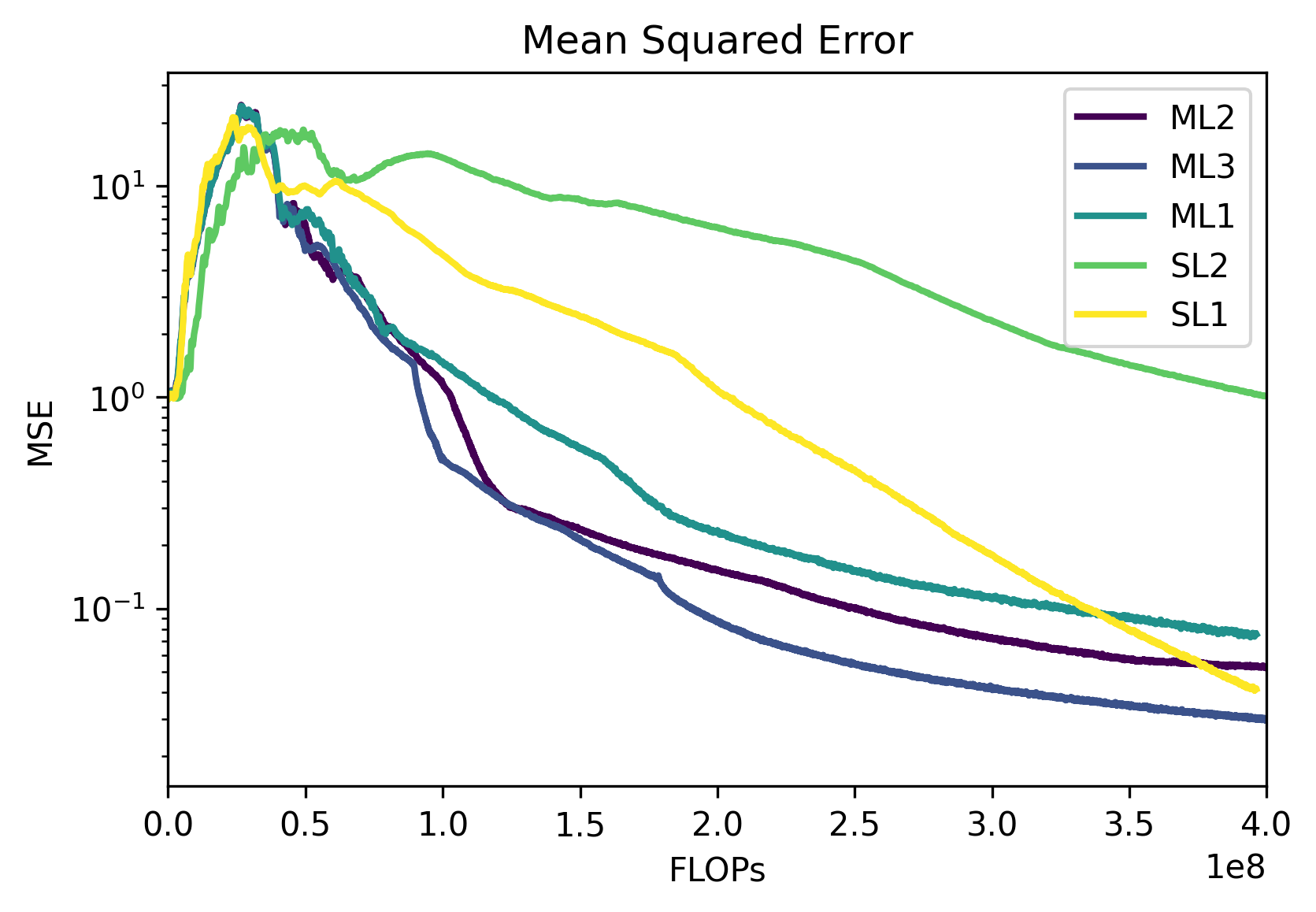
Figure 1: Evolution of the MSE as a function of the computational cost for our different models

Figure 2: Evolution of the loss as a function of the computational cost for our different models

These result may seem encouraging, but this approach remains limited in that it does not overcome a limitation inherent to classical neural network training: high-frequency fitting. This is highlighted in Figure 3 where we test our method on problem (19) with parameters $\alpha=2$ and $\beta=20$.

Figure 3: Results of our method on the Poisson problem (19) for different frequencies. The method indicated as FAML (Frequency-Aware-Multilevel) is the method proposed in the forthcoming Section 5.

An alternative approach is thus warranted, which we develop in the next section.

5 A “frequency-aware” distributed approach

In the hierarchical cases detailed in Section 2, the reduction in computational cost is typically directly proportional to the separation of frequencies. For instance, in multigrid methods, switching to a coarse grid helps to target low frequencies that converge slowly in the fine problem. This does not seem to be the case for neural networks. The F-Principle [45] states that ”deep neural networks often fit target functions from low to high frequencies during the training process”, which is problematic in some cases and seems to affect also MPINNs, leading to a slow convergence, as illustrated at the end of the previous section. The simple alternation of coarse and fine problems doesn’t seem to be sufficient in the context of neural networks.

Several papers have addressed the issue related to the F-Principle by proposing architectures that transform high frequencies of the problem into low frequencies, thereby allowing a more efficient use of the neural networks. Inspired by these papers, we propose a frequency-aware architecture that retains the computational cost savings of multilevel training while incorporating the frequency separation aspect of classical methods.

5.1 A frequency-aware network architecture

Our architecture proposal is mainly inspired by Multi-scale deep neural networks (MscaleDNNs) [24] and WWP [41], which were designed to mitigate the effect of the F-principle in the standard (single level) context. The basic idea is to transform high frequency learning in low frequency learning and to facilitate the separation of the frequency contents of the target function. As a result, these networks show uniform convergence over multiple scales.

The MscaleDNNs architecture achieves this objective thanks to two main ingredients:

• radial scaling in the frequency domain: the first layer is separated into $N$ parts, each receiving a differently scaled input. Several variants of MscaleDNNs have been proposed, we choose to focus here on the most efficient one, which uses parallel sub-networks, each dedicated to a specific input scaling.

• the use of wavelet-inspired and frequency-located activation functions. These functions, with compact support, have good scale separation properties.

WWP networks were proposed by Wang, Wang, and Perdikaris. They use the same principle of input scaling, combined with soft Fourier mapping (SFM):

$$\gamma(z)=s\;\begin{bmatrix}\cos(z)\\ \sin(z)\\ \end{bmatrix}$$

with $s\in[0,1)$ a relaxation parameter.

A ”Fourier features network” was first proposed in [36], which uses a random Fourier features mapping $\gamma$ as a coordinate embedding of the inputs, followed by a conventional fully-connected neural network. This method did mitigate the pathology of spectral bias and helped networks learn high frequencies more effectively. Recent advancements have made it possible to model fully connected neural networks (and thus PINNs) as kernel regression. The authors of [36] suggested that using Fourier mapping affects the width of the kernels and thus the network’s capacity to capture high frequencies. This idea was extended to PINNs in [41] with convincing results, provided that the fixed scalings are too far from the frequencies contained in the solution.

Inspired by their success, we propose here an architecture that combines the positive features of both methods. Our architecture’s output is the sum of several networks that use different scaling vectors, specializing each network for different frequency scales matching the structure presented in our theory in Section 2. To mitigate possible convergence problems arising from a bad choice of the fixed scalings, we have chosen to add learnable weights to the input scaling integers using SFM as a classic activation function.

For low frequency resolution, we choose a classical network using hyperbolic tangent activation functions. For the other networks, we use SFM activation functions for the first layer associated with a scaling from a centred normal distribution whose variance grows with the targeted frequencies. The other layers of the networks use hyperbolic tangent activation functions, thus ensuring our differentiability requirements. We refer to this architecture as Parallel-WWP (P-WWP). Unfortunately, the wavelet-based and frequency-based activation functions utilized in the MSCALE are not continuously differentiable, and thus fail to satisfy our theoretical assumptions. We have however included some (successful) experiments conducted using these functions in Appendix B.

A similar architecture, based on a lower number of subnetworks, has been proposed in [23] for the deep Ritz method [8], which produces a variational solution to problem (16). To the best of our knowledge, this is the first time this architecture has been proposed for PINNs.

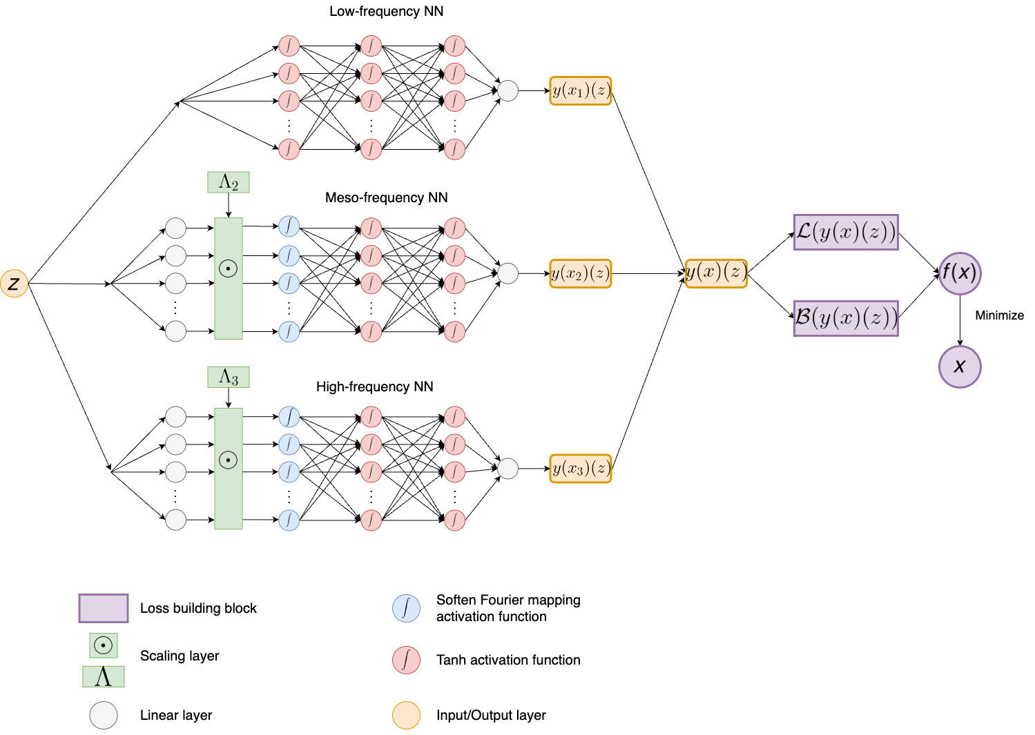
Figure 4: An example of P-WWP architecture

An example of our architecture is illustrated in Figure 4, which consists of three sub-networks, targeting three different frequency ranges defined by their input scaling $\Lambda_{i}$. The lowest frequency network employs $\tanh$ activation functions, while the others use $SFM$ and $\tanh$.

To be effective, this architectures must cover most of the frequencies contained in the a priori unknown PDE’s solution. Therefore, a broad range of frequencies must be covered, employing a large number of neurons, as the target frequencies are defined by the input scalings. As a result, the considerable improvement in accuracy provided by parallel frequency-aware architectures is obtained at the price of a significant increase in the training’s computational cost, making it an ideal candidate for our multilevel approach.

These architectures can be easily incorporated into our framework, where the global network is defined as a sum of $y_{i}$ sub-networks, each responsible for a frequency range defined by its input scaling. Because of this latter characteristics, the resulting approach now belongs to the distributed context discussed in Section 2. In particular, we refer to the combination of the P-WWP network with the ML-BCD algorithm as the FAML (Frequency Aware Multi-Level) method. We use the same selection and termination criteria as in Section 4.2. When several sub-networks are available, the network with the highest ratio $\|g_{i,k}\|/\|g_{k}\|$ is chosen.

5.2 Numerical results

We now illustrate the efficiency of the FAML method on some examples of the form (19) defined in [32]. We first describe the test problems themselves, then specify the considered network architectures and the training setup before describing and commenting the obtained results.

5.2.1 Test problem 1: Circle embedded in a square domain

The domain for the first problem is the square $\Omega=[-1,1]^{2}$ with an embedded circle of radius $R=0.5$ centered at the origin defining $\Omega_{i}$. We consider Neumann boundary conditions on $\Gamma_{i}$ and Dirichlet boundary condition on $\Gamma_{e}$.

The source term and boundary term are given by

$$\left\{\begin{aligned} &r(\rho,\omega)=D(k^{2}-n^{2})\rho^{k-2}\sin(n\omega)\text{ in }\Omega\\ &g(\rho,\omega)=-\frac{Dk}{n}\left(\frac{\rho}{R}\right)^{(n-k)}\rho^{k}\sin(n\omega)+Rq\log\rho\text{ on }\Gamma_{e}\\ &h(\rho,\omega)=1\text{ on }\Gamma_{i}\\ \end{aligned}\right.$$ (20)

where $\rho,\omega$ are the polar coordinates in the plane, $n\in\mathbb{Z}$, $z\in\mathbb{N}$ and $D=(\sqrt{2})^{-\max(k,n)}$. We choose $k=1$ and $n=-5$. The solution is given by $u(\rho,\omega)=-\frac{Dk}{n}\left(\frac{\rho}{R}\right)^{(n-k)}\rho^{k}\sin(n\omega)+R\log\rho$. The solution and the source terms are depicted in Figure 5.

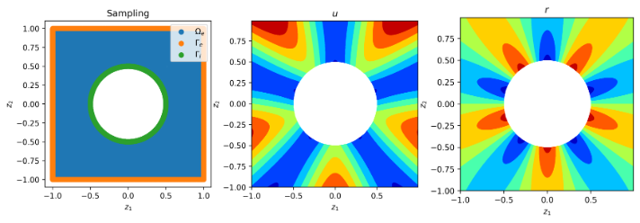
Figure 5: Test problem 1 (cf. (19), (20)). Left: the domain $\Omega$ and its subdomains. Center: the solution $u$. Right: the source term $r$.

Notice the variation in angular frequency as a function of the radius.

5.2.2 Test problem 2: Four-lobe structure

The domain for the second problem is the unit square $\Omega=[0,1]^{2}$ with an embedded surface defined by $\rho(\omega)=R_{m}+R_{d}\cos(4\omega)$ with $R_{m}=0.0305$, $R_{d}=0.117$. We consider Dirichlet boundary conditions for both $\Gamma_{e}$ and $\Gamma_{i}$. The source term and boundary term are given by

$$\left\{\begin{aligned} &r(\rho,\omega)=12(10\rho^{2}-1)e^{-10^{2}}+\sum_{k=1}^{4}40(10r_{k}^{2}-1)\text{ in }\Omega\\ &g(\rho,\omega)=0.3e^{-10\rho^{2}}+\sum_{k=1}^{4}e^{-10r_{k}^{2}}\text{ on }\Gamma_{e}\cup\Gamma_{i}\\ &r_{k}=\sqrt{(x\pm 0.45)^{2}+(y\pm 0.45)^{2}},\;k=1,\dots,4\end{aligned}\right.$$ (21)

where $\rho$ and $\omega$ are the polar coordinates, and $x$ and $y$ the corresponding Cartesian coordinates. The solution is given by $u(\rho,\omega)=0.3e^{-10\rho^{2}}+\sum_{k=1}^{4}e^{-10r_{k}^{2}}$. The solution and the source terms are depicted in Figure 6.

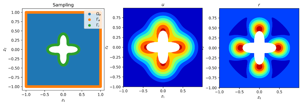
Figure 6: Test problem 2 (cf. (19), (21)). Left: the domain $\Omega$ and its subdomains. Center: the solution $u$. Right: the source term $r$.

5.2.3 Test problem 3: Annulus domain with homogeneous source

We now consider a domain defined by an annulus with inner radius $R_{i}=0.25$ and outer radius $R_{o}=0.75$, and consider a Neumann boundary condition on $\Gamma_{i}$ and a Dirichlet boundary condition on $\Gamma_{e}$. The source term and boundary term are given by

$$\left\{\begin{aligned} &r(\rho,\omega)=0\text{ in }\Omega\\ &g(\rho,\omega)=0\text{ on }\Gamma_{e}\\ &h(\rho,\omega)=1\text{ on }\Gamma_{i}\\ \end{aligned}\right.$$ (22)

where $\rho$ and $\omega$ are the polar coordinates. The solution is given by $u(\rho,\omega)=R_{i}\log(\frac{\rho}{R_{0}})$, which is depicted in Figure 7.

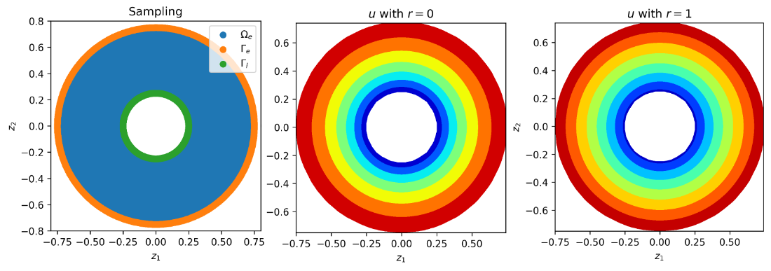
Figure 7: Test problems 3 (cf. (19), (22)) and 4 (cf. (19), (23)). Left: the domain $\Omega$ and its subdomains. Center: the solution $u$ for Test Problem 3. Right: the solution $u$ for Test Problem 4.

5.2.4 Test problem 4: Annulus domain with inhomogeneous source

We finally consider again the domain defined by an annulus with inner radius $R_{i}=0.25$ and the outer radius $R_{o}=0.75$ with Neumann boundary condition on $\Gamma_{i}$ and Dirichlet boundary condition on $\Gamma_{e}$. The source and boundary terms now given by

$$\left\{\begin{aligned} &r(\rho,\omega)=1\text{ in }\Omega\\ &g(\rho,\omega)=0\text{ on }\Gamma_{e}\\ &h(\rho,\omega)=1\text{ on }\Gamma_{i}.\\ \end{aligned}\right.$$ (23)

The solution is then given by $u(\rho,\omega)=\frac{\rho^{2}-R_{0}^{2}}{4}+R_{i}(1-\frac{R_{i}}{2})\log(\frac{\rho}{R_{o}})$.

5.3 Network architectures

We now give the details of the network architectures used in our second set of experiments. It is important to notice that our method is not just applicable to P-WWP networks, but can be used to train any architecture composed of sum of subnetworks.

	input scaling	First Activation	Other Activations
subnetwork 1	None	$\tanh$	$\tanh$
subnetwork 2	$\mathcal{N}(0,20)$	SFM(0.5)	$\tanh$
subnetwork 3	$\mathcal{N}(0,40)$	SFM(0.5)	$\tanh$
subnetwork 4	$\mathcal{N}(0,60)$	SFM(0.5)	$\tanh$

Each of the subnetworks is composed of 3 hidden layers of 100 neurons each. In order to assess computational performance, we also consider the standard single level training applied on the complete network.

5.4 Training setup

We will use the same setup as in Section 4 except for the coefficients $\lambda_{\Omega_{e}}=1,\lambda_{\Gamma_{e}}=100$ and $\lambda_{\Gamma_{i}}=1$ that weight internal and boundary losses.

In order to compare the convergence speeds of the training methods, we decided to consider the computational cost of the training, as the epochs for the two training methods do not have the same cost. For this purpose, we consider as a unit of cost the price of optimising our complete neural network over an epoch. When a subnetwork is selected in the course of the ML-BCD algorithm, the unselected part of the complete network is cached in memory and does not contribute to the subnetwork optimization cost. Since the cost per iteration is linear in the number of parameters when using first-order methods, the cost of optimizing for an epoch one of four subnetworks of identical sizes is $\frac{1}{4}=0.25$ cost units. For these experiments we chose to do 1000 epochs in full network cycle and 4000 epochs in sub-network cycle. Thus the cost of the full and partial training is similar. We do a total of 9 cycles with 1000 epochs on the full network to start the training, for a total computational cost of $1000+9\times(1000+\frac{4000}{4})=19000$ units. For each problem we first compute the curve of the median values over 10 runs of the loss and of the MSE, as a function of epochs and for two different computational budgets (10k and 19k units). We then select the lowest median loss obtained for a given budget and record the associated median MSE.

5.5 Numerical results

Table 2 reports the results just described, obtained with the Frequency-Aware-Multilevel (FAML).

Problem	Budget	MSE	MSE FAML	Loss	Loss FAML
Test pb 1	10000	1.40E-05	2.54E-07	1.64E-01	1.18E-02
	19000	7.70E-06	2.49E-07	6.33E-02	4.89E-03
Test pb 2	10000	1.66E-05	3.99E-07	1.45E-01	1.17E-02
	19000	7.77E-06	2.57E-07	5.38E-02	4.42E-03
Test pb 3	10000	1.05E-05	1.36E-07	1.04E-01	6.76E-03
	19000	3.81E-06	1.11E-07	3.71E-02	2.55E-03
Test pb 4	10000	9.53E-06	1.62E-07	1.02E-01	7.40E-03
	19000	3.58E-06	1.32E-07	3.75E-02	2.63E-03

Table 2: Best median the loss and associated MSE for standard single-level and FAML training (10 independent runs)

In each case, the proposed multi-level training yields lower losses than the standard one. The differences are particularly significant for a small computational budget where the improvement is of several orders of magnitude. The multi-level training also always results in a lower associated MSE.

To provide further insight, we finally provide a typical example allowing the comparison of standard and multi-level training: for Test problem 3, we illustrate in Figure 8 the decrease of the total loss and of its boundary and interior components as well as that of the MSE as a function of computational cost. The multi-level approach clearly outperforms the standard one. (We remind the reader that peaks correspond to the restarts of the optimizer.)

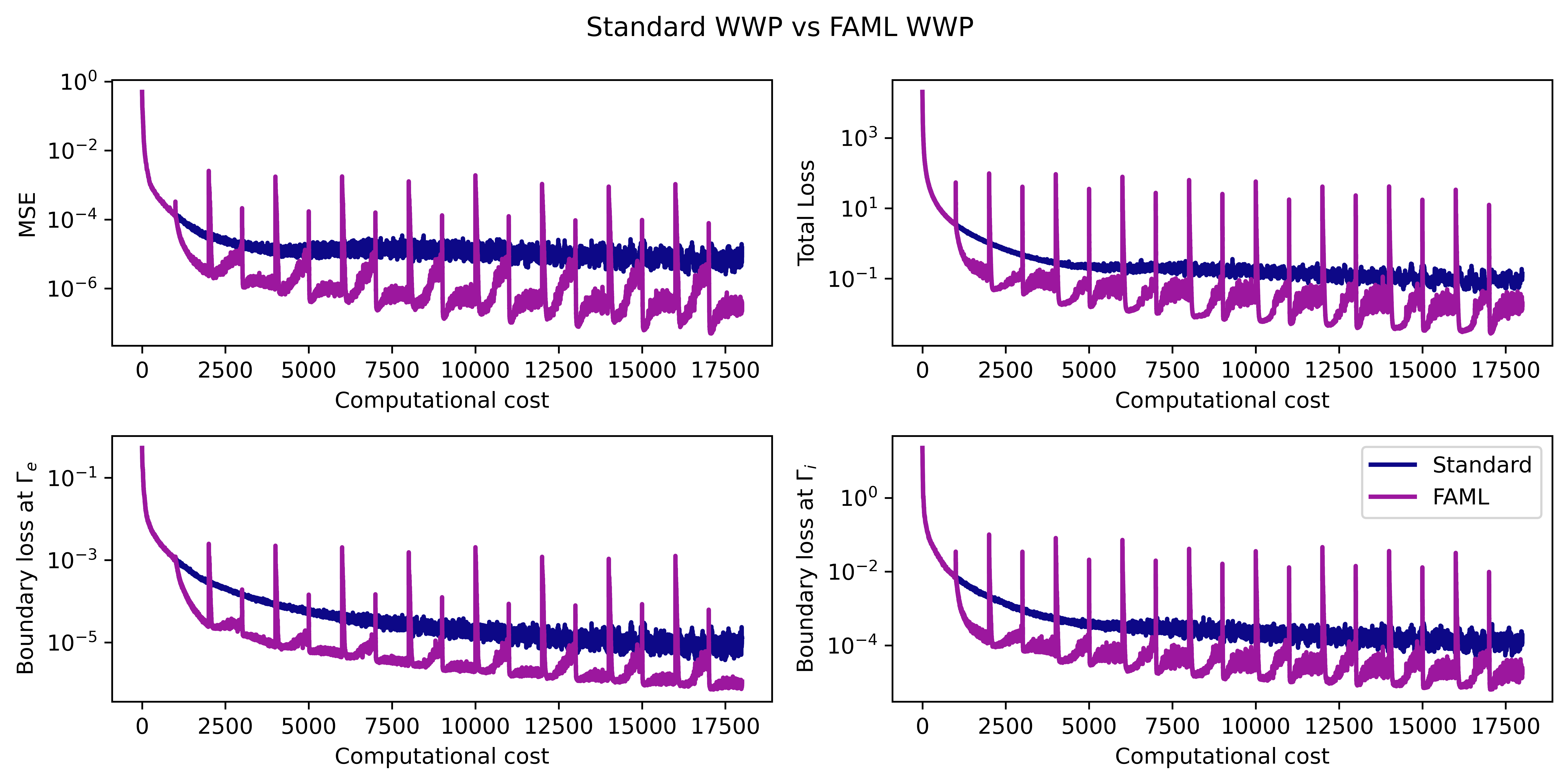
Figure 8: Evolution of MSE and loss values for a typical run on Test problem 3

6 Conclusion and perspectives

We first developed a new point of view on multilevel optimization methods, arguing they can be seen as block-coordinate minimization methods in a higher dimensional space. Distinguishing two contexts (hierarchical and distributed), we reformulated a class of multilevel algorithms in block form and showed how convergence results for block-coordinate methods can be applied to the multilevel case.

We next illustrated this approach for the approximate solution of partial differential equations, using physics-informed neural networks as a block solver, and presented numerical experiments with a method using pure alternating training (in the hierarchical context) and a more elaborate frequency-aware technique (in the distributed one) on complex Poisson problems. On these problems, both resulting multilevel PINNS methods consistently produced lower losses than those obtained using conventionally trained networks. Convergence was also shown to be much faster allowing a considerable reduction of the computational cost to obtain good solutions (often better than those obtained by a classical training).

While these initial results are encouraging, more research remains desirable for a better understanding of the algorithms. Their dependence on techniques to transfer algorithmic hyperparemeters between levels is of particular interest. Applying our approach to more general operator learning is also worth further investigation.

Appendix

Appendix A Proof of Theorem 3.1

Consider applying the ML-BCD algorithm to the minimization of the objective function $f$, which we assume is bounded below by $f_{\rm low}$ and has a Lipschitz continuous gradient (with Lipschitz constant $L$). Let $\alpha<1/L$ be the fixed stepsize used by the algorithm. Consider iteration $k$ and suppose that this iteration occurs in the minimization of subproblem ${\cal A}_{i}$ on the variables given by $x_{i}$. From the Lipschitz continuity of the gradient and (15), we obtain that

$$f(x_{k+1})\leq f(x_{k})-\alpha\nabla_{x}f(x_{k})^{T}\bar{g}_{i,k}+\frac{\alpha^{2}L}{2}\|\bar{g}_{i,k}\|^{2}=f(x_{k})-\alpha\|\bar{g}_{i,k}\|^{2}+\frac{\alpha^{2}L}{2}\|\bar{g}_{i,k}\|^{2}<f(x_{k})-\frac{\alpha}{2}\|\bar{g}_{i,k}\|^{2}.$$

Since the minimization of subproblem ${\cal A}_{i}$ has not yet terminated, we must have that $\|\bar{g}_{i,k}\|=\|g_{i,k}\|\geq\tau\epsilon$, and thus

$$f(x_{k+1})<f(x_{k})-\frac{\alpha\tau^{2}\epsilon^{2}}{2}.$$

Summing this inequality on all iterations, we deduce that, for all $k$ before termination of the ML-BCD algorithm,

$$f(x_{0})-f_{\rm low}\geq f(x_{0})-f(x_{k+1})=\sum_{j=0}^{k}\Big{(}f(x_{j})-f(x_{j+1})\Big{)}\geq\frac{(k+1)\alpha\tau^{2}\epsilon^{2}}{2}.$$

This implies that the algorithm cannot take more than

$$\frac{2(f(x_{0})-f_{\rm low})}{\alpha\tau^{2}\epsilon^{2}}-1$$

iterations before it teminates, proving the theorem with

$$\kappa_{*}=\frac{2(f(x_{0})-f_{\rm low})}{\alpha\tau^{2}}>\frac{2L(f(x_{0})-f_{\rm low})}{\tau^{2}}.$$

$\Box$

Appendix B A Mscale FAML variant and its performance

B.1 Another frequency-aware architecture

This appendix reports on tests conducted using a frequency-aware network architecture based on MscaleDNN defined in [24], instead of the WWP networks used in Section 5. A large part of the success of Mscale networks is due to their wavelet-inspired activation functions. These compactly-supported have good scale separation properties and are constructed so that the bandwidth of their Fourier transform increases with their input scaling. Several activation functions have been proposed in [24], but the most efficient one from a practical point of view has been introduced in [22] and is given by

$$\text{s2ReLU}(z)=\sin(2\pi z)\text{ReLU}(-(z-1))\text{ReLU}(z),$$ (24)

where $z$ is the input scaling. This is a continuous function which decays faster and has better localization property in the frequency domain than the previously proposed sRelu. The amplitude peaks of the differently scaled s2ReLU in the frequency domain are well separated in the Fourier domain. They are indicated by black stars in Figure 9, and we observe their expected monotonic growth with scaling.

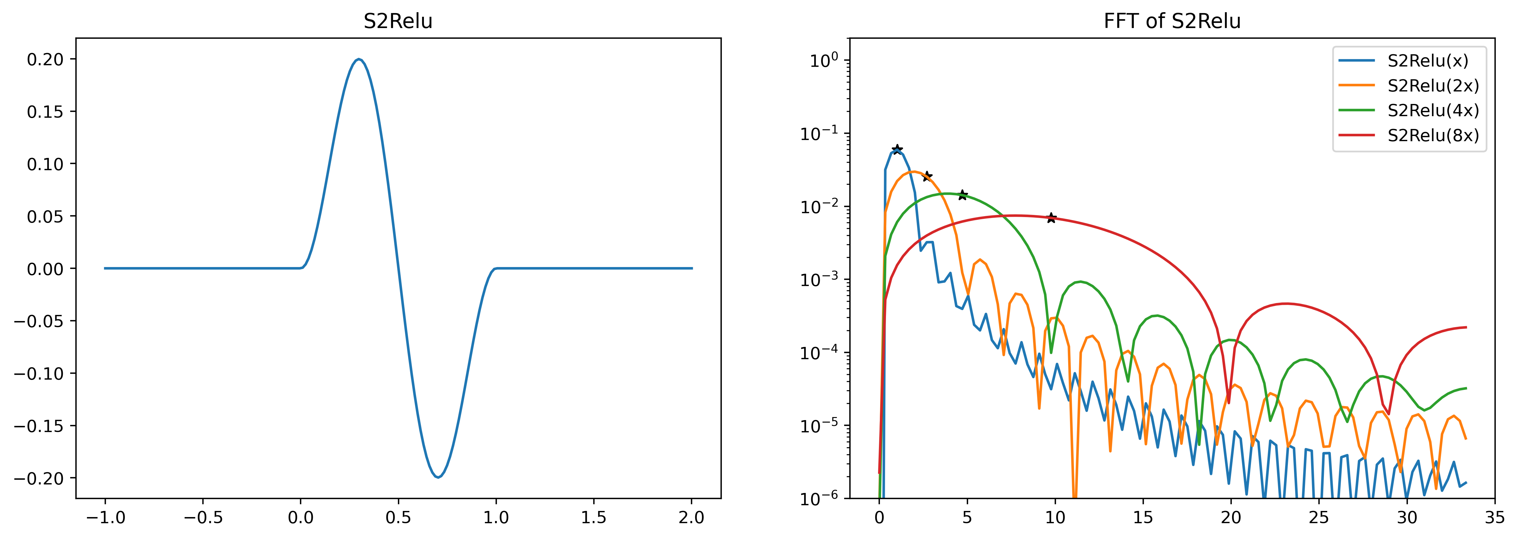
Figure 9: The s2Relu activation function (left) and its Fourier transform for several scalings (right). The black stars highlight the amplitude peaks.

As in Section 5, we use these functions to create a neural network composed of a sum of subnetworks each targeting a different frequency range (analogously to Figure 4). In this modified architecture, the lower frequency networks still use $\tanh$ activation functions while the higher frequency networks now use (24). For each subnetwork, the first activation function is a $SFM$ function associated with a fixed input scaling, as in standard Mscales networks. The details of this architecture are given in Table 3. Each of the subnetworks is composed of 3 hidden layers of 100 neurons each.

	input scaling	First Activation	Other Activations
subnetwork 1	(0.5,1,1.5,…,10)	SFM(1.0)	$\tanh$
subnetwork 2	(11,12,…,29,30)	SFM(0.5)	s2ReLU
subnetwork 3	(31,32,…,50,51)	SFM(0.5)	s2ReLU
subnetwork 4	(51,52,…,69,70)	SFM(0.5)	s2ReLU

Table 3: Details of the parallel Mscale architecture

Associated with the ML-BCD algorithm (exactly as in Section 5), this modified architecture defines an Mscale variant of the FAML approach.

B.2 Numerical results

We tested this approach using the same experimental setup and methodology as that of Section 5 and again compared its performance to that the standard single level training applied on the complete network. The results are reported in Table 4.

Problem	Budget	MSE	MSE FAML	Loss	Loss FAML
Test Pb 1	10000	1.33E-05	2.76E-06	2.49E-01	7.98E-03
	19000	1.85E-06	2.51E-06	4.53E-03	2.50E-03
Test Pb 2	10000	1.22E-05	3.87E-07	1.73E-01	8.14E-04
	19000	6.11E-07	2.74E-08	1.22E-05	3.87E-07
Test Pb 3	10000	1.06E-05	1.85E-07	2.80E-01	1.06E-03
	19000	4.09E-07	1.23E-08	6.17E-04	2.09E-04
Test Pb 4	10000	1.56E-05	1.98E-07	2.84E-01	1.04E-03
	19000	5.24E-07	1.21E-08	6.26E-04	1.85E-04

Table 4: Best median the loss and associated MSE for standard single-level and Mscale-FAML training (10 independent runs)

As was the case when using P-WWP networks, the Mscale FAML variant produced lower losses than the standard training in each case. The differences are particularly significant for a small computational budget where the improvement is of several orders of magnitude. This is also almost always the case for the associated MSE. These results thus remain excellent, despite the fact that our complexity theory does not formally cover the Mscale FAML variant because of the non-smoothness of (24).

References

- [1] V. S. Amaral, R. Andreani, E. G. Birgin, D. S. Marcondes, and J. M. Martínez. On complexity and convergence of high-order coordinate descent algorithms for smooth nonconvex box-constrained minimization. Journal of Global Optimization, 84(3):527–561, 2022.
- [2] A. Borzi and K. Kunisch. A globalisation strategy for the multigrid solution of elliptic optimal control problems. Optimization Methods and Software, 21(3):445–459, 2006.
- [3] W. L. Briggs, V. E. Henson, and S. F. McCormick. A Multigrid Tutorial. SIAM, Philadelphia, USA, 2nd edition, 2000.
- [4] S. Cai, Z. Mao, Z. Wang, M. Yin, and G. E. Karniadakis. Physics-informed neural networks (PINNs) for fluid mechanics: A review. Acta Mechanica Sinica, 37(12):1727–1738, 2021.
- [5] H. Calandra, S. Gratton, E. Riccietti, and X. Vasseur. On high-order multilevel optimization strategies. SIAM Journal on Optimization, 31(1):307–330, 2021.
- [6] C. Cartis, N. I. M. Gould, and Ph. L. Toint. Evaluation complexity of algorithms for nonconvex optimization. Number 30 in MOS-SIAM Series on Optimization. SIAM, Philadelphia, USA, June 2022.
- [7] J. Chung, S. Ahn, and Y. Bengio. Hierarchical multiscale recurrent neural networks. arXiv:1609.01704, 2016.
- [8] B. Yu et al. The deep Ritz method: a deep learning-based numerical algorithm for solving variational problems. Communications in Mathematics and Statistics, 6:1–12, 2018.
- [9] G. Farhani, A. Kazachek, and B. Wang. Momentum diminishes the effect of spectral bias in physics-informed neural networks. arXiv:2206.14862, 2022.
- [10] A. A. Goldstein. Optimization of Lipschitz continuous functions. Mathematical Programming, Series A, 13(1):14–22, 1977.
- [11] S. Gratton, A. Sartenaer, and Ph. L. Toint. On recursive multiscale trust-region algorithms for unconstrained minimization. In F. Jarre, C. Lemaréchal, and J. Zowe, editors, Oberwolfach Reports: Optimization and Applications, 2005.
- [12] S. Gratton, A. Sartenaer, and Ph. L. Toint. Second-order convergence properties of trust-region methods using incomplete curvature information, with an application to multigrid optimization. Journal of Computational and Applied Mathematics, 24(6):676–692, 2006.
- [13] S. Gratton, A. Sartenaer, and Ph. L. Toint. Recursive trust-region methods for multiscale nonlinear optimization. SIAM Journal on Optimization, 19(1):414–444, 2008.
- [14] Ch. Gross and R. Krause. On the globalization of ASPIN employing trust-region control strategies - convergence analysis and numerical examples. Technical Report 2011-03, Universita della Svizzera italiana, Lugano, CH, 2011.
- [15] E. Haber and L. Ruthotto. Stable architectures for deep neural networks. Inverse Problems, 34(1):014004, 2017.
- [16] E. Haber, L. Ruthotto, E. Holtham, and S.-H. Jun. Learning across scales—multiscale methods for convolution neural networks. In Thirty-Second AAAI Conference on Artificial Intelligence, pages 3142–3148, 2018.
- [17] W. Hackbusch. Multi-grid Methods and Applications. Number 4 in Springer Series in Computational Mathematics. Springer Verlag, Heidelberg, Berlin, New York, 1995.
- [18] M. I. Jordan, T. Lin, and M. Zampetakis. On the complexity of deterministic nonsmooth and nonconvex optimization. arXiv:2209.12403, 2022.
- [19] D. Kingma and J. Ba. Adam: A method for stochastic optimization. In Proceedings in the International Conference on Learning Representations (ICLR), 2015.
- [20] S. Kong and A. Lewis. The cost of nonconvexity in nonconvex nonsmooth optimization. arXiv:2210.00652, 2022.
- [21] A. Kopaničáková and R. Krause. Globally convergent multilevel training of deep residual networks. SIAM Journal on Scientific Computing, 0:S254–S280, 2022.
- [22] X.-A. Li. A multi-scale DNN algorithm for nonlinear elliptic equations with multiple scales. Communications in Computational Physics, 28(5):1886–1906, 2020.
- [23] X.-A. Li, Z.-Q. J. Xu, and L. Zhang. Subspace decomposition based DNN algorithm for elliptic type multi-scale PDEs. arXiv:2112.06660, 2021.
- [24] Z. Liu, W. Cai, and Z.-Q. J. Xu. Multi-scale deep neural network (MscaleDNN) for solving Poisson-Boltzmann equation in complex domains. Communications in Computational Physics, 28(5):1970–2001, 2020.
- [25] P. Perdikaris M. Raissi and G. E. Karniadakis. Physics-informed neural networks: A deep learning framework for solving forward and inverse problems involving nonlinear partial differential equations. Journal of Computational Physics, 378:686–707, 2019.
- [26] S. Mishra and R. Molinaro. Estimates on the generalization error of physics-informed neural networks for approximating a class of inverse problems for PDEs. IMA Journal of Numerical Analysis, 42:981–1022, 2022.
- [27] S. G. Nash. A multigrid approach to discretized optimization problems. Optimization Methods and Software, 14:99–116, 2000.
- [28] Y. Nesterov. Introductory Lectures on Convex Optimization. Applied Optimization. Kluwer Academic Publishers, Dordrecht, The Netherlands, 2004.
- [29] Y. Nesterov. Efficiency of coordinate descent methods for huge-scale optimization problems. SIAM Journal on Optimization, 22:341–362, 2012.
- [30] M. J. D. Powell. On search directions for minimization algorithms. Mathematical Programming, 4:193–201, 1973.
- [31] N. Rahaman, A. Baratin, D. Arpit, F. Draxler, M. Lin, F. Hamprecht, Y. Bengio, and A. Courville. On the spectral bias of neural networks. In International Conference On Machine Learning, pages 5301–5310, 2019.
- [32] N. R. Rapaka and R. Samtaney. An efficient Poisson solver for complex embedded boundary domains using the multi-grid and fast multipole methods. Journal of Computational Physics, 410:109387, 2020.
- [33] Peter Richtárik and Martin Takáč. Iteration complexity of randomized block-coordinate descent methods for minimizing a composite function. Mathematical Programming, 144(1-2):1–38, 2014.
- [34] B. Ronen, D. Jacobs, Y. Kasten, and S. Kritchman. The convergence rate of neural networks for learned functions of different frequencies. Proceedings of the 33rd International Conference on Neural Information Processing Systems, page 4761–4771, 2019.
- [35] Y. Shin. On the convergence of physics informed neural networks for linear second-order elliptic and parabolic type PDEs. Communications in Computational Physics, 28(5):2042–2074, 2020.
- [36] Matthew Tancik, Pratul Srinivasan, Ben Mildenhall, Sara Fridovich-Keil, Nithin Raghavan, Utkarsh Singhal, Ravi Ramamoorthi, Jonathan Barron, and Ren Ng. Fourier features let networks learn high frequency functions in low dimensional domains. Advances in Neural Information Processing Systems, 33:7537–7547, 2020.
- [37] L. Tian and A. Man-Cho So. Computing Goldstein -stationary points of Lipschitz functions in iterations via random conic perturbation. arXiv:2112.09002, 2021.
- [38] U. Trottenberg, C. W. Oosterlee, and A. Schüller. Multigrid. Elsevier, Amsterdam, The Netherlands, 2001.
- [39] K. Tsung-Wei, M. Maire, and S. X. Yu. Multigrid neural architectures. In Proceedings of the IEEE Conference on Computer Vision and Pattern Recognition, pages 6665–6673, 2017.
- [40] C. von Planta, A. Kopaničáková, and R. Krause. Training of deep residual networks with stochastic MG/OPT. arXiv 2108.04052, 2021.
- [41] S. Wang, H. Wang, and P. Perdikaris. On the eigenvector bias of Fourier feature networks: From regression to solving multi-scale PDEs with physics-informed neural networks. Computer Methods in Applied Mechanics and Engineering, 384:113938, 2021.
- [42] Sifan Wang, Xinling Yu, and Paris Perdikaris. When and why pinns fail to train: A neural tangent kernel perspective. Journal of Computational Physics, 449:110768, 2022.
- [43] S. J. Wright. Coordinate descent algorithms. Mathematical Programming, Series A, 151(1):3–34, 2015.
- [44] C.-Y. Wu, R. Girshick, K. He, Ch. Feichtenhofer, and Ph. Krahenbuhl. A multigrid method for efficiently training video models. In Proceedings of the IEEE/CVF Conference on Computer Vision and Pattern Recognition, pages 153–162, 2020.
- [45] Z.-Q. J. Xu. Frequency principle: Fourier analysis sheds light on deep neural networks. Communications in Computational Physics, 28(5):1746–1767, 2020.
- [46] J. Zhang, H. Lin, S. Jegelka, S. Sra, and A. Jadbabaie. Complexity of finding stationary points of nonconvex nonsmooth functions. In Proceedings of the 37th International Conference on Machine Learning, PMLR, volume 119, pages 11173–11182, 2020.