Engineering Rank/Select Data Structures for Big-Alphabet Strings

Abstract

Big-alphabet strings are common in several scenarios such as information retrieval and natural-language processing. The efficient storage and processing of such strings usually introduces several challenges that are not witnessed in smaller-alphabets strings. This paper studies the efficient implementation of one of the most effective approaches for dealing with big-alphabet strings, namely the alphabet-partitioning approach. The main contribution is a compressed data structure that supports the fundamental operations $\mathsf{rank}$ and $\mathsf{select}$ efficiently. We show experimental results that indicate that our implementation outperforms the current realizations of the alphabet-partitioning approach. In particular, the time for operation $\mathsf{select}$ can be improved by about 80%, using only 11% more space than current alphabet-partitioning schemes. We also show the impact of our data structure on several applications, like the intersection of inverted lists (where improvements of up to 60% are achieved, using only 2% of extra space), the representation of run-length compressed strings, and the distributed-computation processing of $\mathsf{rank}$ and $\mathsf{select}$ operations.

1 Introduction

Strings are a fundamental data type in computer science. Today they are intensively used in applications such as text, biological, and source code databases, hence their efficient manipulation is key. By efficiency we mean being able to (1) use as less space as possible to store them, and (2) manipulate them efficiently, supporting operations of interest.

Let $s[1..n]$ be a string of length $n$, with symbols drawn over an alphabet $\Sigma=\{0,\ldots,\sigma-1\}$. We define the following operations on strings that will be studied in this paper:

• $s.\mathsf{rank}_{c}(i)$: for $1\leq i\leq n$ and symbol $c\in\Sigma$, yields the number of occurrences of $c$ in $s[1..i]$.

• $s.\mathsf{select}_{c}(j)$: for $c\in\Sigma$ and $1\leq j\leq n_{c}$, yields the position of the $j$-th occurrence of symbol $c$ in $s$. Here, $n_{c}=s.\mathsf{rank}_{c}(n)$ is the total number of occurrences of $c$ in $s$.

• $s.\mathsf{access}(i)$: yields symbol $s[i]$, for $1\leq i\leq n$.

These operations are fundamental for many applications [46], such as snippet extraction in text databases [6], query processing in information retrieval [4, 3], and the space-efficient representation of cardinal trees, text-search data structures, and graphs [13], among others. As the amount of data managed by these applications is usually large, space-efficient data structures that support these operations are fundamental [46]. Succinct data structures use space close to the information-theory minimum, while supporting operations efficiently. Compressed data structures, on the other hand, take advantage of certain regularities in the data to further reduce the space usage. The main motivation behind the use of space-efficient data structures is the in-memory processing of big amounts of data, avoiding expensive secondary-memory accesses and saving important time.

Starting with the seminal work by Jacobson [37], space-efficient data structures have been one of the main lines in data-structure research [5]. After around 35 years, this is a mature research area with most fundamental theoretical problems already solved. Thus, research has slightly turned into the applications of space-efficient data structures and technology transfer. Being able to properly implement the theoretical proposals is not trivial [46], usually requiring in-depth studies and strong algorithm engineering. The main focus of this paper is the engineering of space-efficient data structures supporting $\mathsf{rank}$ and $\mathsf{select}$ operations on strings. In particular, we are interested in big-alphabet strings, which are common in scenarios like information retrieval and natural language processing and introduce additional challenges when implementing them. To illustrate this, the most relevant data structures supporting $\mathsf{rank}$ and $\mathsf{select}$ operations on strings are wavelet trees [35], using $n\lg{\sigma}(1+o(1))+\Theta(\sigma w)$, where $w=\Omega(\lg{n})$ is the word size (in bits) of the word-RAM model we assume in this paper. For big $\sigma$, the $\Theta(\sigma w)$ term dominates the space usage. Wavelet matrices [24] tackle this linear alphabet dependency using just $n\lg{\sigma}(1+o(1))$ bits of space, while supporting $\mathsf{rank}$, $\mathsf{select}$, and $\mathsf{access}$ in $O\!\left(\lg{\sigma}\right)$ time. However, they have two main drawbacks:

1. The $O\!\left(\lg{\sigma}\right)$ computation time of the operations can be high in practice, as wavelet matrices are implemented as a bit string on which $\lceil\lg{\sigma}\rceil$ $\mathsf{rank}$ or $\mathsf{select}$ operations are needed to support the corresponding $\mathsf{rank}$ and $\mathsf{select}$ on $s$. Operation $\mathsf{rank}$ on bit strings is typically supported in $\sim$25–50 nanoseconds using the most efficient data structures from the sdsl library [31], whereas $\mathsf{select}$ on a bit string typically takes $\sim$100–300 nanoseconds. On a big-alphabet string, $\lceil\lg{\sigma}\rceil$ can be high, hence the total operation time can become impractical. For instance, for the well-known GOV2 collection [23], $\lceil\lg{\sigma}\rceil=25$, whereas for ClueWeb [1] we have $\lceil\lg{\sigma}\rceil=26$.

2. Although they use only $o(n\lg{\sigma})$ additional bits on top of the plain representation of string $s$, no compression is achieved. In practice, strings have regularities that could be used to improve the space usage, using space proportional to some compressibility measure (such as, e.g., the empirical entropy of the string [41]).

The approach by Golynski et al. [32] improves the operation times to $O\!\left(\lg\lg{\sigma}\right)$ (and $\mathsf{select}$ to $O\!\left(1\right)$ time), improving practical performance notoriously compared to wavelet matrices, yet still using non-compressed space. The alphabet-partitioning approach by Barbay et al. [13], on the other hand, keeps the same computation times as Golynsky et al.’s approach, yet using compressed space —so, avoiding both drawbacks mentioned above. The main disadvantage is, however, that the theoretical times obtained by Barbay et al. [13] rely on the multi-ary wavelet trees by Ferragina et al. [26] which have been shown impractical by Bowe [17, 46]. Indeed, the experiments in this paper indicate that alphabet partitioning and wavelet matrices have similar operation times, although the former uses less space.

Contributions

In this paper we study practical ways to implement the alphabet-partitioning approach [13]. Our main contributions are as follows:

1. We carry out algorithm engineering on the alphabet-partition approach by Barbay et al. [13], obtaining an implementation that uses compressed space while supporting operations $\mathsf{rank}$ and $\mathsf{select}$ efficiently.

2. We show that our approach yields competitive trade-offs when used for (i) snippet extraction from text databases and (ii) intersection of inverted lists. Both operations are of major interest for modern information retrieval systems.

3. Similar as how Barbay et al. [13] showed that alphabet partitioning eases zero-order compression, we show it can also improve run-length compression of big-alphabet strings formed by $r$ sufficiently-long runs. We introduce a competitive alternative both in theory and practice (see Table 2 on page 2).

4. We carry out intensive algorithm engineering to implement our above run-length compression approach. In particular, we implement and try several data structures to represent bit strings with runs of 0s and 1s, in order to use the most effective alternatives as building blocks of our data structure.

5. We show that our approach can be efficiently implemented on a distributed-memory system.

An overall conclusion from our study is that our implementation of alphabet partitioning is not only effective (and efficient) to support the fundamental $\mathsf{rank}$ and $\mathsf{select}$ operations, but also to support several operations that are key for implementing modern information retrieval systems [19, 20].

2 Related Work

The main problem we deal with in this paper is that of supporting operations $\mathsf{rank}$ and $\mathsf{select}$ efficiently on strings. We review in this section the main concepts and solutions for the problem.

2.1 Succinct Data Structures for Bit Vectors

Given a bit vector $B[1..n]$ with $m$ 1 bits, operations $\mathsf{rank}$ and $\mathsf{select}$ can be generalized as $\mathsf{rank}_{b}$ and $\mathsf{select}_{b}$, for $b\in\{\texttt{0},\texttt{1}\}$. The following space-efficient data structures offer the most interesting trade-offs:

• The SDarray data structure by Okanohara and Sadakane [47] uses $m\lg{\frac{n}{m}}+2m+o(m)$ bits of space, and supports $\mathsf{select}$ in $O(1)$ time (provided we replace the $\mathsf{rank}$/$\mathsf{select}$ bit vector data structure on which SDarray is based by a constant-time $\mathsf{select}$ data structure [43]). Operations $\mathsf{rank}$ and $\mathsf{access}$ are supported in $O\left(\lg{\frac{n}{m}}\right)$ time.

• The data structure by Raman et al. [50] uses $\lg{n\choose m}+O\!\left(n/\lg^{2}{n}\right)$ bits of space, supporting $\mathsf{rank}$, $\mathsf{select}$, and $\mathsf{access}$ in $O\!\left(1\right)$ time.

• The data structure by Pǎtraşcu [49] improves the second term in the space usagevof the above data structure, requiring $\lg{n\choose m}+O\!\left(n/\lg^{c}{(n/c)}\right)+O\!\left(n^{3/4}\mathrm{polylog}(n)\right)$ bits of space, for any $c>0$, while supporting all operations in $O\!\left(1\right)$ time.

2.2 Compressed Data Structures

A compressed data structure uses space proportional to some compression measure of the data, e.g., the $0$-th order empirical entropy of a string $s[1..n]$ over an alphabet of size $\sigma$, which is denoted by $H_{0}(s)$ and defined as:

$$H_{0}(s)=\sum_{c\in\Sigma}{\frac{n_{c}}{n}\lg{\frac{n}{n_{c}}}},$$ (1)

where $n_{c}$ is the number of occurrences of symbol $c$ in $s$. The sum includes only those symbols $c$ that do occur in $s$, so that $n_{c}>0$. The value $H_{0}(s)\leq\lg{\sigma}$ is the average number of bits needed to encode each string symbol, provided we encode them using $\lg{\frac{n}{n_{c}}}$ bits.

We can generalize this definition to that of $H_{k}(s)$, the $k$-th order empirical entropy of string $s$, for $k>0$, defined as

$$H_{k}(s)=\sum_{a\in\Sigma^{k}}{\frac{|s_{a}|}{n}H_{0}(s_{a})},$$ (2)

where $s_{a}$ denotes the string of symbols obtained from concatenating all symbols of $s$ that are preceded by a given context $a$ of length $k$. It holds that $0\leq H_{k}(s)\leq\ldots\leq H_{1}(s)\leq H_{0}(s)\leq\lg{\sigma}$, for any $k$.

Following Belazzougui and Navarro [15], in general we call succinct a string representation that uses $n\lg{\sigma}+o(n\lg{\sigma})$ bits, zeroth-order compressed a data structure that uses $nH_{0}(s)+o(n\lg{\sigma})$ bits, and high-order compressed one using $nH_{k}(s)+o(n\lg{\sigma})$ bits. We call fully-compressed a compressed data structure such that the redundancy is also compressed, e.g., to use $nH_{0}(s)(1+o(1))$ bits.

2.3 Rank/Select Data Structures on Strings

Let $s[1{..}n]$ be a string of length $n$ with symbols drawn from an alphabet $\Sigma=\{0,\ldots,\sigma-1\}$. We review next the state-of-the-art approaches for supporting $\mathsf{rank}$ and $\mathsf{select}$ on $s$. Table 1 summarizes the space/time trade-offs of the approaches we will discuss next.

Table 1: Space/time trade-offs for supporting operations $\mathsf{rank}$, $\mathsf{select}$, and $\mathsf{access}$ on a string $s[1{..}n]$ of symbols drawn from an alphabet of size $\sigma$.

Authors	Space (bits)	$\mathsf{access}$	$\mathsf{rank}$	$\mathsf{select}$
[35]	$n\lg{\sigma}+o(n\lg{\sigma})+\Theta(\sigma w)$	$O\!\left(\lg{\sigma}\right)$	$O\!\left(\lg{\sigma}\right)$	$O\!\left(\lg{\sigma}\right)$
[26], [33]	$n(H_{0}(s)+o(1))+\Theta(\sigma w)$	$O\!\left(1+\frac{\lg{\sigma}}{\lg\lg{n}}\right)$	$O\!\left(1+\frac{\lg{\sigma}}{\lg\lg{n}}\right)$	$O\!\left(1+\frac{\lg{\sigma}}{\lg\lg{n}}\right)$
[24]	$n\lg{\sigma}+o(n\lg{\sigma})$	$O\!\left(\lg{\sigma}\right)$	$O\!\left(\lg{\sigma}\right)$	$O\!\left(\lg{\sigma}\right)$
[32]	$n\lg{\sigma}+n\cdot o(\lg{\sigma})$	$O\!\left(\lg{\lg{\sigma}}\right)$	$O\!\left(\lg\lg{\sigma}\right)$	$O\!\left(1\right)$
[36]	$nH_{k}(s)+O\!\left(\frac{n\lg{\sigma}}{\lg\lg{\sigma}}\right)$ (†)	$O\!\left(1\right)$	$O\!\left(\lg\lg{\sigma}\right)$	$O\!\left(\lg{\lg{\sigma}}\right)$
[13]	$nH_{0}(s)(1+o(1))+o(n)$	$O\!\left(\lg\lg{\sigma}\right)$	$O\!\left(\lg\lg{\sigma}\right)$	$O\!\left(1\right)$
[15]	$n(H_{0}(s)+o(1))$	$O\!\left(1+\frac{\lg{\sigma}}{\lg{w}}\right)$	$O\!\left(1+\frac{\lg{\sigma}}{\lg{w}}\right)$	$O\!\left(1+\frac{\lg{\sigma}}{\lg{w}}\right)$
	$nH_{0}(s)(1+o(1))+o(n)$	$O\!\left(1\right)$	$O\!\left(\lg{\frac{\lg{\sigma}}{\lg{w}}}\right)$	any $\omega(1)$
	$nH_{k}(s)+O\!\left(n\lg\lg{\sigma}\right)$ (‡)	$O\!\left(1\right)$	$O\!\left(\lg{\frac{\lg{\sigma}}{\lg{w}}}\right)$	any $\omega(1)$
This paper	$nH_{0}(s)(1+o(1))+o(n)$	$O\!\left(\max\{\lg^{2}{(n)},L\}\right)$ $(\sharp)$	$O\!\left(\lg\lg{\sigma}\right)$	$O\!\left(1\right)$

(†): for any $k=o(\frac{\lg_{\sigma}{n}}{\lg\lg{\sigma}})$.
(‡): for any $k=o(\lg_{\sigma}{n})$, and $\lg{\sigma}=\omega(\lg{w})$.
$(\sharp)$: time for accessing $L\geq 1$ consecutive symbols.

2.3.1 Wavelet Trees

A wavelet tree [35] (WT for short) is a succinct data structure that supports operations $\mathsf{rank}$ and $\mathsf{select}$ on the input string $s$, among many other operations (see, e.g., the work by Navarro [45]). The space requirement is $n\lg{\sigma}+o(n\lg{\sigma})+\Theta(\sigma w)$ bits [35], supporting operations $\mathsf{rank}$, $\mathsf{select}$, and $\mathsf{access}$ take $O(\lg{\sigma})$ time. Term $\Theta(\sigma w)$ in the space usage corresponds to the number of pointers needed to represent the $\Theta(\sigma)$-node binary tree on which a WT is built. This space is negligible only for small alphabets, becoming dominant for big alphabets, e.g., $\sigma=\sqrt{n}$ or extreme cases like $\sigma=O\!\left(n\right)$. There are practical scenarios where big alphabets are common, such as the representation of labeled graphs to support join operations on them [7].

To achieve compressed space, the WT can be given the shape of the Huffman tree, obtaining $nH_{0}(s)(1+o(1))+O\!\left(n\right)+\Theta(\sigma w)$ bits of space. Operations take $O(\lg{n})$ worst-case, and $O\!\left(1+H_{0}(s)\right)$ time on average [46]. Alternatively, one can use compressed bit vectors [50] to represent each WT node. The space usage in that case is $nH_{0}(s)+o(n\lg{\sigma})+\ \Theta(\sigma w)$ bits, whereas operations take $O(\lg{\sigma})$ time. Notice that even though one is able to compress the main components of the WT, the term $\Theta(\sigma w)$ keeps uncompressed and hence is problematic for big alphabets.

The approach by Ferragina et al. [26], which is based on multiary WTs, supports operations in $O(1+\frac{\lg{\sigma}}{\lg\lg{n}})$ worst-case time, and the space usage is $nH_{0}(S)+o(n\lg{\sigma})+\Theta(\sigma w)$ bits. Later, Golynski et al. [33] improved the (lower-order term of the) space usage to $nH_{0}(s)+o(n)+\Theta(\sigma w)$ bits. Notice that if $\sigma=O\!\left(\textrm{polylog}(n)\right)$, these approaches allow one to compute operations in $O\!\left(1\right)$ time.

To avoid the $\Theta(\sigma w)$ term in the space usage of WTs, wavelet matrices [24] (WM, for short) concatenate the $\Theta(\sigma)$ WT nodes into a single bit vector. These nodes are arranged in such a way that the pointers between nodes can be simulated using operations $\mathsf{rank}$ (to go down to a child node) and $\mathsf{select}$ (to go up to a parent node) on the bit vector that implements the WM. Thus, operation $\mathsf{rank}$ and $\mathsf{select}$ on the input string $s$ are still supported in $O\!\left(\lg{\sigma}\right)$ time provided $\mathsf{rank}$ and $\mathsf{select}$ are supported in $O\!\left(1\right)$ time on the underlying bit vector. However, even though both accessing a pointer and operations $\mathsf{rank}$/$\mathsf{select}$ take constant time, the latter has a bigger constant and hence is slower in practice. The space usage is $n\lg{\sigma}+o(n\lg{\sigma})$ bits, avoiding the alphabet-unfriendly term. As WM basically implement a WT avoiding the space of pointers, they are able to support also all operations a WT can support [45].

2.3.2 Reducing to Permutations and Further Improvements

Golynski et al. [32] introduce an approach based on data structures for representing permutations (and their inverses) [44]. The resulting data structure is more effective for larger alphabet than the above WTs schemes (including WM). Their solution uses $n\lg{\sigma}+n\cdot o(\lg{\sigma})$ bits of space, supporting operation $\mathsf{rank}$ in $O\!\left(\lg\lg{\sigma}\right)$ time, and operations $\mathsf{select}$ and $\mathsf{access}$ in $O\!\left(1\right)$ time (among other trade-offs, see the original paper for details). Later, Grossi et al. [36] improved the space usage achieving high-order compression, that is, $nH_{k}(s)+O\!\left(\frac{n\lg{\sigma}}{\lg\lg{\sigma}}\right)$ bits. Operations $\mathsf{rank}$ and $\mathsf{select}$ are supported in $O\!\left(\lg\lg{\sigma}\right)$, whereas $\mathsf{access}$ is supported in $O\!\left(1\right)$ time.

2.3.3 Alphabet Partitioning

We are particularly interested in this paper in the alphabet-partitioning approach [13]. Given an alphabet $\Sigma=\{0,\ldots,\sigma-1\}$, the aim of alphabet partitioning is to divide $\Sigma$ into $p$ sub-alphabets $\Sigma_{0},\Sigma_{1},\ldots,\Sigma_{p-1}$, such that $\bigcup_{i=0}^{p-1}{\Sigma_{i}}=\Sigma$, and $\Sigma_{i}\cap\Sigma_{j}=\emptyset$ for all $i\not=j$.

The Mapping from Alphabet to Sub-alphabet

The data structure [13] consists of an alphabet mapping $m[1..\sigma]$ such that $m[i]=j$ iff symbol $i\in\Sigma$ has been mapped to sub-alphabet $\Sigma_{j}$. Within $\Sigma_{j}$, symbols are re-enumerated from 0 to $|\Sigma_{j}|-1$ as follows: if there are $k$ symbols smaller than $i$ that have been mapped to $\Sigma_{j}$, then $i$ is encoded as $k$ in $\Sigma_{j}$. Formally, $k=m.\mathsf{rank}_{j}(i)$. Let $n_{j}=|\{i,~{}~{}m[s[i]]=j\}|$ be the number of symbols of string $s$ that have been mapped to sub-alphabet $\Sigma_{j}$. A way of defining the partitioning (which is called sparse [13]) is:

$$m[\alpha]=\left\lceil\lg{\left(\frac{n}{n_{\alpha}}\right)}\lg{n}\right\rceil,$$ (3)

where symbol $\alpha\in\Sigma$ occurs $n_{\alpha}$ times in $s$. Notice that $m[\alpha]\leq\lceil\lg^{2}{n}\rceil$.

The Sub-alphabet Strings

For each sub-alphabet $\Sigma_{\ell}$, we store the subsequence $s_{\ell}[1..n_{\ell}]$, $\ell=1,\ldots,p$, with the symbols of the original string $s$ that have been mapped to sub-alphabet $\Sigma_{\ell}$.

The Mapping from String Symbols to Sub-alphabets

In order to retain the original string, we store a sequence $t[1..n]$, which maps every symbol $s[i]$ into the corresponding sub-alphabet. That is, $t[i]=m[s[i]]$. If $\ell=t[i]$, then the corresponding symbol $s[i]$ has been mapped to sub-alphabet $\Sigma_{\ell}$, and has been stored at position $t.\mathsf{rank}_{\ell}(i)$ in $s_{\ell}$. Also, symbol $s[i]$ in $\Sigma$ corresponds to symbol $m.\mathsf{rank}_{\ell}(s[i])$ in $\Sigma_{\ell}$. Thus, we have $s_{\ell}[t.\mathsf{rank}_{\ell}(i)]=m.\mathsf{rank}_{\ell}(s[i])$.

$$s=\mathtt{alabar\_a\_la\_alabarda}$$

$$\Sigma_{1}=\{\mathtt{a}\};~{}~{}~{}\Sigma_{2}=\{\mathtt{l},\mathtt{\_}\};~{}~{}~{}\Sigma_{3}=\{\mathtt{b},\mathtt{r}\};~{}~{}~{}\Sigma_{4}=\{\mathtt{d}\}$$

$$t=1~{}~{}2~{}~{}1~{}~{}3~{}~{}1~{}~{}3~{}~{}2~{}~{}1~{}~{}2~{}~{}2~{}~{}1~{}~{}2~{}~{}1~{}~{}2~{}~{}1~{}~{}3~{}~{}1~{}~{}3~{}~{}4~{}~{}1$$

$s_{1}$			$s_{2}$			$s_{3}$			$s_{4}$
$\mathtt{aaaaaaaaa}$			$\mathtt{l\_\_l\_l}$			$\mathtt{brbr}$			$\mathtt{d}$

Figure 1: Alphabet-partitioning data structure for the string $s=\mathtt{alabar\_a\_la\_alabarda}$, assuming 4 sub-alphabets $\Sigma_{1}$, $\Sigma_{2}$, $\Sigma_{3}$, and $\Sigma_{4}$, the corresponding mapping $t$ and the sub-alphabet strings $s_{1}$, $s_{2}$, $s_{3}$, and $s_{4}$.

Notice that $t$ has alphabet of size $p$. Also, there are $n_{0}$ occurrences of symbol 0 in $t$, $n_{1}$ occurrences of symbol 1, and so on. Hence, we define:

$$H_{0}(t)=\sum_{i=0}^{p-1}{\frac{n_{i}}{n}\lg{\frac{n}{n_{i}}}}.$$ (4)

Computing the Operations

One can compute the desired operations as follows, assuming that $m$, $t$, and the sequences $s_{\ell}$ have been represented using appropriate $\mathsf{rank}$/$\mathsf{select}$ data structures (details about this later). For $\alpha\in\Sigma$, let $\ell=m.\mathsf{access}(\alpha)$ and $c=m.\mathsf{rank}_{\ell}(\alpha)$. Hence,

$$s.\mathsf{rank}_{\alpha}(i)\equiv s_{\ell}.\mathsf{rank}_{c}(t.\mathsf{rank}_{\ell}(i)),$$

and

$$s.\mathsf{select}_{\alpha}(j)\equiv t.\mathsf{select}_{\ell}(s_{\ell}.\mathsf{select}_{c}(j)).$$

If we now define $\ell=t[i]$, then we have

$$s.\mathsf{access}(i)\equiv m.\mathsf{select}_{\ell}(s_{\ell}.\mathsf{access}(t.\mathsf{rank}_{\ell}(i))).$$

Space Usage and Operation Times

Barbay et al. [13] have shown that $nH_{0}(t)+\sum_{\ell=0}^{p-1}{n_{\ell}\lg{\sigma_{\ell}}}\leq nH_{0}(s)+o(n)$. This means that if we use a zero-order compressed $\mathsf{rank}$/$\mathsf{select}$ data structure for $t$, and then represent every $s_{\ell}$ even in uncompressed form, we obtain zero-order compression for the input string $s$. Recall that $p\leq\lceil\lg^{2}{n}\rceil$, hence the alphabets of $t$ and $m$ are poly-logarithmic. Thus, a multi-ary wavelet tree [33] is used for $t$ and $m$, obtaining $O(1)$ time for $\mathsf{rank}$, $\mathsf{select}$, and $\mathsf{access}$. The space usage is $nH_{0}(t)+o(n)$ bits for $t$, and $O\left(\frac{n\lg\lg{n}}{\lg{n}}\right)H_{0}(s)=o(n)H_{0}(s)$ bits for $m$. For $s_{\ell}$, if we use Golynski et al. data structure [32] we obtain a space usage of $n_{\ell}\lg{\sigma_{\ell}}+O\left(\frac{n_{\ell}\lg{\sigma_{\ell}}}{\lg\lg\lg{n}}\right)$ bits per partition, and support operation $\mathsf{select}$ in $O(1)$ time for $s_{\ell}$, whereas $\mathsf{rank}$ and $\mathsf{access}$ are supported in $O(\lg\lg{\sigma})$ time for $s_{\ell}$.

Overall, the space is $nH_{0}(s)+o(n)(H_{0}(s)+1)$ bits, operation $\mathsf{select}$ is supported in $O(1)$ time, whereas operations $\mathsf{rank}$ and $\mathsf{access}$ on the input string $s$ are supported in $O(\lg\lg{\sigma})$ time (see [13] for details and further trade-offs).

Practical Considerations

In practice, the sparse partitioning defined in Equation (3) is replaced by an scheme such that for any $\alpha\in\Sigma$, $m[\alpha]=\lfloor\lg{r(\alpha)}\rfloor$. Here $r(\alpha)$ denotes the ranking of symbol $\alpha$ according to its frequency (that is, the most-frequent symbol has ranking 1, and the least-frequent one has ranking $\sigma$). Thus, the first partition contains only one symbol (the most-frequent one), the second partition contains two symbols, the third contains four symbols, and so on. Hence, there are $p=\lfloor\lg{\sigma}\rfloor$ partitions. This approach is called dense [13]. Another practical consideration is to have a parameter $\ell_{min}$ for dense, such that the top-$2^{\ell_{min}}$ symbols in the ranking are represented directly in $t$. That is, they are not represented in any partition. Notice that the original dense partitioning can be achieved by setting $\ell_{min}=1$.

2.4 Strings with Runs

There are applications that need to deal with strings $s$ is formed by $r$ runs of equal symbols. Formally, let $s=c_{1}^{l_{1}}c_{2}^{l_{2}}\cdots c_{r}^{l_{r}}$, where $c_{i}\in\Sigma$, for $i=1,\ldots,r$, $l_{1},l_{2},\ldots,l_{r}>0$, $c_{i}\not=c_{i+1}$ for all $1\leq i<r$, and $2\leq\sigma\leq r$. Interesting cases are strings with just a few long runs, as they are highly compressible. Typical examples are the Burrows-Wheeler transform of repetitive strings, such as those from applications like versioned document collections and source code repositories. Run-length encoding is the usual way to compress strings formed by runs, where $s$ is represented as the sequence $(c_{1},l_{1}),(c_{2},l_{2}),\ldots,(c_{r},l_{r})$. The space usage is $r(\lg{\sigma}+\lg{n})$ bits. Remarkable compression can be achieved in this way if $r$ is small (compared to the text length $n$).

There are two main approaches able to handle these kind of strings efficiently. First, the approach by Mäkinen and Navarro [39] uses $2r(2+\lg{(n/r)})+\sigma\lg{n}+r\lg{\sigma}$ bits of space, supporting $\mathsf{rank}$ and $\mathsf{access}$ in $O\!\left(\lg{(n/r)}+\lg\lg{\sigma}\right)$, and $\mathsf{select}$ in $O\!\left(\lg{(n/r)}\right)$. On the other hand, Fuente-Sepúlveda et al. [29] introduce a data structure using $(1+\epsilon)r\lg{\frac{n\sigma}{r}}+O\!\left(r\right)$ bits of space, for any $\epsilon>0$. Operation $\mathsf{rank}$ is supported in $O\!\left(\lg{\frac{\lg{(n\sigma/r)}}{\lg\lg{n}}}\right)$, whereas $\mathsf{select}$ and $\mathsf{access}$ take $O\!\left(\lg{\frac{\lg{(n/r)}}{\lg\lg{n}}}\right)$ time. Table 2 summarizes these results.

Table 2: Comparison of rank/select data structures for strings with $r$ runs.

Authors	Space (bits)	$\mathsf{access}$	$\mathsf{rank}$	$\mathsf{select}$
[39]	$2r(2+\lg{\frac{n}{r}})+\sigma\lg{n}+u$	$O\!\left(\lg{\frac{n}{r}}+t_{a}\right)$	$O\!\left(\lg{\frac{n}{r}}+t_{a}+t_{r}\right)$	$O\!\left(\lg{\frac{n}{r}}+t_{s}\right)$
[29]	$(1+\epsilon)r\lg{\frac{n\sigma}{r}}+O\!\left(r\right)$	$O\!\left(\lg{\frac{\lg{(n/r)}}{\lg\lg{n}}}\right)$	$O\!\left(\lg{\frac{\lg{(n\sigma/r)}}{\lg\lg{n}}}\right)$	$O\!\left(\lg{\frac{\lg{(n/r)}}{\lg\lg{n}}}\right)$
This paper (†)	$2r^{(t)}\lg{\frac{n}{r^{(t)}}}+r^{(t)}\lg\lg{n}$	$O\!\left(\lg{n}\right)$	$O\!\left(\lg{\frac{\lg{(n\sigma/(r^{(s)}\lg{n}))}}{\lg\lg{n}}}\right)$	$O\!\left(\lg{\frac{\lg{(n/r^{(s)})}}{\lg\lg{n}}}\right)$
	$+(1+\epsilon)r^{(s)}\lg{\frac{n\sigma}{r^{(s)}\lg{n}}}$

(†): It holds $r^{(t)}\leq r$, $r^{(s)}\leq r$, see Section 5 for their definitions.

3 A Faster Practical Alphabet-Partitioning Rank/Select Data Structure

The alphabet-partitioning approach was originally devised to speed-up decompression [51]. Barbay et al. [13] showed that alphabet partitioning is also effective for supporting operations $\mathsf{rank}$ and $\mathsf{select}$ on strings, being also one of the most competitive approaches in practice. In the original proposal [13], mapping $t$ (introduced in Section 2.3.3) is represented with a multiary WT [26, 33], supporting $\mathsf{rank}$, $\mathsf{select}$, and $\mathsf{access}$ in $O(1)$ time, since $t$ has alphabet of size $O(\textrm{polylog}(n))$. In practice, Bowe [17] showed that multiary WTs can improve $\mathsf{rank}$/$\mathsf{select}$ computation time by about a half when compared to a binary wavelet tree , yet increasing the space usage noticeably —making them impractical, in particular for representing sequence $t$. Consequently, in the experiments of Barbay et al. [13] no multiary WT was tested. Besides, the sdsl library [31] uses a Huffman-shaped WT by default for $t$ in the template of class wt_ap<> . Thus, operations $\mathsf{rank}$ and $\mathsf{select}$ on $t$ are not as efficient as one would expect in practice. This would mean hundreds of nanoseconds in practice. We propose next an implementation of the alphabet-partitioning approach that avoids mapping $t$, storing the same information in a data structure that can be queried faster in practice and is space-efficient: just a few tens of nanoseconds, still using space close to $nH_{0}(t)$ bits. Our simple implementation decision has several important consequences in practice, not only improving the computation time of $\mathsf{rank}$/$\mathsf{select}$, but also that of applications such as inverted list intersection, full-text search on highly-repetitive text collections, and the distributed computation of $\mathsf{rank}$/$\mathsf{select}$ operations.

3.1 Data Structure Definition

Our scheme consists of the mapping $m$ and the sub-alphabets subsequences $s_{\ell}$ for each partition $\ell$, just as originally defined in Section 2.3.3. However, now we disregard mapping $t$, replacing it by bit vectors $B_{0}[1{..}n],B_{1}[1{..}n],\ldots,B_{p-1}[1{..}n]$, one per partition. See Figure 2 for an illustration. For any partition $\ell=0,\ldots,p-1$, we set $B_{\ell}[i]=\mathtt{1}$, for $1\leq i\leq n$, iff $s[i]\in\Sigma_{\ell}$ (or, equivalently, it holds that $m.\mathsf{access}(s[i])=\ell$). Notice that $B_{\ell}$ has $n_{\ell}$ 1s. We represent these bit vectors using a data structure supporting operations $\mathsf{rank}_{\mathtt{1}}$ and $\mathsf{select}_{\mathtt{1}}$.

$$s=\mathtt{alabar\_a\_la\_alabarda}$$

$$\Sigma_{1}=\{\mathtt{a}\};~{}~{}~{}\Sigma_{2}=\{\mathtt{l},\mathtt{\_}\};~{}~{}~{}\Sigma_{3}=\{\mathtt{b},\mathtt{r}\};~{}~{}~{}\Sigma_{4}=\{\mathtt{d}\}$$

$B_{1}:\mathtt{10101001001010101001}$

$B_{2}:\mathtt{01000010110101000000}$

$B_{3}:\mathtt{00010100000000010100}$

$B_{4}:\mathtt{00000000000000000010}$

$s_{1}$			$s_{2}$			$s_{3}$			$s_{4}$
$\mathtt{aaaaaaaaa}$			$\mathtt{l\_\_l\_l}$			$\mathtt{brbr}$			$\mathtt{d}$

Figure 2: Our implementation of the alphabet-partitioning data structure for the string $s=\mathtt{alabar\_a\_la\_alabarda}$, assuming 4 sub-alphabets $\Sigma_{1}$, $\Sigma_{2}$, $\Sigma_{3}$, and $\Sigma_{4}$. The original mapping $t$ is replaced by bit vectors $B_{1}$, $B_{2}$, $B_{3}$, and $B_{4}$.

So, operations $s.\mathsf{rank}_{\alpha}$ and $s.\mathsf{select}_{\alpha}$ are computed as follows. Given a symbol $\alpha\in\Sigma$ mapped to sub-alphabet $\ell=m.\mathsf{access}(\alpha)$, let $c=m.\mathsf{rank}_{\ell}(\alpha)$ be its representation in $\Sigma_{\ell}$. Hence, we define:

$$s.\mathsf{rank}_{\alpha}(i)\equiv s_{\ell}.\mathsf{rank}_{c}(B_{\ell}.\mathsf{rank}_{\mathtt{1}}(i)).$$

Similarly,

$$s.\mathsf{select}_{\alpha}(j)\equiv B_{\ell}.\mathsf{select}_{\mathtt{1}}(s_{\ell}.\mathsf{select}_{c}(j)).$$

Unfortunately, operation $s.\mathsf{access}(i)$ cannot be supported efficiently with this scheme: since we do not know symbol $s[i]$, we do not know the partition $j$ such that $B_{j}[i]=\mathtt{1}$. Hence, for $j=0,\ldots,p-1$, we must check $B_{j}[i]$, until for a given $\ell$ it holds that $B_{\ell}[i]=\mathtt{1}$. This takes $O(p)=O(\lg^{2}{n})$ time. Then, we compute:

$$s.\mathsf{access}(i)\equiv m.\mathsf{select}_{\ell}(s_{\ell}.\mathsf{access}(B_{\ell}.\mathsf{rank}_{\mathtt{1}}(i))).$$

Although $\mathsf{access}$ cannot be supported efficiently, there are still relevant applications where this operation is not needed, such as computing the intersection of inverted lists [4, 13, 46], or computing the term positions for phrase searching and positional ranking functions [6]. Besides, many applications need operation $\mathsf{access}$ to obtain not just a single symbol, but a string snippet $s[i..i+L-1]$ of length $L$ —e.g., snippet-generation tasks [6]. This operation can be implemented efficiently on our scheme as in Algorithm 1. The idea is to obtain the snippet $s[i..i+L-1]$ by extracting all the relevant symbols from each partition. To do so, for every partition $\ell=0,\ldots,p-1$, the number of $\mathtt{1}$s within $B_{\ell}[i{..}i+L-1]$ (which can be computed as $B_{\ell}.\mathsf{rank}_{\mathtt{1}}(i+L-1)-B_{\ell}.\mathsf{rank}_{\mathtt{1}}(i-1)$) indicates the number of symbols of $s_{\ell}$ that belong to the snippet $s[i..i+L-1]$. Also, the position of each such $\mathtt{1}$ within $B_{\ell}[i..i+L-1]$ corresponds to the position of the corresponding symbol of $s_{\ell}$ within the snippet. The main idea is to obtain these $\mathtt{1}$s using $\mathsf{select}_{\mathtt{1}}$ on $B_{\ell}$.

1:  Let $S[1..L]$ be an array of symbols in $\Sigma$.

2:  for $\ell=0$ to $p-1$ do

3:     $cur\leftarrow B_{\ell}.\mathsf{rank}_{\mathtt{1}}(i-1)$

4:     $count\leftarrow B_{\ell}.\mathsf{rank}_{\mathtt{1}}(i+L-1)-cur$

5:     for $k=1$ to $count$ do

6:        $cur\leftarrow cur+1$

7:        $S[B_{\ell}.\mathsf{select}(cur)-i+1]\leftarrow m.\mathsf{select}_{j}(s_{j}.\mathsf{access}(cur))$

8:     end for

9:  end for

10:  return  $S$

Algorithm 1 $\mathsf{snippet}(i,L)$

3.2 Space Usage and Operation Time

To represent bit vectors $B_{0},\ldots,B_{p-1}$, recall that we need to support $\mathsf{rank}_{\mathtt{1}}$ and $\mathsf{select}_{\mathtt{1}}$. The first alternative would be a plain bit vector representation, such as the one by Clark and Munro [43, 21, 22]. Although operations $\mathsf{rank}$ and $\mathsf{select}$ are supported in $O\!\left(1\right)$, the total space would be $p\cdot n+o(p\cdot n)=O\!\left(n\lg^{2}{n}\right)$ bits, which is excessive. A more space-efficient alternative would be the data structure by Pǎtraşcu [49], able to represent a given $B_{\ell}[1{..}n]$ (that has $n_{\ell}$ $\mathtt{1}$s) using $\lg{n\choose n_{\ell}}+O\!\left(n/\lg^{c}{(n/c)}\right)+O\!\left(n^{3/4}\mathrm{poly}\lg{n}\right)$ bits of space, for any $c>0$. The total space for the $p$ bit vectors would hence be

$$\sum_{\ell=0}^{p-1}{\left(\lg{n\choose n_{\ell}}+O\!\left(\frac{n}{\lg^{c}{(\frac{n}{c})}}\right)+O\!\left(n^{3/4}\mathrm{poly}\lg{n}\right)\right)}=\left(\sum_{\ell=0}^{p-1}{\lg{n\choose n_{\ell}}}\right)+p\cdot\left(O\!\left(\frac{n}{\lg^{c}{(\frac{n}{c})}}\right)+O\!\left(n^{3/4}\mathrm{poly}\lg{n}\right)\right).$$

For the first term, we have that

$$\sum_{\ell=0}^{p-1}{\lg{n\choose n_{\ell}}}\leq nH_{0}(t),$$

whereas the second term can be made $o(n)$ by properly choosing a constant $c>2$ (since $p=O\!\left(\lg^{2}{n}\right)$). The total space for $B_{0},\ldots,B_{p-1}$ is, thus, $nH_{0}(t)+o(n)$, supporting $\mathsf{rank}_{\mathtt{1}}$ and $\mathsf{select}_{\mathtt{1}}$ in $O\!\left(1\right)$ time [49]. We are able, in this way, to achieve the same space and time complexities as the original schema [13], replacing the multi-ary wavelet tree that represents $t$ by bit vectors $B_{0},\ldots,B_{p-1}$. A drawback of this approach is, however, its impracticality. A more practical approach would be to use Raman et al. [50] approach (whose implementation is included in several libraries, such as sdsl [31]), however the additional $o(\cdot)$ term of this alternative would not be $o(n)$ as before and would need a non-negligible amount of additional space in practice.

A third approach, more practical than the previous ones, is the SDarray representation of Okanohara and Sadakane [47] for bit vectors $B_{\ell}$, using

$$\sum_{i=0}^{p-1}{n_{i}\lg{\frac{n}{n_{i}}}+2n_{i}+o(n_{i})}$$

bits of space overall. Notice that for the first term we have $\sum_{i=0}^{p-1}{n_{i}\lg{\frac{n}{n_{i}}}}=nH_{0}(t)$, according to Equations (1) and (4). Also, we have that $2\sum_{i=0}^{p-1}{n_{i}}=2n$. Finally, for $\sum_{i=0}^{p-1}{o(n_{i})}$ we have that each term in the sum is actually $O(n_{i}/\lg{n_{i}})$ [47]. In the worst case, we have that every partition has $n_{i}=n/p$ symbols. Hence, $n_{i}/\lg{n_{i}}=n/(p\lg{\frac{n}{p}})$, which for $p$ partitions yields a total space of $O(n/\lg{\frac{n}{p}})$ bits. This is $o(n)$ since $\lg{\frac{n}{p}}\in\omega(1)$ for $n\in\omega(p)$ (which is a reasonable assumption). In our case, $p\leq\lg^{2}{n}$, hence $\sum_{i=0}^{p-1}{o(n_{i})}\in o(n)$. Summarizing, bit vectors $B_{\ell}$ require $n(H_{0}(t)+2+o(1))$ bits of space. This is $2$ extra bits per symbol when compared to mapping $t$ from Barbay et al.’s approach [13]. The whole data structure uses $nH_{0}(s)+2n+o(n)(H_{0}(s)+1)$ bits. Regarding the time needed for the operations, $s.\mathsf{select}$ can be supported in $O(1)$ time. Operation $s.\mathsf{rank}$ can be supported in $O(\lg{n})$ worst-case time: if $n_{i}=O(\sqrt{n})$, operation $B_{i}.\mathsf{rank}$ takes $O(\lg{\frac{n}{n_{i}}})=O(\lg{n})$ time.

Using SDArray, Algorithm 1 ($\mathsf{snippet}$) takes $O\left(\sum_{i=0}^{p-1}{\lg{\frac{n}{n_{i}}}}+L\lg{\lg{\sigma}}\right)$ time. The sum $\sum_{i=0}^{p-1}{\lg{\frac{n}{n_{i}}}}$ is maximized when $n_{i}=n/p=n/\lg^{2}{n}$. Hence, $\sum_{i=0}^{p-1}{\lg{\frac{n}{n_{i}}}}=\lg^{2}{n}\cdot\lg\lg{n}$, thus the total time for $\mathsf{snippet}$ is $O\left(\lg^{2}{n}\cdot\lg\lg{n}+L\lg{\lg{\sigma}}\right)$. Thus, for sufficiently long snippets, this algorithm is faster than using $\mathsf{access}$.

Regarding construction time, bit vectors $B_{\ell}$ can be constructed in linear time: we traverse string $s$ from left to right; for each symbol $s[j]$, determine its partition $\ell$ and push-back the corresponding symbol in $s_{\ell}$, as well as position $j$ into an auxiliary array $A_{\ell}$, $1\leq\ell\leq p$. Afterwards, positions stored in $A_{\ell}$ corresponds to the positions of the 1s within $B_{\ell}$, so they can be used to construct the corresponding SDarray.

3.3 Experimental Results on Basic Operations

In this section, we experimentally evaluate the performance of our approach to support the basic operations $\mathsf{rank}$, $\mathsf{select}$, and $\mathsf{access}$. We implemented our data structure following the sdsl library [31]. Our source code was compiled using g++ with flags -std=c++11 and optimization flag -O3. Our source code can be downloaded from https://github.com/ericksepulveda/asap. We run our experiments on an HP Proliant server running an Intel(R) Xeon(R) CPU E5-2630 at 2.30GHz, with 6 cores, 15 MB of cache, and 384 GB of RAM.

As input string in our test we use a 3.0 GB prefix of the Wikipedia (dump from August 2016). We removed the XML tags, leaving just the text. The resulting text length is 505,268,435 words and the vocabulary has 8,468,328 distinct words. We represent every word in the text using a 32-bit unsigned integer, resulting in 1.9 GB of space. The zero-order empirical entropy of this string is 12.45 bits.

We tested sparse and dense partitionings, the latter with parameter $\ell_{min}=1$ (i.e., the original dense partitioning), and $\ell_{min}=\lg{\lg{\sigma}}=\lg{23}$ (which corresponds to the partitioning scheme currently implemented in sdsl). The number of partitions generated is 476 for sparse, 24 for dense $\ell_{min}=1$, and 46 for dense $\ell_{min}=\lg{23}$. For operations $\mathsf{rank}$ and $\mathsf{select}$, we tested two alternatives for choosing the symbols on which to base the queries:

• Random symbols: 30,000 vocabulary words generated by choosing positions of the input string uniformly at random, then using the corresponding word for the queries. This is the same approach used in the experimental study by Barbay et al. [13].

• Query-log symbols: we use words from the query log TREC 2007 Million Query Track . We removed stopwords, and used only words that exist in the vocabulary. Overall we obtained 29,711 query words (not necessarily unique).

For $\mathsf{rank}$ operation, we generate uniformly at random the positions where the query is issued. For $\mathsf{select}$, we search for the $j$-th occurrence of a given symbol, with $j$ generated at random (we ensure that there are at least $j$ occurrences of the queried symbol). For operation $\mathsf{access}$, we generate text positions at random.

We call ASAP our approach [11]. We show several combinations for mapping $m$ and sequences $s_{\ell}$, as well as several ways to carry out the alphabet partitioning:

• ASAP GMR-WM (D 23): the scheme using Golynski et al. data structure [32] (gmr_wt<> in sdsl) for $s_{\ell}$, using samplings 4, 8, 16, 32, and 64 for the inverse permutation data structure. For mapping $m$, this scheme uses a wavelet matrix (wm_int<> in sdsl), and dense $\ell_{min}=\lg{23}$ partitioning.

• ASAP GMR-WM (D): the same approach as before, this time using the original dense partitioning.

• ASAP WM-AP (S): we use wavelet matrices for $s_{\ell}$ and alphabet partitioning for $m$, with sparse partitioning.

• ASAP WM-HUFF_INT (D 23): we use wavelet matrices for $s_{\ell}$ and a Huffman-shaped wavelet tree for $m$ (wt_huff<> in sdsl). The partitioning is dense $\ell_{min}=\lg{23}$.

• ASAP WM-WM (S): we use wavelet matrices for both $s_{\ell}$ and $m$, with sparse partitioning.

In all cases, bit vectors $B_{\ell}$ are implemented using template sd_vector<> from sdsl, which corresponds to Okanohara and Sadakane’s SDArray data structure [47]. We only show the most competitive combinations we tried.

We compare with the following competitive approaches in the sdsl:

• AP: the original alphabet partitioning data structure [13]. We used the default scheme from sdsl, which implements mappings $t$ and $m$ using Huffman-shaped WTs, and the sequences $s_{\ell}$ using wavelet matrices. The alphabet partitioning used is dense $\ell_{min}=\lg{23}$. This was the most competitive combination for AP in our tests.

• BLCD-WT: the original wavelet trees [35] (wt_int in sdsl), using plain bit vectors (bit_vector<> in sdsl), and constant time $\mathsf{rank}$ and $\mathsf{select}$ using rank_support_v and select_support_mcl, respectively, from the sdsl.

• GMR: the data structure by Golynski et al. [32] (gmr_wt<> in sdsl), using samplings 4, 8, 16, 32, and 64 for the inverse permutation data structure this scheme is built on.

• HUFF-WT: the Huffman-shaped wavelet trees, using plain bit vectors (bit_vector<> in sdsl), and constant time $\mathsf{rank}$ and $\mathsf{select}$ using rank_support_v and select_support_mcl from the sdsl. This approach achieves $H_{0}(s)$ compression thanks to the Huffman shape of the WT.

• RRR-WT: the original wavelet trees [35] (wt_int in sdsl), this time using compressed bit vectors by Raman et al. [50] for the WT nodes (rrr_vector<> in the sdsl, using block sizes 15, 31, and 63). This approach also achieves $H_{0}(s)$ compression, this time by compressing each WT node.

• HUFF-RRR-WT: the Huffman-shaped wavelet trees, using compressed bit vectors by Raman et al. [50] for the WT nodes. As in the previous approach, we used rrr_vector<> in the sdsl, with block sizes 15, 31, and 63.

• WM: the wavelet matrix [24], using a plain bit vector (bit_vector<> in sdsl), and constant time $\mathsf{rank}$ and $\mathsf{select}$ using rank_support_v and select_support_mcl from the sdsl.

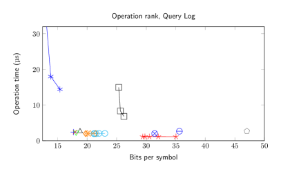
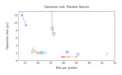
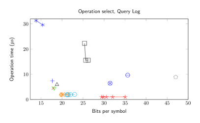
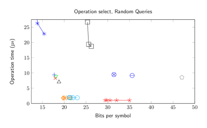
Figure 3: Experimental results for operations $\mathsf{rank}$ (above) and $\mathsf{select}$ (below) on the Wikipedia text. The $x$ axis starts at $H_{0}(s)=12.45$ bits.

Figure 3 shows the experimental results for operations $\mathsf{rank}$ and $\mathsf{select}$, comparing with the most efficient approaches implemented in sdsl. As it can be seen, ASAP yields interesting trade-offs. In particular, for operation $\mathsf{select}$ and random symbols, alternative ASAP GMR-WM (D 23) uses 1.11 times the space of AP, and improves the average time per $\mathsf{select}$ by 79.50% (from 9.37 to 1.92 microseconds per $\mathsf{select}$). For query-log symbols, we obtain similar results. However, this time there is another interesting alternative: ASAP WM-AP (S) uses only 1.01 times the space of AP (i.e., an increase of about 1%), and improves the average $\mathsf{select}$ time by 38.80%. For $\mathsf{rank}$ queries we improve query time between 4.78% to 17.34%. In this case the improvements are smaller compared to $\mathsf{select}$. This is because operation $\mathsf{rank}$ on bit vectors sd_vector<> is not as efficient as $\mathsf{select}$ [47], and AP uses $\mathsf{rank}$ on the bit vectors of the Huffman-shaped WT that implements mapping $t$.

Figure 4 shows experimental results for operation $\mathsf{access}$. As expected, we cannot compete with the original AP scheme. However, we are still faster than RRR-WT, and competitive with GMR [32] (yet using much less space).

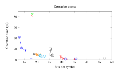
Figure 4: Experimental results for operation access. The $x$ axis starts at $H_{0}(s)=12.45$ bits.

4 Experimental Results on Information-Retrieval Applications

We test in this section our alphabet-partitioning implementation on some relevant applications.

4.1 Application 1: Snippet Extraction

We evaluate next the snippet extraction task, common in text search engines [6, 52]. As we have already said, in this case one needs operation $\mathsf{access}$ to obtain not just a single symbol, but a snippet $s[i..i+L-1]$ of $L$ consecutive symbols in $s$. In our experiments we tested with $L=$ 100 and 200 (see Figure 5).

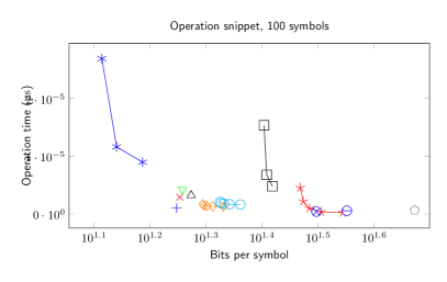
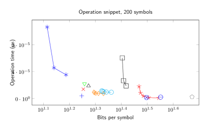
Figure 5: Experimental results for extracting snippets of length $L=100$ (right) and $L=200$ (left). The $x$ axis starts at $H_{0}(s)=12.45$ bits.

As it can be seen, we are able to reduce the time per symbol considerably (approximately by 75%) when compared with operation $\mathsf{access}$, making our approach more competitive for snippet extraction. It is important to note that operation $B_{j}.\mathsf{select}$ in line 7 of Algorithm 1 is implemented using the $\mathsf{select}$ operation provided by the sd_vector<> implementation.

4.2 Application 2: Intersection of Inverted Lists

Another relevant application of $\mathsf{rank}$/$\mathsf{select}$ data structures is that of intersecting inverted lists. A previous work [4] has shown that one can simulate the intersection of inverted lists by representing the document collection (concatenated into a single string) with a $\mathsf{rank}$/$\mathsf{select}$ data structure. So, within the compressed space used by the text collection, one is able to simulate:

• the inverted index of the text collection, supporting intersection of (the simulated) inverted lists in time close to that of Barbay and Kenyon adaptive intersection time [14, 4];

• a positional inverted index, using the approach by Arroyuelo et al. [6]; and

• snippet extraction.

These cover most functionalities of a search engine on document collections, making it an attractive approach because of its efficient space usage.

Figure 6 shows experimental results for intersecting inverted lists. We implemented the variant of intersection algorithm tested by Barbay et al. [13]. As it can be seen, ASAP yields important improvements in this application: using only 2% extra space, ASAP wm-wm (S) is able to reduce the intersection time of AP by 60.67%.

Figure 6: Experimental results for inverted list intersection. Times are in milliseconds. The $x$ axis starts at $H_{0}(s)=12.45$ bits.

5 Alphabet Partitioning for Representing Strings with Runs

Let us consider next the case where the input string $s$ is formed by $r$ runs of equal symbols. Formally, let $s=c_{1}^{l_{1}}c_{2}^{l_{2}}\cdots c_{r}^{l_{r}}$, where $c_{i}\in\Sigma$, for $i=1,\ldots,r$, $l_{1},l_{2},\ldots,l_{r}>0$, $c_{i}\not=c_{i+1}$ for all $1\leq i<r$, and $2\leq\sigma\leq r$.

We study first how to implement run-length compression with the original alphabet partitioning approach [13], to then analyze the scheme resulting from our approach. Notice that the alphabet partition does not need to be carried out according to Equation (3), whose main objective was to distribute the alphabet symbols within the sub-alphabets in such a way $H_{0}(s)$ compression is achieved. As we aim at run-length compression now, we partition in a different —much simpler— way. We divide the alphabet into $p=\lceil\lg{n}\rceil$ subalphabets consisting of $\lceil\sigma/\lceil\lg{n}\rceil\rceil$ alphabet symbols each (the last partition can have less symbols). In this way,

$$m[\alpha]=\frac{\alpha}{\lceil\sigma/\lceil\lg{n}\rceil\rceil},$$

which can be computed on the fly when needed, without storing mapping $m$, saving non-negligible space [13]. Every symbol $\alpha\in\Sigma_{\ell}$ is reenumerated as $\alpha\bmod{(\lceil\sigma/\lceil\lg{n}\rceil\rceil)}$.

Notice that the $r$ runs in the input string are also transferred to mapping $t$ and the sub-alphabet strings $s_{\ell}$. Moreover, the number of runs in mapping $t$ and strings $s_{\ell}$ can be smaller than $r$. For $t$, if symbols $c_{j},c_{j+1},\ldots,c_{j+k}$ (for $1\leq j\leq r$, $k\geq 0$ and $j+k\leq r$) correspond to the same sub-alphabet, then $t$ will have a single run of length $l_{j}+l_{j+1}+\cdots+l_{j+k}$ whereas $s$ has $j+k$ runs corresponding to them. Let us call $r^{(t)}\leq r$ the number of runs in mapping $t$. Similarly, there can be symbols $c_{j}=c_{j+k}=\cdots=c_{j+m}$ (i.e., equal symbols whose runs are not consecutive in $s$) that could form a single run of length $l_{j}+l_{j+k}+\cdots+l_{j+m}$ in the corresponding string $s_{\ell}$. Let us call $r_{\ell}$, $\ell=0,\ldots,p-1$, the number of runs in $s_{\ell}$. Also, let us denote $r^{(s)}=\sum_{\ell=0}^{p-1}{r_{\ell}}\leq r$. Reducing the overall number of runs is one of the advantages of using alphabet partitioning for run-length encoded strings, as we show next.

For mapping $t$, which has alphabet $p=\lceil\lg{n}\rceil$, we use Fuentes-Sepúlveda et al. [29] data structure, requiring $(1+\epsilon)r^{(t)}\lg{\frac{n\lg{n}}{r^{(t)}}}+O\!\left(r^{(t)}\right)$ bits. For the sub-alphabet strings $s_{\ell}$, since all of them have alphabets of size $\sigma_{\ell}=\lceil\sigma/\lceil\lg{n}\rceil\rceil$, we concatenate them into a single string $s^{\prime}$ of length $n$ and $r^{(s)}$ runs . We then also use Fuentes-Sepúlveda et al. data structure for $s^{\prime}$, using $(1+\epsilon)r^{(s)}\lg{\frac{n\sigma}{r^{(s)}\lg{n}}}+O\!\left(r^{(s)}\right)$ additional bits of space.

Next, we consider replacing $t$ with bit vectors $B_{0},\ldots,B_{p}$, as before. In particular, we concatenate them into a single bit vector $B[1{..}n\lg{n}]$, with $n$ 1s and $r^{(t)}$ runs of 1. According to Arroyuelo and Raman [10], bit vector $B$ can be represented using $\lg{n\lg{n}-n+1\choose r^{(t)}}+\lg{n-1\choose r^{(t)}-1}$, which by Stirling approximation is about $r^{(t)}\lg{\frac{n\lg{n}}{r^{(t)}}}+r^{(t)}\lg{\frac{n}{r^{(t)}}}=2r^{(t)}\lg{\frac{n}{r^{(t)}}}+r^{(t)}\lg{\lg{n}}$ bits, Operation $\mathsf{rank}$ is supported in time $O\!\left(\lg{\frac{\lg{(n\sigma/(r^{(s)}\lg{n}))}}{\lg\lg{n}}}\right)$, whereas $\mathsf{select}$ takes time $O\!\left(\lg{\frac{\lg{(n/r^{(s)})}}{\lg\lg{n}}}\right)$. This scheme uses slightly more space (depending on the value of $\epsilon$) than the space used by $t$ of the original alphabet-partitioning approach. However, using bit vector $B$ instead of $t$ allows for a faster implementation in practice (as we will see in our experiments of Section 6).

So, alphabet partitioning on run-length compressed strings has the advantage of potentially reducing the number of runs needed to represent the original string, so the space usage of the data structure depends on $r^{(t)}$ and $r^{(s)}$, rather than on $r$.

6 Application 3: Full-Text Search on Big-Alphabet Highly-Repetitive Collections

Several applications deal with highly-repetitive texts, that is, texts where the amount of repetitiveness is high. Typical examples are:

1. Biological databases, where the DNA of different individuals of the same species share a high percentage of their sequences [38];

2. Source code repositories, where the different (highly-similar) versions of a source code are stored; and

3. The Wikipedia Project, where the different (highly-similar, in general) versions of Wikipedia pages need to be stored.

These are just a few examples of this kind of text databases that are common nowadays. We are particularly interested in big-alphabet highly-repetitive text collections, as big-alphabets are the most suitable for the alphabet-partitioning approach. These text databases usually need to be searched to find patterns of interest, while using compressed space [46]. We are interested in the classical full-text search problem in this section, defined as follows. Let $T[1{..}n]$ be a text string of length $n$ over an alphabet $\Sigma$, and let $P[1{..}m]$ be another string (the search pattern) of length $m$ over the same alphabet $\Sigma$. The problem consists in finding (or counting) all occurrences of $P$ in $T$. We assume the offline version of the problem, where the text is given in advance to queries and several queries will be carried out on the text. Hence, one can afford building a data structure on the text to later speed-up queries. Several solutions to this problem, such as suffix trees [54, 42, 2], suffix arrays [40], and compressed full-text indexes [28, 35, 8]. We show next that our alphabet-partitioning implementation for strings with runs from Section 5 is a competitive building block for implementing compressed-suffix arrays indexes [28, 30].

An effective compression approach that improves space usage while supporting search functionalities is the Burrows-Wheeler transform [18, 28] (BWT, for short). In particular, for highly-repetitive texts the BWT tends to generate long runs of equal symbols [30]. We test next this application, representing the BWT of a text using our ASAP data structure. On it, we implement the backward search algorithm by Ferragina and Manzini [28], which carries out $\Theta(m)$ $\mathsf{rank}$s on the BWT to count the number of occurrences of a pattern $P[1{..}m]$ in the original text.

6.1 Text Collections

We test with the BWT of the following highly-repetitive texts from the Pizza&Chili Corpus [27] :

• Einstein.de: A single sequence containing the concatenation of the different versions of the Wikipedia articles corresponding to Albert Einstein, in German. The original text can be obtained from http://pizzachili.dcc.uchile.cl/repcorpus/real/einstein.de.txt.gz. To obtain a big alphabet, we use the following technique from natural-language text processing: we enumerate all words and punctuation marks in the text, and use a 32-bit integer array to represent it. The result is a sequence of 29,970,916 symbols, with an alphabet of size 7,105. The BWT of this text has 40,349 runs.

• Einstein.en: Similar as before, this time with the Wikipedia articles corresponding to Albert Einstein in English. This text can be obtained from http://pizzachili.dcc.uchile.cl/repcorpus/real/einstein.en.txt.gz. We used the same representation as before, obtaining a sequence of 159,119,879 words and quotation marks, with an alphabet of size 15,862. The BWT of this text has 96,953 runs.

• English: The sequence obtained from the concatenation of English text files selected from etext02 to etext05 collections of the Gutenberg Project. This text can be obtained from http://pizzachili.dcc.uchile.cl/repcorpus/pseudo-real/english.001.2.gz. We use the same representation as before, obtaining a text of 39,894,587 symbols and alphabet of size 89,753. The number of runs in the BWT of this text is 644,502.

• Coreutils: all versions 5.x of the Coreutils package, with a total of 9 versions. We also collected all 1.0.x and 1.1.x versions of the Linux Kernel, with a total of 36 versions http://pizzachili.dcc.uchile.cl/repcorpus/real/coreutils.gz.

Table 3 shows a summary of the main statistics of these texts.

Table 3: Statistics of the highly-repetitive texts used in our tests.

Text	Length	Alphabet size	BWT runs	Avg. run length
Einstein.de	29,970,946	7,105	40,349	742
Einstein.en	159,119,879	15,862	96,953	1,640
English	39,894,587	89,753	644,502	61
Coreutils	93,319,681	148,654	2,540,091	36

We implement the data structure from Section 5, trying the following approaches for its main components. We engineer next the different components.

6.2 Practical Run-Length Compressed Bit Vectors

We survey in this section approaches for compressing bit vectors with runs of 1s, in order to decide the best alternative for $B_{0},\ldots,B_{p-1}$. In particular, we test the following approaches.

$\mathtt{PEF}$

The Partitioned Elias-Fano (PEF) approach [48]. We re-implemented this scheme based on the original one, adding the capabilities for $\mathsf{rank}$ and $\mathsf{select}$ (as the original one only supported the next-greater-or-equal operation). We only test with the Optimized Partition approach (opt), as this is the one that uses the least space. The main idea is that the original bit vector is divided into blocks such that: (1) each block is represented either as a plain bit vector, an SDArray, or it is represented implicitly if it consists only of 1s; and (2) the overall space usage obtained from this partitioning is optimized .

We parameterized the minimum size a block can have as 64, 128, 256, 512, 1024, and 2048. That is, the approach determines the optimal block sizes having into account that no block can be smaller than these values. For the blocks represented with plain bit vectors, we tested with bit_vector<> from the sdsl and Vigna’s broad-word approach [53] (https://github.com/vigna/sux). For the former, we tested with rank_suppor_v and rank_support_v5 in order to provide different space/time trade-offs. However, and since we use these approaches to represent relatively small bit vectors, we modified the original implementation of both rank support data structures such that the precomputed rank information now is stored using an array of $\lg{u}$-bit integers, being $u$ the length of the bit vector. The original implementation used an array of 64-bit integers. We divided the bit vector into blocks of 512 bits. Hence, we store a second-level array of 9-bit integers, as the precomputed values in this level are local to a block. For blocks represented with SDArray we use sd_vector<> from the sdsl. The source code of our implementation can be accessed at https://github.com/Yhatoh/PEF.

$\mathtt{S18}$

The $\mathsf{rank}$/$\mathsf{select}$ data structure based on S18 compression [9, 12]. We used block sizes 8, 16, 32, 64, 128, and 256. The source code of this approach is at https://github.com/HectorxH/Modificacion-S18.

$\mathtt{hyb\_vector}$

The hyb_vector<> data structure from the sdsl, using block size 16.

$\mathtt{Zombit}$

The data structure by Gómez-Brandón [34]. This data structure only implements operation $\mathsf{rank}$, and the source code can be accessed at https://github.com/adriangbrandon/zombit/blob/main/include/zombit_vector.hpp.

$\mathtt{OZ}$

The approach by Delpratt et al. [25], which stores the lengths of the 0 and 1 runs using two separate arrays, Z and O [46, see Section 4.4.3]. We use an implementation provided by Gómez-Brandón [34], where these arrays are represented using sd_vector<> from the sdsl.

$\mathtt{RLE\_VECTOR}$

The approach tested by Boffa et al. [16], which implements scheme OZ yet using VNibble compression [6].

Experimental Survey

In order to choose the most efficient trade-offs, we test experimentally using 1,000,000 random $\mathsf{rank}$ and $\mathsf{select}$ queries on the $p$ bit vectors of the ASAP data structure corresponding to each text we tested. Figure 7 shows the space-time trade-off for operations $\mathsf{rank}$ and $\mathsf{select}$. Regarding space usage, we report the average over the $p$ bit vectors.

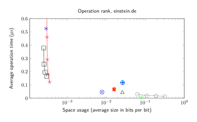
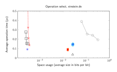
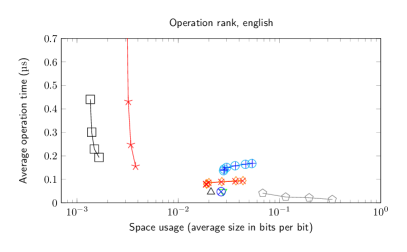
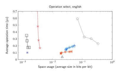
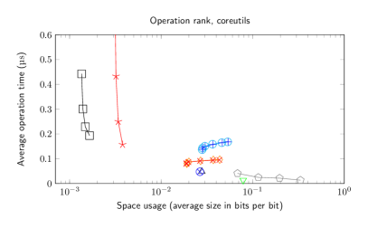
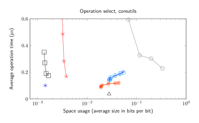
Figure 7: Experimental space/time trade-offs for different compressed bit vector approaches on bit sequences with runs. Results for operation $\mathsf{rank}$ are shown in the left column, whereas $\mathsf{select}$ is shown in the right column.

As it can be seen, RLE_VECTOR and S18 offer the best trade-offs for $\mathsf{rank}$ and $\mathsf{select}$, so we will use them in the following experiments. OZ is also competitive yet just for $\mathsf{select}$. As backward search only needs $\mathsf{rank}$, we disregard it in what follows.

6.3 Practical Run-Length Compressed Strings

For the sub-alphabet strings $s_{0},\ldots,s_{p-1}$ we test the following run-length-compression approaches:

• RLMN: the run-length wavelet tree by Mäkinen and Navarro [39], implemented with class wt_rlmn in the sdsl.

• FKKP: the run-length data structure by Fuentes-Sepúlveda et al. [29]. We use the original implementations by the authors, obtained from https://github.com/jfuentess/sdsl-lite.

We tried the possible combinations among these approaches and RLE_VECTOR or S18, obtaining the 10 schemes denoted by the following regular expression:

$$\texttt{ASAP}~{}(\texttt{AP(RLMN)}~{}|~{}\texttt{RLMN(AP)}~{}|~{}\texttt{RLMN(INT)}~{}|~{}\texttt{FKKP(AP)}~{}|~{}\texttt{FKKP(GMR)})~{}~{}(\texttt{RLE}~{}|~{}\texttt{S18})$$

The second term in the regular expression corresponds to the representation for $s_{0},\ldots,s_{p-1}$, where we use:

• AP(RLMN): the alphabet partitioning approach [13] implemented by class wt_ap<> in the sdsl. We used the RLMN approach [39] for $t$ and the sub-alphabet sequences $s_{i}$ (we used wt_rlmn<> from the sdsl).

• RLMN(AP) and RLMN(INT): the approach by Mäkinen and Navarro [39], using the wt_rlmn<> implementation from the sdsl. We use AP as the base data structure (first approach) and a wavelet tree wt_int<> from the sdsl (second approach).

• FKKP(AP) and FKKP(GMR): the approach by Fuentes-Sepúlveda et al. [29], using AP [13] and GMR [32] (wt_gmr<> in the sdsl) as building blocks.

We compared with the baseline approaches AP(RLMN), RLMN(AP), FKKP(AP), and FKKP(GMR), this time to represent the original BWT —yet with the same meaning as explained before to represent the sub-alphabet sequences $s_{i}$.

In our experiments, we searched for 50,000 unique random patterns of length $m=4,8$, and $16$ words. To generate the patterns, we choose a random position within the corresponding text and then extract $m$ words from that position. Figure 8 shows the space/time trade-offs for counting the number of occurrences of a pattern using the backward search algorithm [28].

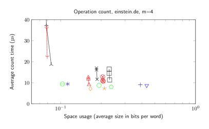
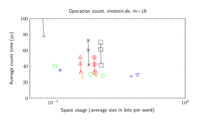
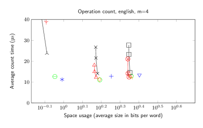
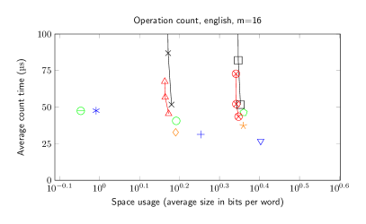
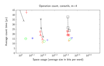
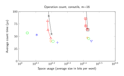
Figure 8: Space/time trade-off for count queries on the Burrows-Wheeler Transform of different big-alphabet texts, using patterns of length 4 and 16.

We show the average search time per pattern searched, and the space usage of each scheme, in bits per text word.

7 Distributed Computation of $\mathsf{rank}$ and $\mathsf{select}$

The partitions generated by the alphabet partitioning approach are amenable for the distributed computation of batches of $\mathsf{rank}$ and $\mathsf{select}$ operations. In this section we explore ways to implement then on a distributed scheme. In a distributed query processing system, there exists a specialized node that is in charge of receiving the query requests (this is called the broker) [20], and then distributes the computation among a set of computation nodes (or simply processors). The latter are in charge of carrying out the actual computation. Next, we study how the original alphabet partitioning scheme (AP) and our proposal (ASAP) can be implemented on a distributed system, allowing the fast computation of batches of $\mathsf{rank}$ and $\mathsf{select}$ queries.

7.1 A Distributed Query-Processing System Based on AP

The sub-alphabet sequences $s_{\ell}$ are distributed among the computation nodes, hence we have $p$ processors in the system. We also have a specialized broker, storing mappings $m$ and $t$. This is a drawback of this approach, as these mappings become a bottleneck for the distributed computation.

7.2 A Distributed Query-Processing System Based on ASAP

In this case, the sub-alphabet sequences $s_{\ell}$ and the bit vectors $B_{\ell}$ are distributed among the computation nodes. Unlike AP, now each computation node acts as a broker: we only need to replicate the mapping $m$ in them. The overall space usage for this is $O(p\sigma\lg{\lg{p}})$ if we use an uncompressed WT for $m$. This is only $O(\sigma\lg\lg{p})=o(n)H_{0}(s)$ bits per processor [13]. In this simple way, we avoid having a specialized broker, but distribute the broker task among the computation nodes. This avoids bottlenecks at the broker, and can make the system more fault tolerant.

Queries arrive at a computation node, which uses mapping $m$ to distribute it to the corresponding computation node. For operation $s.\mathsf{access}(i)$, we carry out a broadcast operation, in order to determine for which processor $\ell$, $B_{\ell}[i]=\mathtt{1}$; this is the one that must answer the query. For extracting snippets, on the other hand, we also broadcast the operation to all processors, which collaborate to construct the desired snippet using the symbols stored at each partition.

7.3 Comparison

The main drawback of the scheme based on AP is that it needs a specialized broker for $m$ and $t$. Thus, the computation on these mappings is not distributed, lowering the performance of the system. The scheme based on ASAP, on the other hand, allows a better distribution: we only need to replicate mapping $m$ in each processor, with a small space penalty in practice. To achieve a similar distribution with AP, we would need to replicate $m$ and $t$ in each processor, increasing the space usage considerably. Thus, given a fixed amount of main memory for the system, the scheme based on ASAP would be likely able to represent a bigger string than AP.

Table 4 shows experimental results on a simulation of these schemes. We only consider computation time, disregarding communication time.

Table 4: Experimental results for the distributed computation of operations on a string. Times are in microseconds per operation, on average (for extracting snippets, it is microseconds per symbol). For $\mathsf{rank}$ and $\mathsf{select}$, the symbols used are from our query log. Scheme ASAP implements the sequences $s_{\ell}$ using wavelet matrices, whereas mapping $m$ is implemented using a Huffman-shaped WT. The partitioning is dense $\ell_{min}=\lg{23}$. The number of partitions generated (i.e., computation nodes in the distributed system) is 46.

Operation		$\mathsf{ASAP}$				$\mathsf{AP}$				AP/ASAP
		Time		Speedup		Time		Speedup
$\mathsf{rank}$		0,373		8.03		1.310		1.91		3.51
$\mathsf{select}$		0.706		8.41		2.970		2.55		4.21
$\mathsf{access}$		1.390		8.11		2.130		1.45		1.53
$\mathsf{snippet}$		0.466		6.96		0.939		1.25		2.02

As it can be seen, ASAP uses the distributed system in a better way. The average time per operation for operations $\mathsf{rank}$ and $\mathsf{select}$ are improved by about 71% and 76%, respectively, when compared with AP. For extracting snippets, the time per symbol extracted is reduced by about 50%. Although the speedup for 46 nodes might seem not too impressive (around 7–8), it is important to note that our experiments are just a proof of concept. For instance, the symbols could be distributed in such a way that the load balance is improved.

8 Conclusions

Our alphabet-partitioning $\mathsf{rank}$/$\mathsf{select}$ data structure offers interesting trade-offs. Using slightly more space than the original alphabet-partitioning data structure from [13], we are able to reduce the time for operation $\mathsf{select}$ by about $80\%$. The performance for $\mathsf{rank}$ can be improved between 4% and 17%. For the inverted-list intersection problem, we showed improvements of about 60% for query processing time, using only 2% extra space when compared to the original alphabet-partitioning data structure. This makes this kind of data structures more attractive for this relevant application in information retrieval tasks.

We also studied how the alphabet-partitioning data structures can be used for the distributed computation of $\mathsf{rank}$, $\mathsf{select}$, $\mathsf{access}$, and $\mathsf{snippet}$ operations. As far as we know, this is the first study about the support of these operation on a distributed-computing environment. In our experiments, we obtained speedups from 6.96 to 8.41, for 46 processors. This compared to 1.25–2.55 for the original alphabet-partitioning data structure. Our results were obtained simulating the distributed computation, hence considering only computation time (and disregarding communication time). The good performance observed in the experiments allows us to think about a real distributed implementation. This is left for future work, as well as a more in-depth study that includes aspects like load balance, among others.

Overall, from our study we can conclude that our approach can be used to implement the ideas from Arroyuelo at al. [6], such that by representing a document collection as a single string using our data structure (hence using compressed space), one can: (i) simulate an inverted index for the document collection; (ii) simulate tf-idf information (using operation $\mathsf{rank}$); (iii) simulate a positional inverted index (using operation $\mathsf{select}$); (iv) to carry out snippet extraction to obtain snippets of interest from the documents. Implementing an information retrieval system based on these ideas is left as future work.

References

- [1] The Lemur Project. https://lemurproject.org/. Accessed May 21, 2023.
- [2] Alberto Apostolico, Maxime Crochemore, Martin Farach-Colton, Zvi Galil, and S. Muthukrishnan. 40 years of suffix trees. Commun. ACM, 59(4):66–73, 2016.
- [3] D. Arroyuelo, V. Gil-Costa, S. González, M. Marin, and M. Oyarzún. Distributed search based on self-indexed compressed text. Information Processing and Management, 48(5):819–827, 2012.
- [4] D. Arroyuelo, S. González, and M. Oyarzún. Compressed self-indices supporting conjunctive queries on document collections. In Proc. SPIRE, LNCS 6393, pages 43–54, 2010.
- [5] Diego Arroyuelo, José Fuentes-Sepúlveda, and Diego Seco. Three success stories about compact data structures. Communications fo the ACM, 63(11):64–65, 2020.
- [6] Diego Arroyuelo, Senén González, Mauricio Marín, Mauricio Oyarzún, Torsten Suel, and Luis Valenzuela. To index or not to index: Time-space trade-offs for positional ranking functions in search engines. Information Systems, 89:101466, 2020.
- [7] Diego Arroyuelo, Aidan Hogan, Gonzalo Navarro, Juan L. Reutter, Javiel Rojas-Ledesma, and Adrián Soto. Worst-case optimal graph joins in almost no space. In Proc. International Conference on Management of Data (SIGMOD), pages 102–114. ACM, 2021.
- [8] Diego Arroyuelo, Gonzalo Navarro, and Kunihiko Sadakane. Stronger lempel-ziv based compressed text indexing. Algorithmica, 62(1-2):54–101, 2012.
- [9] Diego Arroyuelo, Mauricio Oyarzún, Senén González, and Victor Sepulveda. Hybrid compression of inverted lists for reordered document collections. Information Processing & Management, 54(6):1308–1324, 2018.
- [10] Diego Arroyuelo and Rajeev Raman. Adaptive succinctness. Algorithmica, 84(3):694–718, 2022.
- [11] Diego Arroyuelo and Erick Sepúlveda. A practical alphabet-partitioning rank/select data structure. In Proc. 26th International Symposium on String Processing and Information Retrieval (SPIRE), LNCS 11811, pages 452–466. Springer, 2019.
- [12] Diego Arroyuelo and Manuel Weitzman. A hybrid compressed data structure supporting rank and select on bit sequences. In Proc. 39th International Conference of the Chilean Computer Science Society (SCCC), pages 1–8. IEEE, 2020.
- [13] J. Barbay, F. Claude, T. Gagie, G. Navarro, and Y. Nekrich. Efficient fully-compressed sequence representations. Algorithmica, 69(1):232–268, 2014.
- [14] J. Barbay and C. Kenyon. Alternation and redundancy analysis of the intersection problem. ACM Transations on Algorithms, 4(1):4:1–4:18, 2008.
- [15] Djamal Belazzougui and Gonzalo Navarro. Optimal lower and upper bounds for representing sequences. ACM Transactions on Algorithms, 11(4):31:1–31:21, 2015.
- [16] Antonio Boffa, Paolo Ferragina, and Giorgio Vinciguerra. A learned approach to design compressed rank/select data structures. ACM Transactiond on Algorithms, 18(3):24:1–24:28, 2022.
- [17] Alex Bowe. Multiary Wavelet Trees in Practice. Honours thesis, RMIT University, Australia, 2010.
- [18] M. Burrows and D. J. Wheeler. A block sorting lossless data compression algorithm. Technical Report 124, Digital Equipment Corporation, Palo Alto, California, 1994.
- [19] S. Büttcher, C. Clarke, and G. Cormack. Information Retrieval: Implementing and Evaluating Search Engines. MIT Press, 2010.
- [20] B. Barla Cambazoglu and Ricardo Baeza-Yates. Scalability Challenges in Web Search Engines. Morgan & Claypool Publishers, 2015.
- [21] David R. Clark and J. Ian Munro. Efficient suffix trees on secondary storage (extended abstract). In Proc. 7th Annual ACM-SIAM Symposium on Discrete Algorithms (SODA), pages 383–391. ACM/SIAM, 1996.
- [22] Clark, David. Compact PAT trees. PhD thesis, University of Waterloo, 1997.
- [23] C. Clarke, F. Scholer, and I. Soboroff. TREC terabyte track. https://www-nlpir.nist.gov/projects/terabyte/. Accessed May 21, 2023.
- [24] Francisco Claude, Gonzalo Navarro, and Alberto Ordóñez Pereira. The wavelet matrix: An efficient wavelet tree for large alphabets. Information Systems, 47:15–32, 2015.
- [25] O’Neil Delpratt, Naila Rahman, and Rajeev Raman. Engineering the LOUDS succinct tree representation. In Proc. 5th International Workshop Experimental Algorithms (WEA), LNCS 4007, pages 134–145. Springer, 2006.
- [26] P. Ferragina, G. Manzini, V. Mäkinen, and G. Navarro. Compressed representations of sequences and full-text indexes. ACM Trans. Algorithms, 3(2):20, 2007.
- [27] Paolo Ferragina, Rodrigo González, Gonzalo Navarro, and Rossano Venturini. Compressed text indexes: From theory to practice. ACM Journal of Experimental Algorithmics, 13, 2008.
- [28] Paolo Ferragina and Giovanni Manzini. Indexing compressed text. Journal of the ACM, 52(4):552–581, 2005.
- [29] José Fuentes-Sepúlveda, Juha Kärkkäinen, Dmitry Kosolobov, and Simon J. Puglisi. Run compressed rank/select for large alphabets. In Proc. Data Compression Conference (DCC), pages 315–324. IEEE, 2018.
- [30] Travis Gagie, Gonzalo Navarro, and Nicola Prezza. Fully functional suffix trees and optimal text searching in BWT-runs bounded space. Journal of the ACM, 67(1):2:1–2:54, 2020.
- [31] S. Gog and M. Petri. Optimized succinct data structures for massive data. Softw., Pract. Exper., 44(11):1287–1314, 2014.
- [32] A. Golynski, J. I. Munro, and S. Srinivasa Rao. Rank/select operations on large alphabets: a tool for text indexing. In Proc. SODA, pages 368–373, 2006.
- [33] A. Golynski, R. Raman, and S. Srinivasa Rao. On the redundancy of succinct data structures. In Proc. SWAT, pages 148–159, 2008.
- [34] Adrián Gómez-Brandón. Bitvectors with runs and the successor/predecessor problem. In Data Compression Conference (DCC), pages 133–142. IEEE, 2020.
- [35] R. Grossi, A. Gupta, and J. S. Vitter. High-order entropy-compressed text indexes. In Proc. SODA, pages 841–850, 2003.
- [36] R. Grossi, A. Orlandi, and R. Raman. Optimal trade-offs for succinct string indexes. In Proc. ICALP, Part I, pages 678–689, 2010.
- [37] Guy Jacobson. Space-efficient static trees and graphs. In Proc. 30th Annual Symposium on Foundations of Computer Science (FOCS), pages 549–554. IEEE Computer Society, 1989.
- [38] Veli Mäkinen, Djamal Belazzougui, Fabio Cunial, and Alexandru I. Tomescu. Genome-Scale Algorithm Design: Biological Sequence Analysis in the Era of High-Throughput Sequencing. Cambridge University Press, 2015.
- [39] Veli Mäkinen and Gonzalo Navarro. Succinct suffix arrays based on run-length encoding. Nordic Journal of Computing, 12(1):40–66, 2005.
- [40] Udi Manber and Eugene W. Myers. Suffix arrays: A new method for on-line string searches. SIAM Journal on Computing, 22(5):935–948, 1993.
- [41] G. Manzini. An analysis of the Burrows-Wheeler transform. Journal of the ACM, 48(3):407–430, 2001.
- [42] Edward M. McCreight. A space-economical suffix tree construction algorithm. Journal of the ACM, 23(2):262–272, 1976.
- [43] J. Ian Munro. Tables. In Proc. 16th Conference on Foundations of Software Technology and Theoretical Computer Science (FSTTCS), LNCS 1180, pages 37–42. Springer, 1996.
- [44] J. Ian Munro, Rajeev Raman, Venkatesh Raman, and S. Srinivasa Rao. Succinct representations of permutations. In Proc. 30th International Colloquium on Automata, Languages and Programming (ICALP), LNCS 2719, pages 345–356. Springer, 2003.
- [45] G. Navarro. Wavelet trees for all. Journal of Discrete Algorithms, 25:2–20, 2014.
- [46] G. Navarro. Compact Data Structures - A Practical Approach. Cambridge University Press, 2016.
- [47] D. Okanohara and K. Sadakane. Practical entropy-compressed rank/select dictionary. In Proc. ALENEX, pages 60–70, 2007.
- [48] Giuseppe Ottaviano and Rossano Venturini. Partitioned elias-fano indexes. In Proc. 37th International ACM SIGIR Conference on Research and Development in Information Retrieval (SIGIR), pages 273–282. ACM, 2014.
- [49] M. Pǎtraşcu. Succincter. In Proc. 49th Annual IEEE Symposium on Foundations of Computer Science (FOCS), pages 305–313, 2008.
- [50] R. Raman, V. Raman, and S. Rao Satti. Succinct indexable dictionaries with applications to encoding k-ary trees, prefix sums and multisets. ACM Trans. Algorithms, 3(4):43, 2007.
- [51] A. Said. Efficient alphabet partitioning algorithms for low-complexity entropy coding. In Proc. DCC, pages 183–192, 2005.
- [52] A. Turpin, Y. Tsegay, D. Hawking, and H. Williams. Fast generation of result snippets in web search. In Proc. SIGIR, pages 127–134, 2007.
- [53] Sebastiano Vigna. Broadword implementation of rank/select queries. In Proc. 7th International Workshop Experimental Algorithms (WEA), LNCS 5038, pages 154–168. Springer, 2008.
- [54] Peter Weiner. Linear pattern matching algorithms. In Proc. 14th Annual Symposium on Switching and Automata Theory (SWAT), pages 1–11. IEEE Computer Society, 1973.