An Improved Variational Approximate Posterior for the Deep Wishart Process

Abstract

Deep kernel processes are a recently introduced class of deep Bayesian models that have the flexibility of neural networks, but work entirely with Gram matrices. They operate by alternately sampling a Gram matrix from a distribution over positive semi-definite matrices, and applying a deterministic transformation. When the distribution is chosen to be Wishart, the model is called a deep Wishart process (DWP). This particular model is of interest because its prior is equivalent to a deep Gaussian process (DGP) prior, but at the same time it is invariant to rotational symmetries, leading to a simpler posterior distribution. Practical inference in the DWP was made possible in recent work (“A variational approximate posterior for the deep Wishart process" Ober and Aitchison, 2021a) where the authors used a generalisation of the Bartlett decomposition of the Wishart distribution as the variational approximate posterior. However, predictive performance in that paper was less impressive than one might expect, with the DWP only beating a DGP on a few of the UCI datasets used for comparison. In this paper, we show that further generalising their distribution to allow linear combinations of rows and columns in the Bartlett decomposition results in better predictive performance, while incurring negligible additional computation cost.

1 Introduction

Deep kernel processes (DKPs) [Aitchison et al., 2021] are a class of deep Bayesian models which have the flexibility of neural networks (NNs), but work entirely with Gram matrices. NNs have many tuneable parameters which allow them to automatically adapt to problems, and therefore learn good top-layer representations, which turns out to be very important for complex tasks like image classification [Krizhevsky et al., 2012]. On the other hand, most kernels only have a very small number of tuneable hyperparameters, meaning that the kernel matrices they produce are comparatively rigid, and do not have the ability, that NNs have, to learn flexible top-layer representations. DKPs solve this problem by alternately taking the kernel matrix from the previous layer, and sampling from a distribution over positive semi-definite matrices, centred on the previous kernel. Since DKPs never sample features (except for the final outputs), they are distinct from e.g. deep Gaussian processes [Damianou and Lawrence, 2013] (DGPs), which sample features at every layer.

A particular DKP, called the deep Wishart process (DWP), is of particular interest since Aitchison et al. [2021] showed that its prior is equivalent to the DGP prior. However, they were unable to perform inference in the DWP due to the lack of a sufficiently flexible yet tractable distribution over positive semi-definite matrices to use as an approximate posterior. The first solution to this problem was posed by Ober and Aitchison [2021a], who developed a generalisation of the Bartlett decomposition of the Wishart distribution, and used it as the basis of their approximate posterior in a series of experiments that compared DWPs to DGPs. In theory, purely kernel-based methods should have an advantage over feature-based methods, since Gram matrices are invariant to certain symmetries to which feature-based methods are not, leading to simpler posteriors (see Appendix D2 in Aitchison et al. 2021). However, the experiments in Ober and Aitchison [2021a] showed only minor advantages over DGPs on a fraction of the datasets they tested. In this paper, we extend the generalised (singular) Wishart distributions proposed by Ober and Aitchison [2021a] by introducing parameters that rotate, stretch, and mix the rows and columns of the Bartlett decomposition, and show that this added flexibility in the approximate posterior allows DWPs to consistently match or outperform DGPs on UCI datasets, while adding negligible computation cost.

2 Contributions

Concretely, our contributions are:

• We propose the A-generalised (singular) Wishart and AB-generalised (singular) Wishart distributions, two flexible distributions over positive semi-definite matrices, and we provide full derivations for the densities of these distributions in Appendix A.

• We prove both analytically and empirically that the A/AB-generalised (singular) Wishart families are proper supersets of the generalised (singular) Wishart family proposed by Ober and Aitchison [2021a].

• We show experimentally that our proposed approximate posteriors provide significant performance benefits on UCI datasets, while adding negligible computation cost.

3 Related Work

Perhaps the closest prior work is Ober and Aitchison [2021a], which introduces generalised (singular) Wishart approximate posteriors for the deep Wishart process. However, the performance in that paper was less impressive than one might have expected, indicating that there may be room to further improve the family of approximate posteriors over Gram matrices. We provide such an improvement by introducing A and AB-generalised (singular) Wishart approximate posteriors, which exhibit considerably improved performance over the original approximate posterior from Ober and Aitchison [2021a].

The deep kernel process line of work emerged from Aitchison et al. [2021]. While they introduced the deep Wishart process prior, they were not able to perform inference, as they did not have a suitable approximate posterior (that approximate posterior was developed in Ober and Aitchison 2021a). Instead, they were able to do inference in the alternative deep inverse Wishart process, which (unlike the deep Wishart process) does not have any equivalences to DGPs.

The deep kernel process research direction was originally inspired by work showing that infinite-width Bayesian neural networks have GP-distributed outputs [Lee et al., 2017, Matthews et al., 2018, Novak et al., 2018, Garriga-Alonso et al., 2018]. However, this limit is problematic in that the resulting GP kernel is a fixed, deterministic function of the inputs that cannot be learned from data. Thus, this limit eliminates representation or feature learning, which is perhaps the key mechanism behind the excellent practical performance of neural networks [Yang and Hu, 2020, Aitchison, 2020]. Deep kernel processes [Aitchison et al., 2021] were inspired by infinite width NNs but designed specifically to retain flexible, learned kernels.

Another related approach that enables representation learning in infinite-width NNs is the deep kernel machine (DKM) [Yang et al., 2023, Milsom et al., 2023]. DKMs differ from DKPs slightly because they are deterministic and correspond directly to an infinitely wide DGP with an infinitely wide top layer [Yang et al., 2023].

4 Background

In order to understand deep Wishart processes, it is necessary to first define the Wishart distribution. Our implementation of deep Wishart processes further requires a flexibile approximate posterior. This motivates our proposed A/AB-generalised (singular) Wishart distributions, which in turn are obtained by considering the Bartlett decomposition.

4.1 Wishart distribution

The Wishart distribution is a generalisation of the gamma distribution to positive semi-definite matrices. Suppose we take a matrix ${\mathbf{F}\in\mathbb{R}^{P\times\nu}}$ whose columns ${\mathbf{f}_{\lambda}\in\mathbb{R}^{P}\sim\mathcal{N}(\mathbf{0},\mathbf{\Sigma})}$ are multivariate Gaussian distributed vectors with $\lambda\in\{1,\dotsc,\nu\}$ and $\mathbf{\Sigma}\in\mathbb{R}^{P\times P}$, where $P$ is the number of datapoints. Then,

$$\mathbf{W}\coloneqq\mathbf{F}\mathbf{F}^{T}=\sum_{\lambda=1}^{\nu}\mathbf{f}_{\lambda}\mathbf{f}_{\lambda}^{T}$$ (1)

is said to be Wishart distributed, denoted ${\mathbf{W}\in\mathbb{R}^{P\times P}\sim\mathcal{W}(\mathbf{\Sigma},\nu)}$, with positive definite scale matrix $\mathbf{\Sigma}$ and degrees of freedom $\nu$.

4.2 Deep Wishart Process

The deep Wishart process is a specific instantiation of a deep kernel process [Aitchison et al., 2021]. Moreover, DGPs can be reframed as deep Wishart processes. Consider a DGP model, which samples features $\mathbf{F}_{\ell}\in\mathbb{R}^{P\times\nu_{\ell}}$ at each layer sequentially from a Gaussian process,

$$P(\mathbf{F}_{\ell}\mid\mathbf{F}_{\ell-1})=\prod_{\lambda=1}^{\nu_{\ell}}\mathcal{N}(\mathbf{f}^{\ell}_{\lambda};\,\mathbf{0},\mathbf{K}(\mathbf{F}_{\ell-1})).$$ (2)

The columns $\mathbf{f}^{\ell}_{\lambda}$ are IID multivariate Gaussian random variables, where we apply a kernel function ${k(\cdot,\cdot):\mathbb{R}^{\nu_{\ell}}\times\mathbb{R}^{\nu_{\ell}}\to\mathbb{R}}$ pairwise to the previous layer to form the covariance matrix $\mathbf{K}(\mathbf{F}_{\ell-1})\in\mathbb{R}^{P\times P}$.

With deep kernel processes, instead of working with features $\mathbf{F}_{\ell}$, we work with Gram matrices $\mathbf{G}_{\ell}$,

$$\mathbf{G_{\ell}}=\frac{1}{\nu_{\ell}}\mathbf{F}_{\ell}\mathbf{F}_{\ell}^{T}.$$ (3)

With $\mathbf{F}_{\ell}$ defined by Eq. (2), $\mathbf{G}_{\ell}$ is sampled using the same generative process that defines the Wishart distribution (Sec. 4.1), so we have,

$$\mathbf{G}_{\ell}\mid\mathbf{F}_{\ell-1}\sim\mathcal{W}\left(\frac{1}{\nu_{\ell}}\mathbf{K}(\mathbf{F}_{\ell-1}),\nu_{\ell}\right).$$ (4)

The final ingredient for defining a deep Wishart process is the fact that we can often compute the kernel matrix $\mathbf{K}$ from $\mathbf{G}_{\ell-1}$, without having to know $\mathbf{F}_{\ell-1}$. This is true for many common kernels, including isotropic kernels, which only depend on the average squared euclidean distance $R^{\ell-1}_{ij}$ between datapoints,

$$R_{ij}^{\ell} =\frac{1}{\nu_{\ell}}\sum_{\lambda=1}^{\nu_{\ell}}(F^{\ell}_{i\lambda}-F^{\ell}_{j\lambda})^{2}$$ (5a)

$$=\frac{1}{\nu_{\ell}}\sum_{\lambda=1}^{\nu_{\ell}}{(F^{\ell}_{i\lambda}})^{2}-2F^{\ell}_{i\lambda}F^{\ell}_{j\lambda}+\left(F^{\ell}_{j\lambda}\right)^{2}$$ (5b)

$$=G^{\ell}_{ii}-2G^{\ell}_{ij}+G^{\ell}_{jj}.$$ (5c)

(see Aitchison et al., 2021 for further details). Hence we can use $\mathbf{K}\left(\mathbf{G}_{\ell-1}\right)$, eliminating features to work entirely with gram matrices, defining our deep Wishart process like so,

$$\operatorname{P}\left(\mathbf{G}_{\ell}\mid\mathbf{G}_{\ell-1}\right) =\mathcal{W}\left(\mathbf{G}_{\ell};\,\frac{1}{\nu_{\ell}}\mathbf{K}(\mathbf{G}_{\ell-1}),\nu_{\ell}\right),$$ (6a)

$$\operatorname{P}\left(\mathbf{F}_{L+1}\mid\mathbf{\mathbf{G}_{L}}\right) =\prod_{\lambda}^{\nu_{L+1}}\mathcal{N}\left(\mathbf{f}^{L+1}_{\lambda};\,\mathbf{0},\mathbf{K}(\mathbf{G}_{L})\right),$$ (6b)

where $L$ is the number of hidden layers, $\mathbf{G}_{0}=\frac{1}{\nu_{0}}\mathbf{X}\mathbf{X}^{T}$ for input data $\mathbf{X}\in\mathbb{R}^{P\times\nu_{0}}$, and at the output layer (Eq. 6b) we sample features that can be provided to a likelihood function $\operatorname{P}\left(\mathbf{Y}\mid\mathbf{F}_{L+1}\right)$, e.g. a Gaussian likelihood for regression, or a categorical likelihood for classification.

4.3 Variational Inference in DWPs

As is the case with almost all Bayesian models of reasonable complexity, the true posterior $\operatorname{P}\left(\mathbf{G}_{1},\cdots,\mathbf{G}_{L}\mid\mathbf{X},\mathbf{Y}\right)$ is intractable. We therefore use variational inference (VI), which replaces the true posterior with an approximate posterior $\operatorname{Q}\left(\mathbf{G}_{1},\cdots,\mathbf{G}_{L}\right)$. This distribution is taken from a variational family of distributions with parameters $\phi$, which are optimised to maximise a lower bound on the marginal log-likelihood of the data.

We consider approximate posteriors that factorise layerwise,

$$\operatorname{Q}\left(\mathbf{G}_{1},\cdots,\mathbf{G}_{L}\right)=\prod_{\ell=1}^{L}\operatorname{Q}\left(\mathbf{G}_{\ell}\mid\mathbf{G}_{\ell-1}\right),$$ (7)

where each term $\operatorname{Q}\left(\mathbf{G}_{\ell}\mid\mathbf{G}_{\ell-1}\right)$ is a distribution over positive definite matrices. Note that although the prior of each layer is Wishart distributed, the posterior is not Wishart distributed in general. The seemingly obvious choice for this variational family is the Wishart family itself, but as Aitchison et al. [2021] argued, this is not flexible enough. For $\mathbf{G}\sim\mathcal{W}(\mathbf{\Sigma},\nu)$ (particularly in the case where $\nu$ is fixed), the mean and variance cannot be independently specified since we have

$$\mathbb{E}[\mathbf{G}] =\nu\mathbf{\Sigma},$$ (8a)

$$\mathbb{V}[G_{ij}] =\nu(\Sigma_{ij}^{2}+\Sigma_{ii}\Sigma{jj}).$$ (8b)

The ability to independently specify the variance is critical for an approximate posterior to be able to capture potentially narrow true posteriors, so we need an alternative. Aitchison et al. [2021] also suggested that a non-central Wishart distribution would be flexible enough to use as an approximate posterior, but its density is too expensive to evaluate as part of the training loop. Hence Aitchison et al. [2021] ultimately did not perform inference in the DWP, instead opting to change the model. In a subsequent work, Ober and Aitchison [2021a] introduced the generalised (singular) Wishart distribution, which finally allowed practical inference in DWPs, and which our work builds upon. In order to define that distribution, we first need to recap the Bartlett decomposition.

4.4 The Bartlett decomposition

The Bartlett decomposition [Bartlett, 1933] is a factorisation for Wishart random variables. Specifically, if ${\mathbf{W}\sim\mathcal{W}(\mathbf{I},\nu)}$ is a standard Wishart random variable (that is, it has identity scale matrix, $\mathbf{\Sigma}=\mathbf{I}$), then we have,

$$\mathbf{W}=\mathbf{T}\mathbf{T}^{T},$$ (9)

where $\mathbf{T}$ is lower triangular, with the square of its diagonals Gamma-distributed, and its off-diagonals Gaussian-distributed,

$$\mathbf{T} =\begin{pmatrix}T_{11}&\dotsm&0\\ \vdots&\ddots&\vdots\\ T_{P1}&\dotsm&T_{PP}\\ \end{pmatrix},$$ (10a)

$$\operatorname{P}\left(T_{ii}^{2}\right) =\operatorname{Gamma}\left(T_{ii}^{2};\,\tfrac{\nu-i+1}{2},\tfrac{1}{2}\right),$$ (10b)

$$\operatorname{P}\left(T_{i>j}\right) =\mathcal{N}\left(T_{i>j};\,0,1\right),$$ (10c)

In particular each element of $\mathbf{T}$ is independent. For Wishart distributions with non-identity scale matrices, we can compute the Cholesky decomposition $\mathbf{\Sigma}=\mathbf{L}\mathbf{L}^{T}$, so that $\mathbf{W}=\mathbf{L}\mathbf{T}\mathbf{T}^{T}\mathbf{L}^{T}$ (this follows from the canonical definition of the Wishart using Gaussian vectors).

4.5 Generalised (singular) Wishart Distribution

As shown by Ober and Aitchison [2021a], a generalisation of the Wishart distribution can be obtained by allowing the Bartlett decomposition to be more flexible (and by allowing singular matrices [Srivastava, 2003], since the Wishart ordinarily only supports positive definite matrices). Namely, we can introduce parameters $\alpha_{j},\beta_{j},\mu_{ij},\sigma_{ij}$ such that the decomposition $\mathbf{T}$ has distribution,

$$\mathbf{T} =\begin{pmatrix}T_{11}&\dotsm&0\\ \vdots&\ddots&\vdots\\ T_{\nu 1}&\dotsm&T_{\nu\nu}\\ \vdots&\ddots&\vdots\\ T_{P1}&\dotsm&T_{P\nu}\end{pmatrix},$$ (11a)

$$\operatorname{Q}\left(T_{ii}^{2}\right) =\operatorname{Gamma}\left(T_{ii}^{2};\,\alpha_{i},\beta_{j}\right),\,i\in\{1,\ldots,\nu\},$$ (11b)

$$\operatorname{Q}\left(T_{i>j}\right) =\mathcal{N}\left(T_{i>j};\,\mu_{ij},\sigma_{ij}^{2}\right)$$ (11c)

where, in the singular case of $\nu<P$, $\mathbf{T}$ is now a (tall) rectangular matrix, with the upper square block being lower triangular. This more flexible distribution defines a standard generalised (singular) Wishart random variable, denoted $\mathbf{T}\mathbf{T}^{T}\sim\mathcal{GW}\left(\mathbf{I},\nu,\boldsymbol{\mathbf{\alpha}},\boldsymbol{\mathbf{\beta}},\boldsymbol{\mathbf{\mu}},\boldsymbol{\mathbf{\sigma}}\right)$. For the more general case of $\mathbf{\Sigma}\neq\mathbf{I}$, we compute the cholesky decomposition $\mathbf{\Sigma}=\mathbf{L}\mathbf{L}^{T}$ and obtain $\mathbf{W}\sim\mathcal{GW}\left(\boldsymbol{\mathbf{\Sigma}},\nu,\boldsymbol{\mathbf{\alpha}},\boldsymbol{\mathbf{\beta}},\boldsymbol{\mathbf{\mu}},\boldsymbol{\mathbf{\sigma}}\right)$ as $\mathbf{W}=\mathbf{L}\mathbf{T}\mathbf{T}^{T}\mathbf{L}^{T}$.

For the general case $\mathbf{W}=\mathbf{LT}\mathbf{T}^{T}\mathbf{L}^{T}$,  Ober and Aitchison [2021a] showed that the density of $\mathbf{W}$ is

$$\operatorname{Q}\left(\mathbf{W}\right)=\left(\prod_{j=1}^{P}\frac{1}{L_{jj}^{\min(j,\nu)}}\right)\\ \prod_{j=1}^{{\tilde{\nu}}}\frac{\operatorname{Gamma}\left(T_{jj}^{2};\,\alpha_{j},\beta_{j}\right)}{T_{jj}^{P-j}L_{jj}^{P-j+1}}\prod_{i=j+1}^{P}\mathcal{N}\left(T_{ij};\,\mu_{ij},\sigma_{ij}^{2}\right).$$ (12)

5 Methods

5.1 $\mathrm{A}\text{-}\mathcal{GW}$ and $\mathrm{AB}\text{-}\mathcal{GW}$ distributions

Whilst the generalised (singular) Wishart distribution represented a big step for approximate inference in DWPs, the experimental results in Ober and Aitchison [2021a] indicated much room for improvement. Despite the theoretical advantages that DWPs have over DGPs due to their invariance to certain posterior symmetries, the DGP still outperformed the DWP in a few cases. By contrast, the A-generalised / AB-generalised (singular) Wishart distributions we introduce in this paper allow the DWP to match or outperform the DGP on all datasets we tested.

One issue with the generalised (singular) Wishart distribution is that it is unclear how flexible it is with respect to linear transformations. Suppose $\mathbf{W}\sim\mathcal{GW}\left(\boldsymbol{\mathbf{\Sigma}},\nu,\boldsymbol{\mathbf{\alpha}},\boldsymbol{\mathbf{\beta}},\boldsymbol{\mathbf{\mu}},\boldsymbol{\mathbf{\sigma}}\right)$ and consider the mapping $\mathbf{W}\mapsto\mathbf{W}^{\prime}=\mathbf{R}\mathbf{W}\mathbf{R}^{T}$, where ${\mathbf{R}\in\mathbb{R}^{P\times P}}$ is some invertible matrix. With $\mathbf{W}$ constructed as in Section 4.5, i.e. $\mathbf{W}=\mathbf{LT}\mathbf{T}^{T}\mathbf{L}^{T}$, where $\mathbf{T}\mathbf{T}^{T}\sim\mathcal{GW}\left(\mathbf{I},\nu,\boldsymbol{\mathbf{\alpha}},\boldsymbol{\mathbf{\beta}},\boldsymbol{\mathbf{\mu}},\boldsymbol{\mathbf{\sigma}}\right)$ and $\mathbf{\Sigma}=\mathbf{L}\mathbf{L}^{T}$, we have $\mathbf{W}^{\prime}=\mathbf{R}\mathbf{L}\mathbf{T}\mathbf{T}^{T}\mathbf{L}\mathbf{R}^{T}$. However, since ${\mathbf{R}\mathbf{L}}$ is not in general lower triangular, there is no obvious form that suggests $\mathbf{W}^{\prime}$ is in general distributed as a generalised (singular) Wishart. To remedy this, we introduce more flexibility into the generalised (singular) Wishart distribution. In particular, instead of parameterising the distribution in terms of $\boldsymbol{\mathbf{\Sigma}}$, and multiplying $\mathbf{T}$ by the Cholesky of $\boldsymbol{\mathbf{\Sigma}}$, we both parameterise the distribution and multiply $\mathbf{T}$ with an arbitrary invertible matrix of parameters ${\mathbf{A}\in\mathbb{R}^{P\times P}}$. We write $\mathbf{W}=\mathbf{A}\mathbf{T}(\mathbf{A}\mathbf{T})^{T}\sim\mathrm{A}\text{-}\mathcal{GW}\left(\mathbf{A},\nu,\boldsymbol{\mathbf{\alpha}},\boldsymbol{\mathbf{\beta}},\boldsymbol{\mathbf{\mu}},\boldsymbol{\mathbf{\sigma}}\right)$ and say that $\mathbf{W}$ is A-generalised (singular) Wishart distributed. If $\mathbf{W}$ is A-generalised (singular) Wishart distributed, it is clear that for any transformation $\boldsymbol{\mathbf{R}}$, the associated Gram matrix $\boldsymbol{\mathbf{\mathbf{W}}}^{\prime}$ remains in the same family of distributions; in particular, $\mathbf{W}^{\prime}=\boldsymbol{\mathbf{R}}\mathbf{W}\boldsymbol{\mathbf{R}}^{T}\sim\mathrm{A}\text{-}\mathcal{GW}\left(\boldsymbol{\mathbf{R}}\mathbf{A},\nu,\boldsymbol{\mathbf{\alpha}},\boldsymbol{\mathbf{\beta}},\boldsymbol{\mathbf{\mu}},\boldsymbol{\mathbf{\sigma}}\right)$.

We can understand $\mathbf{A}$ in $\mathbf{W}=\mathbf{A}\mathbf{T}(\mathbf{A}\mathbf{T})^{T}$ as mixing the rows of $\mathbf{T}$ by linear combinations. This mixing means that the elements of $\mathbf{A}\mathbf{T}$ have a more complex dependency structure than the elements of $\mathbf{T}$. It also raises the question of whether we could introduce a more complex dependency structure still. We propose that this can be done by additionally mixing the columns of $\mathbf{T}$ with a matrix $\mathbf{B}$, via $\mathbf{T}\mathbf{B}$, suggesting an additional generalisation of the generalised (singular) Wishart distribution. We write ${\mathbf{W}=\mathbf{A}\mathbf{T}\mathbf{B}(\mathbf{A}\mathbf{T}\mathbf{B})^{T}\sim\mathrm{AB}\text{-}\mathcal{GW}\left(\mathbf{A},\mathbf{B},\nu,\boldsymbol{\mathbf{\alpha}},\boldsymbol{\mathbf{\beta}},\boldsymbol{\mathbf{\mu}},\boldsymbol{\mathbf{\sigma}}\right)}$, where ${\mathbf{B}\in\mathbb{R}^{\nu\times\nu}}$ is lower triangular and invertible, and say that $\mathbf{W}$ is AB-generalised (singular) Wishart distributed.

To use the $\mathrm{A}\text{-}\mathcal{GW}$ and $\mathrm{AB}\text{-}\mathcal{GW}$ distributions for VI, it is necessary to obtain expressions for their densities. Since this is non-trivial, the derivations are provided in the Appendix A.7, and we simply quote the results here. The density for the $\mathrm{A}\text{-}\mathcal{GW}$ distribution is,

$$\mathrm{A}\text{-}\mathcal{GW}\left(\mathbf{W};\,\mathbf{A},\nu,\,\boldsymbol{\mathbf{\alpha}},\,\boldsymbol{\mathbf{\beta}},\,\boldsymbol{\mathbf{\mu}},\,\boldsymbol{\mathbf{\sigma}}\right)\\ =\frac{\left\lvert\mathbf{W}_{:{\tilde{\nu}},:{\tilde{\nu}}}\right\rvert^{(\nu-N-1)/2}}{\left\lvert\mathbf{A}\right\rvert^{\nu}\left\lvert(\mathbf{C}_{A})_{:{\tilde{\nu}},:{\tilde{\nu}}}\right\rvert^{(\nu-N-1)/2}}\prod_{j=1}^{\tilde{\nu}}\frac{\operatorname{Gamma}\left(T_{jj}^{2};\,\alpha_{j},\beta_{j}\right)}{T_{jj}^{N-j}}\\ \prod_{i=j+1}^{N}\mathcal{N}\left(T_{ij};\mu_{ij},\sigma_{ij}^{2}\right),$$ (13)

where $\tilde{\nu}=\min\left\{\nu,N\right\}$, $\mathbf{C}_{A}=\mathbf{T}\mathbf{T}^{T}$, and the notation $\boldsymbol{\mathbf{X}}_{:a,:b}$ means the submatrix of $\boldsymbol{\mathbf{X}}$ obtained by taking the first $a$ rows and $b$ columns. The density for the $\mathrm{AB}\text{-}\mathcal{GW}$ distribution is,

$$\mathrm{AB}\text{-}\mathcal{GW}\left(\mathbf{W};\,\mathbf{A},\mathbf{B},\nu,\,\boldsymbol{\mathbf{\alpha}},\,\boldsymbol{\mathbf{\beta}},\,\boldsymbol{\mathbf{\mu}},\,\boldsymbol{\mathbf{\sigma}}\right)\\ =\frac{\left\lvert\mathbf{W}_{:{\tilde{\nu}},:{\tilde{\nu}}}\right\rvert^{(\nu-N-1)/2}}{\left\lvert\mathbf{A}\right\rvert^{\nu}\left\lvert(\mathbf{C}_{AB})_{:{\tilde{\nu}},:{\tilde{\nu}}}\right\rvert^{(\nu-N-1)/2}}\prod_{j=1}^{\tilde{\nu}}\frac{\operatorname{Gamma}\left(T_{jj}^{2};\,\alpha_{j},\beta_{j}\right)}{T_{jj}^{N-j}B_{jj}^{2(N-j+1)}}\\ \prod_{i=j+1}^{N}\mathcal{N}\left(T_{ij};\mu_{ij},\sigma_{ij}^{2}\right),$$ (14)

where $\mathbf{C}_{AB}=(\mathbf{T}\mathbf{B})(\mathbf{T}\mathbf{B})^{T}$ is defined for notational convenience. Notice that the densities are defined in terms of both $\mathbf{W}$ and $\mathbf{T}$. Since $\mathbf{W}=(\mathbf{A}\mathbf{T}\mathbf{B})(\mathbf{A}\mathbf{T}\mathbf{B})^{T}$, we can see that $\mathbf{T}$ can be recovered by first computing $(\mathbf{T}\mathbf{B})(\mathbf{T}\mathbf{B})^{T}=\mathbf{A}^{-1}\mathbf{W}\mathbf{A}^{-T}$, from which we can compute $\mathbf{T}\mathbf{B}$ as the cholesky decomposition. Thus $\mathbf{T}$ is recovered by simply right-multiplying $\mathbf{T}\mathbf{B}$ by $\mathbf{B}^{-1}$.

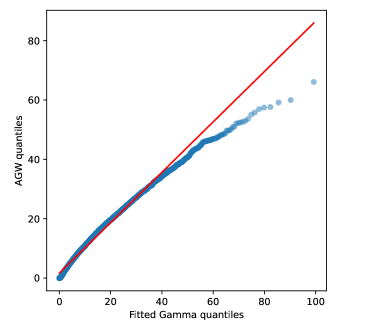
Figure 1: A probability plot comparing the probability density of the top-left element of an $\mathrm{A}\text{-}\mathcal{GW}$ distributed matrix to the density of the top-left element of a $\mathcal{GW}$ distributed matrix. If the two were identically distributed, all the points would lie on the diagonal line. We sampled the top-left element of the $\mathrm{A}\text{-}\mathcal{GW}$ distributed matrix 10,000 times using Eq. (18), Eq. (19) and Eq. (21). We compared this distribution against the closest fitting Gamma distribution, as the top-left element of a $\mathcal{GW}$ distributed matrix is Gamma-distributed (Sec. 5.3). We used $\mu=3,\sigma^{2}=1$ in Eq. (18). In this probability plot, the “Fitted Gamma quantiles” are the exact quantiles of the closest fitting Gamma distribution, while the “AGW quantiles” are the sample quantiles from the top-left element of the $\mathrm{A}\text{-}\mathcal{GW}$ distribution (i.e. the samples ordered by size). The plot shows a clear mismatch between the two distributions, confirming the theoretical result that a Gamma distribution does not capture general non-central chi-squared distributions.

5.2 $\mathrm{A}\text{-}\mathcal{GW}$ and $\mathrm{AB}\text{-}\mathcal{GW}$ approximate posteriors

As discussed in Section 5.1, the A and AB-generalised (singular) Wishart distributions give us more flexible distributions over Gram matrices, which ought to be useful for VI. The approximate posterior used by Ober and Aitchison [2021a] was,

$$\operatorname{Q}_{{\mathcal{GW}}}\left(\mathbf{G}_{\ell}\mid\mathbf{G}_{\ell-1}\right)\\ =\mathcal{GW}\big{(}\mathbf{G}_{\ell};\,(1-q_{\ell})\tfrac{1}{\nu_{\ell}}\mathbf{K}\left(\mathbf{G}_{\ell-1}\right)+q_{\ell}\mathbf{V}_{\ell}{\mathbf{V}}_{\ell}^{T},\\ \nu_{\ell},\,\boldsymbol{\mathbf{\alpha}}_{\ell},\,\boldsymbol{\mathbf{\beta}}_{\ell},\,\boldsymbol{\mathbf{\mu}}_{\ell},\,\boldsymbol{\mathbf{\sigma}}_{\ell}\big{)},$$ (15)

where $\{\mathbf{V}_{\ell},\boldsymbol{\mathbf{\alpha}}_{\ell},\boldsymbol{\mathbf{\beta}}_{\ell},\boldsymbol{\mathbf{\mu}}_{\ell},\boldsymbol{\mathbf{\sigma}}_{\ell},q_{\ell}\}_{\ell=1}^{L}$ are the learned variational parameters. Notice that $\mathbf{V}_{\ell}$ provides flexibility, since $q_{\ell}$ allows us to control the relative influence of the kernel from the previous layer, $\mathbf{K}(\mathbf{G}_{\ell-1})$, and an arbitrary, learnable positive (semi-) definite matrix, $\boldsymbol{\mathbf{V}}_{\ell}\boldsymbol{\mathbf{V}}_{\ell}^{T}$.

To use the A and AB generalised (singular) Wishart distributions as approximate posteriors, we obtain $\mathbf{A}_{\ell}$ by combining an arbitrary invertible matrix of parameters, $\mathbf{A}^{\prime}_{\ell}$, with the Cholesky of $(1-q_{\ell})\tfrac{1}{\nu_{\ell}}\mathbf{K}\left(\mathbf{G}_{\ell-1}\right)+q_{\ell}\mathbf{V}_{\ell}{\mathbf{V}}_{\ell}^{T}$ to give across-layer dependencies similar to those in the previous $\mathcal{GW}$ approximate posterior (Eq. 15),

$$\mathbf{A}_{\ell}=\text{chol}\left((1-q_{\ell})\tfrac{1}{\nu_{\ell}}\mathbf{K}\left(\mathbf{G}_{\ell-1}\right)+q_{\ell}\mathbf{V}_{\ell}{\mathbf{V}}_{\ell}^{T}\right)\mathbf{A}_{\ell}^{\prime}$$ (16)

where $\text{chol}(\cdot)$ returns the lower triangular Cholesky factor. The $\mathrm{A}\text{-}\mathcal{GW}$ and $\mathrm{AB}\text{-}\mathcal{GW}$ approximate posteriors are then written in terms of this $\mathbf{A}_{\ell}$:

$$\operatorname{Q}_{{\mathrm{A}\text{-}\mathcal{GW}}}\left(\mathbf{G}_{\ell}\mid\mathbf{G}_{\ell-1}\right)$$ (17a)

$$\quad\quad\quad=\mathrm{A}\text{-}\mathcal{GW}\big{(}\mathbf{G}_{\ell};\,\mathbf{A}_{\ell},\,\nu_{\ell},\,\boldsymbol{\mathbf{\alpha}}_{\ell},\,\boldsymbol{\mathbf{\beta}}_{\ell},\,\boldsymbol{\mathbf{\mu}}_{\ell},\,\boldsymbol{\mathbf{\sigma}}_{\ell}\big{)},$$

$$\operatorname{Q}_{{\mathrm{AB}\text{-}\mathcal{GW}}}\left(\mathbf{G}_{\ell}\mid\mathbf{G}_{\ell-1}\right)$$ (17b)

$$\quad\quad\quad=\mathrm{AB}\text{-}\mathcal{GW}\big{(}\mathbf{G}_{\ell};\,\mathbf{A}_{\ell},\,\mathbf{B}_{\ell},\,\nu_{\ell},\,\boldsymbol{\mathbf{\alpha}}_{\ell},\,\boldsymbol{\mathbf{\beta}}_{\ell},\,\boldsymbol{\mathbf{\mu}}_{\ell},\,\boldsymbol{\mathbf{\sigma}}_{\ell}\big{)}.$$

Here, the variational parameters are $\{\mathbf{A}^{\prime}_{\ell},\mathbf{V}_{\ell},\boldsymbol{\mathbf{\alpha}}_{\ell},\boldsymbol{\mathbf{\beta}}_{\ell},\boldsymbol{\mathbf{\mu}}_{\ell},\boldsymbol{\mathbf{\sigma}}_{\ell},q_{\ell}\}_{\ell=1}^{L}$ for the $\mathrm{A}\text{-}\mathcal{GW}$ approximate posterior, and $\{\mathbf{A}^{\prime}_{\ell},\mathbf{B}_{\ell},\boldsymbol{\mathbf{V}}_{\ell},\boldsymbol{\mathbf{\alpha}}_{\ell},\boldsymbol{\mathbf{\beta}}_{\ell},\boldsymbol{\mathbf{\mu}}_{\ell},\boldsymbol{\mathbf{\sigma}}_{\ell},q_{\ell}\}_{\ell=1}^{L}$ for the $\mathrm{AB}\text{-}\mathcal{GW}$ approximate posterior.

Table 1: ELBOs, test log-likelihoods, and test root mean square error for UCI datasets from [Gal and Ghahramani, 2016] for a five-layer network. All metrics are quoted as the mean, plus or minus one standard error, over the splits. Better results are highlighted; see Appendix B for other depths and additional information.

				DWP
	Dataset	DGP	$\operatorname{Q}_{\mathcal{GW}}$	$\operatorname{Q}_{\mathrm{A}\text{-}\mathcal{GW}}$	$\operatorname{Q}_{\mathrm{AB}\text{-}\mathcal{GW}}$
	Boston	-0.45 $\pm$ 0.00	-0.37 $\pm$ 0.01	-0.36 $\pm$ 0.00	-0.36 $\pm$ 0.00
	Concrete	-0.50 $\pm$ 0.00	-0.49 $\pm$ 0.00	-0.45 $\pm$ 0.00	-0.45 $\pm$ 0.00
	Energy	1.38 $\pm$ 0.00	1.40 $\pm$ 0.00	1.42 $\pm$ 0.00	1.41 $\pm$ 0.00
	Kin8nm	-0.14 $\pm$ 0.00	-0.14 $\pm$ 0.00	-0.11 $\pm$ 0.00	-0.11 $\pm$ 0.00
ELBO	Naval	3.92 $\pm$ 0.04	3.59 $\pm$ 0.12	3.97 $\pm$ 0.02	3.63 $\pm$ 0.22
	Power	0.03 $\pm$ 0.00	0.02 $\pm$ 0.00	0.03 $\pm$ 0.00	0.03 $\pm$ 0.00
	Protein	-1.00 $\pm$ 0.00	-1.01 $\pm$ 0.00	-1.00 $\pm$ 0.00	-1.00 $\pm$ 0.00
	Wine	-1.19 $\pm$ 0.00	-1.19 $\pm$ 0.00	-1.19 $\pm$ 0.00	-1.19 $\pm$ 0.00
	Yacht	1.46 $\pm$ 0.02	1.59 $\pm$ 0.02	1.79 $\pm$ 0.02	1.79 $\pm$ 0.02
	Boston	-2.43 $\pm$ 0.04	-2.38 $\pm$ 0.04	-2.39 $\pm$ 0.05	-2.38 $\pm$ 0.04
	Concrete	-3.13 $\pm$ 0.02	-3.13 $\pm$ 0.02	-3.07 $\pm$ 0.02	-3.08 $\pm$ 0.02
	Energy	-0.71 $\pm$ 0.03	-0.71 $\pm$ 0.03	-0.70 $\pm$ 0.03	-0.70 $\pm$ 0.03
	Kin8nm	1.38 $\pm$ 0.00	1.40 $\pm$ 0.01	1.41 $\pm$ 0.01	1.41 $\pm$ 0.01
LL	Naval	8.28 $\pm$ 0.04	8.17 $\pm$ 0.07	8.40 $\pm$ 0.02	8.10 $\pm$ 0.19
	Power	-2.78 $\pm$ 0.01	-2.77 $\pm$ 0.01	-2.76 $\pm$ 0.01	-2.76 $\pm$ 0.01
	Protein	-2.73 $\pm$ 0.01	-2.72 $\pm$ 0.01	-2.71 $\pm$ 0.01	-2.70 $\pm$ 0.00
	Wine	-0.96 $\pm$ 0.01	-0.96 $\pm$ 0.01	-0.96 $\pm$ 0.01	-0.96 $\pm$ 0.01
	Yacht	-0.73 $\pm$ 0.07	-0.58 $\pm$ 0.06	-0.22 $\pm$ 0.09	-0.18 $\pm$ 0.07
	Boston	2.81 $\pm$ 0.14	2.82 $\pm$ 0.17	2.77 $\pm$ 0.16	2.81 $\pm$ 0.17
	Concrete	5.49 $\pm$ 0.10	5.53 $\pm$ 0.10	5.26 $\pm$ 0.11	5.24 $\pm$ 0.11
	Energy	0.49 $\pm$ 0.01	0.48 $\pm$ 0.01	0.48 $\pm$ 0.01	0.48 $\pm$ 0.01
	Kin8nm	0.06 $\pm$ 0.01	0.06 $\pm$ 0.01	0.06 $\pm$ 0.00	0.06 $\pm$ 0.00
RMSE	Naval	0.00 $\pm$ 0.00	0.00 $\pm$ 0.00	0.00 $\pm$ 0.00	0.00 $\pm$ 0.00
	Power	3.88 $\pm$ 0.04	3.84 $\pm$ 0.04	3.80 $\pm$ 0.04	3.80 $\pm$ 0.04
	Protein	3.77 $\pm$ 0.02	3.76 $\pm$ 0.02	3.73 $\pm$ 0.02	3.70 $\pm$ 0.01
	Wine	0.63 $\pm$ 0.01	0.63 $\pm$ 0.01	0.63 $\pm$ 0.01	0.63 $\pm$ 0.01
	Yacht	0.57 $\pm$ 0.05	0.50 $\pm$ 0.04	0.37 $\pm$ 0.03	0.38 $\pm$ 0.03

Table 2: Average runtime (seconds) for an epoch of Boston and Protein. Error bars were negligible and are excluded.

{dataset} - {depth}	DGP	$\operatorname{Q}_{\mathcal{GW}}$	$\operatorname{Q}_{\mathrm{A}\text{-}\mathcal{GW}}$	$\operatorname{Q}_{\mathrm{AB}\text{-}\mathcal{GW}}$
Boston - 2	0.463	0.200	0.203	0.202
5	1.292	0.358	0.373	0.370
Protein - 2	0.903	0.843	0.854	0.869
5	2.012	1.806	1.846	1.839

5.3 $\mathrm{A}\text{-}\mathcal{GW}$ is more flexible than $\mathcal{GW}$

To further motivate the utility of the proposed distributions, we now demonstrate that the $\mathrm{A}\text{-}\mathcal{GW}$ family of distributions (Eq. 13) is a proper superset of the $\mathcal{GW}$ family (Eq. 12). The fact that it is a superset can be seen by noting that if we take $\mathbf{A}$ to be lower triangular, and use $\mathbf{\Sigma}=\mathbf{A}\mathbf{A}^{T}$, then the $\mathrm{A}\text{-}\mathcal{GW}$ distribution reduces to the $\mathcal{GW}$ distribution. Note that the $\mathrm{AB}\text{-}\mathcal{GW}$ distribution also reduces to the previous $\mathcal{GW}$ distribution if we take $\mathbf{A}$ to be lower triangular and $\mathbf{B}=\mathbf{I}$. We do not make the claim that the $\mathrm{AB}\text{-}\mathcal{GW}$ distribution is strictly more flexible than the $\mathrm{A}\text{-}\mathcal{GW}$ distribution (though it clearly contains the $\mathrm{A}\text{-}\mathcal{GW}$ by just setting $\mathbf{B}=\mathbf{I}$), and instead leave this to future work.

In order to show that the $\mathrm{A}\text{-}\mathcal{GW}$ family contains a proper superset of $\mathcal{GW}$, we must show it contains distributions which the $\mathcal{GW}$ cannot capture. To this end, consider a toy setting where $P=2$ and $\nu=1$, so, $\boldsymbol{\mathbf{T}}\in\mathbb{R}^{2\times 1}$. We choose this matrix to be,

$$\mathbf{T}\coloneqq\begin{pmatrix}g\\ n\end{pmatrix}\sim\begin{pmatrix}\mathcal{N}\left(0,1\right)\\ \mathcal{N}\left(\mu,\sigma^{2}\right)\end{pmatrix}$$ (18)

so that $g^{2}\sim\chi^{2}\left(1\right)=\operatorname{Gamma}\left(\frac{1}{2},2\right)$. Then we have,

$$\mathbf{W}=\mathbf{A}\mathbf{T}(\mathbf{A}\mathbf{T})^{T}\sim\mathrm{A}\text{-}\mathcal{GW}\left(\mathbf{A},1,\frac{1}{2},2,\mu,\sigma^{2}\right)$$ (19)

where $\mathbf{W}\in\mathbb{R}^{2\times 2}$ and $\mathbf{A}\in\mathbb{R}^{2\times 2}$ is any invertible matrix. We shall show that, for certain choices of $\mathbf{A}$, $\mathbf{W}$ has a distribution that cannot be captured by the $\mathcal{GW}$ distribution. Firstly, we have,

$$\mathbf{T}\mathbf{T}^{T}=\begin{pmatrix}g^{2}&gn\\ gn&n^{2}\end{pmatrix},$$ (20)

and taking $\boldsymbol{\mathbf{A}}$ to have concrete value,

$$\mathbf{A}=\begin{pmatrix}1&1\\ 0&1\end{pmatrix},$$ (21)

we obtain,

$$\left(\mathbf{A}\mathbf{T}\right)\left(\mathbf{A}\mathbf{T}\right)^{T}=\begin{pmatrix}g^{2}+2gn+n^{2}&gn+n^{2}\\ gn+n^{2}&n^{2}\end{pmatrix}.$$ (22)

We need only consider the distribution of the top-left element. We have $g^{2}+2gn+n^{2}=(g+n)^{2}=X^{2}$ where $X\sim\mathcal{N}\left(\mu,\sigma^{2}+1\right)$, since $g$ and $n$ are normally distributed. Hence if we choose $\mu\neq 0$, the top-left element, $X^{2}$, is noncentral chi-squared distributed.

To conclude the proof, we show that the top-left element of a $\mathcal{GW}$-distributed matrix is restricted to a Gamma distribution, which does not contain noncentral chi-squared distributions. In particular, taking $\boldsymbol{\mathbf{\Sigma}}=\mathbf{L}\mathbf{L}^{T}$ to be the cholesky decomposition of $\boldsymbol{\mathbf{\Sigma}}$, any $\mathcal{GW}$-distributed matrix,

$$\mathbf{W}^{\prime}=(\mathbf{L}\mathbf{T}^{\prime})(\mathbf{L}\mathbf{T}^{\prime})^{T}\sim\mathcal{GW}\left(\boldsymbol{\mathbf{\Sigma}},\nu^{\prime},\boldsymbol{\alpha}^{\prime},\boldsymbol{\beta}^{\prime},\boldsymbol{\mu}^{\prime},\boldsymbol{\sigma}^{{}^{\prime}2}\right),$$ (23)

can be written according to the generalised Bartlett decomposition in Eq. 11. To obtain the top-left element of $\mathbf{W}^{\prime}$, we first explicitly write down the first element of $\mathbf{L}\mathbf{T}^{\prime}$,

$$\mathbf{L}\mathbf{T}^{\prime} =\begin{pmatrix}L_{11}&0\\ L_{21}&L_{22}\end{pmatrix}\begin{pmatrix}T^{\prime}_{11}\\ T^{\prime}_{21}\end{pmatrix}=\begin{pmatrix}L_{11}T^{\prime}_{11}\\ \dotsc\end{pmatrix},$$ (24)

where we avoid writing down the second element because it will not be needed. Then, we can explicitly write down the top-left element of the $\mathcal{GW}$ distributed $\mathbf{W}^{\prime}$,

$$\mathbf{W}^{\prime} =\mathbf{L}\mathbf{T}^{\prime}(\mathbf{L}\mathbf{T}^{\prime})^{T}=\begin{pmatrix}L_{11}T^{\prime}_{11}\\ \dotsc\end{pmatrix}\begin{pmatrix}L_{11}T^{\prime}_{11}\\ \dotsc\end{pmatrix}^{T}$$

$$=\begin{pmatrix}L_{11}^{2}(T^{\prime}_{11})^{2}&\dotsc\;\\ \dotsc\;&\dotsc\;\end{pmatrix}.$$ (25)

By Eq. 11b, we have $(T_{11}^{\prime})^{2}\sim\operatorname{Gamma}\left(\alpha_{1}^{\prime},\beta_{1}^{\prime}\right)$, and so the top-left element of $\mathbf{W}$ has distribution

$$W^{\prime}_{11}=L_{11}^{2}(T_{11}^{\prime})^{2}\sim\operatorname{Gamma}\left(\alpha_{1}^{\prime},\frac{\beta_{1}^{\prime}}{L_{11}^{2}}\right).$$ (26)

Since the Gamma distribution is not capable of capturing noncentral chi-square distributions, we conclude that the $\mathrm{A}\text{-}\mathcal{GW}$ family is strictly larger than the $\mathcal{GW}$ family.

Figure 1 shows a probability plot to empirically demonstrate that the $\mathcal{GW}$ distribution is not capable of capturing the $\mathrm{A}\text{-}\mathcal{GW}$ distribution. Specifically, we consider the same $\mathrm{A}\text{-}\mathcal{GW}$ top-left element as in our counter-example above, using $\mu=3,\sigma^{2}=1$ in Eq. 18, and take samples from it. We then fit a Gamma distribution to these samples, and show that there is a clear mismatch.

Algorithm 1 Computing predictions/ELBO for a DWP with $\mathrm{AB}\text{-}\mathcal{GW}$ variational posterior.

  Hyperparameters: $\{\sl{\nu_{\ell}}\}_{\ell=1}^{L}$

  Learned $\operatorname{Q}$ parameters:

   $\{\mathbf{A}_{\ell}^{\prime},\mathbf{B}_{\ell},\boldsymbol{\mathbf{V}}_{\ell},\boldsymbol{\mathbf{\alpha}}_{\ell},\boldsymbol{\mathbf{\beta}}_{\ell},\boldsymbol{\mathbf{\mu}}_{\ell},\boldsymbol{\mathbf{\sigma}}_{\ell},q_{\ell}\}_{\ell=1}^{L}$

  Other learned parameters: $\mathbf{X}_{\text{i}}$

  Inputs: $\mathbf{X}_{\text{t}}$; Targets: $\mathbf{Y}$

  

  $\mathbf{X}=\begin{pmatrix}\mathbf{X}_{\text{i}}&\mathbf{X}_{\text{t}}\end{pmatrix}$

  $\mathbf{G}_{0}=\tfrac{1}{\nu_{0}}\mathbf{X}\mathbf{X}^{T}$

  for $\ell$ in $\{1,\dotsc,L\}$ do

     $\mathbf{S}\leftarrow\tfrac{1}{\nu_{\ell}}\mathbf{K}(\mathbf{G}_{\ell-1})$

     apply Eq. (16)

     ${\boldsymbol{\mathbf{A}}}_{l}\leftarrow\text{chol}\left((1-q_{\ell}){\boldsymbol{\mathbf{S}}_{\text{ii}}}+q_{\ell}\mathbf{V}_{\ell}{\mathbf{V}}_{\ell}^{T}\right){\boldsymbol{\mathbf{A}}_{\ell}}^{\prime}$

     sample inducing Gram matrix

     $\left(\mathbf{A}_{\ell}\mathbf{T}_{\ell}\mathbf{B}_{\ell}\right)\left(\mathbf{A}_{\ell}\mathbf{T}_{\ell}\mathbf{B}_{\ell}\right)^{T}=\mathbf{G}_{\text{ii}}^{\ell}\sim\operatorname{Q}\left(\mathbf{G}_{\text{ii}}^{\ell}|\mathbf{G}_{\text{ii}}^{\ell-1}\right)$

     update ELBO

     $\mathcal{L}\leftarrow\mathcal{L}+\log\operatorname{P}\left(\mathbf{G}_{\text{ii}}^{\ell}|\mathbf{G}_{\text{ii}}^{\ell-1}\right)-\log\operatorname{Q}\left(\mathbf{G}_{\text{ii}}^{\ell}|\mathbf{G}_{\text{ii}}^{\ell-1}\right)$

     sample full Gram matrix from conditional prior

     $\mathbf{S}_{\text{tt}\cdot\text{i}}\leftarrow\mathbf{S}_{\text{tt}}-\mathbf{S}^{T}_{\text{it}}\mathbf{S}_{\text{ii}}^{-1}\mathbf{S}_{\text{it}}$

     $\mathbf{F}_{\text{i}}^{\ell}\leftarrow\mathbf{A}_{\ell}\mathbf{T}_{\ell}\mathbf{B}_{\ell}$

     $\mathbf{F}^{\ell}_{\text{t}}\sim\mathcal{MN}\left(\mathbf{S}_{\text{ti}}^{T}\mathbf{S}_{\text{ii}}^{-1}\mathbf{F}_{\text{i}},\mathbf{S}_{\text{tt}\cdot\text{i}},\mathbf{I}\right)$

     $\mathbf{G}_{\ell}=\begin{pmatrix}\mathbf{G}_{\text{ii}}^{\ell}&\mathbf{F}^{\ell}_{\text{i}}(\mathbf{F}^{\ell}_{\text{t}})^{T}\\ \mathbf{F}^{\ell}_{\text{t}}(\mathbf{F}^{\ell}_{\text{i}})^{T}&\mathbf{F}^{\ell}_{\text{t}}(\mathbf{F}^{\ell}_{\text{t}})^{T}\end{pmatrix}$

  end for

  sample GP inducing outputs and update ELBO

  $\mathbf{F}_{\text{i}}^{L+1}\sim\operatorname{Q}\left(\mathbf{F}_{\text{i}}^{L+1}|\mathbf{G}^{L}_{\text{ii}}\right)$

  $\mathcal{L}\leftarrow\mathcal{L}+\log\operatorname{P}\left(\mathbf{F}_{\text{i}}^{L+1}|\mathbf{G}_{\text{ii}}^{L}\right)-\log\operatorname{Q}\left(\mathbf{F}_{\text{i}}^{L+1}|\mathbf{G}_{\text{ii}}^{L}\right)$

  sample GP predictions conditioned on inducing points

  $\mathbf{F}_{\text{t}}^{L+1}\sim\operatorname{Q}\left(\mathbf{F}_{\text{t}}^{L+1}|\mathbf{G}^{L},\mathbf{F}_{\text{i}}^{L+1}\right)$

  add likelihood to ELBO

  $\mathcal{L}\leftarrow\mathcal{L}+\log\operatorname{P}\left(\mathbf{Y}|\mathbf{F}_{\text{t}}^{L+1}\right)$

6 Results

To compare our $\mathrm{A}\text{-}\mathcal{GW}$ and $\mathrm{AB}\text{-}\mathcal{GW}$ approximate posteriors to the $\mathcal{GW}$ approximate posterior from Ober and Aitchison [2021a], we trained multiple DWPs on UCI datasets [Gal and Ghahramani, 2016] using the same architectures, only varying the approximate posterior. The algorithm for a DWP with an $\mathrm{AB}\text{-}\mathcal{GW}$ approximate posterior is shown in Algorithm 1. The algorithm for a DWP with an $\mathrm{A}\text{-}\mathcal{GW}$ approximate posterior is recovered by fixing $\boldsymbol{\mathbf{B}}_{\ell}=\boldsymbol{\mathbf{I}}$. The algorithm is similar to Algorithm 1 from Ober and Aitchison [2021a], but the step for sampling the inducing Gram matrix has changed (since we are using a different approximate posterior).

We also trained DGPs with the same architectures, where we used global inducing point methods from  Ober and Aitchison [2021b]. All models were trained with $20\,000$ gradient steps using the ADAM optimizer [Kingma and Ba, 2015], with no pre-processing of the data other than normalizing inputs and outputs. An initial learning rate of $10^{-2}$ was used, and after $10\,000$ steps it was set to $10^{-3}$. RMSE, ELBO and log likelihood are all reported plus or minus one standard error, calculated over 20 splits (apart from the Protein dataset, where 5 splits were used). Results are shown for a 5-layer architecture in Table 1, and results for 2, 3, and 4 layers can be found in Appendix B. Layer widths $\nu_{l}$ in all layers were set to the number of features in the input data.

Taking the standard errors into account, we see that $\mathrm{A}\text{-}\mathcal{GW}$ and $\mathrm{AB}\text{-}\mathcal{GW}$ approximate posteriors are uniformly as good or better than $\mathcal{GW}$ approximate posteriors across all metrics in the 5-layer case, and this is the case for almost all the experiments we ran (see Appendix B). Notably, $\mathrm{A}\text{-}\mathcal{GW}$ and $\mathrm{AB}\text{-}\mathcal{GW}$ approximate posteriors are able to achieve higher ELBO and log likelihoods (this is expected since they provide more flexible approximate posteriors). The largest improvements in ELBO are for Yacht and Naval, and in the case of Yacht this leads to a large gain in RMSE.

Note that the dataset size varies, with the smallest being Yacht with 308 observations, and the largest being Protein with 45730 observations. Training times per epoch for a large and a small dataset, Protein and Boston (506 observations) can be found in Table 2. The results show that training time for the models with $\mathrm{A}\text{-}\mathcal{GW}$ and $\mathrm{AB}\text{-}\mathcal{GW}$ approximate posteriors is very similar to that of previous DWPs with $\mathcal{GW}$ approximate posteriors in Ober and Aitchison [2021a], so the additional computational cost incurred by adding the new parameters $\mathbf{A}$ and $\mathbf{B}$ is negligible. All DWP models tested trained faster than the equivalent DGP models.

7 Conclusion

We extended the generalised (singular) Wishart distribution, $\mathcal{GW}$, introduced by Ober and Aitchison [2021a] to the $\mathrm{A}\text{-}\mathcal{GW}$ and $\mathrm{AB}\text{-}\mathcal{GW}$ distributions, which we proved (both analytically and empirically) to be strictly more flexible than the $\mathcal{GW}$ distribution. These A- and AB-generalisations of the Wishart distribution are effective when used as approximate posteriors for DWPs, as shown by the near-universal improvement in predictive performance on UCI datasets, both over similar DGP models, and over DWP models that use the less flexible $\mathcal{GW}$ distribution for their approximate posteriors. Furthermore, we showed that this increased flexibility comes at a negligible additional cost in computation. As a result, this is the first DWP work to achieve equal-or-better predictive performance than comparable DGPs on UCI datasets (and it is also cheaper to train). This is significant as DGP priors are equivalent to DWP priors [Aitchison et al., 2021], but DWP posteriors are invariant to certain types of posterior symmetries that affect DGPs, meaning they should in theory be easier to capture under variational inference, but until this work practical results had not shown this to be the case.

An Improved Variational Approximate Posterior for the Deep Wishart Process
(Supplementary Material)

Appendix A Derivation of $\mathrm{A}\text{-}\mathcal{GW}$ and $\mathrm{AB}\text{-}\mathcal{GW}$ densities

We briefly provide further background on the Wishart distribution, the Barlett decomposition, and discuss how to derive Jacobians for matrix transformations. Then we use this machinery to derive densities for the $\mathrm{A}\text{-}\mathcal{GW}$ and $\mathrm{AB}\text{-}\mathcal{GW}$ distributions.

A.1 The Wishart distribution

The Wishart distribution, $\mathcal{W}\left(\mathbf{S},\nu\right)$, is a distribution over positive semi-definite $P\times P$ matrices, where $\mathbf{S}\in\mathbb{R}^{P\times P}$ is a positive definite covariance matrix, and $\nu>0$ is an integer-valued degrees-of-freedom parameter. The Wishart distribution is most straightforwardly interpreted as a sum of outer products of multivariate Gaussian random variables. That is, if we define a random matrix $\mathbf{W}$ such that,

$$\boldsymbol{\mathbf{f}}_{\lambda} \sim_{\mathrm{iid}}\mathcal{N}\left({\mathbf{0}},\mathbf{S}\right),\,\lambda\in\{1,\ldots,\nu\},$$ (27)

$$\mathbf{W} =\sum_{\lambda=1}^{\nu}\boldsymbol{\mathbf{f}}_{\lambda}\boldsymbol{\mathbf{f}}^{T}_{\lambda},$$ (28)

then we say that $\mathbf{W}$ is Wishart distributed, and write $\mathbf{W}\sim\mathcal{W}\left(\mathbf{S},\nu\right)$. Equivalently, $\mathbf{W}=\mathbf{F}\mathbf{F}^{T}$, where $\mathbf{F}\in\mathbb{R}^{P\times P}$ is defined by stacking the vectors $\boldsymbol{\mathbf{f}}_{\lambda}$, $\mathbf{F}=\left(\boldsymbol{\mathbf{f}}_{1}\quad\cdots\quad\boldsymbol{\mathbf{f}}_{\lambda}\right)$. We say that $\mathbf{W}$ is standard Wishart distributed if $\mathbf{S}=\mathbf{I}$.

It is easy to generate Wishart random matrices from only standard Gaussian samples. Take $\mathbf{L}=\mathrm{chol}(\mathbf{S})$ to be the Cholesky of $\mathbf{S}$ and $\boldsymbol{\mathbf{\xi}}_{\lambda}\sim_{\mathrm{iid}}\mathcal{N}\left({\mathbf{0}},\mathbf{I}\right)$, then $\mathbf{L}\boldsymbol{\mathbf{\xi}}_{\lambda}\sim_{\mathrm{iid}}\mathcal{N}\left({\mathbf{0}},\mathbf{S}\right)$. It follows that,

$$\mathbf{L}\left(\sum_{\lambda=1}^{\nu}\boldsymbol{\mathbf{\xi}}_{\lambda}\boldsymbol{\mathbf{\xi}}_{\lambda}^{T}\right)\mathbf{L}^{T}=\mathbf{L}\boldsymbol{\mathbf{\Xi}}\boldsymbol{\mathbf{\Xi}}^{T}\mathbf{L}^{T}\sim\mathcal{W}\left(\mathbf{S},\nu\right),$$ (29)

where $\boldsymbol{\mathbf{\Xi}}$ is the matrix of stacked vectors $\boldsymbol{\mathbf{\xi}}_{\lambda}$ such that $\boldsymbol{\mathbf{\Xi}}=\left(\boldsymbol{\mathbf{\xi}}_{1}\quad\cdots\quad\boldsymbol{\mathbf{\xi}}_{\nu}\right)$. From (29), it can be observed that ${\mathbb{E}\left[\mathbf{W}\right]=\mathbf{L}(\nu\mathbf{I})\mathbf{L}^{T}=\nu\mathbf{S}}$. Additionally, $\mathbf{H}=\boldsymbol{\mathbf{\Xi}}\boldsymbol{\mathbf{\Xi}}^{T}$ is standard Wishart distributed, therefore (29) also gives us a way to transform a standard Wishart into a Wishart with covariance parameter $\mathbf{S}$: $\mathbf{H}\sim\mathcal{W}\left(\mathbf{I},\nu\right)\implies\mathbf{L}\mathbf{H}\mathbf{L}^{T}\sim\mathcal{W}\left(\mathbf{S},\nu\right)$.

Finally, note that the density of the Wishart distribution is given by,

$$\operatorname{P}\left(\mathbf{W}\right)=\frac{\pi^{\nu({\tilde{\nu}}-P)/2}}{2^{\nu P/2}\left\lvert\mathbf{S}\right\rvert^{\nu/2}\boldsymbol{\mathbf{\Gamma}}_{\tilde{\nu}}\left(\tfrac{\nu}{2}\right)}\left\lvert\mathbf{W}_{:{\tilde{\nu}},:{\tilde{\nu}}}\right\rvert^{\left(\nu-P-1\right)/2}\operatorname*{\mathrm{etr}}\left(-\mathbf{S}^{-1}\mathbf{W}/2\right),$$ (30)

where ${\tilde{\nu}}=\min(\nu,P)$, and $\Gamma_{\tilde{\nu}}$ is the multivariate gamma function [Srivastava, 2003].

A.2 The Bartlett decomposition and some generalisations

Suppose $\mathbf{W}\sim\mathcal{W}\left(\mathbf{I},\nu\right)$, and $\nu\geq P$, then the Bartlett decomposition [Bartlett, 1933] allows for efficient sampling of $\mathbf{W}$ (the constraint $\nu\geq P$ refers to the fact that $\mathbf{W}$ almost surely has full rank). Rather than sampling $\nu P^{2}$ Gaussian random variables to construct $\mathbf{W}$ (which can become prohibitively costly when $\nu$ is large), the Bartlett decomposition allows us to sample only $P(P-1)/2$ Gaussian random variables, and $P$ Gamma random variables. In particular, if $\mathbf{T}$ is a random matrix distributed according to,

$$\mathbf{T} =\begin{pmatrix}T_{11}&\dotsm&0\\ \vdots&\ddots&\vdots\\ T_{P1}&\dotsm&T_{PP}\end{pmatrix},$$ (31a)

$$\operatorname{P}\left(T_{jj}^{2}\right) =\operatorname{Gamma}\left(T_{jj}^{2};\,\tfrac{\nu-j+1}{2},\tfrac{1}{2}\right),$$ (31b)

$$\operatorname{P}\left(T_{j>k}\right) =\mathcal{N}\left(T_{jk};\,0,1\right),$$ (31c)

then $\mathbf{T}\mathbf{T}^{T}\sim\mathcal{W}\left(\mathbf{I},\nu\right)$. The utility of (31) can be extended in two ways. Firstly, we can use (31) to sample from non-standard Wisharts, since $\mathbf{L}(\mathbf{T}\mathbf{T}^{T})\mathbf{L}^{T}\sim\mathcal{W}\left(\mathbf{L}\mathbf{L}^{T},\nu\right)$. Secondly, Srivastava [2003] extends the Bartlett decomposition to allow for sampling of singular Wisharts. Suppose $\nu<P$, and take $\mathbf{T}$ to be distributed according to,

$$\mathbf{T} =\begin{pmatrix}T_{11}&\dotsm&0\\ \vdots&\ddots&\vdots\\ T_{\nu 1}&\dotsm&T_{\nu\nu}\\ \vdots&\ddots&\vdots\\ T_{P1}&\dotsm&T_{P\nu}\end{pmatrix},$$ (32a)

$$\operatorname{P}\left(T_{ii}^{2}\right) =\operatorname{Gamma}\left(T_{ii}^{2};\,\tfrac{\nu-j+1}{2},\tfrac{1}{2}\right),\,i\in\{1,\ldots,\nu\},$$ (32b)

$$\operatorname{P}\left(T_{i>j}\right) =\mathcal{N}\left(T_{i>j};\,0,1\right),$$ (32c)

then $\mathbf{T}\mathbf{T}^{T}\sim\mathcal{W}\left(\mathbf{I},\nu\right)$.

We arrive at the A- and AB-generalised (singular) Wishart distributions by generalising the (singular) Barlett decomposition in (32). Concretely, we borrow the form of (32), but allow the parameters of the Gaussian and gamma distributions to be arbitrary,

$$\mathbf{T} =\begin{pmatrix}T_{11}&\dotsm&0\\ \vdots&\ddots&\vdots\\ T_{\nu 1}&\dotsm&T_{\nu\nu}\\ \vdots&\ddots&\vdots\\ T_{P1}&\dotsm&T_{P\nu}\end{pmatrix},$$ (33a)

$$\operatorname{P}\left(T_{ii}^{2}\right) =\operatorname{Gamma}\left(T_{ii}^{2};\,\alpha_{i},\beta_{i}\right),\,i\in\{1,\ldots,\nu\},$$ (33b)

$$\operatorname{P}\left(T_{i>j}\right) =\mathcal{N}\left(T_{i>j};\,\mu_{ij},\sigma^{2}_{ij}\right).$$ (33c)

For any invertible matrix $\mathbf{A}\in\mathbb{R}^{P\times P}$ and any invertible lower triangular $\mathbf{B}\in\mathbb{R}^{\nu\times\nu}$, we write ${\mathbf{A}\mathbf{T}\mathbf{T}^{T}\mathbf{A}^{T}\sim\mathrm{A}\text{-}\mathcal{GW}\left(\mathbf{A},\nu,\boldsymbol{\mathbf{\alpha}},\boldsymbol{\mathbf{\beta}},\boldsymbol{\mathbf{\mu}},\boldsymbol{\mathbf{\sigma}}\right)}$ and $\mathbf{A}\mathbf{T}\mathbf{B}\mathbf{B}^{T}\mathbf{T}^{T}\mathbf{A}^{T}\sim\mathrm{AB}\text{-}\mathcal{GW}\left(\mathbf{A},\mathbf{B},\nu,\boldsymbol{\mathbf{\alpha}},\boldsymbol{\mathbf{\beta}},\boldsymbol{\mathbf{\mu}},\boldsymbol{\mathbf{\sigma}}\right)$. Given the necessary parameters, it is straightforward to sample matrices from the $\mathrm{A}\text{-}\mathcal{GW}$ and $\mathrm{AB}\text{-}\mathcal{GW}$ families using (33). However it is non-trivial to write down the corresponding densities — the rest of this section is dedicated to this task.

A.3 Jacobians for matrix transformations

We want to obtain the densities of $\mathbf{W}_{A}:=\mathbf{A}\mathbf{T}\mathbf{T}^{T}\mathbf{A}^{T}$ and $\mathbf{W}_{AB}:=\mathbf{A}\mathbf{T}\mathbf{B}\mathbf{B}^{T}\mathbf{T}^{T}\mathbf{A}^{T}$, where we know the density of $\mathbf{T}$. Ultimately, we will use the change of variables formula,

$$\operatorname{Q}\left(\mathbf{W}\right)=\operatorname{Q}\left(\mathbf{T}\right)\left\lvert\frac{\partial\mathbf{T}}{\partial\mathbf{W}}\right\rvert,$$ (34)

where $\left\lvert\partial{\mathbf{T}}/\partial{\mathbf{W}}\right\rvert$ is the Jacobian determinant of the transformation.

For a vector-vector transformation $\boldsymbol{\mathbf{y}}=\boldsymbol{\mathbf{f}}(\boldsymbol{\mathbf{x}})$, where $\boldsymbol{\mathbf{x}}\in\mathbb{R}^{n}$ and $\boldsymbol{\mathbf{y}}\in\mathbb{R}^{m}$, the Jacobian $\partial\boldsymbol{\mathbf{y}}/\partial\boldsymbol{\mathbf{x}}$ can be calculated by evaluating $\partial y_{i}/\partial x_{j}$ for $i\in\{1,\ldots,m\}$, and $j\in\{1,\ldots,n\}$. It is less simple to calculate the Jacobian for matrix-matrix transformations, but it can be done by stacking the columns of our matrices into a long vector, and then calculating the associated vector-vector Jacobian. We demonstrate this with a simple example for $2\times 2$ matrices. Consider,

$$\underbrace{\begin{pmatrix}Y_{11}&Y_{12}\\ Y_{21}&Y_{22}\end{pmatrix}}_{\mathbf{Y}} =\underbrace{\begin{pmatrix}A_{11}&A_{12}\\ A_{21}&A_{22}\end{pmatrix}}_{\mathbf{A}}\underbrace{\begin{pmatrix}X_{11}&X_{12}\\ X_{21}&X_{22}\end{pmatrix}}_{\mathbf{X}}.$$ (35)

We ‘vectorise’ $\mathbf{Y}$ and $\mathbf{X}$ to obtain,

$$\begin{pmatrix}Y_{11}\\ Y_{21}\\ Y_{12}\\ Y_{22}\end{pmatrix} =\underbrace{\begin{pmatrix}A_{11}&A_{12}&0&0\\ A_{21}&A_{22}&0&0\\ 0&0&A_{11}&A_{12}\\ 0&0&A_{21}&A_{22}\end{pmatrix}}_{\mathbf{A}^{*}}\begin{pmatrix}X_{11}\\ X_{21}\\ X_{12}\\ X_{22}\end{pmatrix}.$$ (36)

The Jacobian of this transformation is clearly,

$$\frac{\partial\mathbf{Y}}{\partial\mathbf{X}}=\mathbf{A}^{*},$$ (37)

and the associated Jacobian determinant is therefore,

$$\left\lvert\frac{\partial\mathbf{Y}}{\partial\mathbf{X}}\right\rvert=\left\lvert\mathbf{A}\right\rvert^{2}.$$ (38)

We now consider how to calculate some Jacobian determinants that are relevant in calculating the $\mathrm{A}\text{-}\mathcal{GW}$ and $\mathrm{AB}\text{-}\mathcal{GW}$ densities.

A.4 Jacobian for the product of a lower triangular matrix with itself

Consider the transformation $\mathbf{G}=\boldsymbol{\mathbf{\mathbf{\Lambda}}}\mathbf{\Lambda}^{T}$, where $\mathbf{\Lambda}\in\mathbb{R}^{P\times P}$, and $\mathbf{\Lambda}$ is lower triangular. Ober and Aitchison [2021a] showed that the Jacobian determinant is,

$$\left\lvert\frac{\partial\mathbf{G}}{\partial\mathbf{\Lambda}}\right\rvert=\prod_{i=1}^{P}2\Lambda_{ii}^{P-i+1}.$$ (39)

They also showed that the same transformation, $\mathbf{G}=\boldsymbol{\mathbf{\mathbf{\Lambda}}}\mathbf{\Lambda}^{T}$, but in the case $\mathbf{\Lambda}\in\mathbb{R}^{P\times\nu}$ has Jacobian determinant,

$$\left\lvert\frac{\partial\mathbf{G}}{\partial\mathbf{\Lambda}}\right\rvert =\prod_{i=1}^{\tilde{\nu}}2\Lambda_{ii}^{P-i+1},$$ (40)

where $\tilde{\nu}=\min\{P,\nu\}$.

A.5 Jacobian for the product of two different lower triangular matrices

Consider the transformation $\mathbf{T}\mapsto\mathbf{\Lambda}=\mathbf{L}\mathbf{T}$, where $\mathbf{T}\in\mathbb{R}^{P\times\nu}$ and is lower triangular, and $\mathbf{L}\in\mathbb{R}^{P\times P}$ is also lower triangular.  Ober and Aitchison [2021a] showed that the Jacobian determinant is,

$$\left\lvert\frac{\partial\boldsymbol{\mathbf{\mathbf{\Lambda}}}}{\partial\mathbf{T}}\right\rvert=\prod_{i=1}^{P}L_{ii}^{\min(i,\nu)}.$$ (41)

We also need the Jacobian determinant for a right linear transformation. Therefore, consider also the transformation $\mathbf{T}\mapsto\mathbf{\Lambda}=\mathbf{T}\mathbf{B}$, where again $\mathbf{T}\in\mathbb{R}^{P\times\nu}$, but $\mathbf{B}\in\mathbb{R}^{\nu\times\nu}$ and is invertible lower triangular. It is helpful to write down the matrices explicitly,

$$\begin{pmatrix}\Lambda_{11}&\dotsm&0\\ \vdots&\ddots&\vdots\\ \Lambda_{\nu 1}&\dotsm&\Lambda_{\nu\nu}\\ \vdots&\vdots&\vdots\\ \Lambda_{P1}&\dotsm&\Lambda_{P\nu}\end{pmatrix}=\begin{pmatrix}T_{11}&\dotsm&0\\ \vdots&\ddots&\vdots\\ T_{\nu 1}&\dotsm&T_{\nu\nu}\\ \vdots&\vdots&\vdots\\ T_{P1}&\dotsm&T_{P\nu}\end{pmatrix}\begin{pmatrix}B_{11}&\dotsm&0\\ \vdots&\ddots&\vdots\\ B_{\nu 1}&\dotsm&B_{\nu\nu}\end{pmatrix},$$ (42)

and consider the rows of $\mathbf{\Lambda}$. For the first row, we have

$$\begin{pmatrix}\Lambda_{11}\end{pmatrix}=\begin{pmatrix}T_{11}\end{pmatrix}\begin{pmatrix}B_{11}\end{pmatrix},$$

or equivalently,

$$\mathbf{\Lambda}_{1,:1}=\mathbf{T}_{1,:1}\mathbf{B}_{:1,:1}.$$

Similarly, for rows up to the $\nu^{\text{th}}$ row, i.e. for $i\leq\nu$, we have,

$$\begin{pmatrix}\Lambda_{i1}&\dotsm&\Lambda_{ii}\end{pmatrix}=\begin{pmatrix}T_{i1}&\dotsm&T_{ii}\end{pmatrix}\begin{pmatrix}B_{11}&\dotsm&0\\ \vdots&\ddots&\vdots\\ B_{i1}&\dotsm&B_{ii}\end{pmatrix},$$

which can be written as

$$\mathbf{\Lambda}_{i,:i}=\mathbf{T}_{i,:i}\mathbf{B}_{:i,:i}.$$

For rows beyond the $\nu^{\text{th}}$ row, i.e., $i>\nu$, the expression becomes,

$$\begin{pmatrix}\Lambda_{i1}&\dotsm&\Lambda_{i\nu}\end{pmatrix}=\begin{pmatrix}T_{i1}&\dotsm&T_{i\nu}\end{pmatrix}\begin{pmatrix}B_{11}&\dotsm&0\\ \vdots&\ddots&\vdots\\ B_{\nu 1}&\dotsm&B_{\nu\nu}\end{pmatrix},$$

which again can be written as,

$$\mathbf{\Lambda}_{i,:\nu}=\mathbf{T}_{i,:\nu}\mathbf{B}_{:\nu,:\nu}=\mathbf{T}_{i,:}\mathbf{B}.$$

To calculate the Jacobian, we proceed by taking the transpose of each of the rows and stacking them, giving,

$$\begin{pmatrix}\mathbf{\Lambda}_{1,:1}^{\top}\\ \mathbf{\Lambda}_{2,:2}^{\top}\\ \vdots\\ \mathbf{\Lambda}_{\nu,:\nu}^{\top}\\ \mathbf{\Lambda}_{\nu+1,:\nu}^{\top}\\ \vdots\\ \mathbf{\Lambda}_{P,:\nu}^{\top}\end{pmatrix}=\begin{pmatrix}\mathbf{B}_{:1,:1}^{\top}&{\mathbf{0}}&\dotsm&{\mathbf{0}}&{\mathbf{0}}&\dotsm&{\mathbf{0}}\\ {\mathbf{0}}&\mathbf{B}_{:2,:2}^{\top}&\dotsm&{\mathbf{0}}&{\mathbf{0}}&\dotsm&{\mathbf{0}}\\ \vdots&\vdots&\ddots&\vdots&\vdots&\ddots&\vdots\\ {\mathbf{0}}&{\mathbf{0}}&\dotsm&\mathbf{B}^{\top}&{\mathbf{0}}&\dotsm&{\mathbf{0}}\\ {\mathbf{0}}&{\mathbf{0}}&\dotsm&{\mathbf{0}}&\mathbf{B}^{\top}&\dotsm&{\mathbf{0}}\\ \vdots&\vdots&\ddots&\vdots&\vdots&\ddots&\vdots\\ {\mathbf{0}}&{\mathbf{0}}&\dotsm&{\mathbf{0}}&{\mathbf{0}}&\dotsm&\mathbf{B}^{\top}\\ \end{pmatrix}\begin{pmatrix}\mathbf{T}_{1,:1}^{\top}\\ \mathbf{T}_{2,:2}^{\top}\\ \vdots\\ \mathbf{T}_{\nu,:\nu}^{\top}\\ \mathbf{T}_{\nu+1,:\nu}^{\top}\\ \vdots\\ \mathbf{T}_{P,:\nu}^{\top}\end{pmatrix}.$$

Since the square matrix is upper triangular, its determinant is simply the product of the elements of its diagonal. This gives the Jacobian determinant,

$$\left\lvert\frac{\partial\mathbf{\Lambda}}{\partial\mathbf{T}}\right\rvert=\prod_{i=1}^{{\tilde{\nu}}}B_{ii}^{P-i+1}.$$ (43)

A.6 Jacobian for $\mathbf{C}=\mathbf{\Lambda}\mathbf{\Lambda}^{\top}\mapsto\mathbf{D}=\mathbf{A}\mathbf{C}{\mathbf{A}}^{T}$, where $\mathbf{A}$ is an invertible matrix

Now consider the transformation $\mathbf{C}=\mathbf{\Lambda}\mathbf{\Lambda}^{\top}\mapsto\mathbf{D}=\mathbf{A}\mathbf{C}\mathbf{A}^{T}$, where $\mathbf{\Lambda}\in\mathbb{R}^{P\times\nu}$ is lower triangular with rank $\nu$, and $\mathbf{A}\in\mathbb{R}^{P\times P}$ is invertible. This Jacobian is difficult to derive from scratch; however, we can obtain it using the density of the singular Wishart. In particular, the probability density function of $\mathbf{D}\sim\mathcal{W}(\mathbf{S},\nu)$ is given by,

$$\operatorname{P}_{1}(\mathbf{D})=\frac{\pi^{\nu({\tilde{\nu}}-P)/2}}{2^{\nu P/2}\left\lvert\mathbf{S}\right\rvert^{\nu/2}\Gamma_{{\tilde{\nu}}}\left(\tfrac{\nu}{2}\right)}\left\lvert\mathbf{D}_{:{\tilde{\nu}},:{\tilde{\nu}}}\right\rvert^{(\nu-P-1)/2}\operatorname*{\mathrm{etr}}\left(-\mathbf{S}^{-1}\mathbf{D}/2\right),$$

where ${\tilde{\nu}}=\min\left(\nu,P\right)$ as before. Note that $\mathbf{D}_{:{\tilde{\nu}},:{\tilde{\nu}}}$ is almost surely full rank. For $\mathbf{C}\sim\mathcal{W}(\mathbf{I}_{P},\nu)$, this simplifies to,

$$\operatorname{P}_{2}(\mathbf{C})=\frac{\pi^{\nu({\tilde{\nu}}-P)/2}}{2^{\nu P/2}\Gamma_{{\tilde{\nu}}}\left(\tfrac{\nu}{2}\right)}\left\lvert\mathbf{C}_{:{\tilde{\nu}},:{\tilde{\nu}}}\right\rvert^{(\nu-P-1)/2}\operatorname*{\mathrm{etr}}\left(-\mathbf{C}/2\right).$$

Using these densities, we can use the identity,

$$\operatorname{P}_{1}(\mathbf{D})=\operatorname{P}_{2}\left(\mathbf{C}\right)\left\lvert\frac{\partial\mathbf{C}}{\partial\mathbf{D}}\right\rvert,$$

to obtain the desired Jacobian determinant,

$$\left\lvert\frac{\partial\mathbf{D}}{\partial\mathbf{C}}\right\rvert=\operatorname{P}_{2}\left(\mathbf{C}\right)/\operatorname{P}_{1}(\mathbf{D})=\left\lvert\mathbf{A}\mathbf{A}^{T}\right\rvert^{\nu/2}\frac{\left\lvert\mathbf{C}_{:{\tilde{\nu}},:{\tilde{\nu}}}\right\rvert^{(\nu-P-1)/2}}{\left\lvert\mathbf{D}_{:{\tilde{\nu}},:{\tilde{\nu}}}\right\rvert^{(\nu-P-1)/2}}=\left\lvert\mathbf{A}\right\rvert^{\nu}\frac{\left\lvert\mathbf{C}_{:{\tilde{\nu}},:{\tilde{\nu}}}\right\rvert^{(\nu-P-1)/2}}{\left\lvert\mathbf{D}_{:{\tilde{\nu}},:{\tilde{\nu}}}\right\rvert^{(\nu-P-1)/2}}.$$ (44)

We can now put these Jacobian determinant results together to derive the densities for the A- and AB-generalised (singular) Wishart distributions.

A.7 The A-generalised (singular) Wishart density

In Section 5.1 we said that $\mathbf{G}=\mathbf{A}\mathbf{T}(\mathbf{A}\boldsymbol{\mathbf{T}})^{T}\sim\mathrm{A}\text{-}\mathcal{GW}\left(\mathbf{A},\nu,\boldsymbol{\mathbf{\alpha}},\boldsymbol{\mathbf{\beta}},\boldsymbol{\mathbf{\mu}},\boldsymbol{\mathbf{\sigma}}\right)$ if $\mathbf{A}\in\mathbb{R}^{P\times P}$ is invertible and $\mathbf{T}\in\mathbb{R}^{P\times\nu}$ is distributed according to (11). If we define $\mathbf{C}$ such that $\mathbf{G}=\mathbf{A}\mathbf{C}\mathbf{A}^{T}=\mathbf{A}\mathbf{T}\mathbf{T}^{T}\mathbf{A}^{T}$, then by the change of variables formula for probability densities,

$$\operatorname{Q}\left(\mathbf{G}\right)=\operatorname{Q}\left(\mathbf{T}\right)\left\lvert\frac{\partial\mathbf{T}}{\partial\mathbf{C}}\right\rvert\left\lvert\frac{\partial\mathbf{C}}{\partial\mathbf{G}}\right\rvert.$$ (45)

By combining the density of $\mathbf{T}$,

$$\operatorname{Q}\left(\mathbf{T}\right)=2^{{\tilde{\nu}}}\prod_{j=1}^{\tilde{\nu}}T_{jj}\operatorname{Gamma}\left(T_{jj}^{2};\,\alpha_{j},\beta_{j}\right)\prod_{i=j+1}^{P}\mathcal{N}\left(T_{ij};\mu_{ij},\sigma_{ij}^{2}\right),$$ (46)

the result from (40),

$$\left\lvert\frac{\partial\mathbf{C}}{\partial\mathbf{T}}\right\rvert =2^{\tilde{\nu}}\prod_{j=1}^{\tilde{\nu}}T_{jj}^{P-j+1},$$ (47)

and the result from (44),

$$\left\lvert\frac{\partial\mathbf{G}}{\partial\mathbf{C}}\right\rvert=\left\lvert\mathbf{A}\right\rvert^{\nu}\frac{\left\lvert\mathbf{C}_{:{\tilde{\nu}},:{\tilde{\nu}}}\right\rvert^{(\nu-P-1)/2}}{\left\lvert\mathbf{G}_{:{\tilde{\nu}},:{\tilde{\nu}}}\right\rvert^{(\nu-P-1)/2}},$$ (48)

we obtain the A-generalised (singular) Wishart density,

$$\operatorname{Q}\left(\mathbf{G}\right) =\frac{\left\lvert\mathbf{G}_{:{\tilde{\nu}},:{\tilde{\nu}}}\right\rvert^{(\nu-P-1)/2}}{\left\lvert\mathbf{A}\right\rvert^{\nu}\left\lvert\mathbf{C}_{:{\tilde{\nu}},:{\tilde{\nu}}}\right\rvert^{(\nu-P-1)/2}}\prod_{j=1}^{\tilde{\nu}}\frac{\operatorname{Gamma}\left(T_{jj}^{2};\,\alpha_{j},\beta_{j}\right)}{T_{jj}^{P-j}}\prod_{i=j+1}^{P}\mathcal{N}\left(T_{ij};\mu_{ij},\sigma_{ij}^{2}\right).$$ (49)

A.8 The AB-generalised (singular) Wishart density

The derivation for the AB-generalised (singular) Wishart is similar to that of the A-generalised (singular) Wishart, with the addition of one extra step. Namely, as the AB-generalised (singular) Wishart defines $\mathbf{G}=\mathbf{A}\mathbf{T}\mathbf{B}{\left(\mathbf{A}\mathbf{T}\mathbf{B}\right)}^{T}$, we define $\mathbf{\Lambda}=\mathbf{T}\mathbf{B}$ and $\mathbf{C}=\mathbf{\Lambda}{\mathbf{\Lambda}}^{T}$, so that,

$$\operatorname{Q}\left(\mathbf{G}\right)=\operatorname{Q}\left(\mathbf{T}\right)\left\lvert\frac{\partial\mathbf{T}}{\partial\mathbf{\Lambda}}\right\rvert\left\lvert\frac{\partial\mathbf{\Lambda}}{\partial\mathbf{C}}\right\rvert\left\lvert\frac{\partial\mathbf{C}}{\partial\mathbf{D}}\right\rvert.$$

This first Jacobian determinant can be obtained using (43),

$$\left\lvert\frac{\partial\mathbf{T}}{\partial\mathbf{\Lambda}}\right\rvert=\prod_{i=1}^{\tilde{\nu}}\frac{1}{B_{ii}^{P-i+1}},$$

whereas the second,

$$\left\lvert\frac{\partial\mathbf{\Lambda}}{\partial\mathbf{C}}\right\rvert =\frac{1}{2^{\tilde{\nu}}}\prod_{i=1}^{{\tilde{\nu}}}\frac{1}{\Lambda_{ii}^{P-i+1}}=\frac{1}{2^{\tilde{\nu}}}\prod_{i=1}^{{\tilde{\nu}}}\frac{1}{T_{ii}^{P-i+1}B_{ii}^{P-i+1}},$$

arises from (40). The remaining Jacobians remain unchanged in form, so that our final density is given by,

$$\operatorname{Q}\left(\mathbf{G}\right) =\frac{\left\lvert\mathbf{G}_{:{\tilde{\nu}},:{\tilde{\nu}}}\right\rvert^{(\nu-P-1)/2}}{\left\lvert\mathbf{A}\right\rvert^{\nu}\left\lvert\mathbf{C}_{:{\tilde{\nu}},:{\tilde{\nu}}}\right\rvert^{(\nu-P-1)/2}}\prod_{j=1}^{\tilde{\nu}}\frac{\operatorname{Gamma}\left(T_{jj}^{2};\,\alpha_{j},\beta_{j}\right)}{T_{jj}^{P-j}B_{jj}^{2(P-j+1)}}\prod_{i=j+1}^{P}\mathcal{N}\left(T_{ij};\mu_{ij},\sigma_{ij}^{2}\right).$$ (50)

Appendix B Detailed Experimental Results

All models were trained on the UCI splits from Gal and Ghahramani [2016], of which there are 20 for each dataset apart from Protein. The datasets and the splits are available at https://github.com/yaringal/DropoutUncertaintyExps/tree/master/UCI_Datasets. Deep Wishart processes with the three kinds of approximate posterior ($\mathcal{GW}$, $\mathrm{A}\text{-}\mathcal{GW}$, and $\mathrm{AB}\text{-}\mathcal{GW}$) were trained, with number of layers $\ell\in\{2,\ldots,5\}$, and width $\nu_{\ell}$ fixed to the number of input features. We applied the squared exponential kernel as a non-linearity at each layer, with automatic relevance determination (ARD, Williams and Rasmussen [2006]) in the first layer only. The DGPs trained reflected this architecture, with each GP layer returning features with dimension equal to the number of input features. In particular the DGPs were trained using global inducing point methods [Ober and Aitchison, 2021b]. The final layer of the DWP also uses a global inducing approximate posterior [Ober and Aitchison, 2021b].

All models were trained using the same scheme. $20\,000$ gradient steps were used to train each model, with the ADAM optimizer Kingma and Ba [2015]. We began with an initial learning rate of $10^{-2}$, and then stepped the learning rate down to $10^{-3}$ after $10\,000$ gradient steps. The KL was annealed using a factor increasing linearly from $0$ to $1$ over the first $1\,000$ gradient steps. No pre-processing of the data was performed, other than normalizing inputs and outputs. To train, $10$ samples were drawn from the approximate posterior, and to test $100$ samples were drawn. For the smaller datasets (Boston, Concrete, Energy, Wine, Yacht), training was performed on a CPU (Intel Core i9-10900X), and for the other (larger) datasets, an internal cluster of machines was used, with NVIDIA GeForce 2080 Ti GPUs.

B.1 Tables

Tables 3, 4, 5 and 6 report the ELBOs, test log likelihoods, and RMSEs from our UCI experiments respectively. In all cases, we give the mean of each metric (plus or minus one standard error), and highlight the model with the best mean value in bold for each configuration (unless all are equal).

Table 3: ELBOs per datapoint. We report mean plus or minus one standard error over the splits. Bold numbers correspond to the best models overall.

			DWP
{Dataset}-{Depth}	DGP	$\operatorname{Q}_{\mathcal{GW}}$	$\operatorname{Q}_{\mathrm{A}\text{-}\mathcal{GW}}$	$\operatorname{Q}_{\mathrm{AB}\text{-}\mathcal{GW}}$
Boston - 2	-0.38 $\pm$ 0.01	-0.33 $\pm$ 0.00	-0.32 $\pm$ 0.01	-0.32 $\pm$ 0.00
3	-0.40 $\pm$ 0.00	-0.34 $\pm$ 0.01	-0.33 $\pm$ 0.00	-0.33 $\pm$ 0.01
4	-0.43 $\pm$ 0.00	-0.35 $\pm$ 0.00	-0.34 $\pm$ 0.01	-0.34 $\pm$ 0.01
5	-0.45 $\pm$ 0.00	-0.37 $\pm$ 0.01	-0.36 $\pm$ 0.00	-0.36 $\pm$ 0.00
Concrete - 2	-0.45 $\pm$ 0.00	-0.42 $\pm$ 0.00	-0.40 $\pm$ 0.00	-0.39 $\pm$ 0.00
3	-0.47 $\pm$ 0.00	-0.43 $\pm$ 0.00	-0.41 $\pm$ 0.00	-0.41 $\pm$ 0.00
4	-0.49 $\pm$ 0.00	-0.46 $\pm$ 0.00	-0.43 $\pm$ 0.00	-0.43 $\pm$ 0.00
5	-0.50 $\pm$ 0.00	-0.49 $\pm$ 0.00	-0.45 $\pm$ 0.00	-0.45 $\pm$ 0.00
Energy - 2	1.43 $\pm$ 0.00	1.46 $\pm$ 0.00	1.46 $\pm$ 0.00	1.46 $\pm$ 0.00
3	1.42 $\pm$ 0.00	1.44 $\pm$ 0.00	1.45 $\pm$ 0.00	1.45 $\pm$ 0.00
4	1.40 $\pm$ 0.00	1.42 $\pm$ 0.00	1.43 $\pm$ 0.00	1.43 $\pm$ 0.00
5	1.38 $\pm$ 0.00	1.40 $\pm$ 0.00	1.42 $\pm$ 0.00	1.41 $\pm$ 0.00
Kin8nm - 2	-0.15 $\pm$ 0.00	-0.16 $\pm$ 0.00	-0.14 $\pm$ 0.00	-0.14 $\pm$ 0.00
3	-0.14 $\pm$ 0.00	-0.15 $\pm$ 0.00	-0.13 $\pm$ 0.00	-0.13 $\pm$ 0.00
4	-0.14 $\pm$ 0.00	-0.14 $\pm$ 0.00	-0.11 $\pm$ 0.00	-0.11 $\pm$ 0.00
5	-0.14 $\pm$ 0.00	-0.14 $\pm$ 0.00	-0.11 $\pm$ 0.00	-0.11 $\pm$ 0.00
Naval - 2	3.93 $\pm$ 0.05	3.82 $\pm$ 0.09	3.80 $\pm$ 0.13	3.84 $\pm$ 0.10
3	3.83 $\pm$ 0.06	3.71 $\pm$ 0.12	3.86 $\pm$ 0.06	3.99 $\pm$ 0.04
4	3.91 $\pm$ 0.05	3.66 $\pm$ 0.13	3.75 $\pm$ 0.11	3.85 $\pm$ 0.09
5	3.92 $\pm$ 0.04	3.59 $\pm$ 0.12	3.97 $\pm$ 0.02	3.63 $\pm$ 0.22
Power - 2	0.03 $\pm$ 0.00	0.03 $\pm$ 0.00	0.04 $\pm$ 0.00	0.04 $\pm$ 0.00
3	0.03 $\pm$ 0.00	0.03 $\pm$ 0.00	0.03 $\pm$ 0.00	0.03 $\pm$ 0.00
4	0.03 $\pm$ 0.00	0.03 $\pm$ 0.00	0.03 $\pm$ 0.00	0.03 $\pm$ 0.00
5	0.03 $\pm$ 0.00	0.02 $\pm$ 0.00	0.03 $\pm$ 0.00	0.03 $\pm$ 0.00
Protein - 2	-1.06 $\pm$ 0.00	-1.07 $\pm$ 0.00	-1.06 $\pm$ 0.00	-1.06 $\pm$ 0.00
3	-1.04 $\pm$ 0.00	-1.04 $\pm$ 0.00	-1.03 $\pm$ 0.00	-1.03 $\pm$ 0.00
4	-1.02 $\pm$ 0.00	-1.02 $\pm$ 0.00	-1.00 $\pm$ 0.00	-1.01 $\pm$ 0.00
5	-1.00 $\pm$ 0.00	-1.01 $\pm$ 0.00	-1.00 $\pm$ 0.00	-1.00 $\pm$ 0.00
Wine - 2	-1.18 $\pm$ 0.00	-1.18 $\pm$ 0.00	-1.18 $\pm$ 0.00	-1.18 $\pm$ 0.00
3	-1.19 $\pm$ 0.00	-1.18 $\pm$ 0.00	-1.18 $\pm$ 0.00	-1.18 $\pm$ 0.00
4	-1.19 $\pm$ 0.00	-1.18 $\pm$ 0.00	-1.18 $\pm$ 0.00	-1.18 $\pm$ 0.00
5	-1.19 $\pm$ 0.00	-1.19 $\pm$ 0.00	-1.19 $\pm$ 0.00	-1.19 $\pm$ 0.00
Yacht - 2	1.88 $\pm$ 0.03	2.02 $\pm$ 0.01	2.07 $\pm$ 0.01	2.07 $\pm$ 0.01
3	1.62 $\pm$ 0.01	1.86 $\pm$ 0.02	2.02 $\pm$ 0.01	2.03 $\pm$ 0.01
4	1.47 $\pm$ 0.02	1.73 $\pm$ 0.02	1.93 $\pm$ 0.01	1.91 $\pm$ 0.01
5	1.46 $\pm$ 0.02	1.59 $\pm$ 0.02	1.79 $\pm$ 0.02	1.79 $\pm$ 0.02

Table 4: ELBO differences per datapoint. We report mean differences plus or minus one standard error over the splits.

{Dataset}-{Depth}	$\operatorname{Q}_{\mathrm{A}\text{-}\mathcal{GW}}-\operatorname{Q}_{\mathcal{GW}}$	$\operatorname{Q}_{\mathrm{AB}\text{-}\mathcal{GW}}-\operatorname{Q}_{\mathcal{GW}}$	$\operatorname{Q}_{\mathrm{A}\text{-}\mathcal{GW}}-\operatorname{Q}_{\mathrm{AB}\text{-}\mathcal{GW}}$
Boston - 2	0.01 $\pm$ 0.01	0.01 $\pm$ 0.00	0.00 $\pm$ 0.01
3	0.01 $\pm$ 0.01	0.01 $\pm$ 0.01	0.00 $\pm$ 0.01
4	0.01 $\pm$ 0.01	0.01 $\pm$ 0.01	0.00 $\pm$ 0.01
5	0.01 $\pm$ 0.01	0.01 $\pm$ 0.01	0.00 $\pm$ 0.00
Concrete - 2	0.02 $\pm$ 0.00	0.03 $\pm$ 0.00	-0.01 $\pm$ 0.00
3	0.02 $\pm$ 0.00	0.02 $\pm$ 0.00	0.00 $\pm$ 0.00
4	0.03 $\pm$ 0.00	0.03 $\pm$ 0.00	0.00 $\pm$ 0.00
5	0.04 $\pm$ 0.00	0.04 $\pm$ 0.00	0.00 $\pm$ 0.00
Energy - 2	0.00 $\pm$ 0.00	0.00 $\pm$ 0.00	0.00 $\pm$ 0.00
3	0.01 $\pm$ 0.00	0.01 $\pm$ 0.00	0.00 $\pm$ 0.00
4	0.01 $\pm$ 0.00	0.01 $\pm$ 0.00	0.00 $\pm$ 0.00
5	0.02 $\pm$ 0.00	0.01 $\pm$ 0.00	0.01 $\pm$ 0.00
Kin8nm - 2	0.02 $\pm$ 0.00	0.02 $\pm$ 0.00	0.00 $\pm$ 0.00
3	0.02 $\pm$ 0.00	0.02 $\pm$ 0.00	0.00 $\pm$ 0.00
4	0.03 $\pm$ 0.00	0.03 $\pm$ 0.00	0.00 $\pm$ 0.00
5	0.03 $\pm$ 0.00	0.03 $\pm$ 0.00	0.00 $\pm$ 0.00
Naval - 2	-0.02 $\pm$ 0.16	0.02 $\pm$ 0.13	-0.04 $\pm$ 0.16
3	0.15 $\pm$ 0.13	0.28 $\pm$ 0.13	-0.13 $\pm$ 0.07
4	0.09 $\pm$ 0.17	0.19 $\pm$ 0.16	-0.10 $\pm$ 0.14
5	0.38 $\pm$ 0.12	0.04 $\pm$ 0.25	0.34 $\pm$ 0.22
Power - 2	0.01 $\pm$ 0.00	0.01 $\pm$ 0.00	0.00 $\pm$ 0.00
3	0.00 $\pm$ 0.00	0.00 $\pm$ 0.00	0.00 $\pm$ 0.00
4	0.00 $\pm$ 0.00	0.00 $\pm$ 0.00	0.00 $\pm$ 0.00
5	0.01 $\pm$ 0.00	0.01 $\pm$ 0.00	0.00 $\pm$ 0.00
Protein - 2	0.01 $\pm$ 0.00	0.01 $\pm$ 0.00	0.00 $\pm$ 0.00
3	0.01 $\pm$ 0.00	0.01 $\pm$ 0.00	0.00 $\pm$ 0.00
4	0.02 $\pm$ 0.00	0.01 $\pm$ 0.00	0.01 $\pm$ 0.00
5	0.01 $\pm$ 0.00	0.01 $\pm$ 0.00	0.00 $\pm$ 0.00
Wine - 2	0.00 $\pm$ 0.00	0.00 $\pm$ 0.00	0.00 $\pm$ 0.00
3	0.00 $\pm$ 0.00	0.00 $\pm$ 0.00	0.00 $\pm$ 0.00
4	0.00 $\pm$ 0.00	0.00 $\pm$ 0.00	0.00 $\pm$ 0.00
5	0.00 $\pm$ 0.00	0.00 $\pm$ 0.00	0.00 $\pm$ 0.00
Yacht - 2	0.05 $\pm$ 0.01	0.05 $\pm$ 0.01	0.00 $\pm$ 0.01
3	0.16 $\pm$ 0.02	0.17 $\pm$ 0.02	-0.01 $\pm$ 0.01
4	0.20 $\pm$ 0.02	0.18 $\pm$ 0.02	0.02 $\pm$ 0.01
5	0.20 $\pm$ 0.03	0.20 $\pm$ 0.03	0.00 $\pm$ 0.03

Table 5: Average test log likelihoods. We report mean plus or minus one standard error over the splits. Bold numbers correspond to the best models overall.

			DWP
{Dataset}-{Depth}	DGP	$\operatorname{Q}_{\mathcal{GW}}$	$\operatorname{Q}_{\mathrm{A}\text{-}\mathcal{GW}}$	$\operatorname{Q}_{\mathrm{AB}\text{-}\mathcal{GW}}$
Boston - 2	-2.43 $\pm$ 0.05	-2.40 $\pm$ 0.05	-2.37 $\pm$ 0.05	-2.37 $\pm$ 0.05
3	-2.39 $\pm$ 0.04	-2.38 $\pm$ 0.05	-2.35 $\pm$ 0.04	-2.35 $\pm$ 0.04
4	-2.41 $\pm$ 0.04	-2.38 $\pm$ 0.04	-2.37 $\pm$ 0.04	-2.37 $\pm$ 0.04
5	-2.43 $\pm$ 0.04	-2.38 $\pm$ 0.04	-2.39 $\pm$ 0.05	-2.38 $\pm$ 0.04
Concrete - 2	-3.10 $\pm$ 0.02	-3.12 $\pm$ 0.02	-3.08 $\pm$ 0.02	-3.08 $\pm$ 0.02
3	-3.08 $\pm$ 0.02	-3.10 $\pm$ 0.02	-3.06 $\pm$ 0.02	-3.07 $\pm$ 0.02
4	-3.13 $\pm$ 0.02	-3.12 $\pm$ 0.02	-3.07 $\pm$ 0.02	-3.07 $\pm$ 0.02
5	-3.13 $\pm$ 0.02	-3.13 $\pm$ 0.02	-3.07 $\pm$ 0.02	-3.08 $\pm$ 0.02
Energy - 2	-0.70 $\pm$ 0.03	-0.70 $\pm$ 0.03	-0.70 $\pm$ 0.03	-0.70 $\pm$ 0.03
3	-0.70 $\pm$ 0.03	-0.70 $\pm$ 0.03	-0.70 $\pm$ 0.03	-0.70 $\pm$ 0.03
4	-0.70 $\pm$ 0.03	-0.70 $\pm$ 0.03	-0.70 $\pm$ 0.03	-0.70 $\pm$ 0.03
5	-0.71 $\pm$ 0.03	-0.71 $\pm$ 0.03	-0.70 $\pm$ 0.03	-0.70 $\pm$ 0.03
Kin8nm - 2	1.35 $\pm$ 0.00	1.35 $\pm$ 0.00	1.36 $\pm$ 0.00	1.36 $\pm$ 0.00
3	1.37 $\pm$ 0.00	1.37 $\pm$ 0.00	1.38 $\pm$ 0.00	1.38 $\pm$ 0.00
4	1.38 $\pm$ 0.00	1.39 $\pm$ 0.01	1.40 $\pm$ 0.00	1.40 $\pm$ 0.00
5	1.38 $\pm$ 0.00	1.40 $\pm$ 0.01	1.41 $\pm$ 0.01	1.41 $\pm$ 0.01
Naval - 2	8.24 $\pm$ 0.06	8.23 $\pm$ 0.08	8.18 $\pm$ 0.11	8.18 $\pm$ 0.13
3	8.15 $\pm$ 0.06	8.18 $\pm$ 0.07	8.27 $\pm$ 0.05	8.38 $\pm$ 0.03
4	8.28 $\pm$ 0.04	8.17 $\pm$ 0.11	8.14 $\pm$ 0.13	8.32 $\pm$ 0.06
5	8.28 $\pm$ 0.04	8.17 $\pm$ 0.07	8.40 $\pm$ 0.02	8.10 $\pm$ 0.19
Power - 2	-2.78 $\pm$ 0.01	-2.77 $\pm$ 0.01	-2.76 $\pm$ 0.01	-2.76 $\pm$ 0.01
3	-2.77 $\pm$ 0.01	-2.76 $\pm$ 0.01	-2.76 $\pm$ 0.01	-2.76 $\pm$ 0.01
4	-2.78 $\pm$ 0.01	-2.77 $\pm$ 0.01	-2.75 $\pm$ 0.01	-2.75 $\pm$ 0.01
5	-2.78 $\pm$ 0.01	-2.77 $\pm$ 0.01	-2.76 $\pm$ 0.01	-2.76 $\pm$ 0.01
Protein - 2	-2.82 $\pm$ 0.00	-2.81 $\pm$ 0.00	-2.81 $\pm$ 0.00	-2.81 $\pm$ 0.00
3	-2.78 $\pm$ 0.00	-2.77 $\pm$ 0.00	-2.76 $\pm$ 0.00	-2.76 $\pm$ 0.00
4	-2.75 $\pm$ 0.00	-2.73 $\pm$ 0.00	-2.72 $\pm$ 0.00	-2.73 $\pm$ 0.01
5	-2.73 $\pm$ 0.01	-2.72 $\pm$ 0.01	-2.71 $\pm$ 0.01	-2.70 $\pm$ 0.00
Wine - 2	-0.96 $\pm$ 0.01	-0.96 $\pm$ 0.01	-0.96 $\pm$ 0.01	-0.96 $\pm$ 0.01
3	-0.96 $\pm$ 0.01	-0.96 $\pm$ 0.01	-0.96 $\pm$ 0.01	-0.96 $\pm$ 0.01
4	-0.96 $\pm$ 0.01	-0.96 $\pm$ 0.01	-0.96 $\pm$ 0.01	-0.96 $\pm$ 0.01
5	-0.96 $\pm$ 0.01	-0.96 $\pm$ 0.01	-0.96 $\pm$ 0.01	-0.96 $\pm$ 0.01
Yacht - 2	-0.29 $\pm$ 0.12	-0.04 $\pm$ 0.10	-0.04 $\pm$ 0.08	-0.08 $\pm$ 0.10
3	-0.63 $\pm$ 0.04	-0.13 $\pm$ 0.07	0.12 $\pm$ 0.07	0.14 $\pm$ 0.06
4	-0.77 $\pm$ 0.07	-0.26 $\pm$ 0.07	-0.04 $\pm$ 0.09	-0.04 $\pm$ 0.09
5	-0.73 $\pm$ 0.07	-0.58 $\pm$ 0.06	-0.22 $\pm$ 0.09	-0.18 $\pm$ 0.07

Table 6: Root mean square error. We report mean plus or minus one standard error over the splits. Bold numbers correspond to the best models overall.

			DWP
{Dataset}-{Depth}	DGP	$\operatorname{Q}_{\mathcal{GW}}$	$\operatorname{Q}_{\mathrm{A}\text{-}\mathcal{GW}}$	$\operatorname{Q}_{\mathrm{AB}\text{-}\mathcal{GW}}$
Boston - 2	2.72 $\pm$ 0.14	2.67 $\pm$ 0.14	2.60 $\pm$ 0.12	2.59 $\pm$ 0.13
3	2.73 $\pm$ 0.14	2.66 $\pm$ 0.13	2.62 $\pm$ 0.13	2.63 $\pm$ 0.13
4	2.76 $\pm$ 0.14	2.74 $\pm$ 0.15	2.71 $\pm$ 0.14	2.68 $\pm$ 0.14
5	2.81 $\pm$ 0.14	2.82 $\pm$ 0.17	2.77 $\pm$ 0.16	2.81 $\pm$ 0.17
Concrete - 2	5.41 $\pm$ 0.10	5.50 $\pm$ 0.12	5.29 $\pm$ 0.12	5.30 $\pm$ 0.12
3	5.31 $\pm$ 0.11	5.32 $\pm$ 0.10	5.22 $\pm$ 0.12	5.23 $\pm$ 0.12
4	5.54 $\pm$ 0.10	5.43 $\pm$ 0.11	5.24 $\pm$ 0.13	5.22 $\pm$ 0.13
5	5.49 $\pm$ 0.10	5.53 $\pm$ 0.10	5.26 $\pm$ 0.11	5.24 $\pm$ 0.11
Energy - 2	0.48 $\pm$ 0.01	0.48 $\pm$ 0.01	0.48 $\pm$ 0.01	0.48 $\pm$ 0.01
3	0.48 $\pm$ 0.01	0.48 $\pm$ 0.01	0.48 $\pm$ 0.01	0.48 $\pm$ 0.01
4	0.48 $\pm$ 0.01	0.48 $\pm$ 0.01	0.48 $\pm$ 0.01	0.48 $\pm$ 0.01
5	0.49 $\pm$ 0.01	0.48 $\pm$ 0.01	0.48 $\pm$ 0.01	0.48 $\pm$ 0.01
Kin8nm - 2	0.06 $\pm$ 0.01	0.06 $\pm$ 0.01	0.06 $\pm$ 0.00	0.06 $\pm$ 0.00
3	0.06 $\pm$ 0.01	0.06 $\pm$ 0.01	0.06 $\pm$ 0.00	0.06 $\pm$ 0.00
4	0.06 $\pm$ 0.01	0.06 $\pm$ 0.01	0.06 $\pm$ 0.00	0.06 $\pm$ 0.00
5	0.06 $\pm$ 0.01	0.06 $\pm$ 0.01	0.06 $\pm$ 0.00	0.06 $\pm$ 0.00
Naval - 2	0.00 $\pm$ 0.00	0.00 $\pm$ 0.00	0.00 $\pm$ 0.00	0.00 $\pm$ 0.00
3	0.00 $\pm$ 0.00	0.00 $\pm$ 0.00	0.00 $\pm$ 0.00	0.00 $\pm$ 0.00
4	0.00 $\pm$ 0.00	0.00 $\pm$ 0.00	0.00 $\pm$ 0.00	0.00 $\pm$ 0.00
5	0.00 $\pm$ 0.00	0.00 $\pm$ 0.00	0.00 $\pm$ 0.00	0.00 $\pm$ 0.00
Power - 2	3.87 $\pm$ 0.04	3.83 $\pm$ 0.04	3.82 $\pm$ 0.04	3.81 $\pm$ 0.04
3	3.87 $\pm$ 0.03	3.82 $\pm$ 0.04	3.81 $\pm$ 0.04	3.81 $\pm$ 0.04
4	3.89 $\pm$ 0.04	3.84 $\pm$ 0.04	3.78 $\pm$ 0.04	3.78 $\pm$ 0.04
5	3.88 $\pm$ 0.04	3.84 $\pm$ 0.04	3.80 $\pm$ 0.04	3.80 $\pm$ 0.04
Protein - 2	4.08 $\pm$ 0.01	4.06 $\pm$ 0.01	4.05 $\pm$ 0.02	4.05 $\pm$ 0.01
3	3.92 $\pm$ 0.02	3.90 $\pm$ 0.01	3.88 $\pm$ 0.01	3.87 $\pm$ 0.01
4	3.82 $\pm$ 0.01	3.79 $\pm$ 0.01	3.75 $\pm$ 0.01	3.79 $\pm$ 0.02
5	3.77 $\pm$ 0.02	3.76 $\pm$ 0.02	3.73 $\pm$ 0.02	3.70 $\pm$ 0.01
Wine - 2	0.63 $\pm$ 0.01	0.63 $\pm$ 0.01	0.63 $\pm$ 0.01	0.63 $\pm$ 0.01
3	0.63 $\pm$ 0.01	0.63 $\pm$ 0.01	0.63 $\pm$ 0.01	0.63 $\pm$ 0.01
4	0.63 $\pm$ 0.01	0.63 $\pm$ 0.01	0.63 $\pm$ 0.01	0.63 $\pm$ 0.01
5	0.63 $\pm$ 0.01	0.63 $\pm$ 0.01	0.63 $\pm$ 0.01	0.63 $\pm$ 0.01
Yacht - 2	0.41 $\pm$ 0.04	0.33 $\pm$ 0.03	0.33 $\pm$ 0.03	0.33 $\pm$ 0.03
3	0.53 $\pm$ 0.03	0.35 $\pm$ 0.03	0.31 $\pm$ 0.03	0.30 $\pm$ 0.03
4	0.58 $\pm$ 0.05	0.41 $\pm$ 0.04	0.33 $\pm$ 0.03	0.33 $\pm$ 0.03
5	0.57 $\pm$ 0.05	0.50 $\pm$ 0.04	0.37 $\pm$ 0.03	0.38 $\pm$ 0.03

References

• Aitchison [2020] Laurence Aitchison. Why bigger is not always better: on finite and infinite neural networks. In International Conference on Machine Learning, pages 156–164. PMLR, 2020.
• Aitchison et al. [2021] Laurence Aitchison, Adam Yang, and Sebastian W Ober. Deep kernel processes. In Marina Meila and Tong Zhang, editors, Proceedings of the 38th International Conference on Machine Learning, volume 139 of Proceedings of Machine Learning Research, pages 130–140. PMLR, 18–24 Jul 2021. URL https://proceedings.mlr.press/v139/aitchison21a.html.
• Bartlett [1933] Maurice Stevenson Bartlett. On the Theory of Statistical Regression. Proceedings of the Royal Society of Edinburgh, 53:260–283, 1933.
• Damianou and Lawrence [2013] Andreas Damianou and Neil Lawrence. Deep Gaussian Processes. In Artificial Intelligence and Statistics, pages 207–215, 2013.
• Gal and Ghahramani [2016] Yarin Gal and Zoubin Ghahramani. Dropout as a Bayesian Approximation: Representing Model Uncertainty in Deep Learning. In Proceedings of the 33rd International Conference on International Conference on Machine Learning - Volume 48, ICML’16, page 1050–1059. JMLR.org, 2016.
• Garriga-Alonso et al. [2018] Adrià Garriga-Alonso, Carl Edward Rasmussen, and Laurence Aitchison. Deep convolutional networks as shallow gaussian processes. arXiv preprint arXiv:1808.05587, 2018.
• Kingma and Ba [2015] Diederik P. Kingma and Jimmy Ba. Adam: A method for stochastic optimization. In Yoshua Bengio and Yann LeCun, editors, 3rd International Conference on Learning Representations, ICLR 2015, San Diego, CA, USA, May 7-9, 2015, Conference Track Proceedings, 2015. URL http://arxiv.org/abs/1412.6980.
• Krizhevsky et al. [2012] Alex Krizhevsky, Ilya Sutskever, and Geoffrey E Hinton. ImageNet Classification with Deep Convolutional Neural Networks. In F. Pereira, C.J. Burges, L. Bottou, and K.Q. Weinberger, editors, Advances in Neural Information Processing Systems, volume 25. Curran Associates, Inc., 2012. URL https://proceedings.neurips.cc/paper/2012/file/c399862d3b9d6b76c8436e924a68c45b-Paper.pdf.
• Lee et al. [2017] Jaehoon Lee, Yasaman Bahri, Roman Novak, Samuel S Schoenholz, Jeffrey Pennington, and Jascha Sohl-Dickstein. Deep neural networks as gaussian processes. arXiv preprint arXiv:1711.00165, 2017.
• Matthews et al. [2018] Alexander G de G Matthews, Mark Rowland, Jiri Hron, Richard E Turner, and Zoubin Ghahramani. Gaussian process behaviour in wide deep neural networks. arXiv preprint arXiv:1804.11271, 2018.
• Milsom et al. [2023] Edward Milsom, Ben Anson, and Laurence Aitchison. Convolutional deep kernel machines. 2023.
• Novak et al. [2018] Roman Novak, Lechao Xiao, Jaehoon Lee, Yasaman Bahri, Greg Yang, Jiri Hron, Daniel A Abolafia, Jeffrey Pennington, and Jascha Sohl-Dickstein. Bayesian deep convolutional networks with many channels are gaussian processes. arXiv preprint arXiv:1810.05148, 2018.
• Ober and Aitchison [2021a] Sebastian Ober and Laurence Aitchison. A variational approximate posterior for the deep Wishart process. In M. Ranzato, A. Beygelzimer, Y. Dauphin, P.S. Liang, and J. Wortman Vaughan, editors, Advances in Neural Information Processing Systems, volume 34, pages 6567–6579. Curran Associates, Inc., 2021a. URL https://proceedings.neurips.cc/paper/2021/file/33ceb07bf4eeb3da587e268d663aba1a-Paper.pdf.
• Ober and Aitchison [2021b] Sebastian W Ober and Laurence Aitchison. Global inducing point variational posteriors for Bayesian neural networks and deep Gaussian processes. In Marina Meila and Tong Zhang, editors, Proceedings of the 38th International Conference on Machine Learning, volume 139 of Proceedings of Machine Learning Research, pages 8248–8259. PMLR, 18–24 Jul 2021b. URL https://proceedings.mlr.press/v139/ober21a.html.
• Srivastava [2003] M.S. Srivastava. Singular Wishart and multivariate beta distributions. The Annals of Statistics, 31(5):1537 – 1560, 2003. 10.1214/aos/1065705118. URL https://doi.org/10.1214/aos/1065705118.
• Williams and Rasmussen [2006] Christopher KI Williams and Carl Edward Rasmussen. Gaussian Processes for Machine Learning. MIT press Cambridge, MA, 2006.
• Yang et al. [2023] Adam X Yang, Maxime Robeyns, Edward Milsom, Ben Anson, Nandi Schoots, and Laurence Aitchison. A theory of representation learning in deep neural networks gives a deep generalisation of kernel methods. International Conference on Machine Learning, 2023.
• Yang and Hu [2020] Greg Yang and Edward J Hu. Feature learning in infinite-width neural networks. arXiv preprint arXiv:2011.14522, 2020.