Fourier Neural Operators for Arbitrary Resolution
Climate Data Downscaling

Abstract

Climate simulations are essential in guiding our understanding of climate change and responding to its effects. However, it is computationally expensive to resolve complex climate processes at high spatial resolution. As one way to speed up climate simulations, neural networks have been used to downscale climate variables from fast-running low-resolution simulations, but high-resolution training data are often unobtainable or scarce, greatly limiting accuracy. In this work, we propose a downscaling method based on the Fourier neural operator. It trains with data of a small upsampling factor and then can zero-shot downscale its input to arbitrary unseen high resolution. Evaluated both on ERA5 climate model data and on the Navier-Stokes equation solution data, our downscaling model significantly outperforms state-of-the-art convolutional and generative adversarial downscaling models, both in standard single-resolution downscaling and in zero-shot generalization to higher upsampling factors. Furthermore, we show that our method also outperforms state-of-the-art data-driven partial differential equation solvers on Navier-Stokes equations. Overall, our work bridges the gap between simulation of a physical process and interpolation of low-resolution output, showing that it is possible to combine both approaches and significantly improve upon each other.

Keywords: climate science, climate modeling, super-resolution, downscaling, neural operator

1 Introduction

Climate simulations are running hundreds of years ahead to help us understand how climate changes in the future. Complex physical processes inside climate dynamical systems are captured by partial differential equations (PDEs), which are extremely expensive to solve numerically. As a result, running a long-term high-resolution climate simulation is still not feasible within the foreseeable future (Balaji, 2021), even with the current fast-increasing computational power. Given neural networks’ fast forward inference speed, deep learning has been applied to speed up climate simulations in the following two directions.

First, neural networks are used as surrogate solvers to circumvent expensive numerical methods. More specifically, neural networks are trained with climate simulation data to approximate complex climate systems serving as climate model emulators. In recent years, neural network emulators have been successfully developed for modeling cloud, aerosol, and water systems (Beucler et al., 2019; Harder et al., 2022a; Tran et al., 2021). Second, deep learning is also used to predict high-resolution versions of the lower-resolution outputs produced by climate simulators. Such a process is known as downscaling in the climate science community and it resembles the problem of image super-resolution in the machine learning community. The recent works by Höhlein et al. (2020); Price and Rasp (2022); Groenke et al. (2020) show that deep learning has achieved excellent performance at climate data downscaling on variables such as near-surface wind fields, precipitation, and temperature.

Limited by classic neural networks, which map between finite-dimensional spaces, neural network downscaling models typically have fixed input and output sizes. For a single trained model, it can only downscale input samples with a pre-defined upsampling factor. Inspired by the recent success of Fourier neural operator (Li et al., 2021, FNO) for solving PDEs regardless of resolution, here we propose a novel FNO based zero-shot climate simulation data downscaling model, which is able to downscale input samples to arbitrary unseen high resolution by training only once on data of a low upsampling factor.

We evaluate our FNO downscaling model in three experiments: PDE integration, PDE solution downscaling and observational climate quantity downscaling. The PDE involved in the first two experiments is the Navier-Stokes equations, the central equation in most climate simulators, which describes physics status of a moving fluid (e.g., ocean or atmosphere). The observational climate quantity used in this work is the total column water content which we derived from the climate reanalysis data base ERA5 (Hersbach et al., 2020). Climate downscaling models are generally applied to PDE based climate simulation as a post-processing tool to cheaply generate high-resolution simulation from a fast-running low-resolution numerical climate simulation model. Our FNO downscaling model fits this application well since smooth simulation data have a succinct representation in the Fourier basis, making it easier to be modeled by FNO with a truncated Fourier series. Evaluation on ERA5 water content data intends to examine to what extent our model can capture less smooth and noisy observational data.

Downscaling experiments on Navier-Stokes solution data and water content data show that our model achieves great performance not only on the learned downscaling (i.e., the upsampling factor the model is trained on) but also on zero-shot downscaling (i.e., even higher upsampling factor unseen during training). The performance is even further improved when a softmax constraint layer (Harder et al., 2022b) is stacked at the end of our model architecture to enforce conservation laws. In the PDE integration experiment, our model is used to downscale low-resolution solution from a numerical Navier-Stokes equation solver. The downscaled solution obtains significantly higher accuracy than that from an FNO equation solver—one of the state-of-the-art data-driven solvers (Li et al., 2021). These results validate our model’s potential to cheaply and accurately generate arbitrarily high-resolution climate simulation with fast-running low-resolution simulation as input.

Contributions

Our main contributions can be summarized as follows:

• To our best knowledge, we are the first to use FNOs for climate downscaling and to design an arbitrary-resolution downscaling model.

• Our FNO downscaling model performs significantly better than state-of-the-art deep learning-based downscaling models.

• When trained on lower-resolution data and tested zero-shot on higher-resolution data, our method outperforms prior methods trained directly on higher-resolution data.

• Combining our FNO downscaling model with a low-resolution physical solver, the resultant high-resolution solution outperforms that from a state-of-the-art data-driven solver.

2 Related Work

2.1 Physics-Constrained Deep Learning for Climate System Emulation

Due to their high approximation capacity and fast inference speed, neural networks have been widely applied for climate system emulation (McCoy et al., 2020; Watson-Parris, 2021; Kasim et al., 2021). In such settings, it is essential for the output of a neural network not merely to be close to the ground truth, but also consistent with certain physical laws, which is important both for many downstream applications and for trustworthiness. Various works have attempted to embed physics constraints into neural network emulators by either adding violation penalty terms to the loss function (i.e., soft-constrained) or carefully designing a physics-preserving model structure (i.e., hard-constrained). Beucler et al. (2021) applied soft-constrained and hard-constrained network emulators to atmospheric data. Their results showed that enforcing constraints, whether soft or hard, can systematically reduce model error, but the hard-constrained model is free of an accuracy-constraint trade-off. In addition, Daw et al. (2020) developed constrained long short-term memory models to emulate lake water temperature dynamics. Their outcomes reflect the same pattern observed in Beucler et al. (2021).

2.2 Deep Learning for Climate Downscaling

Statistical downscaling of climate data using deep learning has attracted much attention over the last few years. Given the popularity of convolutional neural networks (Dong et al., 2015, CNNs) and generative adversarial networks (Goodfellow et al., 2014, GANs) for super-resolution of natural images, they have become popular architecture choices for downscaling. Chen et al. (2022); Watson et al. (2020); Chaudhuri and Robertson (2020) used CNNs and GANs to downscale precipitation fields, while Harder et al. (2023) used CNNs and GANs to downscale other quantities such as water content and temperature. So far, climate downscaling works have mainly focused on increasing the resolution in either spatial or temporal dimensions. Recently, Harder et al. (2022b) introduced a new spatiotemporal downscaling model (increasing resolution in both spatial and temporal dimensions), which stacks Deep Voxel Flow model (Liu et al., 2017) and ConvGRU network (Ballas et al., 2015). It is able to generate accurate and reliable high-resolution outputs when a customized physics constraint layer is applied.

2.3 Fourier Neural Operators

In a classic deep learning setting, a neural network is trained to approximate a function that forms a mapping between finite-dimensional spaces. Recent work by Li et al. (2020) generalized neural networks to neural operators, which can learn mappings between two infinite dimensional spaces (e.g., function spaces)—while keeping a finite set of parameters to define the neural architecture. They are typically trained in a supervised fashion to solve parameterized PDEs and demonstrate comparable performance to numerical solvers (Kovachki et al., 2023). Fourier Neural Operators (FNOs) (Li et al., 2021) extended neural operators to enable feature transformations with parameters defined in Fourier domain, resulting in an expressive and efficient architecture. FNOs became the first neural operator model to successfully learn a convergent solution operator for the Navier-Stokes equations in a turbulent regime.

3 Methodology

3.1 Problem Setup

Consider low-resolution input $\mathbf{a}\in\mathbb{R}^{d_{a}}$ and high-resolution output $\mathbf{b}\in\mathbb{R}^{d_{b}}$ with $d_{a}<d_{b}$. Traditional neural network downscaling models define a mapping $f:\mathbb{R}^{d_{a}}\rightarrow\mathbb{R}^{d_{b}}$ from low-resolution input $\mathbf{a}$ to high-resolution output $\mathbf{b}$. This formulation induces a limitation where the downscaled output resolution is fixed to be $d_{b}$. We propose the following formulation to relax this limitation to achieve arbitrary resolution downscaling.

Instead of looking for a mapping between two finite-dimensional spaces, our methodology learns a mapping from a finite-dimensional space to an infinite-dimensional space. Namely, this mapping takes in low-resolution input $\mathbf{a}\in\mathbb{R}^{d_{a}}$ and outputs a function $\mathbf{u}\in\mathcal{U}$ of which a high-resolution observation $\mathbf{b}$ is a discretization. We denote this mapping as: $G^{\dagger}:\mathbb{R}^{d_{a}}\rightarrow\mathcal{U}$, where $\mathcal{U}=\mathcal{U}(D;\mathbb{R}^{d_{u}})$ is a Banach space of functions taking values in $\mathbb{R}^{d_{u}}$ at each point from a bounded open set $D\subset\mathbb{R}^{d}$. $D$ can be viewed as a $d$-dimensional hypercube. As a result, arbitrarily high-resolution outputs can be obtained by evaluating $\mathbf{u}$ at arbitrarily many points from $D$.

Suppose we have observations $\{\mathbf{a}_{j},\mathbf{u}_{j}\}_{j=1}^{N}$, where $\mathbf{a}_{j}$ is an i.i.d. low-resolution sample and $\mathbf{u}_{j}=G^{\dagger}(\mathbf{a}_{j})$, function interpolating the high-resolution counterpart, is possibly corrupted with some random noise. We aim to construct a parametric map as follows to approximate $G^{\dagger}$:

$$G:\mathbb{R}^{d_{a}}\times\Theta\rightarrow\mathcal{U}\;\;\;\;\;\;\text{or equivalently,}\;\;\;\;\;\;G_{\theta}:\mathbb{R}^{d_{a}}\rightarrow\mathcal{U},\;\theta\in\Theta,$$ (1)

where $\Theta$ is a finite-dimensional parameter space. We aim to find a ${\theta}^{\dagger}\in\Theta$ such that $G(\mathbf{a},{\theta}^{\dagger})=G_{\theta^{\dagger}}(\mathbf{a})$ is close to $G^{\dagger}(\mathbf{a})$, which can be formulated as an optimization problem:

$$\theta^{\dagger}=\arg\min_{\theta\in\Theta}\mathbb{E}_{\mathbf{a}}[C(G(\mathbf{a},\theta),G^{\dagger}(\mathbf{a}))],$$ (2)

where $C:\mathcal{U}\times\mathcal{U}\rightarrow\mathbb{R}$ is a cost functional measuring the distance in $\mathcal{U}$. In the following experiments, we take $\mathbf{a}_{j}$ as a single channel low resolution image and $\mathbf{u}_{j}\in\mathcal{U}((0,1)^{2};\mathbb{R})$ as a function interpolating its high resolution counterpart.

Note that our data $\mathbf{u}_{j}$ are functions. In practice, to work with $\mathbf{u}_{j}$ numerically, we assume access to point-wise evaluations of it, which is denoted as $u_{j}$. It is generated by a discretization operator $T$ applied to $\mathbf{u}_{j}$. Formally,

$$u_{j}=T(\mathbf{u}_{j},\mathbb{D})=\{\mathbf{u}_{j}(x_{1}),\dots,\mathbf{u}_{j}(x_{n})\},$$ (3)

where $\mathbb{D}=\{x_{1},\dots,x_{n}\}\subset D$ is a $n$-point discretization of the domain $D$.

3.2 Implementation

Unlike neural operators which map between function spaces, the downscaling model $G_{\theta}$ defined in the previous section learns a mapping from a vector space to a function space. To achieve this transformation, a discretization inversion operator (mapping from a vector to a function) denoted as $T^{-1}$ is applied inside $G_{\theta}$. A neural network (mapping between vectors) denoted as $f_{\theta}$ and a neural operator (mapping between functions) denoted as $\mathcal{F}_{\theta}$ are also stacked before and after the discretization inversion operator to increase the capacity of the whole model. Therefore, we construct $G_{\theta}$ as follows:

$$G_{\theta}(\mathbf{a}):=\mathcal{F}_{\theta}(T^{-1}(f_{\theta}(\mathbf{a}))).$$ (4)

$f_{\theta}:\mathbb{R}^{d_{a}}\rightarrow\mathbb{R}^{d}$ is a vector-valued function parameterized by a neural network; the discretization inversion operator $T^{-1}:\mathbb{R}^{d}\rightarrow\mathcal{E}(D;\mathbb{R}^{d_{e}})$ is implemented as an interpolation scheme, which interpolates the output of $f_{\theta}$ as a function $\mathbf{e}\in\mathcal{E}$ over domain $D$; and $\mathcal{F}_{\theta}:\mathcal{E}\rightarrow\mathcal{U}$ is a functional operator parameterized by a neural operator (Li et al., 2020). Here $T^{-1}$ can be a very simple interpolation scheme (e.g., linear interpolation) without hurting the expressiveness of the overall model $G_{\theta}$. There are two reasons for it. First, $f_{\theta}$ is able to learn a high-dimensional embedding such that a simple interpolation of it would retain high expressiveness for the target with lower dimensionality. Second, $\mathcal{F}_{\theta}$ can learn a highly non-linear operator to apply complicated transformations to the interpolated function $\mathbf{e}=T^{-1}(f_{\theta}(\mathbf{a}))$ despite of the simple components of $\mathcal{F}_{\theta}$ (Li et al., 2021). During inference, by evaluating $\mathbf{e}$ at a specific resolution over a domain $D$, we can obtain the downscaled output at any desired resolution.

In this work, $f_{\theta}$ is represented by a residual convolutional network inspired by the generator architecture of a widely used super-resolution GAN (Wang et al., 2018); an FNO is implemented for $\mathcal{F}_{\theta}$; and bicubic interpolation is used as $T^{-1}$. Figure 1(a) shows an illustration of the overall structure of our proposed downscaling FNO (DFNO) model, denoted by $G_{\theta}$. The detailed architecture of neural network $f_{\theta}$ is pictured in Figure 1(b). For the FNO $\mathcal{F}_{\theta}$, we use the same architecture as described in Li et al. (2021).

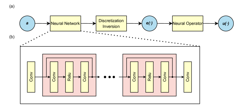
Figure 1: The upper panel shows the overall structure of our Fourier neural operator downscaling model denoted by $G_{\theta}$. The low-resolution input $\mathbf{a}$ goes through a neural network $f_{\theta}$ and a discretization inversion operator $T^{-1}$. Then an embedding function $\mathbf{e}(\cdot)$ over domain $D$ is returned. Finally, a neural operator $\mathcal{F}_{\theta}$ takes in $\mathbf{e}(\cdot)$ and outputs the target function $\mathbf{u}(\cdot)$ which interpolates the high-resolution observation of $\mathbf{a}$. The lower panel shows the detailed architecture of $f_{\theta}$, which starts and ends with a convolutional layer, sandwiching a series of convolutional residual blocks.

4 Experiments

4.1 Downscaling PDE Data

In order to evaluate the performance of our model to downscale PDE data, we used a dataset solving the 2D Navier-Stokes equation for a viscous and incompressible fluid in vorticity form (Li et al., 2021, Section 5.3). The equation was numerically solved $10000$ times at resolution $64\times 64$ with randomly sampled initial conditions. Each solution was integrated for $50$ time steps with a viscosity of $\text{10}^{-4}$. Out of $10000$ solutions, $7000$, $2000$, and $1000$ solutions were sampled as train, validation, and test sets, respectively. The solutions at each time step were then downsampled via average pooling to resolutions $32\times 32$ and $16\times 16$. Our PDE downscaling dataset consists of the solutions along with the downsampled versions.

Following implementation details specified in Section 3.2, we constructed our DFNO model and trained it on the PDE downscaling dataset with upsampling factor 2 (i.e., $16\times 16\rightarrow 32\times 32$), and then evaluated it at both 2 times (learned) and 4 times (zero-shot) downscaling.

As baselines for comparison, we trained two CNN (CNN-2 and CNN-4) and two GAN (GAN-2 and GAN-4) downscaling models with pre-defined upsampling factors 2 and 4. The network architectures follow the design in the paper by Harder et al. (2022b). The baseline models were trained on datasets of their corresponding upsampling factors, and their outputs were then adjusted to achieve the desired resolution for evaluation. Downscaling outputs from 2 times models (CNN-2 and GAN-2) increase their resoultion to 4 times by model recursion and bicubic interpolation. Correspondingly, downscaling outputs from 4 times models (CNN-4 and GAN-4) decrease their resolution to 2 times by average pooling and bicubic interpolation. As an additional simple, non-deep learning baseline, we also considered bicubic interpolation (de Boor, 1962) to the target resolution.

For reliable usage of downscaled results in downstream tasks, it is important for results to be both close to the ground truth and physically consistent. Harder et al. (2022b) showed that a softmax constraint layer can effectively enforce conservation laws in neural networks for downscaling, without decreasing accuracy. Thus, we conducted another set of experiments where all aforementioned models include an additional softmax constraint layer at its end to generate physically consistent outputs.

To evaluate each downscaling model, we computed the improvement with respect to the unconstrained bicubic baseline. In particular, in the case of error metrics, that is the mean squared error (MSE) and mean absolute error (MAE), the improvement was computed as the error of the bicubic baseline divided by the error of the evaluated model. In the case of the peak signal-to-noise ratio (PSNR) and the structural similarity index measure (SSIM), the improvement was computed as $100\times(M-B)/B$, where $B$ is the result of the bicubic baseline and $M$ is the result of the evaluated model. These derived relative results facilitate the comparison across models. These results are summarized visually in Figure 2 and we provide the evaluation numerical details in Tables 2, 4, 3, and 5.

In the unconstrained cases, DFNO shows dominant performance over all baseline models in all evaluation metrics for 2 times downscaling on which it was trained. This performance advantage persists when the DFNO model trained on 2 times downscaling is asked to zero-shot generalize to 4 times downscaling, where it outperforms models directly trained on the 4 times downscaling dataset such as CNN-4 and GAN-4. After the constraint layer is applied, DFNO’s skill is further boosted for both 2 times and 4 times downscaling. It is consistent with the conclusion by Harder et al. (2022b) that training networks with the constraint layer can introduce an inductive bias, helping networks give more accurate downscaling results. However, note that in the zero-shot downscaling cases where bicubic interpolation is used to adjust network output resolution (i.e., 4 times downscaling with CNN-2, 2 times downscaling with CNN-4, 4 times downscaling with GAN-2, and 2 times downscaling with GAN-4), the constraint layer generally degrades model performance. This is probably because these networks are not trained to adapt to the renormalization operation inside the constraint layer with a different upsampling factor.

One PDE solution downscaling example by our constrained DFNO model is presented in Figure 3. The top row shows the result of input reconstruction (1 time downscaling). Because of the softmax constraint layer, DFNO trivially reconstructs the exact input because the conservation law enforces the output to equal the input when the upsampling factor is 1. Rows 2 and 3 illustrate 2 times (learned) and 4 times (zero-shot) downscaling results by DFNO. In both cases, the downscaled outputs (column 1) are very close to the ground truth (column 2), and the difference (column 3) is minor and negligible with values roughly one order of magnitude lower than the ground truth values.

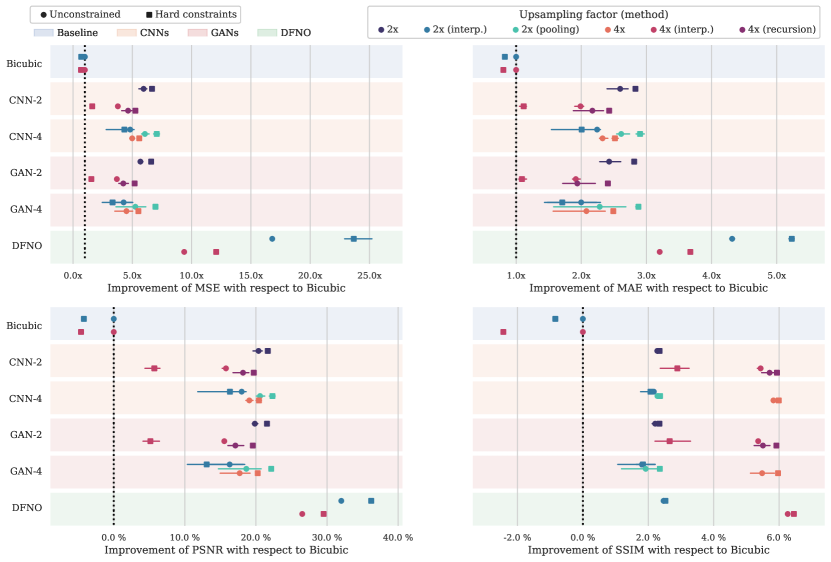
Figure 2: Metrics for downscaling models applied to the PDE dataset. Downscaling models CNN-2 (CNN-4) and GAN-2 (GAN-4) are trained with 2 times (4 times) downscaling data; the DFNO model is only trained with 2 times downscaling data. Each downscaling model is evaluated on both 2 times and 4 times downscaling. The 2 times downscaling outputs by CNN-2 and GAN-2 increase their resolution to 4 times through model recursion and bicubic interpolation. The 4 times downscaling outputs by CNN-4 and GAN-4 decrease their resolution to 2 times through average pooling and bicubic interpolation. Square (dot) denotes constrained (unconstrained) models. The metric mean and confidence interval from 3 runs are shown relatively to unconstrained bicubic interpolation. Model performance is evaluated by comparing marks of the same upsampling factor: cold colors for 2 times and warm colors for 4 times. Metric numerics and more details can be found in Tables 2, 4, 3, and 5.

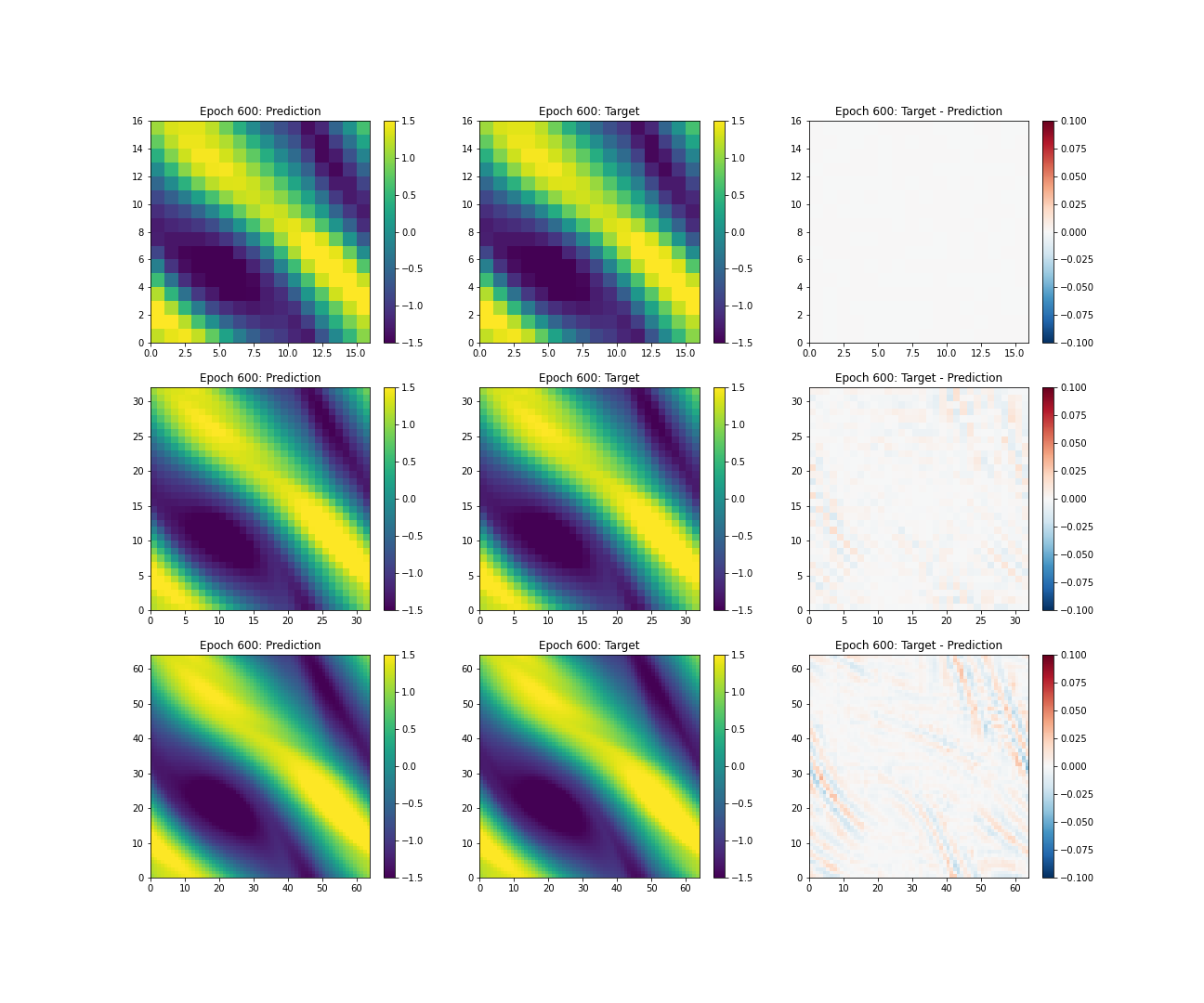
Figure 3: This figure shows the downscaling performance of our DFNO model with softmax constraint layer on the PDE solution data. The DFNO model was trained with 2 times downscaling data, then evaluated at 1 time (row 1), 2 times (row 2), and 4 times (row 3) downscaling. Column 1 shows the outputs from our DFNO model; column 2 is the numerical solution ground truth; and the difference (one order of magnitude lower than the ground truth values) between truth and prediction is presented in column 3.

4.2 Downscaling ERA5 Climate Data

The ERA5 climate and weather dataset (Hersbach et al., 2020) is a reanalysis product from the European Center for Medium-Range Weather Forecasts (ECMWF) that combines model data with worldwide observations. The observations are used as boundary conditions for numerical models that then predict various atmospheric variables. ERA5 is available as global hourly data with a $0.25^{\circ}\times 0.25^{\circ}$ resolution, which is roughly $25\leavevmode\nobreak\ \mbox{km}$ per pixel. It covers all years starting from 1950.

For this work, the quantity we focus on is the total column water that describes the vertical integral of the total amount of atmospheric water content, including water vapor, cloud water, and cloud ice but not precipitation. At each time step, we extract a random $128\times 128$ patch from the global water content field of size $721\times 1440$. There are roughly 60,000 time steps available in total. From these, 40,000 patches are randomly sampled for training and 10,000 for each validation and testing. The low-resolution counterparts are created by average pooling on high-resolution samples following the standard practice as in Serifi et al. (2021); Leinonen et al. (2021). It results in low-resolution samples of sizes $32\times 32$ and $64\times 64$. This operation is physically sound, considering that conservation of water content means that the water content (density per squared meter) described in a low-resolution pixel should be equal to the average of its corresponding high-resolution pixels.

As in the previous section, a DFNO model is trained with 2 times downscaling data and tested at 1 times, 2 times, and 4 times downscaling. Its performance is also compared against two CNN and two GAN downscaling models of upsampling factors 2 and 4. To enforce conservation law, a separate set of experiments are conducted with the softmax constraint layer applied. The downscaling performance of all models is collected in Tables 6 and 8 (without constraint layer) and Tables 7 and 9 (with constraint layer), and we provide a visualization of the relative improvement with respect to the bicubic baseline in Figure 4.

When the constraint layer is not applied, in learned (2 times) downscaling, we find that DFNO has the highest skill among all baseline models in all evaluation metrics. For zero-shot (4 times) downscaling, DFNO has an MAE score slightly worse than baseline CNN-2, CNN-4 and GAN-2 models but shows performance dominance in all the other metrics. Better performance in terms of MSE than MAE means the DFNO prediction errors mostly concentrate at values with magnitude less than 1. It is likely due to the fact that our DFNO is trained with MSE as the loss function, which is more sensitive to errors with large magnitude. After applying the constraint layer, DFNO performance in both learned and zero-shot downscaling is boosted showing performance dominance for all metrics.

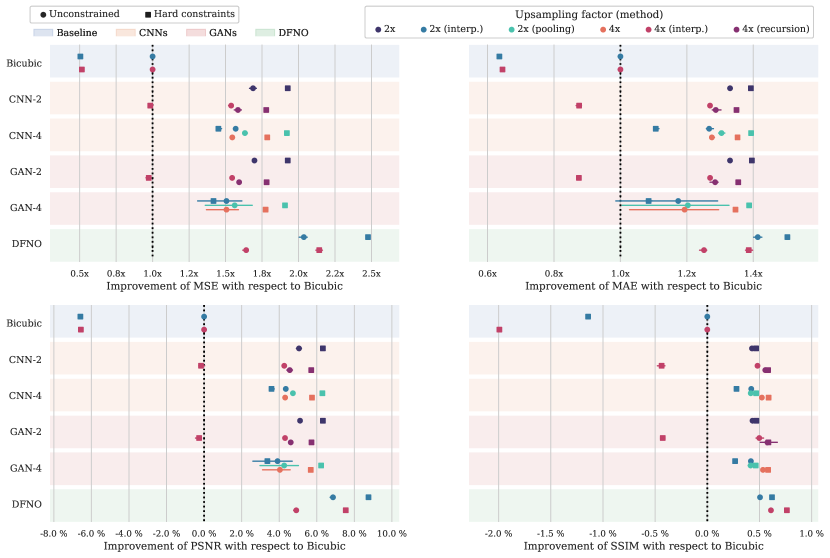
Figure 4: Metrics for downscaling models applied to the ERA5 dataset. Downscaling models CNN-2 (CNN-4) and GAN-2 (GAN-4) are trained with 2 times (4 times) downscaling data; the DFNO model is only trained with 2 times downscaling data. Each downscaling model is evaluated on both 2 times and 4 times downscaling. The 2 times downscaling outputs by CNN-2 and GAN-2 increase their resolution to 4 times through model recursion and bicubic interpolation. The 4 times downscaling outputs by CNN-4 and GAN-4 decrease their resolution to 2 times through average pooling and bicubic interpolation. Square (dot) denotes constrained (unconstrained) models. The metric mean and confidence interval from 3 runs are shown relatively to unconstrained bicubic interpolation. Model performance is evaluated by comparing marks of the same upsampling factor: cold colors for 2 times and warm colors for 4 times. Metric numerics and more details can be found in Tables 6, 8, 7, and 9.

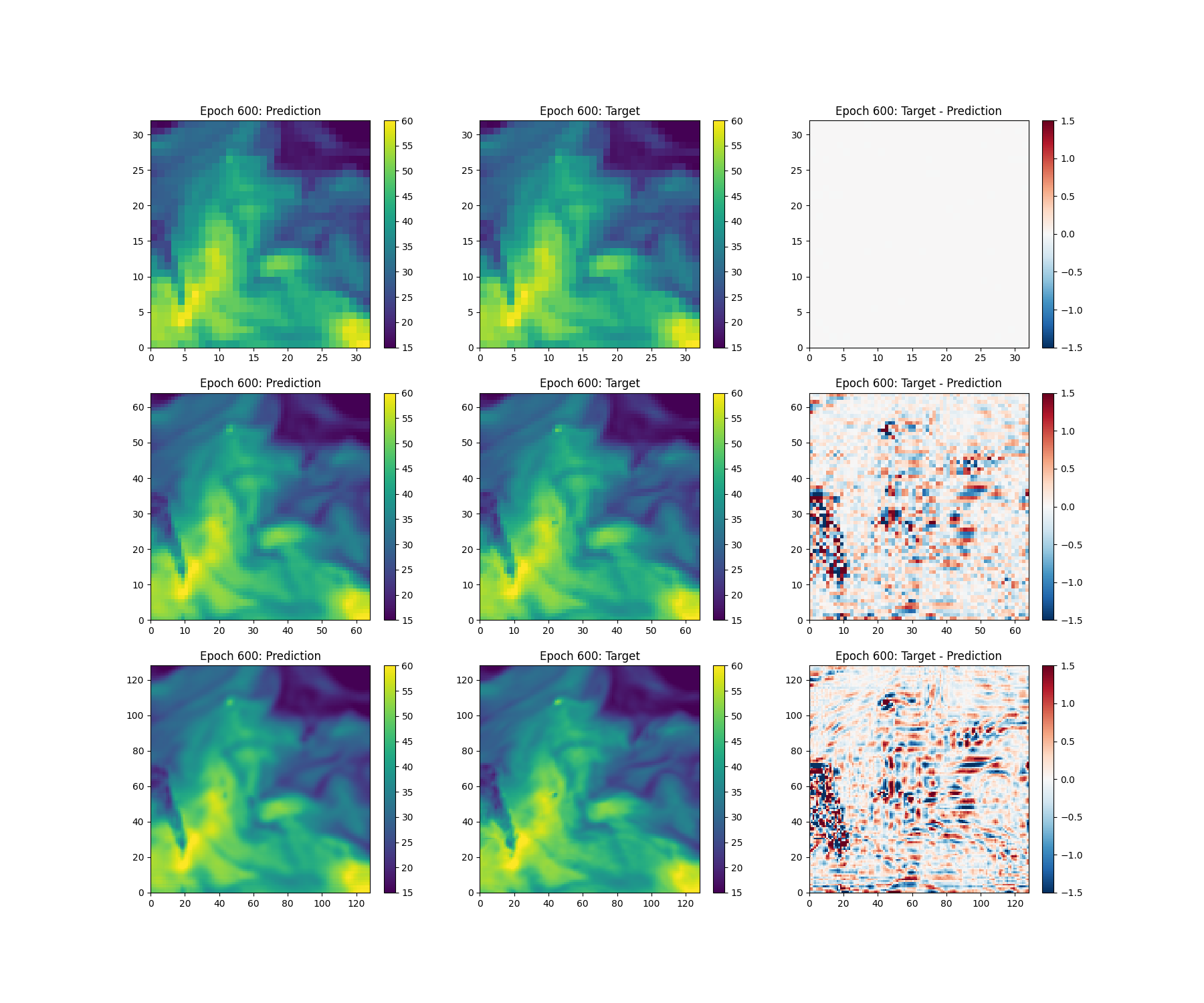
Figure 5: This figure shows the downscaling performance of our DFNO model with softmax constraint layer on ERA5 water content data. The DFNO model was trained with 2 times downscaling data, then evaluated at 1 time (row 1), 2 times (row 2), and 4 times (row 3) downscaling. Column 1 shows the outputs from our DFNO model; column 2 is the ground truth; the difference between truth and prediction is presented in column 3.

Figure 5 illustrates a case study on constrained DFNO downscaling ERA5 water content data. The softmax constraint layer helps DFNO reconstruct input perfectly (row 1). The 2 times downscaled (row 2) and 4 times downscaled (row 3) outputs are visually close to the ground truth (column 2) and with rather high perceptual quality as validated by quantitative metric scores in Tables 7 and 9. However, the error in column 3 is not as small as in the case of PDE solution downscaling (Figure 3). It is not surprising as our model is intended for PDE based climate simulation data downscaling rather than observational climate data downscaling; the FNO inside our model applies transformations on a truncated Fourier series, so it is naturally easier for it to model simulation data which have a more succinct representation in Fourier basis than observational data.

4.3 Downscaling for PDE Integration

This section considers the use of DFNO in integrating PDEs at high resolution (i.e., generating high resolution PDE solutions). There has been increasing interest in the use of data-driven deep learning-based methods to predict PDE solutions autoregressively (Li et al., 2021), and the Fourier neural operator was introduced as a state-of-the-art approach in this regard. Here, we show that the DFNO paradigm has the potential to significantly improve upon the standard FNO approach. Namely, we assume that we have access to an accurate low-resolution PDE solver, then use the DFNO to downscale the solution to higher resolution. Having a low-resolution PDE solution is a plausible assumption, since traditional numerical solvers are prohibitively time-intensive at high resolution but can be very cheap to run at low resolution.

Here we consider the Navier-Stokes equation as in Section 4.1. In the previous two sections, we have seen that the constrained DFNO outperforms the unconstrained DFNO; as a result, we here use only the constrained model. We train two different DFNO models, using 2 times ($16\times 16\rightarrow 32\times 32$) and 4 times ($16\times 16\rightarrow 64\times 64$) PDE downscaling data, respectively, and denoted as DFNO-2 and DFNO-4. We compare our approach against the standard FNO method, which predicts a solution one time step forward based on the solution at the previous ten time steps; two FNO models are trained with solution data at resolution $32\times 32$ and $64\times 64$, and are denoted as FFNO-32 and FFNO-64. Becasue FFNO-32 and FFNO-64 are resolution invariant, both of them are tested solving the Navier-Stokes equation at resolutions $32\times 32$ and $64\times 64$. In the end, all four models are evaluated with generated PDE solutions at resolutions $32\times 32$ and $64\times 64$.

The solutions generated by DFNO and FFNO models are compared against ground truth numerical solutions, and the performance is summarized in Table 1. Overall, DFNO models show a significant performance advantage over FFNO models. Comparing between DFNO models, it is not surprising that zero-shot downscaling is still not as good as learned downscaling. To evaluate DFNO and FFNO performance visually, solution examples generated by FFNO-64 and DFNO-2 at resolution $64\times 64$ for five consecutive time steps are presented in Figures 6 and 7. The generated solutions (column 1) are very close to numerical solutions (column 2) for both models. On the other hand, even though DFNO-2 zero-shot results are compared against FFNO-64 learned results, the error magnitude by DFNO-2 (column 3) is much less than that by FFNO-64. Results from both quantitative metric scores and visual illustration demonstrate that downscaling low-resolution solutions from numerical solvers gives better accuracy than generating by data-driven high-resolution solvers, that is, inputting low-resolution solutions as guidance makes it much easier to generate realistic high-resolution solutions.

Table 1: This table compares two ways of solving the Navier-Stokes equation at high resolution concerning mean squared error (MSE) and mean absolute error (MAE). First: solve the equation numerically at low resolution ($16\times 16$), then downscale the solution to $32\times 32$ and $64\times 64$ by constrained DFNO models. Second: use data-driven FFNO models to auto-regressively predict solutions at resolution $32\times 32$ and $64\times 64$.

Metric	Resolution	DFNO-2	DFNO-4	FFNO-32	FFNO-64
MSE	$32\times 32$	0.0004	0.0012	0.0101	0.0113
MSE	$64\times 64$	0.0018	0.0007	0.0136	0.0118
MAE	$32\times 32$	0.0124	0.0208	0.0677	0.0725
MAE	$64\times 64$	0.0246	0.0168	0.0788	0.0739

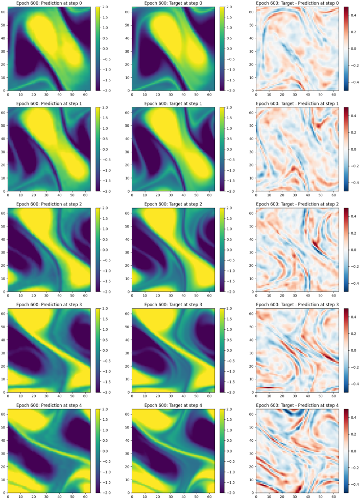
Figure 6: This figure shows Navier-Stokes equation solution $(64\times 64)$ at five consecutive time steps (row 1 to row 5). The solution is generated by FFNO-64, a forward solution prediction model trained on a solution dataset of resolution $64\times 64$. Column 1 shows FFNO-64 predicted solution; column 2 is the numerical solution ground truth; column 3 shows the difference between column 1 and column 2.

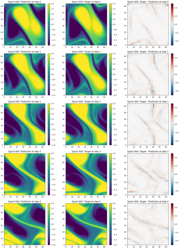
Figure 7: Similar to Figure 6 but the solution is generated by DFNO-2. It is a constrained DFNO model trained on solution downscaling data from $16\times 16$ to $32\times 32$. It performs zero-shot downscaling on a solution from $16\times 16$ to $64\times 64$.

5 Conclusion

In this work, we introduce the first arbitrary resolution downscaling model for climate data. This model takes in a low-resolution sample and outputs a function that interpolates the observed high-resolution counterpart. The low-resolution input is downscaled to an arbitrarily high resolution by evaluating the output function at discrete points. This model consists of three components: neural network, discretization inversion operator, and neural operator. They are implemented respectively as a residual convolutional network, bicubic interpolation, and a Fourier neural operator.

Our model is evaluated on a Navier-Stokes equation solution dataset and an ERA5 reanalysis water content dataset. It improves downscaling performance on both datasets significantly relative to state-of-the-art CNN and GAN super-resolution methods. It also zero-shot generalizes to higher upsampling factors, outperforming models directly trained on those factors. Our model’s performance is further boosted when a softmax constraint layer is applied to enforce conservation laws. Finally, we compare two ways to integrate PDEs at high resolution. Combining our downscaling model with a low-resolution numerical solver, the downscaled solution has superior accuracy to that of the state-of-the-art high-resolution data-driven solver.

While our DFNO approach conveys a significant performance improvement across all tasks, it demonstrates an even greater efficacy on climate simulation (Navier-Stokes equation) data as compared to observational climate (total water content) data. This may result from the fact that simulation data are much smoother than observational data; that is, simulation data have a more succinct representation in the Fourier basis than observational data. Therefore, simulation data are easier to be captured by a Fourier neural operator with a truncated Fourier series. It would be interesting to explore how to modify our model to adapt to data without a succinct Fourier representation so that its performance on observational climate data can be further improved.

Acknowledgments and Disclosure of Funding

This work was supported in part by the Québec Ministère de l’Économie et de l’Innovation, IBM, and the Canada CIFAR AI Chairs Program. The authors also acknowledge material support from NVIDIA in the form of computational resources, and are grateful for technical support from the Mila IDT team in maintaining the Mila Compute Cluster.

Appendix

Table 2: Downscaling performance on the PDE dataset in terms of mean squared error (MSE), mean absolute error (MAE), peak signal-to-noise ratio (PSNR), and structural similarity index measure (SSIM). The best scores are highlighted in bold red, second best in bold blue. The DFNO model was trained on 2 times downscaling data, then tested on 1 time, 2 times, and 4 times downscaling. CNN-2 (GAN-2) and CNN-4 (GAN-2) represent convolutional (generative adversarial) downscaling models with predefined upsampling factors 2 and 4. They were trained on datasets of their corresponding upsampling factors, whose downscaling results are then downsampled or upsampled via bicubic interpolation to get desired resolution for evaluation.

Metric	Factor	DFNO	CNN-2	CNN-4	GAN-2	GAN-4	Bicubic
MSE	$1\times$	0.0146	0.0057	0.0123	0.0056	0.0131	0.0000
MSE	$2\times$	0.0015	0.0042	0.0052	0.0044	0.0062	0.0252
MSE	$4\times$	0.0037	0.0093	0.0070	0.0095	0.0080	0.0350
MAE	$1\times$	0.0826	0.0524	0.0697	0.0520	0.0746	0.0000
MAE	$2\times$	0.0238	0.0397	0.0458	0.0424	0.0534	0.1027
MAE	$4\times$	0.0359	0.0579	0.0495	0.0601	0.0573	0.1150
PSNR	$1\times$	40.2750	44.3504	41.0302	44.4541	40.7810	154.0983
PSNR	$2\times$	50.2061	45.7778	44.8762	45.5806	44.2337	38.0326
PSNR	$4\times$	46.3361	42.4054	43.6083	42.3192	43.1123	36.6248
SSIM	$1\times$	0.9934	0.9968	0.9935	0.9963	0.9890	1.0000
SSIM	$2\times$	0.9981	0.9963	0.9952	0.9956	0.9917	0.9741
SSIM	$4\times$	0.9920	0.9842	0.9879	0.9835	0.9847	0.9335

Table 3: Similar to Table 2 but softmax constraint layer is applied to the output of each model.

Metric	Factor	DFNO	CNN-2	CNN-4	GAN-2	GAN-4	Bicubic
MSE	$1\times$	0.0000	0.0000	0.0000	0.0000	0.0000	0.0000
MSE	$2\times$	0.0011	0.0038	0.0063	0.0038	0.0084	0.0365
MSE	$4\times$	0.0029	0.0217	0.0063	0.0228	0.0064	0.0517
MAE	$1\times$	0.0000	0.0000	0.0000	0.0000	0.0000	0.0000
MAE	$2\times$	0.0196	0.0363	0.0528	0.0365	0.0627	0.1241
MAE	$4\times$	0.0313	0.1032	0.0457	0.1058	0.0462	0.1431
PSNR	$1\times$	151.8861	153.3908	152.4238	153.3476	152.1304	152.4239
PSNR	$2\times$	51.8071	46.2719	44.2463	46.2266	43.0041	36.4336
PSNR	$4\times$	47.4375	38.7146	44.1036	38.5096	44.0425	34.9377
SSIM	$1\times$	1.0000	1.0000	1.0000	1.0000	1.0000	1.0000
SSIM	$2\times$	0.9987	0.9969	0.9942	0.9969	0.9920	0.9659
SSIM	$4\times$	0.9937	0.9605	0.9894	0.9583	0.9892	0.9108

Table 4: Downscaling performance on the PDE dataset in terms of mean squared error (MSE), mean absolute error (MAE), peak signal-to-noise ratio (PSNR), and structural similarity index measure (SSIM). The best scores are highlighted in bold red, second best in bold blue. The DFNO model was trained on 2 times downscaling data, then tested on 1 time, 2 times, and 4 times downscaling. CNN-2 (GAN-2) and CNN-4 (GAN-2) represent convolutional (generative adversarial) downscaling models with predefined upsampling factors 2 and 4. They were trained on datasets of their corresponding upsampling factors, whose downscaling results are then downsampled (upsampled) via average pooling (model recursion) to get desired resolution for evaluation.

Metric	Factor	DFNO	CNN-2	CNN-4	GAN-2	GAN-4	Bicubic
MSE	$1\times$	0.0146	0.0002	0.0002	0.0004	0.0011	0.0000
MSE	$2\times$	0.0015	0.0042	0.0042	0.0044	0.0051	0.0252
MSE	$4\times$	0.0037	0.0076	0.0070	0.0083	0.0080	0.0350
MAE	$1\times$	0.0826	0.0097	0.0098	0.0164	0.0237	0.0000
MAE	$2\times$	0.0238	0.0397	0.0394	0.0424	0.0477	0.1027
MAE	$4\times$	0.0359	0.0535	0.0495	0.0600	0.0573	0.1150
PSNR	$1\times$	40.2750	60.8445	60.4059	56.6575	55.8089	154.0983
PSNR	$2\times$	50.2061	45.7778	45.8595	45.5806	45.1245	38.0326
PSNR	$4\times$	46.3361	43.2835	43.6083	42.8902	43.1123	36.6248
SSIM	$1\times$	0.9934	0.9996	0.9996	0.9989	0.9953	1.0000
SSIM	$2\times$	0.9981	0.9963	0.9963	0.9956	0.9928	0.9741
SSIM	$4\times$	0.9920	0.9868	0.9879	0.9849	0.9847	0.9335

Table 5: Similar to Table 4 but softmax constraint layer is applied to the output of each model.

Metric	Factor	DFNO	CNN-2	CNN-4	GAN-2	GAN-4	Bicubic
MSE	$1\times$	0.0000	0.0000	0.0000	0.0000	0.0000	0.0000
MSE	$2\times$	0.0011	0.0038	0.0036	0.0038	0.0036	0.0365
MSE	$4\times$	0.0029	0.0067	0.0063	0.0067	0.0064	0.0517
MAE	$1\times$	0.0000	0.0000	0.0000	0.0000	0.0000	0.0000
MAE	$2\times$	0.0196	0.0363	0.0354	0.0365	0.0357	0.1241
MAE	$4\times$	0.0313	0.0474	0.0457	0.0478	0.0462	0.1431
PSNR	$1\times$	151.8861	149.9829	147.8327	149.3479	147.5434	152.4239
PSNR	$2\times$	51.8071	46.2719	46.5235	46.2266	46.4569	36.4336
PSNR	$4\times$	47.4375	43.8382	44.1036	43.7889	44.0425	34.9377
SSIM	$1\times$	1.0000	1.0000	1.0000	1.0000	1.0000	1.0000
SSIM	$2\times$	0.9987	0.9969	0.9971	0.9969	0.9970	0.9659
SSIM	$4\times$	0.9937	0.9889	0.9894	0.9887	0.9892	0.9108

Table 6: Downscaling performance on the ERA5 water content dataset in terms of mean squared error (MSE), mean absolute error (MAE), peak signal-to-noise ratio (PSNR), and structural similarity index measure (SSIM). The best scores are highlighted in bold red, second best in bold blue. The DFNO model was trained on 2 times downscaling data, then tested on 1 time, 2 times, and 4 times downscaling. CNN-2 (GAN-2) and CNN-4 (GAN-2) represent convolutional (generative adversarial) downscaling models with predefined upsampling factors 2 and 4. They were trained on datasets of their corresponding upsampling factors, whose downscaling results are then downsampled or upsampled via bicubic interpolation to get desired resolution for evaluation.

Metric	Factor	DFNO	CNN-2	CNN-4	GAN-2	GAN-4	Bicubic
MSE	$1\times$	0.2140	0.0940	0.1566	0.0930	0.1752	0.0000
MSE	$2\times$	0.2063	0.2488	0.2677	0.2474	0.2815	0.4201
MSE	$4\times$	0.3628	0.3870	0.3851	0.3853	0.3970	0.5954
MAE	$1\times$	0.2896	0.1737	0.2149	0.1731	0.2439	0.0000
MAE	$2\times$	0.2392	0.2541	0.2668	0.2541	0.2920	0.3380
MAE	$4\times$	0.3067	0.3023	0.3010	0.3022	0.3251	0.3838
PSNR	$1\times$	46.9630	50.5294	48.3152	50.5795	47.8863	173.5160
PSNR	$2\times$	48.1002	47.2860	46.9688	47.3110	46.7714	45.0115
PSNR	$4\times$	46.0154	45.7349	45.7560	45.7535	45.6334	43.8633
SSIM	$1\times$	0.9964	0.9982	0.9971	0.9982	0.9971	1.0000
SSIM	$2\times$	0.9941	0.9933	0.9933	0.9934	0.9932	0.9891
SSIM	$4\times$	0.9895	0.9882	0.9886	0.9884	0.9887	0.9835

Table 7: Similar to Table 6 but softmax constraint layer is applied to the output of each model.

Metric	Factor	DFNO	CNN-2	CNN-4	GAN-2	GAN-4	Bicubic
MSE	$1\times$	0.0000	0.0000	0.0000	0.0000	0.0000	0.0000
MSE	$2\times$	0.1696	0.2181	0.2896	0.2181	0.2964	0.8314
MSE	$4\times$	0.2779	0.6054	0.3334	0.6118	0.3355	1.1552
MAE	$1\times$	0.0000	0.0000	0.0000	0.0000	0.0000	0.0000
MAE	$2\times$	0.2250	0.2427	0.3055	0.2422	0.3116	0.5318
MAE	$4\times$	0.2768	0.4383	0.2837	0.4386	0.2851	0.5950
PSNR	$1\times$	164.1793	170.2039	166.2301	169.6977	165.4083	161.0459
PSNR	$2\times$	48.9508	47.8584	46.6269	47.8584	46.5268	42.0471
PSNR	$4\times$	47.1723	43.7915	46.3820	43.7464	46.3549	40.9850
SSIM	$1\times$	1.0000	1.0000	1.0000	1.0000	1.0000	1.0000
SSIM	$2\times$	0.9952	0.9937	0.9919	0.9938	0.9917	0.9778
SSIM	$4\times$	0.9910	0.9792	0.9893	0.9793	0.9892	0.9639

Table 8: Downscaling performance on the ERA5 water content dataset in terms of mean squared error (MSE), mean absolute error (MAE), peak signal-to-noise ratio (PSNR), and structural similarity index measure (SSIM). The best scores are highlighted in bold red, second best in bold blue. The DFNO model was trained on 2 times downscaling data, then tested on 1 time, 2 times, and 4 times downscaling. CNN-2 (GAN-2) and CNN-4 (GAN-2) represent convolutional (generative adversarial) downscaling models with predefined upsampling factors 2 and 4. They were trained on datasets of their corresponding upsampling factors, whose downscaling results are then downsampled (upsampled) via average pooling (model recursion) to get desired resolution for evaluation.

Metric	Factor	DFNO	CNN-2	CNN-4	GAN-2	GAN-4	Bicubic
MSE	$1\times$	0.2140	0.0030	0.0046	0.0028	0.0243	0.0000
MSE	$2\times$	0.2063	0.2488	0.2573	0.2474	0.2713	0.4201
MSE	$4\times$	0.3628	0.3757	0.3851	0.3737	0.3970	0.5954
MAE	$1\times$	0.2896	0.0345	0.0440	0.0339	0.1087	0.0000
MAE	$2\times$	0.2392	0.2541	0.2592	0.2541	0.2852	0.3380
MAE	$4\times$	0.3067	0.2982	0.3010	0.2987	0.3251	0.3838
PSNR	$1\times$	46.9630	65.5137	63.8092	65.8671	59.5288	173.5160
PSNR	$2\times$	48.1002	47.2860	47.1402	47.3110	46.9310	45.0115
PSNR	$4\times$	46.0154	45.8635	45.7560	45.8862	45.6334	43.8633
SSIM	$1\times$	0.9964	1.0000	0.9999	1.0000	0.9998	1.0000
SSIM	$2\times$	0.9941	0.9933	0.9932	0.9934	0.9932	0.9891
SSIM	$4\times$	0.9895	0.9890	0.9886	0.9892	0.9887	0.9835

Table 9: Similar to Table 8 but softmax constraint layer is applied to the output of each model.

Metric	Factor	DFNO	CNN-2	CNN-4	GAN-2	GAN-4	Bicubic
MSE	$1\times$	0.0000	0.0000	0.0000	0.0000	0.0000	0.0000
MSE	$2\times$	0.1696	0.2181	0.2188	0.2181	0.2202	0.8314
MSE	$4\times$	0.2779	0.3347	0.3334	0.3343	0.3355	1.1552
MAE	$1\times$	0.0000	0.0000	0.0000	0.0000	0.0000	0.0000
MAE	$2\times$	0.2250	0.2427	0.2426	0.2422	0.2436	0.5318
MAE	$4\times$	0.2768	0.2844	0.2837	0.2833	0.2851	0.5950
PSNR	$1\times$	164.1793	155.5239	153.5080	155.0793	153.3323	161.0459
PSNR	$2\times$	48.9508	47.8584	47.8454	47.8584	47.8165	42.0471
PSNR	$4\times$	47.1723	46.3649	46.3820	46.3708	46.3549	40.9850
SSIM	$1\times$	1.0000	1.0000	1.0000	1.0000	1.0000	1.0000
SSIM	$2\times$	0.9952	0.9937	0.9937	0.9938	0.9937	0.9778
SSIM	$4\times$	0.9910	0.9892	0.9893	0.9893	0.9892	0.9639

References

- Balaji (2021) V. Balaji. Climbing down charney’s ladder: machine learning and the post-dennard era of computational climate science. Philosophical Transactions of the Royal Society A: Mathematical, Physical and Engineering Sciences, 379(2194):20200085, 2021. doi: 10.1098/rsta.2020.0085. URL https://royalsocietypublishing.org/doi/abs/10.1098/rsta.2020.0085.
- Ballas et al. (2015) N. Ballas, L. Yao, C. Pal, and A. Courville. Delving deeper into convolutional networks for learning video representations, 2015. URL https://arxiv.org/abs/1511.06432.
- Beucler et al. (2019) T. Beucler, S. Rasp, M. Pritchard, and P. Gentine. Achieving conservation of energy in neural network emulators for climate modeling, 2019. URL https://arxiv.org/abs/1906.06622.
- Beucler et al. (2021) T. Beucler, M. Pritchard, S. Rasp, J. Ott, P. Baldi, and P. Gentine. Enforcing analytic constraints in neural networks emulating physical systems. Physical Review Letters, 126(9), mar 2021. doi: 10.1103/physrevlett.126.098302. URL https://doi.org/10.1103%2Fphysrevlett.126.098302.
- Chaudhuri and Robertson (2020) C. Chaudhuri and C. Robertson. CliGAN: A structurally sensitive convolutional neural network model for statistical downscaling of precipitation from multi-model ensembles. Water, 12(12):3353, nov 2020. doi: 10.3390/w12123353. URL https://doi.org/10.3390%2Fw12123353.
- Chen et al. (2022) X. Chen, K. Feng, N. Liu, B. Ni, Y. Lu, Z. Tong, and Z. Liu. Rainnet: A large-scale imagery dataset and benchmark for spatial precipitation downscaling, 2022.
- Daw et al. (2020) A. Daw, R. Q. Thomas, C. C. Carey, J. S. Read, A. P. Appling, and A. Karpatne. Physics-guided architecture (PGA) of neural networks for quantifying uncertainty in lake temperature modeling. In Proceedings of the 2020 SIAM International Conference on Data Mining, pages 532–540. Society for Industrial and Applied Mathematics, jan 2020. doi: 10.1137/1.9781611976236.60. URL https://doi.org/10.1137%2F1.9781611976236.60.
- de Boor (1962) C. de Boor. Bicubic spline interpolation. Journal of Mathematics and Physics, 41(1-4):212–218, apr 1962. doi: 10.1002/sapm1962411212. URL https://doi.org/10.1002%2Fsapm1962411212.
- Dong et al. (2015) C. Dong, C. C. Loy, K. He, and X. Tang. Image super-resolution using deep convolutional networks, 2015. URL https://arxiv.org/abs/1501.00092.
- Goodfellow et al. (2014) I. J. Goodfellow, J. Pouget-Abadie, M. Mirza, B. Xu, D. Warde-Farley, S. Ozair, A. Courville, and Y. Bengio. Generative adversarial networks, 2014. URL https://arxiv.org/abs/1406.2661.
- Groenke et al. (2020) B. Groenke, L. Madaus, and C. Monteleoni. ClimAlign: Unsupervised statistical downscaling of climate variables via normalizing flows. In Proceedings of the 10th International Conference on Climate Informatics. ACM, sep 2020. doi: 10.1145/3429309.3429318. URL https://doi.org/10.1145%2F3429309.3429318.
- Harder et al. (2022a) P. Harder, D. Watson-Parris, P. Stier, D. Strassel, N. R. Gauger, and J. Keuper. Physics-informed learning of aerosol microphysics, 2022a. URL https://arxiv.org/abs/2207.11786.
- Harder et al. (2022b) P. Harder, Q. Yang, V. Ramesh, P. Sattigeri, A. Hernandez-Garcia, C. Watson, D. Szwarcman, and D. Rolnick. Generating physically-consistent high-resolution climate data with hard-constrained neural networks, 2022b. URL https://arxiv.org/abs/2208.05424.
- Harder et al. (2023) P. Harder, V. Ramesh, A. Hernandez-Garcia, Q. Yang, P. Sattigeri, D. Szwarcman, C. Watson, and D. Rolnick. Physics-constrained deep learning for climate downscaling, 2023.
- Hersbach et al. (2020) H. Hersbach, B. Bell, P. Berrisford, S. Hirahara, A. Horányi, J. Muñoz-Sabater, J. Nicolas, C. Peubey, R. Radu, D. Schepers, et al. The era5 global reanalysis. Quarterly Journal of the Royal Meteorological Society, 146(730):1999–2049, 2020.
- Höhlein et al. (2020) K. Höhlein, M. Kern, T. Hewson, and R. Westermann. A comparative study of convolutional neural network models for wind field downscaling. Meteorological Applications, 27(6), nov 2020. doi: 10.1002/met.1961. URL https://doi.org/10.1002%2Fmet.1961.
- Kasim et al. (2021) M. F. Kasim, D. Watson-Parris, L. Deaconu, S. Oliver, P. Hatfield, D. H. Froula, G. Gregori, M. Jarvis, S. Khatiwala, J. Korenaga, J. Topp-Mugglestone, E. Viezzer, and S. M. Vinko. Building high accuracy emulators for scientific simulations with deep neural architecture search. Machine Learning: Science and Technology, 3(1):015013, dec 2021. doi: 10.1088/2632-2153/ac3ffa. URL https://dx.doi.org/10.1088/2632-2153/ac3ffa.
- Kovachki et al. (2023) N. Kovachki, Z. Li, B. Liu, K. Azizzadenesheli, K. Bhattacharya, A. Stuart, and A. Anandkumar. Neural operator: Learning maps between function spaces, 2023.
- Leinonen et al. (2021) J. Leinonen, D. Nerini, and A. Berne. Stochastic super-resolution for downscaling time-evolving atmospheric fields with a generative adversarial network. IEEE Transactions on Geoscience and Remote Sensing, 59(9):7211–7223, sep 2021. doi: 10.1109/tgrs.2020.3032790. URL https://doi.org/10.1109%2Ftgrs.2020.3032790.
- Li et al. (2020) Z. Li, N. Kovachki, K. Azizzadenesheli, B. Liu, K. Bhattacharya, A. Stuart, and A. Anandkumar. Neural operator: Graph kernel network for partial differential equations, 2020. URL https://arxiv.org/abs/2003.03485.
- Li et al. (2021) Z. Li, N. B. Kovachki, K. Azizzadenesheli, B. liu, K. Bhattacharya, A. Stuart, and A. Anandkumar. Fourier neural operator for parametric partial differential equations. In International Conference on Learning Representations, 2021. URL https://openreview.net/forum?id=c8P9NQVtmnO.
- Liu et al. (2017) Z. Liu, R. A. Yeh, X. Tang, Y. Liu, and A. Agarwala. Video frame synthesis using deep voxel flow. In 2017 IEEE International Conference on Computer Vision (ICCV). IEEE, oct 2017. doi: 10.1109/iccv.2017.478. URL https://doi.org/10.1109%2Ficcv.2017.478.
- McCoy et al. (2020) I. L. McCoy, D. T. McCoy, R. Wood, L. Regayre, D. Watson-Parris, D. P. Grosvenor, J. P. Mulcahy, Y. Hu, F. A.-M. Bender, P. R. Field, et al. The hemispheric contrast in cloud microphysical properties constrains aerosol forcing. Proceedings of the National Academy of Sciences, 117(32):18998–19006, 2020.
- Price and Rasp (2022) I. Price and S. Rasp. Increasing the accuracy and resolution of precipitation forecasts using deep generative models, 2022. URL https://arxiv.org/abs/2203.12297.
- Serifi et al. (2021) A. Serifi, T. Günther, and N. Ban. Spatio-temporal downscaling of climate data using convolutional and error-predicting neural networks. Frontiers in Climate, 3, apr 2021. doi: 10.3389/fclim.2021.656479. URL https://doi.org/10.3389%2Ffclim.2021.656479.
- Tran et al. (2021) H. Tran, E. Leonarduzzi, L. D. la Fuente, R. B. Hull, V. Bansal, C. Chennault, P. Gentine, P. Melchior, L. E. Condon, and R. M. Maxwell. Development of a deep learning emulator for a distributed groundwater–surface water model: ParFlow-ML. Water, 13(23):3393, dec 2021. doi: 10.3390/w13233393. URL https://doi.org/10.3390%2Fw13233393.
- Wang et al. (2018) X. Wang, K. Yu, S. Wu, J. Gu, Y. Liu, C. Dong, C. C. Loy, Y. Qiao, and X. Tang. Esrgan: Enhanced super-resolution generative adversarial networks, 2018. URL https://arxiv.org/abs/1809.00219.
- Watson et al. (2020) C. D. Watson, C. Wang, T. Lynar, and K. Weldemariam. Investigating two super-resolution methods for downscaling precipitation: Esrgan and car, 2020. URL https://arxiv.org/abs/2012.01233.
- Watson-Parris (2021) D. Watson-Parris. Machine learning for weather and climate are worlds apart. Philosophical Transactions of the Royal Society A: Mathematical, Physical and Engineering Sciences, 379(2194):20200098, feb 2021. doi: 10.1098/rsta.2020.0098. URL https://doi.org/10.1098%2Frsta.2020.0098.