Robust non-computability and stability of dynamical systems

Abstract

In this paper, we examine the relationship between the stability of the dynamical system $x^{\prime}=f(x)$ and the computability of its basins of attraction. We present a computable $C^{\infty}$ system $x^{\prime}=f(x)$ that possesses a computable and stable equilibrium point, yet whose basin of attraction is robustly non-computable in a neighborhood of $f$ in the sense that both the equilibrium point and the non-computability of its associated basin of attraction persist when $f$ is slightly perturbed. This indicates that local stability near a stable equilibrium point alone is insufficient to guarantee the computability of its basin of attraction. However, we also demonstrate that the basins of attraction associated with a structurally stable - globally stable - planar system are computable. Our findings suggest that the global stability of a system plays a pivotal role in determining the computability of its basins of attraction.

1 Introduction

The focus of this paper is on examining the relationship between the stability of the dynamical system

$$\frac{dx}{dt}=f(x)$$ (1)

and the feasibility of computing the basin of attraction of a (hyperbolic) equilibrium point.

The problem of computing the basin of attraction of an equilibrium point can be viewed as a continuous variation of the discrete Halting problem. In this paper, we will demonstrate that basins of attraction can exhibit robust non-computability for computable systems. Specifically, we will present a computable system represented by Equation (1) and a neighborhood surrounding function $f$ which have the following properties: (i) Equation (1) has a computable equilibrium point, say $s_{f}$, and the basin of attraction of $s_{f}$ is non-computable; (ii) there are infinitely many computable functions within this neighborhood; and (iii) for each and every computable function $g$ in this neighborhood, the system described by $x^{\prime}=g(x)$ possesses a computable equilibrium point (near $s_{f}$) whose basin of attraction is also non-computable. To the best of our knowledge, this is the first instance where a continuous problem is demonstrated to possess robust non-computability.

Equilibrium solutions, also known as equilibrium points or critical points, correspond to the zeros of $f$ in (1) and play a vital role in dynamical systems theory. They are points where the system comes to rest and are useful in determining the stability of the system. By analyzing the system’s behavior in the vicinity of an equilibrium point, we can ascertain whether nearby trajectories (i.e. solutions of (1)) will remain near that point (stable) or move away from it (unstable).

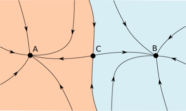
Figure 1: Example of a dynamical system having three equilibrium points $A,B,C$. The points $A$ and $B$ are sinks (i.e. stable equilibrium points) while $C$ is not (it is a so-called saddle equilibrium point). The region in orange is the basin of attraction of $A$ while the region in blue is the basin of attraction of $B$.

The basins of attraction, on the other hand, represent the collection of initial conditions with the property that their associated trajectories converge to the corresponding equilibrium point. This is pictured in Figure 1. Thus, by identifying the basins of attraction, we can predict the system’s long-term behavior for different initial conditions. This information is essential in understanding and characterizing the system’s behavior, particularly in the context of complex systems.

A sink of (1) is a special type of equilibrium point where the system in the neighborhood of the equilibrium point is well-behaved and stable. Here “stable” refers to at least two properties. First, each sink $s$ has a neighborhood $U$ with the property that any trajectory that enters $U$ stays there and converges exponentially fast to $s$ (this means that $\|\phi_{t}(x)-x_{0}\|\leq\varepsilon e^{-\alpha t}$ for some $\varepsilon,\alpha>0$, where $\phi_{t}(x)$ denotes the solution of (1) at time $t\geq 0$ with initial condition $\phi_{0}(x)=x\in U$. See [Per01, Theorem 1 on p. 130]). Second, the system is stable in the sense that if we replace $f$ in (1) by a nearby function $\overline{f}$ then it will continue to have a unique sink $\overline{s}$ in $U$ ($\overline{s}$ depends continuously on $\overline{f}$. In particular, when $\overline{f}=f$ one has $s=\overline{s}$. See [Per01, Theorem 1 on p. 321]) and moreover trajectories of the new system will behave (near the sink) similarly to the trajectories of the original system (1) and will converge exponentially fast to $\overline{s}$.

This means that if the system (1) is slightly perturbed from a sink, it will eventually return to that point. In other words, a sink point is robust locally under small perturbations. Moreover, even if the dynamics of the system is (slightly) perturbed, nearby trajectories will behave similarly to the original system, providing a better understanding of the long-term behavior of the system. This is particularly important in the study of complex systems, where the stability of the system can be difficult to determine analytically. The concept of robustness also allows for the development of numerical methods for the study of dynamical systems, which are crucial in many applications where analytical methods are not feasible.

The widespread use of numerical algorithms in the analysis of dynamical systems has made it crucial to determine which sets associated with a system can be computed, and which ones cannot. In essence, a set is computable if it can be accurately plotted or numerically described to any desired degree of precision. Equilibrium points and basins of attraction are examples of such sets.

Several studies [Zho09], [GZ15] revealed that the basin of attraction of a sink may not be computable, even if the system is analytic and computable, and the sink is computable. Furthermore, non-computability results are not restricted only to basins of attraction for differential equations (see e.g. [PER79], [PER81], [PEZ97], [GZB09], [GBC09], [GZB12], [BP20], [CMPSP21], [CMPS21]). These discoveries highlight the need to understand the limitations of numerical methods in the analysis of dynamical systems. In particular, it raises the question of whether non-computability results are “typical” or if they represent “exceptional” scenarios that are unlikely to have practical significance. In this paper, we specifically concentrate on investigating the non-computability of basins of attractions, as this phenomenon can be viewed as a continuous-time counterpart to the halting problem.

Moreover, it’s worth noting that numerical computations have finite precision, and hyperbolic sinks are robust under small perturbations. As a result, it’s worth considering if the non-computability remains under small perturbations. If it does not, the non-computability may be ignored in physical realities. In this paper, we show that the non-computability in computing the basin of attraction cannot be overlooked in the sense that the non-computability is robust under small perturbations. The following is our first main result (the precise statement is presented in section 3).

$\mathbf{Theorem\,1.}$ There exists a computable $C^{\infty}$ function $f$ for which the system (1) possesses a computable sink $s_{0}$, but the basin of attraction of $s_{0}$ is non-computable. Moreover, this non-computability is robust and persists under small perturbations.

It is worth noting that Theorem 1 establishes that local stability in the vicinity of a sink is insufficient to guarantee the computability of the basin of attraction at the sink.

We also provide a discrete-time variant of this theorem. Actually, this result will be proved first and then used to prove Theorem 1.

$\mathbf{Theorem\,2.}$ There exists an analytic and computable function $f$ for which the discrete-time dynamical system defined by the iteration of $f$ possesses a computable sink $s_{0}$, but the basin of attraction of $s_{0}$ is non-computable. Moreover, this non-computability is robust and persists under small perturbations.

The third main theorem of the paper provides an answer to the question of which dynamical systems have computable basins of attraction in the plane $\mathbb{R}^{2}$. The precise statement of the following theorem is presented in section 4.

$\mathbf{Theorem\,3.}$ The map that links each structurally stable planar system to the set of basins of attraction of its sinks is computable.

This theorem provides a positive result that complements the non-computability result presented in the first main theorem. It implies that for the large class of structurally stable - globally stable - planar systems, it is possible to numerically compute the basins of attraction of their equilibrium points and periodic orbits. It is worth noting that the set of structurally stable planar systems defined on a compact disk $K$ forms an open and dense subset of the set of all planar ($C^{1}$-) dynamical systems defined on $K$.

Taken together, Theorems 1 and 3 demonstrate that global stability is a crucial element in determining the feasibility of numerically computing the basins of attraction of dynamical systems, at least in the case of ordinary differential equations.

2 Preliminaries

2.1 Computable analysis

Let $\mathbb{N},\mathbb{Z},\mathbb{Q}$, and $\mathbb{R}$ be the set of non-negative integers, integers, rational numbers, and real numbers, respectively. Assuming familiarity with the concept of computable functions defined on $\mathbb{N}$ with values in $\mathbb{Q}$, we note that there exist several distinct but equally valid approaches to computable analysis, dating back to the work of Grzegorczyk and Lacombe in the 1950s. For the purposes of this paper, we adopt the oracle Turing machine version presented in e.g. [Ko91].

Definition 1.

A rational-valued function $\phi:\mathbb{N}\to\mathbb{Q}$ is called an oracle for a real number $x$ if it satisfies $|\phi(m)-x|<2^{-m}$ for all $m$.

Definition 2.

Let $S$ be a subset of $\mathbb{R}$, and let $f:S\to\mathbb{R}$ be a real-valued function on $S$. Then $f$ is said to be computable if there is an oracle Turing Machine $M^{\phi}(n)$ such that the following holds. If $\phi$ is an oracle for $x\in S$, then for every $n\in\mathbb{N}$, $M^{\phi}(n)$ returns a rational number $q$ such that $|q-f(x)|<2^{-n}$.

The definition can be extended to functions defined on a subset of $\mathbb{R}^{d}$ with values in $\mathbb{R}^{l}$.

Definition 3.

Let $U$ be a bounded open subset of $\mathbb{R}^{d}$. Then $U$ is called computable if there are computable functions $a,b:\mathbb{N}\to\mathbb{Q}^{d}$ and $r,s:\mathbb{N}\to\mathbb{Q}$ such that the following holds: $U=\cup_{n=0}^{\infty}B(a(n),r(n))$ and $\{\overline{B(b(n),s(n))}\}_{n}$ lists all closed rational balls in $\mathbb{R}^{d}$ which are disjoint from $U$, where $B(a,r)=\{x\in\mathbb{R}^{d}\,:\,|x-a|<r\}$ is the open ball in $\mathbb{R}^{d}$ centered at $a$ with the radius $r$ and $\overline{B(a,r)}$ is the closure of $B(a,r)$.

By definition, a planar computable bounded open set can be rendered on a computer screen with arbitrary magnification. A closed subset $K$ of $\mathbb{R}^{d}$ is considered computable if its complement $\mathbb{R}^{d}\setminus K$ is a computable open subset of $\mathbb{R}^{d}$, or equivalently, if the distance function $d_{K}:\mathbb{R}^{d}\to\mathbb{R}$ defined as $d_{K}(x)=\inf_{y\in D}\|y-x\|$ is computable.

The concept of Turing computability can be extended to encompass a broader range of function spaces and the maps that operate on them. The definitions 2 and 3 indicate that an object is deemed (Turing) computable if it can be approximated with arbitrary precision through computer-generated approximations. Formalizing this idea to carry out computations on infinite objects such as real numbers, we encode those objects as infinite sequences of rational numbers (or equivalently, sequences of any finite or countable set $\Sigma$ of symbols), using representations (see [Wei00] for a complete development). A represented space is a pair $(X;\delta)$ where $X$ is a set, $\delta$ is a coding system (or naming system) on $X$ with codes from $\Sigma$ having the property that $\mbox{dom}(\delta)\subseteq\Sigma^{\mathbb{N}}$ and $\delta:\Sigma^{\mathbb{N}}\to X$ is an onto map. Every $q\in\mbox{dom}(\delta)$ satisfying $\delta(q)=x$ is called a $\delta$-name of $x$ (or a name of $x$ when $\delta$ is clear from context). Naturally, an element $x\in X$ is computable if it has a computable name in $\Sigma^{\mathbb{N}}$. The notion of computability on $\Sigma^{\mathbb{N}}$ is well established, and $\delta$ lifts computations on $X$ to computations on $\Sigma^{\mathbb{N}}$. The representation $\delta$ also induces a topology $\tau_{\delta}$ on $X$, where $\tau_{\delta}=\{U\subseteq X:\,\delta^{-1}(U)\text{ is open in }\operatorname{dom}(\delta)\}$ is called the final topology of $\delta$ on $X$.

The notion of computable maps between represented spaces now arises naturally. A map $\Phi:(X;\delta_{X})\to(Y;\delta_{Y})$ between two represented spaces is computable if there is a computable map $\phi:\Sigma^{\mathbb{N}}\to\Sigma^{\mathbb{N}}$ such that $\Phi\circ\delta_{X}=\delta_{Y}\circ\phi$ as depicted below (see e.g. [BHW08]). Informally speaking, this means that there is a computer program $\phi$ that outputs a name of $\Phi(x)$ when given a name of $x$ as input. Since $\phi$ is computable, it transforms every computable element in $\Sigma^{\mathbb{N}}$ to a computable element in $\Sigma^{\mathbb{N}}$. Another fact about computable maps is that computable maps are continuous with respect to the corresponding final topologies induced by $\delta_{X}$ and $\delta_{Y}$.

2.2 Dynamical systems

There are two broad classes of dynamical systems: discrete-time and continuous-time. Discrete-time dynamical systems are defined by the iteration of a map $g:\mathbb{R}^{d}\rightarrow\mathbb{R}^{d}$, while continuous-time systems are defined by an ordinary differential equation (ODE) of the form $x^{\prime}=f(x)$, where $f:\mathbb{R}^{d}\rightarrow\mathbb{R}^{d}$. Regardless of the type of system, the notion of trajectory is fundamental. In the discrete-time case, a trajectory starting at the point $x_{0}$ is defined by the sequence of iterates of $g$ as follows

$$x_{0},g(x_{0}),g(g(x_{0})),\ldots,g^{[k]}(x_{0}),\ldots$$

where $g^{[k]}$ denotes the $k$th iterate of $g$, while in the continuous time case it is the solution, a function $\phi(f,x_{0})(\cdot)$ of time $t$, to the following initial-value problem

$$\left\{\begin{array}[c]{l}x^{\prime}=f(x)\\ x(0)=x_{0}\end{array}\right.$$

In the realm of dynamical systems, a set $A$ is considered forward invariant if any trajectory starting on $A$ remains on $A$ indefinitely for any positive time. If an invariant set consists of only one point, it is called an equilibrium point. For a dynamical system defined by (1), an equilibrium point must be a zero of $f$. Similarly, for a discrete-time dynamical system defined by $g$, an equilibrium point must be a fixed point of $g$ (i.e. it satisfies $g(x)=x$) or, equivalently, it must be a zero of $g(x)-x$.

If trajectories nearby an invariant set converge to this set, then the invariant set is called an attractor. The basin of attraction for a given attractor $A$ is the set of all points $x\in\mathbb{R}^{d}$ such that the trajectory starting at $x$ converges to $A$ as $t\rightarrow\infty$. Attractors come in different types, including points, periodic orbits, and strange attractors. Equilibrium points are the simplest type of attractor.

An equilibrium point $x_{0}$ of (1) is hyperbolic if none of the eigenvalues of the Jacobian matrix $Df(x_{0})$ have zero real part. In particular, if all the eigenvalues of $Df(x_{0})$ have a negative real part, then we are have a sink. A sink has all the properties mentioned in Section 1. In particular given a sink $s$ there is a neighborhood $U$ such that any trajectory starting in $U$ stays there and converges exponentially fast to $s$. If an hyperbolic equilibrium point is not a sink, then given any neighborhood of this point, there will be a trajectory that will never reach this equilibrium point.

A similar approach can be applied to discrete-time dynamical systems. Specifically, an equilibrium point $x_{0}$ of the discrete-time dynamical system defined by $g$ is hyperbolic if none of the eigenvalues of $Dg(x_{0})$ belong to the unit circle. On the other hand, an equilibrium point $x_{0}$ is considered a sink if all the eigenvalues of $Dg(x_{0})$ have an absolute value less than 1.

We will now discuss the concept of ($C^{1}$-)perturbations. First, we will introduce some notations. Let $C^{k}(A;\mathbb{R}^{l})$ denote the set of all $k$-times continuously differentiable functions from a subset $A$ of $\mathbb{R}^{d}$ to $\mathbb{R}^{l}$. If $l=d$, we simply write $C^{k}(A)$ for $C^{k}(A;\mathbb{R}^{d})$. Suppose $W$ is an open subset of $\mathbb{R}^{d}$ and $f:W\to\mathbb{R}^{d}$ is a $C^{1}$ vector field. In the field of dynamical systems and differential equations, a perturbation of $f$ is another $C^{1}$ vector field $g:W\to\mathbb{R}^{d}$ that is “$C^{1}$-close to $f$”. To be more precise:

Definition 4.

Let $f\in C(W)$ (resp. $f\in C^{1}(W)$), the $C$-norm of $f$ is defined to be $\|f\|=\sup_{x\in W}\|f(x)\|$ (resp. the $C^{1}$-norm of $f$ is defined to be $\|f\|_{1}=\sup_{x\in W}\|f(x)\|+\sup_{x\in W}\|Df(x)\|$), where $\|\cdot\|=$ denotes the max-norm on $\mathbb{R}^{d}$ or the usual norm of the matrix $Df(x)$, depending on the context.

Note that for $x\in\mathbb{R}^{d}$, the max-norm is given by $\|x\|=\max_{1\leq i\leq d}|x_{i}|$. It is possible that $\|f\|_{1}=\infty$ if the number is unbounded. The $C^{1}$-norm $\|\cdot\|_{1}$ has many of the same formal properties as norms for vector spaces. For $\epsilon>0$, an $\epsilon$-neighborhood of $f$ in $C^{1}(W)$ is defined as the set $\{g\in C^{1}(W):\|g-f\|_{1}<\epsilon\}$. Any function $g$ in this neighborhood is called an $\epsilon$-perturbation of $f$.

Remark 1.

Upon observation, it can be noted that for any function $f:W\rightarrow\mathbb{R}^{l}$, if $f$ is computable with a finite $\|f\|_{1}$, then in any $\epsilon$-neighborhood (in $C^{1}$-norm) $\mathcal{N}$, there exist infinitely many computable $C^{1}$ functions which are distinct from $f$. For example, $f_{\alpha},\bar{f}_{\alpha},\tilde{f}_{\alpha}\in\mathcal{N}$ for any rational $\alpha$ satisfying $0<\alpha<\epsilon$, where (the operations are done componentwise) $f_{\alpha}(x)=f(x)+\alpha$, $\bar{f}_{\alpha}(x)=f(x)+\alpha\sin x$, $\tilde{f}_{\alpha}(x)=f(x)+e^{-\alpha(1+\|x\|^{2})}$.

3 Proof of Theorem 2 – robust non-computability on the discrete-time case

In this section, we provide an example demonstrating the existence of a computable and analytic function $f:\mathbb{R}^{3}\rightarrow\mathbb{R}^{3}$ that defines a discrete-time dynamical system satisfying the following conditions:

1. $f$ has a hyperbolic sink $s$ that is computable.

2. The basin of attraction of $s$ is non-computable.

3. There exists a neighborhood $\mathcal{N}$ (in $C^{1}$-norm) of $f$ such that for every function $g\in\mathcal{N}$, $g$ has a hyperbolic sink $s_{g}$ that is computable from $g$, and the basin of attraction of $s_{g}$ is non-computable.

The construction demonstrates that the non-computability of computing the basins of attraction can remain robust under small perturbations and sustained throughout an entire neighborhood.

It is worth noting that the function $f$ inherits strong computability from its analyticity, which implies that every order derivative of $f$ is computable. Furthermore, in any $C^{1}$-neighborhood of $f$, there exist infinitely many computable functions.

We will make use of an example presented in [GZ15]. In [GZ15] an analytic and computable function $f:\mathbb{R}^{3}\to\mathbb{R}^{3}$ is explicitly constructed with the following properties:

• the restriction, $f_{M}:\mathbb{N}^{3}\to\mathbb{N}^{3}$, of $f$ on $\mathbb{N}^{3}$ is the transition function of a universal Turing machine $M$, where each configuration of $M$ is coded as an element of $\mathbb{N}^{3}$ (see [GZ15] for an exact description of the coding). Without loss of generality, $M$ can be assumed to have just one halting configuration; e.g. just before ending, clear the tape and go to a unique halting state; thus the halting configuration $s\in\mathbb{N}^{3}$ is unique. We also assume that $f_{M}$ is defined over $s$ and that $f(s)=s$.

• the halting configuration $s$ of $M$ is a computable sink of the discrete-time evolution of $f$.

• the basin of attraction of $s$ is non-computable.

• there exists a constant $\lambda\in(0,1)$ such that if $x_{0}$ is a configuration of $M$, then for any $x\in\mathbb{R}^{3}$,

  $$\|x-x_{0}\|\leq 1/4\quad\Longrightarrow\quad\|f(x)-f(x_{0})\|\leq\lambda\|x-x_{0}\|$$ (2)

In the remaining of this section, the symbols $f$ and $s$ are reserved for this particular function and its particular sink - the halting configuration of the universal Turing machine $M$ whose transition function is $f_{M}$.

We show in the following that there is a $C^{1}$-neighborhood $\mathcal{N}$ of $f$ – computable from $f$ and $Df(s)$ – such that for every $g\in\mathcal{N}$, $g$ has a sink $s_{g}$ – computable from $g$ – and the basin of attraction of $s_{g}$ is non-computable. We begin with two propositions. (Note that the particular function $f$ is exactly the function constructed in [GCB08] mentioned in the following proposition.)

Proposition 1.

([GCB08, p. 333]) Let $0<\delta<\epsilon<\frac{1}{2}$. The extension from $f_{M}:\mathbb{N}^{3}\to\mathbb{N}^{3}$ to $f:\mathbb{R}^{3}\to\mathbb{R}^{3}$ is robust to perturbations in the following sense: for all $g:\mathbb{R}^{3}\to\mathbb{R}^{3}$ such that $\|f-g\|\leq\delta$, for all $j\in\mathbb{N}$, and for all $\bar{x}_{0}\in\mathbb{R}^{3}$ satisfying $\|\bar{x}_{0}-x_{0}\|\leq\epsilon$, where $x_{0}\in\mathbb{N}^{3}$ represents an initial configuration,

$$\|g^{[j]}(\bar{x}_{0})-f_{M}^{[j]}(x_{0})\|\leq\epsilon$$ (3)

The following proposition is an immediate corollary of a classical result of dynamical systems theory. See e.g.  Theorems 1 and 2 in [HS74, p. 305]. The proof of this proposition has nothing to do with differential equations; rather, it depends on the invertibility of $Df(s)$ (the invertibility of $Df(s)$ follows from the fact that $s$ is a sink).

Proposition 2.

There exist a neighborhood $U\subset\mathbb{R}^{3}$ of $s$ and a $C^{1}$-neighborhood $\mathcal{N}$ of $f$ such that for any $g\in\mathcal{N}$, $g$ has a sink $s_{g}$ in $U$. Moreover, for any $\epsilon>0$ one can choose $\mathcal{N}$ so that $\|s_{g}-s\|<\epsilon$.

Remark 2.

We note that if $s$ is a sink of $f$, then $Df(s)-I$ is invertible, i.e. $\det(Df(s)-I)\neq 0$. Indeed, if $\det(Df(s)-I)=0$ then there would be a non-zero vector $v$ such that $(Df(s)-I)v=0$, a contradiction to the assumption that $s$ is a sink and thus that all eigenvalues of $Df(s)$ are less than 1 in absolute value. This implies that the sink $s$ is a zero of $h(x)=f(x)-x$ and that $Dh(s)$ is invertible (more generally, $Dh$ is invertible at any hyperbolic fixed point). Hence, if all fixed points of $f$ are hyperbolic, then one can compute globally the set of all zeros of $h(x)=f(x)-x$ (see[GZ21, Theorem 4.2]) and thus all fixed points of $f$. This implies that $s$ must be computable. One can then use the approach of [GZ21] or only use local information to compute the neighborhood $\mathcal{N}$ of Proposition 2. Indeed, with the aid of computable inverse function theorems such as those in [Zie06, Theorem 19] or [McN08, Corollary 6.1], a neighborhood $B(s,1/k_{0})$, where $k_{0}\in\mathbb{N}\setminus{0}$, can be computed from $f$, $Df$, and $s$ such that $f(x)-x$ is injective within this neighborhood. Consequently, there exists only one zero of $h(x)=f(x)-x$ in this vicinity, yielding a single fixed point of $f$. The sink $s$ can be computed as this zero with accuracy $1/k$, where $k\geq k_{0}$, by computing $h^{-1}(0)$ using the local inverse function $h^{-1}$ provided by the aforementioned computable inverse function theorems. As the computation is finite, the oracle call merely requires the use of a finite approximation of $h$, $Dh$, $f$, and $Df$ with an accuracy bounded by $1/\eta(k)$, where $\eta:\{k\in\mathbb{N}:,k\geq k_{0}\}\to\mathbb{N}$ (assuming $\eta(k)>k$ without loss of generality). Note that $\eta$ can be considered computable from $f$ and $Df$, for instance, by computing the sink $s$ with accuracy $1/k$ and measuring the maximum argument size used to call the oracle. By employing a similar argument to the one used to establish the computability of $s$ from $f$ and $Df$, one can demonstrate the computability of the function $F:\mathcal{N}\to\mathbb{R}^{3}$, where, for every $g\in\mathcal{N}$, $F(g)=s_{g}$, $s_{g}$ represents the unique equilibrium point of $g$ in the closure of $B(s,1/k_{0})$, and $\mathcal{N}$ denotes the $\frac{1}{\eta(k)}$-neighborhood (in $C^{1}$-norm) of $f$. Furthermore, $s_{g}$ is a sink and $|s-s_{g}|<1/k$.

Theorem 1.

There is a $C^{1}$-neighborhood $\mathcal{N}$ of $f$ (computable from $f$ and $Df(s)$) such that for any $g\in\mathcal{N}$, $g$ has a sink $s_{g}$ (computable from $g$) and the basin of attraction $W_{g}$ of $s_{g}$ is non-computable.

Proof.

Let $0<\delta<\epsilon<\frac{1}{2}$ be the parameters given in Proposition 1 satisfying $0<\epsilon<1/4$ and let $k_{0}$, $\eta$ be given as in Remark 2. Pick a $k\geq k_{0}$ such that $0<\frac{1}{k}<\epsilon/2$. Let $\theta$ be a rational constant satisfying $0<\theta<\min\{\delta,\frac{1-\lambda}{2},\frac{1}{\eta(k)}\}$, where $\lambda\in(0,1)$ is the constant in (2). Denote $\theta+\lambda$ as $\theta_{\lambda}$. Then $0<\theta_{\lambda}<\frac{1-\lambda}{2}+\lambda=\frac{1+\lambda}{2}<1$. Let $\mathcal{N}$ be the $\theta$-neighborhood of $f$ in $C^{1}$-norm. Then for any $g\in\mathcal{N}$, any configuration $x_{0}\in\mathbb{N}^{3}$ of $M$, and any $x\in B(x_{0},1/4)$, we have the following estimate:

$$\|g(x)-g(x_{0})\|$$ (4)

$$\leq \|(g-f)(x)-(g-f)(x_{0})\|+\|f(x)-f(x_{0})\|$$

$$\leq \|D(g-f)\|\,\|x-x_{0}\|+\lambda\|x-x_{0}\|$$

$$< (\theta+\lambda)\,\|x-x_{0}\|$$

Since $0<\theta+\lambda=\theta_{\lambda}<1$, it follows that $g$ is a contraction in $B(x_{0},1/4)$ for every configuration $x_{0}$ of $M$.

We now show that for any $g\in\mathcal{N}$ and any configuration $x_{0}\in\mathbb{N}^{3}$ of $M$, $M$ halts on $x_{0}$ if and only if $x_{0}\in W_{g}$, where $W_{g}$ denotes the basin of attraction of $s_{g}$. First we assume that $x_{0}\in W_{g}$. Then, by definition of basin of attraction of a sink, $g^{[j]}(x_{0})\to s_{g}$ as $j\to\infty$. Hence, there exists $n\in\mathbb{N}$ such that $\|g^{[n]}(x_{0})-s_{g}\|<\frac{\epsilon}{5}$, which in turn implies that

$$\|f_{M}^{[n]}(x_{0})-s\|$$

$$\leq \|f_{M}^{[n]}(x_{0})-g^{[n]}(x_{0})\|+\|g^{[n]}(x_{0})-s_{g}\|+\|s_{g}-s\|$$

$$\leq \epsilon+\frac{\epsilon}{5}+\frac{1}{k}<2\epsilon$$

Since $f_{M}^{[n]}(x_{0}),s\in\mathbb{N}^{3}$ and $2\epsilon<1/2$ by assumption that $\epsilon<\frac{1}{4}$, it follows that $f_{M}^{[n]}(x_{0})=s$. Hence, $M$ halts on $x_{0}$. Next we assume that $M$ halts on $x_{0}$. This assumption implies that there exists $n\in\mathbb{N}$ such that $f_{M}^{[j]}(x_{0})=s$ for all $j\geq n$. Then for all $j\geq n$, it follows from Proposition 1 that

$$\|g^{[j]}(x_{0})-s\|$$

$$\leq \|g^{[j]}(x_{0})-f_{M}^{[j]}(x_{0})\|+\|f_{M}^{[j]}(x_{0})-s\|$$

$$= \|g^{[j]}(x_{0})-f_{M}^{[j]}(x_{0})\|\leq\epsilon$$

The inequality implies that $\{g^{[j]}(x_{0})\}_{j\geq n}\subset\overline{B(s,\epsilon)}$. From the assumptions that $s_{g}$ is an equilibrium point of $g$, $\|s-s_{g}\|<\frac{1}{k}$ for every $g$ in the $\frac{1}{\eta(k)}$-neighborhood of $f$ (in $C^{1}$-norm), $\theta\leq\frac{1}{\eta(k)}$, and $\frac{1}{k}<\epsilon$, it follows that $g(s_{g})=s_{g}$ and $s_{g}\in\overline{B(s,\epsilon)}\subset\overline{B(s,1/4)}$. Since $s$ is a configuration of $M$ – the halting configuration of $M$ – it follows from (4) that $g$ is a contraction on $\overline{B(s,1/4)}$. Thus, $\|g^{[n+j]}(x_{0})-s_{g}\|=\|g^{[n+j]}(x_{0})-g^{[n+j]}(s_{g})\|\leq(\theta_{\lambda})^{j}\|g^{[n]}(x_{0})-s_{g}\|\to 0$ as $j\to\infty$. Consequently, $g^{[j]}(x_{0})\to s_{g}$ as $j\to\infty$, This implies that $x_{0}\in W_{g}$.

To prove that $W_{g}$ is non-computable, the following stronger inclusion is needed: if $M$ halts on $x_{0}$, then $B(x_{0},\epsilon)\subset W_{g}$. Consider any $x\in B(x_{0},\epsilon)$. Since $x_{0}\in W_{g}$ and $g$ is a contraction on $B(x_{0},\epsilon)$, it follows that

$$\|g^{[j]}(x)-g^{[j]}(x_{0})\|\leq(\theta_{\lambda})^{j}\|x-x_{0}\|\to 0\quad\mbox{as $j\to\infty$}$$

Since $x_{0}\in W_{g}$, $g^{[j]}(x_{0})\to s_{g}$ as $j\to\infty$. Hence, $g^{[j]}(x)\to s_{g}$ as $j\to\infty$. This implies that $x\in W_{g}$.

It remains to show that $W_{g}$ is non-computable. Suppose otherwise that $W_{g}$ was computable. We first note that $W_{g}=\cup_{t\in\mathbb{N}}\phi_{-t}(B(x_{0},\epsilon))$ is an open set since $\phi_{t}$ is continuous for every $t\in\mathbb{R}$ (this is a well-known fact that follows from the formula (20)) and furthermore $\phi_{t}^{-1}=\phi_{-t}$. Then the distance function $d_{\mathbb{R}^{3}\setminus W_{g}}$ is computable. We can use this computability to solve the halting problem. Consider any initial configuration $x_{0}\in\mathbb{N}^{3}$, and compute $d_{\mathbb{R}^{3}\setminus W_{g}}(x_{0})$. If $d_{\mathbb{R}^{3}\setminus W_{g}}(x_{0})>\frac{\epsilon}{5}$ or $d_{\mathbb{R}^{3}\setminus W_{g}}(x_{0})<\frac{\epsilon}{4}$, halt the computation. Since $\epsilon>0$, this computation always halts.

If $d_{\mathbb{R}^{3}\setminus W_{g}}(x_{0})>\frac{\epsilon}{5}>0$, then $x_{0}\in W_{g}$, or equivalently, the Turing machine $M$ halts on $x_{0}$. Otherwise, if $d_{\mathbb{R}^{3}\setminus W_{g}}(x_{0})<\frac{\epsilon}{4}$, then $x_{0}\not\in W_{g}$, or equivalently, $M$ does not halt on $x_{0}$. The exclusion that $x_{0}\not\in W_{g}$ is derived from the fact that if $x_{0}\in W_{g}$, then $B(x_{0},\epsilon)\subseteq W_{g}$; in other words, $d_{\mathbb{R}^{3}\setminus W_{g}}(x_{0})\geq\epsilon>\frac{\epsilon}{4}$. Therefore, if $W_{g}$ was computable, then we could solve the halting problem, which is a contradiction.

Hence, we conclude that $W_{g}$ is non-computable. ∎

Remark 3.

Theorem 1 demonstrates that non-computability can maintain its strength when considering standard topological structures, as in the study of natural phenomena such as identifying invariant sets of a dynamical system. This robustness can manifest in a powerful way: the non-computability of the basins of attraction persists continuously for every function that is “$C^{1}$ close to $f$”.

4 Proof of Theorem 1 – robust non-computability in the continuous-time case

In the previous section, we demonstrated that a discrete-time dynamical system defined by the iteration of a map, say $\bar{f}:\mathbb{R}^{3}\rightarrow\mathbb{R}^{3}$, has a computable sink with a non-computable basin of attraction, and that this non-computability property is robust to perturbations. In this section, we extend this result to continuous-time dynamical systems. Specifically, we prove the existence of a computable $C^{\infty}$ map $f:\mathbb{R}^{7}\rightarrow\mathbb{R}^{7}$ such that the ODE $y^{\prime}=f(y)$ has a computable sink with a non-computable basin of attraction. Moreover, this non-computability property is robust to small perturbations in $f$.

To be more precise, we show that there exists some $\varepsilon>0$ such that if $g:\mathbb{R}^{7}\rightarrow\mathbb{R}^{7}$ is another $C^{\infty}$ map with $\left\|f-g\right\|_{1}\leq\varepsilon$, then the ODE $y^{\prime}=g(y)$ also has a sink (computable from $g$ and located near the sink of $y^{\prime}=f(y)$) with a non-computable basin of attraction. This means that the non-computability of the basin of attraction is a robust property of the underlying dynamical system.

Overall, this result shows that the non-computability of basin of attraction is not limited to discrete-time dynamical systems, but is also present in continuous-time dynamical systems, and is a robust property that persists under small perturbations.

To obtain this result, we will employ a technique that involves iterating the map $\bar{f}$ with an ODE. We need to ensure that the resulting ODE still has a computable sink and that the non-computability property is robust to perturbations. This technique has been explored in several previous papers, including [CMC00], [CMC02], [GCB08], and [GZar]. The basic idea is to start with a “targeting” equation with the format

$$x^{\prime}=c(b-x)^{3}\phi(t)$$ (5)

where $b$ is the target value and $\phi:\mathbb{R}\mathbb{\rightarrow R}$ is a continuous function which satisfies $\int_{t_{0}}^{t_{1}}\phi(t)dt>0$ and $\phi(t)\geq 0$ over $[t_{0},t_{1}]$. This is a separable ODE which can be explicitly solved. Using the solution one can show that for any $\gamma>0$ (the value $\gamma$ is called the targeting error for reasons which will be clear in a moment), if one chooses

$$c\geq\frac{1}{2\gamma^{2}\int_{t_{0}}^{t_{1}}\phi(t)dt}$$ (6)

in (5), then $\left|x(t)-b\right|<\gamma$ for all $t\geq t_{1}$, independent of the initial condition $x(t_{0})$. Note also that if $\phi(t)=0$ for all $t\in[t_{0},t_{1}]$, then $x(t)=x(t_{0})$ for all $t\in[t_{0},t_{1}]$. This targeting equation is the basic construction block for iterating a map $\tilde{f}:\mathbb{R\rightarrow R}$, which extends a corresponding function $\tilde{f}_{\mathbb{N}}:\mathbb{N\rightarrow N}$.

To iterate $\tilde{f}$ (with an ODE) we pick $t_{1}-t_{0}=1/2$, a continuous periodic function $\phi:\mathbb{R\rightarrow R}$ of period 1, which satisfies $\phi(t)\geq 0$ for $t\in]0,1/2[$, $\phi(t)=0$ for $t\in[1/2,1]$, and $\int_{0}^{1}\phi(t)dt>0$, a constant $c$ satisfying (6) with $\gamma=1/4$, and a $C^{\infty}$ function $r:\mathbb{R\rightarrow R}$ with the property that $r(k+\varepsilon)=k$ for all $k\in\mathbb{Z}$ and all $0\leq\varepsilon\leq 1/4$ (i.e. $r$ returns the integer part of its argument $x$ whenever $x$ is within distance $\leq 1/4$ of an integer). Although the exact expressions of $\phi$ and $r$ are irrelevant to the construction, it is worth noticing that choices can be made (see e.g. [GCB08, p. 344], replacing $\theta_{j}$ in (20) of that paper by the function $\chi$ given by (11) below) so that $\phi$ and $r$ are $C^{\infty}$.

Then the ODE

$$\left\{\begin{array}[c]{l}z_{1}^{\prime}=c(\tilde{f}(r(z_{2}))-z_{1})^{3}\phi(t)\\ z_{2}^{\prime}=c(r(z_{1})-z_{2})^{3}\phi(t+1/2)\end{array}\right.$$ (7)

will iterate $\tilde{f}$ in the sense that the continuous flow generated by (7) starting near any integer value will stay close to the (discrete) orbit of $\tilde{f}$, as we will now see. Suppose that at the initial time $t=0$, we have $\left|z_{1}(0)-x_{0}\right|\leq 1/4$ and $\left|z_{2}(0)-x_{0}\right|\leq 1/4$ for some $x_{0}\in\mathbb{Z}$. During the first half-unit interval $[0,1/2]$, we have $\phi(t+1/2)=0$, and thus $z_{2}^{\prime}(t)=0$. Consequently, $z_{2}(t)=z_{2}(0)$, and hence $r(z_{2})=x_{0}$. Therefore, the first equation of (7) becomes a targeting equation (5) on the interval $[0,1/2]$ where the target is $\tilde{f}(r(z_{2}))=\tilde{f}(x_{0})$. Thus, we have $\left|z_{1}(1/2)-\tilde{f}(x_{0})\right|\leq 1/4$.

In the next half-unit interval $[1/2,1]$, the behavior of $z_{1}$ and $z_{2}$ switches. We have $\phi(t)=0$, and thus $z_{1}(t)=z_{1}(1/2)$, which implies that $r(z_{1})=\tilde{f}(x_{0})$. Hence, the second equation of (7) becomes a targeting equation (5) on the interval $[0,1/2]$ where the target is $r(z_{1})=\tilde{f}(x_{0})$. Thus, we have $\left|z_{2}(1)-\tilde{f}(x_{0})\right|\leq 1/4$.

In the next unit interval $[1,2]$, the same behavior repeats itself, so we have $\left|z_{1}(2)-\tilde{f}(\tilde{f}(x_{0}))\right|\leq 1/4$ and $\left|z_{2}(2)-\tilde{f}(\tilde{f}(x_{0}))\right|\leq 1/4$. In general, for any $k\in\mathbb{N}$ and $t\in[k,k+1/2]$, we will have $\left|z_{1}(k)-\tilde{f}^{[k]}(x_{0})\right|\leq 1/4$, $\left|z_{2}(k)-\tilde{f}^{[k]}(x_{0})\right|\leq 1/4$, and $\left|z_{2}(t)-\tilde{f}^{[k]}(x_{0})\right|\leq 1/4$. In other words, the flow of (7) starting near any integer value stays close to the orbit of $\tilde{f}$.

Notice also that by choosing $\gamma=1/8$ instead of $\gamma=1/4$, we can make (7) robust to perturbations of magnitude $\leq 1/8$, since under these conditions the system

$$\left\{\begin{array}[c]{l}\bar{z}_{1}^{\prime}=c(\tilde{f}(r(\bar{z}_{2}))-\bar{z}_{1})^{3}\phi(t)+\xi_{1}(t)\\ \bar{z}_{2}^{\prime}=c(r(\bar{z}_{1})-\bar{z}_{2})^{3}\phi(t+1/2)+\xi_{2}(t)\end{array}\right.$$ (8)

still satisfies the conditions $\left|z_{1}(k)-\tilde{f}^{[k]}(x_{0})\right|\leq 1/4$, $\left|z_{2}(k)-\tilde{f}^{[k]}(x_{0})\right|\leq 1/4$, and $\left|z_{2}(t)-\tilde{f}^{[k]}(x_{0})\right|\leq 1/4$ for all $k\in\mathbb{N}$ and $t\in[k,k+1/2]$, where $\left|\xi_{1}(t)\right|\leq 1/8$, $\left|\xi_{2}(t)\right|\leq 1/8$ for all $t\in\mathbb{R}$, and $\left|z_{1}(0)-x_{0}\right|\leq 1/8$, $\left|z_{2}(0)-x_{0}\right|\leq 1/8$. Indeed, in $[0,1/2]$ we have $\phi(t+1/2)=0$ and hence $\bar{z}_{2}^{\prime}=\xi_{2}(t)$ which yields $\left|z_{2}(t)-z_{2}(0)\right|\leq\int_{0}^{1/2}\left|\xi_{2}(t)\right|dt\leq(1/2)(1/8)=1/16$ and thus $\left|z_{2}(t)-x_{0}\right|\leq\left|z_{2}(t)-z_{2}(0)\right|+\left|z_{2}(0)-x_{0}\right|\leq 1/16+1/8=3/16$ for all $t\in[0,1/2]$. Therefore $\tilde{f}(r(\bar{z}_{2}))=\tilde{f}(x_{0})$ in $[0,1/2]$. Using an analysis similar to that performed in [GCB08, p. 346], where the “perturbed” targeting ODE

$$x^{\prime}=c(b-x)^{3}\phi(t)+\xi(t)\quad(\mbox{with $\left|\xi(t)\right|\leq\rho$})$$ (9)

is studied, we conclude that if $c$ satisfies (6), then $\left|x(t_{1})-b\right|<\gamma+\rho\cdot(t_{1}-t_{0})$. In the present case $t_{1}-t_{0}=1/2$ and $\rho=1/8$, and thus $\left|z_{1}(1/2)-\tilde{f}(x_{0})\right|\leq 1/8+(1/8)(1/2)=3/16$. Similarly, since $\phi(t)=0$, on $[1/2,1]$ we conclude that $\left|z_{1}(t)-\tilde{f}(x_{0})\right|\leq\left|z_{1}(1/2)-\tilde{f}(x_{0})\right|+\int_{1/2}^{1}\left|\xi_{2}(t)\right|dt\leq 3/16+(1/2)(1/8)=1/4$ for all $t\in[1/2,1]$. Therefore $r(\bar{z}_{1})=\tilde{f}(x_{0})$ in $[1/2,1]$ and thus $\left|z_{2}(1)-\tilde{f}(x_{0})\right|\leq 1/8+(1/8)(1/2)=3/16$. By repeating this procedure on subsequent intervals, we conclude that $\left|z_{1}(k)-\tilde{f}^{[k]}(x_{0})\right|\leq 1/4$, $\left|z_{2}(k)-\tilde{f}^{[k]}(x_{0})\right|\leq 1/4$ and $\left|z_{2}(t)-\tilde{f}^{[k]}(x_{0})\right|\leq 1/4$ for all $k\in\mathbb{N}$ and $t\in[k,k+1/2]$.

The above procedure can be readily extended to iterate (with an ODE) the three-dimensional map $\bar{f}:\mathbb{R}^{3}\rightarrow\mathbb{R}^{3}$ of the previous section by assuming that $\bar{f}=(\bar{f}_{1},\bar{f}_{2},\bar{f}_{3})$, where $\bar{f}_{i}:\mathbb{R}^{3}\rightarrow\mathbb{R}$ is a component of $\bar{f}$ for $i=1,2,3$. To accomplish this, it suffices to consider the ODE

$$\left\{\begin{array}[c]{l}u_{1}^{\prime}=c(\bar{f}_{1}(r(v_{1}),r(v_{2}),r(v_{3}))-u_{1})^{3}\phi(t)\\ u_{2}^{\prime}=c(\bar{f}_{2}(r(v_{1}),r(v_{2}),r(v_{3}))-u_{2})^{3}\phi(t)\\ u_{3}^{\prime}=c(\bar{f}_{3}(r(v_{1}),r(v_{2}),r(v_{3}))-u_{3})^{3}\phi(t)\\ v_{1}^{\prime}=c(r(u_{1})-v_{1})^{3}\phi(t+1/2)\\ v_{2}^{\prime}=c(r(u_{2})-v_{2})^{3}\phi(t+1/2)\\ v_{3}^{\prime}=c(r(u_{3})-v_{3})^{3}\phi(t+1/2)\end{array}\right.$$ (10)

This ODE works like (7), but applies componentwise to each component $\bar{f}_{1},\bar{f}_{2},\bar{f}_{3}$. However, a few problems still need to be addressed in order to achieve our desired results. Specifically, we must: (i) acquire an autonomous system of the form $y^{\prime}=f(y)$ rather than a non-autonomous one like (10), (ii) demonstrate the existence of a sink with a non-computable basin of attraction, and (iii) establish that both the sink and the non-computability of the basin of attraction are resilient to perturbations.

To address problem (i), one possible solution would be to introduce a new variable $z$ that satisfies $z^{\prime}=1$ and $z(0)=0$, effectively replacing $t$ in (10) with $z$. However, this approach would not be compatible with problem (ii) because the component $z$ would grow infinitely and never converge to a value, which is necessary for the existence of a sink.

One potential solution to this problem is to introduce a new variable $z$ such that $z(0)=0$ and $z^{\prime}=1$ until the Turing machine $M$ halts, and then set $z^{\prime}=-z$ afterwards so that the dynamics of $z$ converge to the sink at $0$ in one-dimensional dynamics. Since $z$ will replace $t$ as the argument of $\phi$ in (10), we also need to modify $\phi$ such that when $M$ halts, the components of $u=(u_{1},u_{2},u_{3})$ and $v=(v_{1},v_{2},v_{3})$ still converge to a sink that corresponds to the unique halting configuration of $M.$

In order to describe the dynamics of $z$, we first need to introduce several auxiliary tools. Consider the $C^{\infty}$ function $\chi$ defined by

$$\chi(x)=\left\{\begin{array}[c]{ll}0&\text{if }x\leq 0\text{ or }x\geq 1\\ e^{\frac{1}{x(x-1)}}\text{ \ \ }&\text{if }0<x<1.\end{array}\right.$$ (11)

Notice that $\chi$, as well as all its derivatives, is computable. Now consider the $C^{\infty}$ function $\zeta$ defined by $\zeta(0)=0$ and

$$\zeta^{\prime}(x)=c\chi(x)$$

where $c=\left(\int_{0}^{1}e^{\frac{1}{x(x-1)}}dx\right)^{-1}$, which is a $C^{\infty}$ version of Heaviside’s function (see also [Cam02, p. 4]) since $\zeta(x)=0$ when $x\leq 0$, $\zeta(x)=1$ when $x\geq 1$, and $0<\zeta(x)<1$ when $0<x<1$. Notice that $\zeta$ is computable since the solution of an ODE with computable data is computable [GZB09], [CG08], [CG09]. Similar properties are trivially obtained for the function $\zeta_{a,b}$, where $a<b$, defined by

$$\zeta_{a,b}(x)=\zeta\left(\frac{x-a}{b-a}\right)=\left\{\begin{array}[c]{ll}0&\text{if }x\leq a\\ \ast&\text{if }a<x<b\\ 1\text{ \ \ }&\text{if }x\geq b\end{array}\right.$$

where $\ast$ is a value in $]0,1[$ that depends on $x$. Let us now update the function $\phi$ to be used in (10). Recall that, in the previous section, we introduced the map $\bar{f}:\mathbb{R}^{3}\rightarrow\mathbb{R}^{3}$ ($\bar{f}$ is called $f$ in the previous section), which simulates a Turing machine by encoding each configuration as (an approximation of) a triplet $(w_{1},w_{2},q)\in\mathbb{N}^{3}$ (for more details, see [GCB08]). Here, $w_{1}$ encodes the part of the tape to the left of the tape head (excluding the infinite sequence of consecutive blank symbols), $w_{2}$ encodes the part of the tape from the location of the tape head up to the right, and $q$ encodes the state. We typically assume that ${1,\ldots,m}$ encode the states, and $m$ represents the halting state. In (10), $v_{3}$ gives the current state of the Turing machine $M$, i.e., $v_{3}(t)=q_{k}$ for all $t\in[k,k+1/2]$ if the state of $M$ after $k$ steps is $q_{k}$. Additionally, $v_{3}(t)\in[q_{k},q_{k+1}]$ ($v_{3}(t)\in[q_{k+1},q_{k}]$) if $q_{k}\leq q_{k+1}$ ($q_{k+1}<q_{k}$, respectively) and $t\in[k+1/2,k+1].$ Define

$$\bar{\phi}(t,v_{3})=\phi(t)+\zeta_{m-1/4,m-3/16}(v_{3}).$$ (12)

We note that $\phi(x),\zeta_{a,b}(x)\in[0,1]$ for any $x\in\mathbb{R}$. Moreover, if $M$ halts in $k$ steps, then $\bar{\phi}(t,v_{3}(t))=\phi(t)$ for $t\leq k-1/2$, and $1\leq\bar{\phi}(t,v_{3}(t))\leq 2$ when $t\geq k$. Let us now analyze what happens when $t\in[k-1/2,k]$. We observe that $v_{3}(t)$ will increase in this interval from the value of approximately $q_{k-1}$ until it reaches a $1/4$-vicinity of $q_{k}=m$. Until that happens, $\bar{\phi}(t)=\phi(t)$. Once $v_{3}(t)$ is in $[m-1/4,m-3/16]$, we get that $\bar{\phi}(t,v_{3}(t))=\phi(t)+\zeta_{m-1/4,m-3/16}(v_{3}(t))>\phi(t)$, and if we use $\bar{\phi}(t,v_{3}(t))$ instead of $\phi(t)$ in the first three equations of (10), the respective targeting equations still have the same dynamics but with a faster speed of convergence. Thus, because the targeting error is $\gamma=1/8$, at a certain time $t^{\ast}$ we will have $v_{3}(t)\geq m-3/16$ for all $t\geq t^{\ast}$. From this point on, we will have (note that $1\geq\phi(t)$)

$$\bar{\phi}(t,v_{3})=\phi(t)+1\geq 1\geq\phi(t)$$ (13)

and thus all 6 equations of (10) will become “locked” with respect to their convergence, regardless of the value of $\phi(t)$ (and $\phi(t+1/2)$). In other words, for $t\geq t^{\ast}$, the convergence of the 6 equations of (10) is guaranteed even if $\phi(t)=0$ or $\phi(t+1/2)=0$ for all $t\geq t^{\ast}$. This means that from this moment $t$ can take any value. In particular, from that moment we can replace $t$ by a variable $z$ which converges to $0$, as desired from our considerations described above.

Let

$$z^{\prime}=1-\zeta_{m-3/16,m-1/8}(v_{3}(t))(z+1),\text{ \ \ }z(0)=0$$ (14)

Notice that $z^{\prime}=1$ for all $t\leq t^{\ast}$. Hence $z(t)=t$ for all $t\leq t^{\ast}$. Once $v_{3}(t)$ reaches the value $m-1/8$ at time $t^{\ast\ast}>t^{\ast}$, we have $v_{3}(t)\geq m-1/8$. Hence $z^{\prime}=-z$ for all $t\geq t^{\ast\ast}$ and thus $z$ will converge exponentially fast to 0 for $t\geq t^{\ast\ast}$.

Let us now show that $x_{halt}=(0,0,m,0,0,m,0)\in\mathbb{R}^{7}$ is a sink (recall that $(w_{1},w_{2},q)\in\mathbb{N}^{3}$ encodes a configuration when simulating the Turing machine with the map $\bar{f}:\mathbb{R}^{3}\rightarrow\mathbb{R}^{3}$). We may assume that the machine cleans its tape before halting, thus generating the halting configuration $(0,0,m)\in\mathbb{N}^{3}$. First we should note that, as pointed out in [GZ15, Section 5.5], all 6 equations of (10) are variations of the ODE

$$z^{\prime}=-z^{3}$$

which has an equilibrium point at $z=0$, but is not hyperbolic, and thus $z=0$ cannot be a sink. Therefore $x_{halt}$ cannot be a sink of (10) when (14) is added to (10) and $\phi(t)$ and $\phi(t+1/2)$ are replaced by $\bar{\phi}(z,v_{3})$ and $\bar{\phi}(z+1/2,v_{3})$, respectively. This can be solved as in [GZ15] by taking an ODE with the format $y^{\prime}=-y^{3}-y$. Hence the system (10) must be updated to

$$\left\{\begin{array}[c]{l}u_{1}^{\prime}=c((\bar{f}_{1}(r(v_{1}),r(v_{2}),r(v_{3}))-u_{1})^{3}+\bar{f}_{1}(r(v_{1}),r(v_{2}),r(v_{3}))-u_{1})\bar{\phi}(w,v_{3})\\ u_{2}^{\prime}=c((\bar{f}_{2}(r(v_{1}),r(v_{2}),r(v_{3}))-u_{2})^{3}+\bar{f}_{2}(r(v_{1}),r(v_{2}),r(v_{3}))-u_{2})\bar{\phi}(w,v_{3})\\ u_{3}^{\prime}=c((\bar{f}_{3}(r(v_{1}),r(v_{2}),r(v_{3}))-u_{3})^{3}+\bar{f}_{3}(r(v_{1}),r(v_{2}),r(v_{3}))-u_{3})\bar{\phi}(w,v_{3})\\ v_{1}^{\prime}=c((r(u_{1})-v_{1})^{3}+r(u_{1})-v_{1})\bar{\phi}(w+1/2,v_{3})\\ v_{2}^{\prime}=c((r(u_{2})-v_{2})^{3}+r(u_{2})-v_{2})\bar{\phi}(w+1/2,v_{3})\\ v_{3}^{\prime}=c((r(u_{3})-v_{3})^{3}+r(u_{3})-v_{3})\bar{\phi}(w+1/2,v_{3})\\ z^{\prime}=1-\zeta_{m-3/16,m-1/8}(v_{3})(z+1).\end{array}\right.$$ (15)

To show that $x_{halt}$ is a sink of (15), we first observe that $x_{halt}$ is an equilibrium point of (15). If we are able to show that the Jacobian matrix $A$ of (15) at $x_{halt}$ has only negative eigenvalues, then $x_{halt}$ will be a sink. A straightforward calculation shows that

$$A=\left[\begin{array}[c]{ccccccc}-\bar{\phi}(0,m)&0&0&0&0&0&0\\ 0&-\bar{\phi}(0,m)&0&0&0&0&0\\ 0&0&-\bar{\phi}(0,m)&0&0&0&0\\ 0&0&0&-\bar{\phi}(0,m)&0&0&0\\ 0&0&0&0&-\bar{\phi}(0,m)&0&0\\ 0&0&0&0&0&-\bar{\phi}(0,m)&0\\ 0&0&0&0&0&0&-\zeta_{m-3/16,m-1/8}(m)\end{array}\right]$$

Thus $A$ has two eigenvalues: $-\bar{\phi}(0,m)=-(\phi(0)+1)\leq-1$ and $-\zeta_{m-3/16,m-1/8}(m)=-1$. Since $A$ only has negative eigenvalues, we conclude that $x_{halt}$ is a sink of (15).

We will now demonstrate that the basin of attraction of $x_{halt}$ is non-computable. Let $M$ be a universal Turing machine with a transition function simulated by $\bar{f}=(\bar{f}_{1},\bar{f}_{2},\bar{f}_{3})$. Suppose that the initial state of $M$ is encoded as the number 1 (where the states are encoded as integers ${1,\ldots,m}$ and $m$ is assumed to be the unique halting state). Then, on input $w$, the initial configuration of $M$ is encoded as $(0,w,1)\in\mathbb{N}^{3}$. $M$ halts on input $w\in\mathbb{N}$ if and only if $\bar{f}^{[k]}(0,w,1)$ converges to $\bar{x}_{halt}=(0,0,m)$, and the same is true for any input $x\in\mathbb{R}^{3}$ satisfying $\left\|x-(0,w,1)\right\|\leq 1/4$.

As shown in the previous section, the basin of attraction of $\bar{x}_{halt}$ for the discrete dynamical system defined by $\bar{f}$ cannot be computable. In fact, if the basin of attraction of $\bar{x}_{halt}$ were computable, then we could solve the Halting problem as follows: compute a $1/8$-approximation of the basin of attraction of $\bar{x}_{halt}$. To decide whether $M$ halts with input $w$, check whether $(0,w,1)$ belongs to that approximation. Since the halting problem is not computable, the same should be true for the basin of attraction of $\bar{x}_{halt}$.

We can apply the same idea to ODEs by using the robust iteration of $\bar{f}$ via the ODE (15). However, to show a similar result, we need to prove that any $x\in\mathbb{R}^{7}$ satisfying $\left\|x-(0,w,1,0,w,1,0)\right\|\leq 1/8$ will converge to $\bar{x}_{halt}$ if and only if $M$ halts with input $w$. In other words, we need robustness to perturbations in the initial condition to demonstrate the non-computability of the basin of attraction of $x_{halt}$, which shows that trajectories starting in a neighborhood of a configuration encoding an initial configuration will either all converge to $x_{halt}$ (if $M$ halts with the corresponding input) or none of these trajectories will converge to $x_{halt}$ (if $M$ does not halt with the corresponding input).

While the robustness of the convergence to the sink is ensured for the first six components of $(0,w,1,0,w,1,0)$ due to the robustness of $\bar{f}$ (at least until $M$ halts), the same does not hold for the last component $z$, which concerns time. If we start at $t=-1/4$ or $t=1/4$, we begin the periodic cycle required to update the iteration of $\bar{f}$ too soon or too late. To address this problem, we modify the function $\phi$ (and thus $\bar{\phi}$ due to (12)) to ensure that $\phi$ has the additional property that $\phi(t)=0$ when $t\in[0,1/4]$, to ensure robustness to “late” starts (i.e. when $z\in]0,1/4]$). Note also that $\phi(t)=0$ when $t\in[-1/2,0]$, since $z$ is periodic, which ensures robustness to “premature” starts (i.e. when $z\in[-1/4,0[$). Since $\phi$ is periodic with period 1 and it must be $\phi(t)=0$ when $t\in[0,1/4]\cup[1/2,1]$ and $\phi(t)>0$ when $t\in]1/4,1/2[$, we take

$$\phi(t)=\zeta\left(\sin\left(2\pi t-\frac{\pi}{4}\right)-\frac{1}{\sqrt{2}}\right).$$

Indeed, in the interval $[0,1]$, $\sin\left(2\pi t-\frac{\pi}{4}\right)\in[1/\sqrt{2},1]$ only on $[1/4,1/2]$, which implies that $\phi(t)=0$ when $t\in[0,1/4]\cup[1/2,1]$ and $\phi(t)>0$ when $t\in]1/4,1/2[$, due to the properties of $\zeta$. With this modification, we have ensured robustness to perturbations in the initial condition for all components of $x$ including time. We can now conclude, similarly as we did for the map $\bar{f}$, that the basin of attraction of (15) must be non-computable.

In order to demonstrate that the dynamics of (15) remain robust even when subjected to perturbations, let us consider a function $g:\mathbb{R}^{7}\rightarrow\mathbb{R}^{7}$ such that $\left\|f-g\right\|_{1}\leq 1/16$, where (15) is expressed as $x^{\prime}=f(x)$. As long as $M$ has not yet halted, the dynamics of $y^{\prime}=f(x)$ will remain robust against perturbations to $f$, with the exception of the component $z$ which is not perturbed. This is because the map $\bar{f}:\mathbb{R}^{3}\rightarrow\mathbb{R}^{3}$ can robustly simulate Turing machines, and the dynamics of (15) are themselves robust against perturbations of magnitude $\leq 1/16$, as previously demonstrated in the analysis of (8). We should note that we do not use $\rho=1/8$ as a bound for $\xi(t)$ in (9) since, as previously seen, the total targeting error $\left|x(t)-b\right|$ is bounded by $\gamma+\rho(t_{1}-t_{0})$. However, when $z$ is perturbed, as we will see, we may not have $t_{1}-t_{0}=1/2$, but instead $t_{1}-t_{0}\in[3/4\cdot 1/2,5/4\cdot 1/2]=[3/8,5/8]$. Using $\rho=1/16$ instead of $\rho=1/8$ compensates for this issue.

Under these conditions, we can still use $y^{\prime}=g(y)$ to simulate $M$ until it halts. If we add a perturbation of magnitude $\leq 1/4$ to the right-hand side of the dynamics of $z$ in (15), we can conclude that $3/4\leq z^{\prime}(t)\leq 5/4$, meaning that $z(t)$ will remain strictly increasing and can be used as the “time variable” $t$ when iterating $\bar{f}$. However, there is a potential issue when updating the iteration cycles of $\bar{f}$ with the ODE (15). As previously seen, these cycles occur over consecutive half-unit time intervals. The issue is that the first half-unit interval $[0,1/2]$ in a perturbed version of (15) will correspond to time values $t_{1}>t_{0}$ such that $z(t_{0})=0$ and $z(t_{1})=1/2$. Therefore, when determining the value of $c$ for (15), we must use $\int_{t_{0}}^{t_{1}}\phi(z(t))dt$ instead of $\int_{0}^{1/2}\phi(t)dt$. This will depend on the perturbed value of $z(t)$, which could potentially lead to issues. However, from $3/4\leq z^{\prime}(t)\leq 5/4$ (which implies that $t_{1}-t_{0}\in[3/4\cdot 1/2,5/4\cdot 1/2]$ as assumed above) we get $4/3\geq 1/z^{\prime}(t)$, and thus

$$\int_{t_{0}}^{t_{1}}\phi(z(t))dt=\int_{t_{0}}^{t_{1}}\phi(z(t))z^{\prime}(t)\frac{1}{z^{\prime}(t)}dt$$

which implies that, by the change of variables $\tau=z(t)$ (recall that $\phi(t)\geq 0$ for all $t\in\mathbb{R}$)

$$0<\int_{t_{0}}^{t_{1}}\phi(z(t))dt\leq\frac{4}{3}\int_{0}^{1/2}\phi(\tau)\tau.$$

Hence, if we take

$$c\geq\frac{1}{2\gamma^{2}\frac{4}{3}\int_{t_{0}}^{t_{1}}\phi(t)dt}=\frac{3}{8\gamma^{2}\int_{t_{0}}^{t_{1}}\phi(t)dt}$$ (16)

we will have enough time to appropriately update each iteration, even if the “new” time variable $z(t)$ evolves faster than $t$, thus ensuring robustness to perturbations of the dynamics of (15), at least until $M$ halts.

Now let’s address the main concern: what happens after $M$ halts. We will choose $\gamma=1/16$ to ensure that if $M$ halts with input $w$, then any trajectory of the perturbed system $y^{\prime}=g(y)$ starting in $B(c_{w},1/8)$, where $c_{w}\in\mathbb{N}^{7}$ is the initial configuration associated with input $w$, will enter $B(x_{halt},1/4)$ and stay there, where $x_{halt}=(0,0,m,0,0,m,0)$ is the halting configuration. Conversely, if $M$ does not halt with input $w$, then no trajectory of the perturbed system $y^{\prime}=g(y)$ starting in $B(c_{w},1/8)$ will enter $B(x_{halt},1/4)$ (recall that the total error of the perturbed targeting equation (9) is given by $\left|x(t_{1})-b\right|<\gamma+\rho(t_{1}-t_{0})$ when (15) is actively simulating $M$, i.e., until $M$ halts).

We first observe that, once the machine $M$ halts at time $t^{*}$, we can infer from equation (13) that $2\geq\bar{\phi}(z(t),v_{3}(t))\geq 1$ and $2\geq\bar{\phi}(-z(t),v_{3}(t))\geq 1$. Now, if we rewrite equation (15) as $x^{\prime}=f(x)$, we can show that for any $x\in B(x_{halt},1/4)=\{x:\left\|x-x_{halt}\right\|\leq 1/4\}$, we have (by using the standard inner product and noticing the expressions on the right-hand side of (15)) that:

$$\left\langle f(x)-x_{halt},x-x_{halt}\right\rangle\leq-c\left\|x-x_{halt}\right\|_{2}^{2}\leq-c\left\|x-x_{halt}\right\|^{2}.$$

(Recall also the Euclidean norm $\left\|(x_{1},\ldots,x_{n})\right\|_{2}=\sqrt{x_{1}^{2}+\ldots+x_{n}^{2}}$ for $(x_{1},\ldots,x_{n})\in\mathbb{R}^{n}$ and that $\left\|(x_{1},\ldots,x_{n})\right\|\leq\left\|(x_{1},\ldots,x_{n})\right\|_{2}\leq\sqrt{n}\left\|(x_{1},\ldots,x_{n})\right\|$, where $\left\|\cdot\right\|$ is the max-norm.) As $c$ must satisfy (16), we can assume without loss of generality that $c\geq 1$, which yields

$$\left\langle f(x)-x_{halt},x-x_{halt}\right\rangle\leq-\left\|x-x_{halt}\right\|^{2}$$ (17)

for all $x\in B(x_{halt},1/4)$.

By standard results in dynamical systems (see e.g., [HS74, Theorems 1 and 2 of p. 305]), there exists some $\varepsilon>0$ such that if $\left\|g-f\right\|_{1}\leq\varepsilon$ (in fact, this condition only needs to be satisfied on $B(x_{halt},1/4)$), then $g$ will also have a sink $s_{g}$ in the interior of $B(x_{halt},1/16)$. We now assume that $\left\|g-f\right\|_{1}\leq\min(1/16,\varepsilon)$ on $B(x_{halt},1/4)$.

Next, let us assume that $x\in B(s_{g},3/16)$. Since $\left\|s_{g}-x_{halt}\right\|\leq 1/16$, we conclude that $\left\|x-x_{halt}\right\|\leq\left\|x-s_{g}\right\|+\left\|s_{g}-x_{halt}\right\|\leq 3/16+1/16=1/4$. Therefore, $x\in B(x_{halt},1/4)$, which implies that (17) holds for every $x\in B(s_{g},3/16)$. In what follows, we assume that $x\in B(s_{g},3/16)$. Using (17), we obtain:

$$\left\langle g(x)-x_{halt},x-s_{g}\right\rangle$$

$$=\left\langle f(x+x_{halt}-s_{g})-x_{halt},x-s_{g}\right\rangle+\left\langle g(x)-f(x+x_{halt}-s_{g}),x-s_{g}\right\rangle$$

$$=\left\langle f(x+x_{halt}-s_{g})-x_{halt},(x+x_{halt}-s_{g})-x_{halt}\right\rangle+\left\langle g(x)-f(x+x_{halt}-s_{g}),x-s_{g}\right\rangle$$

$$\leq-\left\|x+x_{halt}-s_{g}-x_{halt}\right\|^{2}+\left\langle g(x)-f(x+x_{halt}-s_{g}),x-s_{g}\right\rangle$$

$$\leq-\left\|x-s_{g}\right\|^{2}+\left\langle g(x)-f(x+x_{halt}-s_{g}),x-s_{g}\right\rangle.$$ (18)

Furthermore $\alpha(x)=g(x)-f(x+x_{halt}-s_{g})$ is $0$ when $x=s_{g}$ and

$$\left\|D\alpha(x)\right\|\leq\left\|Dg(x)-Df(x)\right\|+\left\|Df(x)-Df(x+x_{halt}-s_{g})\right\|.$$ (19)

Since $\left\|g-f\right\|_{1}\leq\min(1/16,\varepsilon)$ on $B(x_{halt},1/4)$, this implies that $\left\|Dg(x)-Df(x)\right\|\leq 1/16$ on $B(x_{halt},1/4)$. Moreover, because $Df$ is continuous on $B(x_{halt},1/4)$, one can determine some $\delta>0$ such that $\left\|Df(x)-Df(y)\right\|\leq 1/16$ for all $x,y\in B(x_{halt},1/4)$ satisfying $\left\|x-y\right\|\leq\delta$. In particular, if $\left\|x_{halt}-s_{g}\right\|\leq\delta$, then (19) yields $\left\|D\alpha(x)\right\|\leq 1/16+1/16=1/8$. By classical results (e.g. [HS74, Theorems 1 and 2 of p. 305]) we can choose $\varepsilon_{2}>0$ such that $\left\|g-f\right\|_{1}\leq\varepsilon_{2}$ implies $\left\|x_{halt}-s_{g}\right\|\leq\delta$ as required. Thus when $\left\|g-f\right\|_{1}\leq\min\{1/16,\delta,\varepsilon_{2}\}$, we get that $1/8$ is a Lipschitz constant for $\alpha$ on $B(x_{halt},1/4)$ and thus

$$\left\|\alpha(x)\right\|=\left\|\alpha(x)-\alpha(s_{g})\right\|\leq 1/8\left\|x-s_{g}\right\|.$$

This last inequality and the Cauchy–Schwarz inequality imply that

$$\left|\left\langle g(x)-f(x+x_{halt}-s_{g}),x-s_{g}\right\rangle\right| =\left|\left\langle\alpha(x),x-s_{g}\right\rangle\right|$$

$$\leq\left\|\alpha(x)\right\|_{2}\cdot\left\|x-s_{g}\right\|_{2}$$

$$\leq 7\left\|\alpha(x)\right\|\cdot\left\|x-s_{g}\right\|$$

$$\leq\frac{7}{8}\left\|x-s_{g}\right\|^{2}.$$

This, together with (18), yields

$$\left\langle g(x),x-s_{g}\right\rangle \leq-\left\|x-s_{g}\right\|^{2}+\left\langle g(x)-f(x+x_{halt}-s_{g}),x-s_{g}\right\rangle$$

$$\leq-\left\|x-s_{g}\right\|^{2}+\frac{7}{8}\left\|x-s_{g}\right\|^{2}$$

$$\leq-\frac{1}{8}\left\|x-s_{g}\right\|^{2}$$

In particular this shows that $g(x)$ always points inwards inside $B(s_{g},3/16).$

Since it is well known that

$$\frac{d}{dt}\left\|y(t)\right\|_{2}=\frac{1}{\left\|y(t)\right\|_{2}}\left\langle\frac{dy(t)}{dt},y(t)\right\rangle$$

we get from the last inequality that

$$\frac{d}{dt}\left\|x-s_{g}\right\|_{2} =\frac{1}{\left\|x-s_{g}\right\|_{2}}\left\langle x^{\prime},x-s_{g}\right\rangle$$

$$=\frac{1}{\left\|x-s_{g}\right\|_{2}}\left\langle g(x),x-s_{g}\right\rangle$$

$$\leq\frac{1}{\left\|x-s_{g}\right\|}\left\langle g(x),x-s_{g}\right\rangle$$

$$\leq-\frac{1}{8}\left\|x-s_{g}\right\|$$

which shows that $\left\|x-s_{g}\right\|_{2}$ converges exponentially fast to $s_{g}$ whenever $x\in B\left(s_{g},3/16\right)$. Therefore $B(s_{g},3/16)$ is contained in the basin of attraction of $s_{g}$. In particular, because $B(x_{halt},1/8)\subseteq B(s_{g},3/16)$, we conclude that if an initial configuration $c_{w}=(0,w,1,0,w,1,0)\in\mathbb{N}^{7}$ is such that $M$ halts with input $w$, then a trajectory starting on $B(c_{w},1/4)$ of the perturbed system $x^{\prime}=g(x)$ of (15) will reach $B(x_{halt},1/4)$, and thus $B(s_{g},3/16)$, iff $M$ halts with input $w$. Furthermore, because any trajectory that enters $B(x_{halt},1/8)\subseteq B(s_{g},3/16)$ will converge to $s_{g}$ then $M$ halts with input $w$ iff $B(c_{w},1/4)$ is inside the basin of attraction of $s_{g}$ for $x^{\prime}=g(x)$ whenever $\left\|f-g\right\|\leq 1/4$ over $\mathbb{R}^{7}$ and $\left\|f-g\right\|_{1}\leq\min\{1/16,\delta,\varepsilon_{2}\}$ over $B(x_{halt},1/4)$. Indeed, if $M$ does not halt with input $w$, then any trajectory which starts on $B(c_{w},1/4)$ will never enter $B(x_{halt},1/4)$ under the dynamics of $x^{\prime}=g(x)$ and thus never enter $B(s_{g},3/16)$, otherwise it would converge to $s_{g}$ and then enter $B(s_{g},1/16)\subseteq B(x_{halt},1/4)$, a contradiction. Using similar arguments to those used for $f$, we conclude that the basin of attraction for $g$ is not computable.

We briefly mention that in the context of the continuous dynamical system $y^{\prime}=f(y)$, the function $f$ is $C^{\infty}$ (infinitely differentiable) rather than analytic, as is the case in the discrete counterpart. The absence of analyticity in $f$ stems from the function $\phi$ employed to construct it (recall that $\phi(t)=0$ on the intervals $(k,k+\frac{1}{2})$ for integers $k$). However, by employing a more sophisticated $\phi$ as described in [GZ15], it becomes possible to enhance $f$ to an analytic function. For the sake of readability, we have chosen to present an example of a $C^{\infty}$ system.

5 Proof of Theorem 3 – Basins of attraction of structurally stale planar systems are uniformly computable

In the previous section, we demonstrated the existence of a $C^{\infty}$ and computable system (1) that possesses a computable sink with a non-computable basin of attraction. Moreover, this non-computability persists throughout a neighborhood of $f$. It should be noted that a dynamical system is locally stable near a sink. Thus our example shows that local stability at a sink does not guarantee the existence of a numerical algorithm capable of computing its basin of attraction.

In this section, we investigate the relationship between the global stability of a planar structurally stable system (1) and the computability of its basins of attraction. We demonstrate that if the system is globally stable, then the basins of attraction of all its sinks are computable. This result highlights that global stability is not only a strong analytical property but also gives rise to strong computability regarding the computation of basins of attraction. Moreover, it shows that strong computability is “typical” on compact planar systems since it is well known (see e.g. [Per01, Theorem 3 on p. 325]) that in this case the set of $C^{1}$ structurally stable vector fields is open and dense over the set of $C^{1}$ vector fields.

We begin this section by introducing some preliminary definitions. Let $K$ be a closed disk in $\mathbb{R}^{2}$ centered at the origin with a rational radius. In particular, let $\mathbb{D}$ denote the closed unit disk of $\mathbb{R}^{2}$. We define $\mathcal{V}(K)$ to be the set of all $C^{1}$ vector fields mapping $K$ to $\mathbb{R}^{2}$ that point inwards along the boundary of $K$. Furthermore, we define $\mathcal{O}_{2}$ to be the set of all open subsets of $\mathbb{R}^{2}$ equipped with the topology generated by the open rational disks, i.e., disks with rational centers and rational radii, as a subbase.

We briefly recall that a planar dynamical system $dx/dt=f(x)$, where $f\in\mathcal{V}(K)$, is considered structurally stable if there exists some $\varepsilon>0$ such that for all $g\in C^{1}(K)$ satisfying $\left\|f-g\right\|_{1}\leq\varepsilon$, the trajectories of $dy/dt=g(y)$ are homeomorphic to the trajectories of $dx/dt=f(x)$. In other words, there exists a homeomorphism $h$ such that if $\gamma$ is a trajectory of $dx/dt=f(x)$, then $h(\gamma)$ is a trajectory of $dy/dt=g(y)$. It should be noted that the homeomorphism $h$ is required to preserve the orientation of trajectories over time.

For a structurally stable planar system $x^{\prime}=f(x)$ defined on the closed disk $K$, it has only finitely many equilibrium points and periodic orbits, and all of them are hyperbolic (see [Pei59]). Recall from Section 2.2 that a point $x_{0}\in K$ is called an equilibrium point of the system if $f(x)=0$, since any trajectory starting at an equilibrium stays there for all $t\in\mathbb{R}$. Recall also that an equilibrium point $x_{0}$ is called hyperbolic if all the eigenvalues of $Df(x_{0})$ have non-zero real parts. If both eigenvalues of $Df(x_{0})$ have negative real parts, then it can be shown that $x_{0}$ is a sink. A sink attracts nearby trajectories. If both eigenvalues have positive real parts, then $x_{0}$ is called a source. A source repels nearby trajectories. If the real parts of the eigenvalues have opposite signs, then $x_{0}$ is called a saddle (see Figure 1 for a picture of a saddle point). A saddle attracts some points (those lying in the stable manifold, which is a one-dimensional manifold for the planar systems), repels other points (those lying in the unstable manifold, which is also a one-dimensional manifold for the planar systems, transversal to the stable manifold), and all trajectories starting in a neighborhood of a saddle point but not lying on the stable manifold will eventually leave this neighborhood. A periodic orbit (or limit cycle) is a closed curve $\gamma$ with the property that there is some $T>0$ such that $\phi(f,x)(T)=x$ for any $x\in\gamma$. Hyperbolic periodic orbits have properties similar to hyperbolic equilibria. For a planar system, there are only attracting or repelling hyperbolic periodic orbits. See [Per01, p. 225] for more details.

In this section, we demonstrate the existence of an algorithm that can compute the basins of attraction of sinks for any structurally stable planar vector field defined on a compact disk $K$ of $\mathbb{R}^{2}$. Furthermore, this computation is uniform across the entire set of such vector fields.

In Theorem 2 below, we consider the case where $K=\mathbb{D}$ for simplicity, but the same argument applies to any closed disk with a rational radius. Before stating and proving Theorem 2, we present two lemmas, the proofs of which can be found in [GZ21]. Let $\mathcal{SS}_{2}\subset\mathcal{V}(\mathbb{D})$ be the set of all $C^{1}$ structurally stable planar vector fields defined on $\mathbb{D}$.

Lemma 1.

The map $\Psi_{N}:\mathcal{SS}_{2}\to\mathbb{N}$, $f\mapsto\Psi_{N}(f)$, is computable, where $\Psi_{N}(f)$ is the number of the sinks of $f$ in $\mathbb{D}$.

Lemma 2.

The map $\Psi_{S}:\mathcal{SS}_{2}\times\mathbb{N}\to\mathbb{R}^{2}\cup\{\emptyset\}$ is computable, where

$$\left\{\begin{array}[]{lll}(f,i)\mapsto\emptyset&&\mbox{if $i=0$ or $i\geq\Psi_{N}(f)$}\\ (f,i)\mapsto\mbox{ith sink of $f$}&&\mbox{if $1\leq i\leq\Psi_{N}(f)$.}\end{array}\right.$$

Theorem 2.

The map $\Psi:\mathcal{SS}_{2}\times\mathbb{N}\to\mathcal{O}$ is computable, where

$$\left\{\begin{array}[]{lll}(f,i)\mapsto\emptyset&&\mbox{if $i=0$ or $i\geq\Psi_{N}(f)$}\\ (f,i)\mapsto W_{s}&&\mbox{if $1\leq i\leq\Psi_{N}(f)$ and $s=\Psi_{S}(f,i)$,}\end{array}\right.$$

where $W_{s}$ is the basin of attraction of the sink $s$.

Proof.

Let us fix an $f\in\mathcal{SS}_{2}$. Assume that $\Psi_{N}(f)\neq 0$ and $s$ is a sink of $f$. In [Zho09] and [GZ22], it has been shown that:

• $W_{s}$ is a r.e. open subset of $\mathbb{D}\subseteq\mathbb{R}^{2}$;

• there is an algorithm that on input $f$ and $k\in\mathbb{N}$, $k>0$, computes a finite sequence of mutually disjoint closed squares or closed ring-shaped strips (annulus) such that:

  • each square contains exactly one equilibrium point with a marker indicating if it contains a sink, a source, or a saddle;

  • each annulus contains exactly one periodic orbit with a marker indicating if it contains an attracting or a repelling periodic orbit;

  • each square (resp. annulus) containing a sink (resp. an attracting periodic orbit) is time invariant for $t\geq 0$;

  • the union of this finite sequence contains all equilibrium points and periodic orbits of $f$, and the Hausdorff distance between this union and the set of all equilibrium points and periodic orbits is less than $1/k$;

  • for each annulus, $1\leq i\leq p(f)$, the minimal distance between the inner boundary (denoted as $IB_{i}$) and the outer boundary (denoted as $OB_{i}$), $m_{i}=\min\{d(x,y):\,x\in IB_{i},y\in OB_{i}\}$, is computable from $f$ and $m_{i}>0$.

We begin with the case that $f$ has no saddle point. Since $W_{s}$ is r.e. open, there exists computable sequences $\{a_{n}\}$ and $\{r_{n}\}$, $a_{n}\in\mathbb{Q}^{2}$ and $r_{n}\in\mathbb{Q}$, such that $W_{s}=\cup_{n=1}^{\infty}B(a_{n},r_{n})$.

Let $A$ be the union of all squares and annuli in the finite sequence containing a sink or an attracting periodic orbit except the square containing $s$, and let $B$ be the union of all sources and repelling periodic orbits. Note that a source is an equilibrium point (even if unstable) and thus will not belong to $W_{s}$. Similarly each repelling periodic orbit is an invariant set and thus will also not belong to $W_{s}$. Periodic orbits and equilibrium points are closed sets and thus $B$ is a closed set of $\mathbb{D}$, which is also computable due to the results from [GZ22] mentioned above. Hence, $\mathbb{D}\setminus B$ is a computable open subset of $\mathbb{D}$. Moreover, since $f$ has no saddle, $W_{s}\subset\mathbb{D}\setminus B$. List the squares in $A$ as $S_{1},\ldots,S_{e(f)}$ and annuli as $C_{1},\ldots,C_{p(f)}$. Denote the center and the side-length of $S_{j}$ as $CS_{j}$ and $l_{j}$, respectively, for each $1\leq j\leq e(f)$.

We first present an algorithm – the classification algorithm – that for each $x\in\mathbb{D}\setminus B$ determines whether $x\in W_{s}$ or $x$ is in the union of basins of attraction of the sinks and attracting periodic orbits contained in $A$. The algorithm works as follows: for each $x\in\mathbb{D}\setminus B$, simultaneously compute

$$\left\{\begin{array}[]{l}d(x,a_{n}),n=1,2,\ldots\\ \\ d(\phi_{t}(x),CS_{j}),1\leq j\leq e(f),t=1,2,\ldots\\ \\ \mbox{$d(\phi_{t}(x),IB_{i})$ and $d(\phi_{t}(x),OB_{i})$},1\leq i\leq p(f),t=1,2,\ldots\end{array}\right.$$

where $\phi_{t}(x)=\phi(f,x)(t)$ is the solution of the system $dz/dt=f(z)$ with the initial condition $z(0)=x$ at time $t$. (Recall that the solution, as a function of time $t$, of the initial-value problem is uniformly computable from $f$ and $x$ [GZB09], [CG09].) Halt the computation whenever one of the following occurs: (i) $d(x,a_{n})<r_{n}$; (ii) $d(\phi_{t}(x),CS_{j})<l_{j}/2$ for some $t=l\in\mathbb{N}$ ($l>0$); or (iii) $d(\phi_{t}(x),IB_{i})<m_{i}$ and $d(\phi_{t}(x),OB_{i})<m_{i}$ for $t=l\in\mathbb{N}$ ($l>0$). If the computation halts, then either $x\in W_{s}$ provided that $d(x,a_{n})<r_{n}$ or else $\phi_{t}(x)\in S_{j}$ or $\phi_{t}(x)\in C_{i}$ for some $t=l>0$. Since $S_{j}$ and $C_{i}$ are time invariant for $t>0$ (this follows from the results of [GZ22]), each $S_{j}$ contains exactly one sink for $1\leq j\leq e(f)$, and each $C_{i}$ contains exactly one attracting periodic orbit for $1\leq i\leq p(f)$, it follows that either $x$ is in the basin of attraction of the sink contained in $S_{j}$ if (ii) occurs or $x$ is in the basin of attraction of the attracting periodic orbit contained in $C_{i}$ if (iii) occurs. We note that, for any $x\in\mathbb{D}\setminus B$, exactly one of the halting status, (i), (ii), or (iii), can occur following the definition of $W_{s}$ and the fact that $S_{j}$ and $C_{i}$ are time invariant for $t>0$. Let $W_{A}$ be the set of all $x\in\mathbb{D}\setminus B$ such that the computation halts with halting status (ii) or (iii) on input $x$. Then it is clear that $W_{s}\cap W_{A}=\emptyset$.

We turn now to show that the computation will halt. Since there is no saddle, every point of $\mathbb{D}$ that is not a source or on a repelling periodic orbit will either be in $W_{s}$ or the trajectory starting on that point will converge to a sink/attracting periodic orbit contained in $A$ as $t\to\infty$ (this is ensured by the structural stability of the system and Peixoto’s characterization theorem; see, for example, [Pei59]).

Thus either $x\in W_{s}$ or $x$ will eventually enter some $S_{j}$ (or $C_{i}$) and stay there afterwards for some sufficiently large positive time $t$. Hence the condition (i) or (ii) or (iii) will be met for some $t>0$.

Since $W_{s}$ is a r.e. open set due to the results of [Zho09], to prove that $W_{s}$ is computable it is suffices to show that the closed subset $\mathbb{D}\setminus W_{s}=W_{A}\cup B$ is r.e. closed; or, equivalently, $W_{A}\cup B$ contains a computable sequence that is dense in $W_{A}\cup B$ (see e.g. [BHW08, Proposition 5.12]). To see this, we first note that $\mathbb{D}\setminus B$ has a computable sequence as a dense subset. Indeed, since $\mathbb{D}\setminus B$ is computable open, there exist computable sequences $\{z_{i}\}$ and $\{\theta_{i}\}$, $z_{i}\in\mathbb{Q}^{2}$ and $\theta_{i}\in\mathbb{Q}$, such that $\mathbb{D}\setminus B=\cup_{i=1}^{\infty}B(z_{i},\theta_{i})$. Let $\mathcal{G}_{l}=\{(m/2^{l},n/2^{l}):\,\mbox{$m,n$ are integers and $-2^{l}\leq m,n\leq 2^{l}$}\}$ be the $\frac{1}{2^{l}}$-grid on $\mathbb{D}$, $l\in\mathbb{N}$. The following procedure produces a computable dense sequence of $\mathbb{D}\setminus B$: For each input $l\in\mathbb{N}$, compute $d(x,z_{i})$, where $x\in\mathcal{G}_{l}$ and $1\leq i\leq l$ and output those $\frac{1}{2^{l}}$-grid points $x$ if $d(x,z_{i})<\theta_{i}$ for some $1\leq i\leq l$. By a standard paring, the outputs of the computation form a computable dense sequence, $\{q_{i}\}_{i\in\mathbb{N}}$, of $\mathbb{D}\setminus B$. We now want to obtain a computable dense sequence in $W_{A}$. If we are able to show that such a computable sequence exists, then it follows that $W_{A}\cup B$ contains a computable dense sequence. The conclusion comes from the fact that $B$ is a computable closed subset; hence $B$ contains a computable dense sequence.

Then using the previous classification algorithm one can enlist those points in the sequence $\{q_{i}\}_{i\in\mathbb{N}}$ which fall inside $W_{A}$, say $\tilde{q}_{1},\tilde{q}_{2},\ldots$. Clearly, $\{\tilde{q}_{j}\}_{j\in\mathbb{N}}$ is a computable sequence.

It remains to show that $\{\tilde{q}_{j}\}$ is dense in $W_{A}$. It suffices to show that, for any $x\in W_{A}$ and any neighborhood $B(x,\epsilon)\cap W_{A}$ of $x$ in $W_{A}$, there exists some $\tilde{q}_{j_{0}}$ such that $\tilde{q}_{j_{0}}\in B(x,\epsilon)\cap W_{A}$, where $\epsilon>0$ and the disk $B(x,\epsilon)\subset\mathbb{D}\setminus B$. We begin by recalling a well-known fact that the solution $\phi_{t}(x)$ of the initial value problem $dx/dt=f(x)$, $\phi_{0}(x)=x$, is continuous in time $t$ and in initial condition $x$. In particular, the following estimate holds true for any time $t>0$ (see e.g. [BR89]):

$$\|\phi_{t}(x)-\phi_{t}(y)\|\leq\|x-y\|e^{Lt}$$ (20)

where $x=\phi_{0}(x)$ and $y=\phi_{0}(y)$ are initial conditions, and $L$ is a Lipschitz constant satisfied by $f$. (Since $f$ is $C^{1}$ on $\mathbb{D}$, it satisfies a Lipschitz condition and a Lipschitz constant can be computed from $f$ and $Df$.) Since $x\in W_{A}$, the halting status on $x$ is either (ii) or (iii). Without loss of generality we assume that the halting status of $x$ is (ii). A similar argument works for the case where the halting status of $x$ is (iii). It follows from the assumption that $d(\phi_{t}(x),S_{j})<l_{j}/2$ for some $1\leq j\leq e(f)$ and some $t=l>0$. Compute a rational number $\alpha$ satisfying $0<\alpha<l_{j}/2-d(\phi_{t}(x),S_{j})$ and compute another rational number $\beta$ such that $0<\beta<\epsilon$ and $\|y_{1}-y_{2}\|e^{l\cdot L}<\alpha$ whenever $\|y_{1}-y_{2}\|<\beta$. Then for any $y\in B(x,\beta)$,

$$d(\phi_{t}(y),S_{j})$$

$$\leq d(\phi_{t}(y),\phi_{t}(x))+d(\phi_{t}(x),S_{j})$$

$$\leq \alpha+d(\phi_{t}(x),S_{j})<(l_{j}/2)-d(\phi_{t}(x),S_{j})+d(\phi_{t}(x),S_{j})=l_{j}/2$$

which implies that $B(x,\beta)\subset W_{A}$. Since $B(x,\beta)\subset B(x,\epsilon)\subset\mathbb{D}\setminus B$ and $\{q_{i}\}$ is dense in $\mathbb{D}\setminus B$, there exists some $q_{i_{0}}$ such that $q_{i_{0}}\in B(x,\beta)$. Since $B(x,\beta)\subset W_{A}$, it follows that $q_{i_{0}}=\tilde{q}_{j_{0}}$ for some $j_{0}$. This shows that $\tilde{q}_{j_{0}}\in B(x,\epsilon)\cap W_{A}$.

We turn now to the general case where saddle point(s) is present. We continue using the notations introduced for the special case where the system has no saddle point. Assume that the system has the saddle points $d_{m}$, $1\leq m\leq d(f)$ and $D_{m}$ is a closed square containing $d_{m}$, $1\leq m\leq d(f)$. For any given $k\in\mathbb{N}$ ($k>0$), the algorithm constructed in [GZ21] will output $S_{j}$, $C_{i}$, and $D_{m}$ such that each contains exactly one equilibrium point or exactly one periodic orbit, the (rational) closed squares and (rational) closed annuli are mutually disjoint, each square has side-length less than $1/k$, and the Hausdorff distance between $C_{i}$ and the periodic orbit contained inside $C_{i}$ is less than $1/k$, where $1\leq j\leq e(f)$, $1\leq m\leq d(f)$, and $1\leq i\leq p(f)$. For each saddle point $d_{m}$, it is proved in [GZB12] that the stable manifold of $d_{m}$ is locally computable from $f$ and $d_{m}$; that is, there is a Turing algorithm that computes a bounded curve – the flow is planar and so the stable manifold is one dimensional – passing through $d_{m}$ such that $\lim_{t\to\infty}\phi_{t}(x_{0})=d_{m}$ for every $x_{0}$ on the curve. In particular, the algorithm produces a computable dense sequence on the curve. Pick two points, $z_{1}$ and $z_{2}$, on the curve such that $d_{m}$ lies on the segment of the curve from $z_{1}$ to $z_{2}$. Since the system is structurally stable, there is no saddle connection; i.e. the stable manifold of a saddle point cannot intersect the unstable manifold of the same saddle point or of another saddle point. Thus, $\phi_{t}(z_{1})$ and $\phi_{t}(z_{2})$ will enter $C_{B}$ for all $t\leq-T$ for some $T>0$, where $C_{B}=(\cup\{\overline{S}_{j}:\,s_{j}\in B\})\cup(\cup\{\overline{C}_{i}:\,p_{i}\subset B\})$, where $\overline{S}_{j}$ and $\overline{C}_{i}$ denote the squares and annuli computed by the algorithm of [GZ22] which contain repelling equilibrium points (sources) and repelling periodic orbits, respectively. We denote the curve $\{\phi_{t}(z_{1}):\,-T\leq t\leq 0\}\cup\{z:\mbox{$z$ is on the stable manifold of $d_{m}$ between $z_{1}$ and $z_{2}$}\}\cup\{\phi_{t}(z_{2}):\,-T\leq t\leq 0\}$ as $\Gamma_{d_{m}}$. Let $\widetilde{C}=C_{B}\cup\{\Gamma_{d_{m}}:\,1\leq m\leq d(f)\}$. Then $\widetilde{C}$ is a computable compact subset in $\mathbb{D}$. Moreover, every point in $\mathbb{D}\setminus\widetilde{C}$ converges to either a sink or an attracting periodic orbit because there is no saddle connection. Using the classification algorithm and a similar argument as above we can show that $W_{A}\cap(\mathbb{D}\setminus\widetilde{C})$ is a computable open subset in $\mathbb{D}\setminus\widetilde{C}$ and thus computable open in $\mathbb{D}$ because $W_{A}\subset(\mathbb{D}\setminus\widetilde{C})$. Since $W_{A}\subset\mathbb{D}\setminus B$ and $W_{A}\cap\Gamma_{d_{m}}=\emptyset$, it follows that

$$d_{H}\left(\mathbb{D}\setminus(W_{A}\cap(\mathbb{D}\setminus\widetilde{C})),\,\mathbb{D}\setminus(W_{A}\cap(\mathbb{D}\setminus B))\right)$$

$$= d_{H}\left((\mathbb{D}\setminus W_{A})\cup C_{B},\,(\mathbb{D}\setminus W_{A})\cup B\right)$$

$$\leq d_{H}(C_{B},B)<\frac{1}{k}.$$

We have thus proved that there is an algorithm that, for each input $k\in\mathbb{N}$ ($k>0$), computes an open subset $U_{k}=W_{A}\cap(\mathbb{D}\setminus\widetilde{C})$ of $\mathbb{D}$ such that $U_{k}\subset W_{A}$ and $d_{H}(\mathbb{D}\setminus U_{k},\,\mathbb{D}\setminus W_{A})<\frac{1}{k}$. This shows that $W_{A}$ is a computable open subset of $\mathbb{D}$. (Recall an equivalent definition for a computable open subset of $\mathbb{D}$: an open subset $U$ of $\mathbb{D}$ is computable if there exists a sequence of computable open subsets $U_{k}$ of $\mathbb{D}$ such that $U=\cup U_{k}$ and $d_{H}(\mathbb{D}\setminus U_{k},\,\mathbb{D}\setminus U)\leq\frac{1}{k}$ for every $k\in\mathbb{N}\setminus\{0\}$.) ∎

Corollary 1.

For every $f\in\mathcal{SS}_{2}$ there is a neighborhood of $f$ in $C^{1}(\mathbb{D})$ such that the function $\Psi$ is (uniformly) computable in this neighborhood.

Proof.

The corollary follows from Peixoto’s density theorem and Theorem 2. ∎

Acknowledgments. D. Graça was partially funded by FCT/MCTES through national funds and when applicable co-funded by EU funds under the project UIDB/50008/2020. This project has received funding from the European Union’s Horizon 2020 research and innovation programme under the Marie Skłodowska-Curie grant agreement No 731143.

References

- [BHW08] V. Brattka, P. Hertling, and K. Weihrauch. A tutorial on computable analysis. In S. B. Cooper, , B. Löwe, and A. Sorbi, editors, New Computational Paradigms: Changing Conceptions of What is Computable, pages 425–491. Springer, 2008.
- [BP20] H. Boche and V. Pohl. Turing meets circuit theory: Not every continuous-time LTI system can be simulated on a digital computer. IEEE Transactions on Circuits and Systems I: Regular Papers, 67(12):5051–5064, 2020.
- [BR89] G. Birkhoff and G.-C. Rota. Ordinary Differential Equations. John Wiley & Sons, 4th edition, 1989.
- [Cam02] M. L. Campagnolo. The complexity of real recursive functions. In C. S. Calude, M. J. Dinneen, and F. Peper, editors, Unconventional Models of Computation (UMC’02), volume 2509 of Lecture Notes in Computer Science, pages 1–14. Springer, 2002.
- [CG08] P. Collins and D. S. Graça. Effective computability of solutions of ordinary differential equations the thousand monkeys approach. In V. Brattka, R. Dillhage, T. Grubba, and A. Klutsch, editors, Proc. 5th International Conference on Computability and Complexity in Analysis (CCA 2008), volume 221 of Electronic Notes in Theoretical Computer Science, pages 103–114. Elsevier, 2008.
- [CG09] P. Collins and D. S. Graça. Effective computability of solutions of differential inclusions — the ten thousand monkeys approach. Journal of Universal Computer Science, 15(6):1162–1185, 2009.
- [CMC00] M. L. Campagnolo, C. Moore, and J. F. Costa. Iteration, inequalities, and differentiability in analog computers. Journal of Complexity, 16(4):642–660, 2000.
- [CMC02] M. L. Campagnolo, C. Moore, and J. F. Costa. An analog characterization of the Grzegorczyk hierarchy. Journal of Complexity, 18(4):977–1000, 2002.
- [CMPS21] Robert Cardona, Eva Miranda, and Daniel Peralta-Salas. Turing Universality of the Incompressible Euler Equations and a Conjecture of Moore. International Mathematics Research Notices, 08 2021. rnab233.
- [CMPSP21] R. Cardona, E. Miranda, D. Peralta-Salas, and F. Presas. Constructing turing complete euler flows in dimension 3. Proceedings of the National Academy of Sciences, 118(19), 2021.
- [GBC09] D. S. Graça, J. Buescu, and M. L. Campagnolo. Computational bounds on polynomial differential equations. Applied Mathematics and Computation, 215(4):1375–1385, 2009.
- [GCB08] D. S. Graça, M. L. Campagnolo, and J. Buescu. Computability with polynomial differential equations. Advances in Applied Mathematics, 40(3):330–349, 2008.
- [GZ15] D. S. Graça and N. Zhong. An analytic system with a computable hyperbolic sink whose basin of attraction is non-computable. Theory of Computing Systems, 57:478–520, 2015.
- [GZ21] Daniel S. Graça and Ning Zhong. The set of hyperbolic equilibria and of invertible zeros on the unit ball is computable. Theoretical Computer Science, 895:48–54, 2021.
- [GZ22] Daniel S. Graça and Ning Zhong. Computing the exact number of periodic orbits for planar flows. Transactions of the American Mathematical Society, 375:5491–5538, 2022.
- [GZB09] D. S. Graça, N. Zhong, and J. Buescu. Computability, noncomputability and undecidability of maximal intervals of IVPs. Transactions of the American Mathematical Society, 361(6):2913–2927, 2009.
- [GZB12] D. S. Graça, N. Zhong, and J. Buescu. Computability, noncomputability, and hyperbolic systems. Applied Mathematics and Computation, 219(6):3039–3054, 2012.
- [GZar] Daniel S. Graça and Ning Zhong. Analytic one-dimensional maps and two-dimensional ordinary differential equations can robustly simulate turing machines. Computability, To appear.
- [HS74] M. W. Hirsch and S. Smale. Differential Equations, Dynamical Systems, and Linear Algebra. Academic Press, 1974.
- [Ko91] K.-I Ko. Complexity Theory of Real Functions. Birkhäuser, 1991.
- [McN08] T. H. McNicholl. A uniformly computable implicit function theorem. Mathematical Logic Quarterly, 54:272–279, 2008.
- [Pei59] M. Peixoto. On structural stability. Annals of Mathematics, 69(1):199–222, 1959.
- [PER79] M. B. Pour-El and J. I. Richards. A computable ordinary differential equation which possesses no computable solution. Annals of Mathematical Logic, 17:61–90, 1979.
- [PER81] M. B. Pour-El and J. I. Richards. The wave equation with computable initial data such that its unique solution is not computable. Advances in Mathematics, 39:215–239, 1981.
- [Per01] L. Perko. Differential Equations and Dynamical Systems. Springer, 3rd edition, 2001.
- [PEZ97] M. B. Pour-El and N. Zhong. The wave equation with computable initial data whose unique solution is nowhere computable. Mathematical Logic Quarterly, 43:499–509, 1997.
- [Wei00] K. Weihrauch. Computable Analysis: an Introduction. Springer, 2000.
- [Zho09] N. Zhong. Computational unsolvability of domain of attractions of nonlinear systems. Proceedings of the American Mathematical Society, 137:2773–2783, 2009.
- [Zie06] M. Ziegler. Effectively open real functions. Journal of Complexity, 22:827–849, 2006.