Optimal Preconditioning and Fisher Adaptive Langevin Sampling

Abstract

We define an optimal preconditioning for the Langevin diffusion by analytically optimizing the expected squared jumped distance. This yields as the optimal preconditioning an inverse Fisher information covariance matrix, where the covariance matrix is computed as the outer product of log target gradients averaged under the target. We apply this result to the Metropolis adjusted Langevin algorithm (MALA) and derive a computationally efficient adaptive MCMC scheme that learns the preconditioning from the history of gradients produced as the algorithm runs. We show in several experiments that the proposed algorithm is very robust in high dimensions and significantly outperforms other methods, including a closely related adaptive MALA scheme that learns the preconditioning with standard adaptive MCMC as well as the position-dependent Riemannian manifold MALA sampler.

1 Introduction

Markov chain Monte Carlo (MCMC) is a general framework for simulating from arbitrarily complex distributions, and it has shown to be useful for statistical inference in a wide range of problems gilks1995markov ; brooks2011handbook . The main idea of an MCMC algorithm is quite simple. Given a complex target $\pi(x)$, a Markov chain is constructed using a $\pi$-invariant transition kernel that allows to simulate dependent realizations $x_{1},x_{2},\ldots$ that eventually converge to samples from $\pi$. These samples can be used for Monte Carlo integration by forming ergodic averages. A general way to define $\pi$-invariant transition kernels is the Metropolis-Hastings accept-reject mechanism in which the chain moves from state $x_{n}$ to the next state $x_{n+1}$ by first generating a candidate state $y_{n}$ from a proposal distribution $q(y_{n}|x_{n})$ and then it sets $x_{n+1}=y_{n}$ with probability $\alpha(x_{n},y_{n})$:

$$\alpha(x_{n},y_{n})=\text{min}(1,a_{n}),\ \ a_{n}=\frac{\pi(y_{n})}{\pi(x_{n})}\frac{q(x_{n}|y_{n})}{q(y_{n}|x_{n})},$$ (1)

or otherwise rejects $y_{n}$ and sets $x_{n+1}=x_{n}$. The choice of the proposal distribution $q(y_{n}|x_{n})$ is crucial because it determines the mixing of the chain, i.e. the dependence of samples across time. For example, a "slowly mixing" chain even after convergence may not be useful for Monte Carlo integration since it will output a highly dependent set of samples producing ergodic estimates of very high variance. Different ways of defining $q(y_{n}|x_{n})$ lead to common algorithms such as random walk Metropolis (RWM), Metropolis-adjusted Langevin algorithm (MALA) Rossky78 ; roberts1998optimal and Hamiltonian Monte Carlo (HMC) Duane1987 ; neal2010 . Within each class of these algorithms adaptation of parameters of the proposal distribution, such as a step size, is also important and this has been widely studied in the literature by producing optimal scaling results (roberts1997weak, ; roberts1998optimal, ; roberts2001optimal, ; haario2005componentwise, ; bedard2007weak, ; bedard2008optimal, ; roberts2009examples, ; bedard2008efficient, ; rosenthal2011optimal, ; beskos2013optimal, ), and also by developing adaptive MCMC algorithms (haario2001adaptive, ; atchade2005adaptive, ; roberts2007coupling, ; giordani2010adaptive, ; andrieu2006ergodicity, ; andrieu2007efficiency, ; atchade2009adaptive, ; ensemblepreconditioning, ). The standard adaptive MCMC procedure in haario2001adaptive uses the history of the chain to recursively compute an empirical covariance of the target $\pi$ and build a multivariate Gaussian proposal distribution. However, this type of covariance adaptation can be too slow and not so robust in high dimensional settings (roberts2009examples, ; andrieu2008tutorial, ).

In this paper, we derive a fast and very robust adaptive MCMC technique in high dimensions that learns a preconditioning matrix for the MALA method, which is the standard gradient-based MCMC algorithm obtained by a first-order discretization of the continuous-time Langevin diffusion. Our first contribution is to define an optimal preconditioning by analytically optimizing a criterion on the Langevin diffusion. The criterion is the well-known expected squared jumped distance pasarica2010adaptively which at optimum yields as a preconditioner the inverse matrix $\mathcal{I}^{-1}$ of the following Fisher information covariance matrix $\mathcal{I}=\mathbb{E}_{\pi(x)}\left[\nabla\log\pi(x)\nabla\log\pi(x)^{\top}\right]$. This contradicts the common belief in adaptive MCMC that the covariance of $\pi$ is the best preconditioner. While this is a surprising result we show that $\mathcal{I}^{-1}$ connects with a certain quantity appearing in optimal scaling of RWM (roberts1997weak, ; roberts2001optimal, ).

Having recognized $\mathcal{I}^{-1}$ as the optimal preconditioning we derive an easy to implement and computationally efficient adaptive MCMC algorithm that learns from the history of gradients produced as MALA runs. This method sequentially updates an empirical inverse Fisher estimate $\hat{\mathcal{I}}_{n}^{-1}$ using a recursion having quadratic cost $O(d^{2})$ ($d$ is the dimension of $x$) per iteration. In practice, since for sampling we need a square root matrix of $\hat{\mathcal{I}}_{n}^{-1}$ we implement the recursions over a square root matrix by adopting classical results from Kalman filtering (Potter1963, ; Bierman1977, ). We compare our method against MALA that learns the preconditioning with standard adaptive MCMC (haario2001adaptive, ), a position-dependent Riemannian manifold MALA GirolamiCalderhead11 as well as simple MALA (without preconditioning) and HMC. In several experiments we show that the proposed algorithm significantly outperforms all other methods.

2 Background

We consider an intractable target distribution $\pi(x)$ with $x\in\mathbb{R}^{d}$, known up to some normalizing constant, and we assume that $\nabla\log\pi(x):=\nabla_{x}\log\pi(x)$ is well defined. A continuous time process with stationary distribution $\pi$ is the overdamped Langevin diffusion

$$dx_{t}=\frac{1}{2}A\nabla\log\pi(x_{t})dt+\sqrt{A}dB_{t},$$ (2)

where $B_{t}$ denotes $d$-dimensional Brownian motion. This is a stochastic differential equation (SDE) that generates sample paths such that for large $t$, $x_{t}\sim\pi$. We also incorporate a preconditioning matrix $A$, which is a symmetric positive definite covariance matrix, while $\sqrt{A}$ is such that $\sqrt{A}\sqrt{A}^{\top}=A$.

Simulating from the SDE in (2) is intractable and the standard approach is to use a first-order Euler-Maruyama discretization combined with a Metropolis-Hastings adjustment. This leads to the so called preconditioned Metropolis-adjusted Langevin algorithm (MALA) where at each iteration given the current state $x_{n}$ (where $n=1,2,\ldots$) we sample $y_{n}$ from the proposal distribution

$$q(y_{n}|x_{n})=\mathcal{N}(y_{n}|x_{n}+\frac{\sigma^{2}}{2}A\nabla\log\pi(x_{n}),\sigma^{2}A),$$ (3)

where the step size $\sigma^{2}>0$ appears due to time discretization. We accept $y_{n}$ with probability $\alpha(x_{n},y_{n})=\min\left(1,a_{n}\right)$ where $a_{n}$ follows the form in (1). The obvious way to compute $a_{n}$ is

$$a_{n}=\frac{\pi(y_{n})}{\pi(x_{n})}\frac{q(x_{n}|y_{n})}{q(y_{n}|x_{n})}=\frac{\pi(y_{n})}{\pi(x_{n})}\frac{\exp\{-\frac{1}{2\sigma^{2}}||x_{n}-y_{n}-\frac{\sigma^{2}}{2}A\nabla\log\pi(y_{n})||_{A^{-1}}^{2}\}}{\exp\{-\frac{1}{2\sigma^{2}}||y_{n}-x_{n}-\frac{\sigma^{2}}{2}A\nabla\log\pi(x_{n})||_{A^{-1}}^{2}\}},$$

where $||z||_{A^{-1}}^{2}=z^{\top}A^{-1}z$. However, in some cases that involve high dimensional targets, this can be costly since in the ratio of proposal densities both the preconditioning matrix $A$ and its inverse $A^{-1}$ appear. In turns out that we can avoid $A^{-1}$ and simplify the computation as stated below.

Proposition 1.

For preconditioned MALA with proposal density given by (3) the ratio of proposals in the M-H acceptance probability can be written as

$$\frac{q(x_{n}|y_{n})}{q(y_{n}|x_{n})}=\exp\{h(x_{n},y_{n})-h(y_{n},x_{n})\},\ \ \ h(z,v)=\frac{1}{2}\left(z\!-\!v-\!\frac{\sigma^{2}}{4}A\nabla\log\pi(v)\right)^{\top}\!\!\!\nabla\log\pi(v).$$

This expression does not depend on the inverse $A^{-1}$, and this leads to computational gains and simplified implementation that we exploit in the adaptive MCMC algorithm presented in Section 4.

The motivation behind the use of preconditioned MALA is that with a suitable preconditioner $A$ the mixing of the chain can be drastically improved, especially for very anisotropic target distributions. A very general way to specify $A$ is by applying an adaptive MCMC algorithm, which learns $A$ online. To design such an algorithm it is useful to first specify a notion of optimality. A common argument in the literature, that is used for both RWM and MALA, is that a suitable $A$ is the unknown covariance matrix $\Sigma$ haario2001adaptive ; roberts2009examples ; ensemblepreconditioning of the target $\pi$. This means that we should learn $A$ so that to approximate $\Sigma$. However, this argument is rather heuristic since it is not based on an optimality criterion. One of our contributions is to specify an optimal $A^{*}$ based on an optimization procedure, that we describe in Section 3. This $A^{*}$ will turn out to be not the covariance matrix of the target but an inverse Fisher information matrix.

3 Optimal preconditioning using expected squared jumped distance

Preconditioning aims to improve sampling when different directions (or individual variables $x_{i}$) in the state space can have different scalings under the target $\pi$. Here, we develop a method for selecting the preconditioning through the optimization of an objective function. This method uses the observation that an effective preconditioning correlates with large values of the global step size $\sigma^{2}$ in MALA, i.e.  $\sigma^{2}$ is allowed to increase when preconditioning becomes effective as shown in the sampling efficiency scores in Table 1 and the corresponding estimated step sizes reported in Appendix E.1.

In our analysis we consider the rejection-free or unadjusted Langevin sampler where we discretize the time continuous Langevin diffusion in (2) with a small finite $\delta:=\sigma^{2}>0$ so that

$$x_{t+\delta}-x_{t}=\frac{\delta}{2}A\nabla\log\pi(x_{t})+\sqrt{A}(B_{t+\delta}-B_{t}),\ \ \text{where}\ \ B_{t+\delta}-B_{t}\sim\mathcal{N}(0,\delta I).$$ (4)

We will use the expected squared jumped distance $J(\delta,A)=\mathbb{E}[||x_{t+\delta}-x_{t}||^{2}]$ computed as follows.

Proposition 2.

If $x_{t}\sim\pi(x_{t})$ the vector $x_{t+\delta}-x_{t}$ defined by (4) has zero mean and covariance

$$\mathbb{E}[(x_{t+\delta}-x_{t})(x_{t+\delta}-x_{t})^{\top}]=\frac{\delta^{2}}{4}A\mathbb{E}_{\pi(x_{t})}\left[\nabla\log\pi(x_{t})\nabla\log\pi(x_{t})^{\top}\right]A+\delta A.$$ (5)

Further, $\text{tr}\left(\mathbb{E}[(x_{t+\delta}-x_{t})(x_{t+\delta}-x_{t})^{\top}]\right)=\mathbb{E}[\text{tr}\left((x_{t+\delta}-x_{t})(x_{t+\delta}-x_{t})^{\top}\right)]=\mathbb{E}[||x_{t+\delta}-x_{t}||^{2}]$, which shows that $J(\delta,A)$ is the trace of the covariance matrix in (5).

To control discretization error we impose an upper bound constraint $J(\delta,A)\leq\epsilon$ for a small $\epsilon>0$. A preconditioning that "symmetrizes" the target can be obtained by maximizing the discretization step size $\delta$ subject to $J(\delta,A)\leq\epsilon$. Since $J(\delta,A)$ monotonically increases with $\delta$, the maximum $\delta^{*}$ satisfies $\min_{A}J(\delta^{*},A)=\epsilon$. This means that the optimal preconditioning $A^{*}$ is obtained by minimizing $J(\delta,A)$ under some global scale constraint on $A$, as stated next.

Proposition 3.

Suppose $A$ is a symmetric positive definite matrix satisfying $\text{tr}(A)=c$, with $c>0$ a constant. Then the objective $J(\delta,A)$, for any $\delta>0$, is miminized for $A^{*}$ given by

$$A^{*}=k\mathcal{I}^{-1},\ \ k=\frac{c}{\sum_{i=1}^{d}\frac{1}{\mu_{i}}},\ \ \ \mathcal{I}=\mathbb{E}_{\pi(x)}\left[\nabla\log\pi(x)\nabla\log\pi(x)^{\top}\right],$$ (6)

where $\mu_{i}$s are the eigenvalues of $\mathcal{I}$ assumed to satisfy $0<\mu_{i}<\infty$.

The positive multiplicative scalar $k$ in (6) is not important since the specific value $c>0$ is arbitrary, e.g. if we choose $c=\sum_{i=1}^{d}\frac{1}{\mu_{i}}$ then $k=1$ and $A^{*}=\mathcal{I}^{-1}$. In other words, what matters is that the optimal $A^{*}$ is proportional to the inverse matrix $\mathcal{I}^{-1}$, so it follows the curvature of $\mathcal{I}^{-1}$. For a multivariate Gaussian $\pi(x)=\mathcal{N}(x|\mu,\Sigma)$ it holds $\mathcal{I}^{-1}=\Sigma$, so the optimal preconditioner coincides with the covariance matrix of $x$. More generally though, for non-Gaussian targets this will not hold.

Connection with classical Fisher information matrix.

The matrix $\mathcal{I}$ is positive definite since it is the covariance of the gradient $\nabla\log\pi(x):=\nabla_{x}\log\pi(x)$ where $\mathbb{E}_{\pi(x)}[\nabla\log\pi(x)]=0$. Also, $\mathcal{I}$ is similar to the classical Fisher information matrix. To illustrate some differences suppose that the target $\pi(x)$ is a Bayesian posterior $\pi(\theta|Y)\propto p(Y|\theta)p(\theta)=p(Y,\theta)$ where $Y$ are the observations and $\theta:=x$ are the random parameters. The classical Fisher information is a frequentist quantity where we fix some parameters $\theta$ and compute $G(\theta)=\mathbb{E}_{p(Y|\theta)}[\nabla_{\theta}\log p(Y|\theta)\nabla_{\theta}\log p(Y|\theta)^{\top}]$ by averaging over data. In contrast, $\mathcal{I}=\mathbb{E}_{p(\theta|Y)}[\nabla_{\theta}\log p(Y,\theta)\nabla_{\theta}\log p(Y,\theta)^{\top}]$ is more like a Bayesian quantity where we fix the data $Y$ and average over the parameters $\theta$. Importantly, $\mathcal{I}$ is not a function of $\theta$ while $G(\theta)$ is. Similarly to the classical Fisher information, $\mathcal{I}$ also satisfies the following standard property: Given that $\log\pi(x)$ is twice differentiable and $\nabla^{2}_{x}\log\pi(x)$ is the Hessian matrix, $\mathcal{I}$ from (6) is also written as $\mathcal{I}=-\mathbb{E}_{\pi(x)}[\nabla^{2}_{x}\log\pi(x)]$. Next, we refer to $\mathcal{I}$ as the Fisher matrix.

Connection with optimal scaling.

The Fisher matrix $\mathcal{I}$ connects also with the optimal scaling result for the RWM algorithm (roberts1997weak, ; roberts2001optimal, ). Specifically, for targets of the form $\pi(x)=\prod_{i=1}^{d}f(x_{i})$, the RWM proposal $q(y_{n}|x_{n})=\mathcal{N}(y_{n}|x_{n},(\sigma^{2}/d)I_{d})$ and as $d\rightarrow\infty$ the optimal parameter $\sigma^{2}$ is $\sigma^{2}=\frac{2.38}{J}$ where $J=\mathbb{E}_{f(x)}[(\frac{d\log f(x)}{dx})^{2}]$ is the (univariate) Fisher information for the univariate density $f(x)$, and the preconditioning involves as in our case the inverse Fisher $\mathcal{I}^{-1}=\frac{1}{J}I_{d}$. This result has been generalized also for heterogeneous targets in roberts2001optimal where again the inverse Fisher information matrix (having now a more general diagonal form) appears as the optimal preconditioner.

4 Fisher information adaptive MALA

Armed with the previous optimality result, we wish to develop an adaptive MCMC algorithm to optimize the proposal in (3) by learning online the global variance $\sigma^{2}$ and the preconditioner $A$. For $\sigma^{2}$ we follow the standard practice to tune this parameter in order to reach an average acceptance rate around $0.574$ as suggested by optimal scaling results (roberts1998optimal, ; roberts2001optimal, ). For the matrix $A$ we want to adapt it so that approximately it becomes proportional to the inverse Fisher $\mathcal{I}^{-1}$ from (6). We also incorporate a parametrization that helps the adaptation of $\sigma^{2}$ to be more independent from the one of $A$. Specifically, we remove the global scale from $A$ by defining the overall proposal as

$$q(y_{n}|x_{n})=\mathcal{N}\left(y_{n}|x_{n}+\frac{\sigma^{2}}{\frac{2}{d}\text{tr}(A)}A\nabla\log\pi(x_{n}),\frac{\sigma^{2}}{\frac{1}{d}\text{tr}(A)}A\right),$$ (7)

where $\sigma^{2}$ is normalized by $\frac{1}{d}\text{tr}(A)$, i.e.  the average eigenvalue of $A$. Another way to view this is that the effective preconditioner is $A/(\frac{1}{d}\text{tr}(A))$ which has an average eigenvalue equal to one. The proposal in (7) is invariant to any scaling of $A$, i.e. if $A$ is replaced by $kA$ (with $k>0$) the proposal remains the same. Also, note that when $A$ is the identity matrix $I_{d}$ (or a multiple of identity) then $\frac{1}{d}\text{tr}(I_{d})=1$ and the above proposal reduces to standard MALA with isotropic step size $\sigma^{2}$.

It is straightforward to adapt $\sigma^{2}$ towards an average acceptance rate $0.574$; see pseudocode in Algorithm 1. Thus our main focus next is to describe the learning update for $A$, in fact eventually not for $A$ itself but for a square root matrix$\sqrt{A}$ which is what we need to sample from the proposal in (7).

To start with, let us simplify notation by writing the score function at the $n$-th MCMC iteration as $s_{n}:=\nabla_{x_{n}}\log\pi(x_{n})$. We introduce the $n$-sample empirical Fisher estimate

$$\hat{\mathcal{I}}_{n}=\frac{1}{n}\sum_{i=1}^{n}s_{i}s_{i}^{\top}+\frac{\lambda}{n}I_{d},$$ (8)

where $\lambda>0$ is a fixed damping parameter. Given that certain conditions apply (haario2001adaptive, ; roberts2009examples, ) so that the chain converges and ergodic averages converge to exact expected values, $\hat{\mathcal{I}}_{n}$ is a consistent estimator satisfying $\lim_{n\rightarrow\infty}\hat{\mathcal{I}}_{n}=\mathcal{I}$ since as $n\rightarrow\infty$ the damping part $\frac{\lambda}{n}I_{d}$ vanishes. Including the damping is very important since it offers a Tikhonov-like regularization, similar to ridge regression, and it ensures that for any finite $n$ the eigenvalues of $\hat{\mathcal{I}}_{n}$ are strictly positive. An estimate then for the preconditioner $A_{n}$ can be set to be proportional to the inverse of the empirical Fisher $\hat{\mathcal{I}}_{n}$, i.e.

$$A_{n}\propto\left(\frac{1}{n}\sum_{i=1}^{n}s_{i}s_{i}^{\top}+\frac{\lambda}{n}I_{d}\right)^{-1}=n\left(\sum_{i=1}^{n}s_{i}s_{i}^{\top}+\lambda I_{d}\right)^{-1}.$$ (9)

Since any positive multiplicative scalar in front of $A_{n}$ plays no role, we can ignore the scalar $n$ and define $A_{n}=(\sum_{i=1}^{n}s_{i}s_{i}^{\top}+\lambda I_{d})^{-1}$. Then, as MCMC iterates we can adapt $A_{n}$ in $O(d^{2})$ cost per iteration based on the recursion

$$\text{Initialization:}\ A_{1}=\left(s_{1}s_{1}^{\top}+\lambda I_{d}\right)^{-1}=\frac{1}{\lambda}\left(I_{d}-\frac{s_{1}s_{1}^{\top}}{\lambda+s_{1}^{\top}s_{1}}\right),$$ (10)

$$\text{Iteration:}\ A_{n}=\left(A_{n-1}^{-1}+s_{n}s_{n}^{\top}\right)^{-1}=A_{n-1}-\frac{A_{n-1}s_{n}s_{n}^{\top}A_{n-1}}{1+s_{n}^{\top}A_{n-1}s_{n}},$$ (11)

where we applied Woodbury matrix identity. This estimation in the limit can give the optimal preconditioning in the sense that under the ergodicity assumption, $\lim_{n\rightarrow\infty}\frac{A_{n}}{\text{tr}(A_{n})}=\frac{\mathcal{I}^{-1}}{\text{tr}(\mathcal{I}^{-1})}$. In practice we do not need to compute directly the matrix $A_{n}$ but a square root matrix $R_{n}:=\sqrt{A}_{n}$, such that $R_{n}R_{n}^{\top}=A_{n}$, since we need a square root matrix to draw samples from the proposal in (7). To express the corresponding recursion for $R_{n}$ we will rely on a technique that dates back to the early days of Kalman filtering (Potter1963, ; Bierman1977, ), which applied to our case gives the following result.

Proposition 4.

A square root matrix $R_{n}$, such that $R_{n}R_{n}^{\top}=A_{n}$, can be computed recursively in $O(d^{2})$ time per iteration as follows:

$$\text{Initialization:}\ R_{1}=\frac{1}{\sqrt{\lambda}}\left(I_{d}-r_{1}\frac{s_{1}s_{1}^{\top}}{\lambda+s_{1}^{\top}s_{1}}\right),\ \ r_{1}=\frac{1}{1+\sqrt{\frac{\lambda}{\lambda+s_{1}^{\top}s_{1}}}}$$ (12)

$$\text{Iteration:}\ R_{n}=R_{n-1}-r_{n}\frac{(R_{n-1}\phi_{n})\phi_{n}^{\top}}{1+\phi_{n}^{\top}\phi_{n}},\ \ \phi_{n}=R_{n-1}^{\top}s_{n},\ r_{n}=\frac{1}{1+\sqrt{\frac{1}{1+\phi_{n}^{\top}\phi_{n}}}}.$$ (13)

A way to generalize the above recursive estimation of a square root for the inverse Fisher matrix is to consider the stochastic approximation framework (RobbinsMonro1951, ). This requires to write an online learning update for the empirical Fisher of the form

$$\hat{\mathcal{I}}_{n}=\hat{\mathcal{I}}_{n-1}+\gamma_{n}(s_{n}s_{n}^{\top}-\hat{\mathcal{I}}_{n-1}),\ \ \text{initialized at}\ \hat{\mathcal{I}}_{1}=s_{1}s_{1}^{\top}+\lambda I_{d},$$ (14)

where the learning rates $\gamma_{n}$ satisfy the standard conditions $\sum_{n=1}^{\infty}\gamma_{n}=\infty,\sum_{n=1}^{\infty}\gamma_{n}^{2}<\infty$. Then, it is straightforward to generalize the recursion for the square root matrix in Proposition 4 to account for this more general case; see Appendix B. The recursion in Proposition 4 is a special case when $\gamma_{n}=\frac{1}{n}$. In our simulations we did not observe significant improvement by using more general learning rate sequences, and therefore in all our experiments in Section 5 we use the standard learning rate $\gamma_{n}=\frac{1}{n}$. Note that this learning rate is also used by other adaptive MCMC methods (haario2001adaptive, ).

An adaptive algorithm that learns online from the score function vectors $s_{n}$ can work well in some cases, but still it can be unstable in general. One reason is that $s_{n}=\nabla\log\pi(x_{n})$ will not have zero expectation when the chain is transient and states $x_{n}$ are not yet draws from the stationary distribution $\pi$. To analyze this, note that the learning signal $s_{n}$ enters in the empirical Fisher estimator $\mathcal{\bar{I}}_{n}$ through the outer product $s_{n}s_{n}^{\top}$ as shown by Eqs. (8) and (14). However, in the transient phase $s_{n}s_{n}^{\top}$ will be biased since the expectation $\mathbb{E}[s_{n}s_{n}^{\top}]=\mathbb{E}[(s_{n}-\mathbb{E}[s_{n}])(s_{n}-\mathbb{E}[s_{n}])^{\top}]+\mathbb{E}[s_{n}]\mathbb{E}[s_{n}]^{\top}\neq\mathcal{I}$, where the expectations are taken under the marginal distribution of the chain at time $n$. In practice the mean vector $\mathbb{E}[s_{n}]$ can take large absolute values, which can introduce significant bias through the additive term $\mathbb{E}[s_{n}]\mathbb{E}[s_{n}]^{\top}$. Thus, to reduce some bias we could track the empirical mean $\bar{s}_{n}=\frac{1}{n}\sum_{i=1}^{n}s_{i}$ and center the signal $s_{n}-\bar{s}_{n}$ so that the Fisher matrix is estimated by the empirical covariance $\frac{1}{n-1}\sum_{i=1}^{n}(s_{i}-\bar{s}_{n})(s_{i}-\bar{s}_{n})^{\top}$. The recursive estimation becomes similar to standard adaptive MCMC haario2001adaptive where we recursively propagate an online empirical estimate for the mean of $s_{n}$ and incorporate it into the online empirical estimate of the covariance matrix (in our case the inverse Fisher matrix); see Eq.  (17) in Section 5 for the standard adaptive MCMC recursion haario2001adaptive and Appendix C for our Fisher method. While this can make learning quite stable we experimentally discovered that there is another scheme, presented next in Section 4.1, that is significantly better and stable especially for very anisotropic high dimensional targets; see detailed results in Appendix E.3.

4.1 Adapting to score function increments

An MCMC algorithm updates at each iteration its state according to $x_{n+1}=x_{n}+\mathbf{I}(u_{n}<\alpha(x_{n},y_{n}))(y_{n}-x_{n})$ where $\alpha(x_{n},y_{n})$ is the M-H probability, $u_{n}\sim U(0,1)$ is an uniform random number and $\mathbf{I}(\cdot)$ is the indicator function. This sets $x_{n+1}$ to either the proposal $y_{n}$ or the previous state $x_{n}$ based on the binary value $\mathbf{I}(u_{n}<\alpha(x_{n},y_{n}))$. Similarly, we can consider the update of the score function $s(x)=\nabla\log\pi(x)$ and conveniently re-arrange it as an increment,

$$s_{n}^{\delta}=s(x_{n+1})-s(x_{n})=\mathbf{I}(u_{n}<\alpha(x_{n},y_{n}))(s(y_{n})-s(x_{n})).$$ (15)

While both $s_{n}$ and $s_{n}^{\delta}$ have zero expectation when $x_{n}$ is from stationarity, i.e. $x_{n}\sim\pi$, the increment $s_{n}^{\delta}$ (unlike $s_{n}$) tends in practice to be more centered and close to zero even when the chain is transient, e.g.  note that $s_{n}^{\delta}$ is zero when $y_{n}$ is rejected. Further, since the difference $s_{n}^{\delta}=s(x_{n+1})-s(x_{n})$ conveys information about the covariance of the score function we can use it in the recursion of Proposition 4 to learn the preconditioner $A$, where we simply replace $s_{n}$ by $s_{n}^{\delta}$. As shown in the experiments this leads to a remarkably fast and effective adaptation of the inverse Fisher matrix $\mathcal{I}^{-1}$ without observable bias, or at least no observable for Gaussian targets where the true $\mathcal{I}^{-1}$ is known. We can further apply Rao-Blackwellization to reduce some variance of $s_{n}^{\delta}$. Since $s_{n}^{\delta}$ enters into the estimation of the empirical Fisher, see Eq. (8) or (14), through the outer product $s_{n}^{\delta}(s_{n}^{\delta})^{\top}=\mathbf{I}(u_{n}<\alpha(x_{n},y_{n}))(s(y_{n})-s(x_{n}))(s(y_{n})-s(x_{n}))^{\top}$ we can marginalize out the r.v. $u_{n}$ which yields $\mathbb{E}_{u_{n}}[s_{n}^{\delta}(s_{n}^{\delta})^{\top}]=\alpha(x_{n},y_{n})(s(y_{n})-s(x_{n}))(s(y_{n})-s(x_{n}))^{\top}$. After this Rao-Blackwellization an alternative vector to use for adaptation is

$$s_{n}^{\delta}=\sqrt{\alpha(x_{n},y_{n})}(s(y_{n})-s(x_{n})),$$ (16)

which depends on the square root $\sqrt{\alpha(x_{n},y_{n})}$ of the M-H probability. As long as $\alpha(x_{n},y_{n})>0$, the learning signal in (16) depends on the proposed sample $y_{n}$ even when it is rejected.

Finally, we can express the full algorithm for Fisher information adaptive MALA as outlined by Algorithm 1, which adapts by using the Rao-Blackwellized score function increments from Eq.  (16). Note that, while Algorithm 1 uses $s_{n}^{\delta}$ from Eq.  (16), the initial signal from Eq. (15) works equally well; see Appendix E.3. Also, the algorithm includes an initialization phase where simple MALA runs for few iterations to move away from the initial state, as discussed further in Section 5.

Algorithm 1 Fisher adaptive MALA (blue lines are ommitted when not adapting $(R,\sigma^{2})$)

  Input: Log target $\log\pi(x)$; gradient $\nabla\log\pi(x)$; $\lambda>0$ (default $\lambda=10$); $\alpha_{*}=0.574$

  Initialize $x_{1}$ and $\sigma^{2}$ by running simple MALA (i.e. with $\mathcal{N}(y|x+(\sigma^{2}/2)\nabla\log\pi(x),\sigma^{2}I)$) for $n_{0}$ (default $500$) iterations where $\sigma^{2}$ is adapted towards acceptance rate $\alpha_{*}$

  Initialize square root matrix $R=I_{d}$ and compute $(\log\pi(x_{1}),\nabla\log\pi(x_{1}))$

  Initialize $\sigma^{2}_{R}=\sigma^{2}$                                  # placeholder for the normalized step size $\sigma^{2}/\frac{1}{d}\text{tr}(RR^{\top})$

  for For $n=1,2,3,\ldots,$ do

     : Propose $y_{n}=x_{n}+(\sigma_{R}^{2}/2)R(R^{\top}\nabla\log\pi(x_{n}))+\sigma_{R}R\eta,\ \ \eta\sim\mathcal{N}(0,I_{d})$

     : Compute $(\log\pi(y_{n}),\nabla\log\pi(y_{n}))$

     : Compute $\alpha(x_{n},y_{n})=\text{min}\left(1,e^{\log\pi(y_{n})+h(x_{n},y_{n})-\log\pi(x_{n})-h(y_{n},x_{n})}\right)$ by using Proposition 1

     : Compute adaptation signal $s_{n}^{\delta}=\sqrt{\alpha(x_{n},y_{n})}(\nabla\log\pi(y_{n})-\nabla\log\pi(x_{n}))$

     : Use $s_{n}^{\delta}$ to adapt $R$ based on Proposition 4 (if $n=1$ use (12) and if $n>1$ use (13))

     : Adapt step size $\sigma^{2}\leftarrow\sigma^{2}\left[1+\rho_{n}(\alpha(x_{n},y_{n})-\alpha_{*})\right]$ # default const learning rate $\rho_{n}\!=\!0.015$

     : Normalize step size $\sigma_{R}^{2}=\sigma^{2}/\frac{1}{d}\text{tr}(RR^{\top})$                 # $\text{tr}(RR^{\top})=sum(R\circ R)$ which is $O(d^{2})$

     : Accept/reject $y_{n}$ with probability $\alpha(x_{n},y_{n})$ to obtain $(x_{n+1},\log\pi(x_{n+1}),\nabla\log\pi(x_{n+1}))$

  end for

5 Experiments

5.1 Methods and experimental setup

We apply the Fisher information adaptive MALA algorithm (FisherMALA) to high dimensional problems and we compare it with the following other samplers. (i) The simple MALA sampler with proposal $\mathcal{N}(y_{n}|x_{n}+(\sigma^{2}/2)\nabla\log\pi(x_{n}),\sigma^{2}I)$ , which adapts only a step size $\sigma^{2}$ without having a preconditioner. (ii) A preconditioned adaptive MALA (AdaMALA) where the proposal follows exactly the from in (7) but where the preconditioning matrix is learned using standard adaptive MCMC based on the well-known recursion from haario2001adaptive :

$$\mu_{n}=\frac{n-1}{n}\mu_{n-1}+\frac{1}{n}x_{n},\ \Sigma_{n}=\frac{n-2}{n-1}\Sigma_{n-1}+\frac{1}{n}(x_{n}-\mu_{n-1})(x_{n}-\mu_{n-1})^{\top},$$ (17)

where the recursion is initialized at $\mu_{1}=x_{1}$ and $\Sigma_{2}=\frac{1}{2}(x_{2}-\mu_{1})(x_{2}-\mu_{1})^{\top}+\lambda I$, and $\lambda>0$ is the damping parameter that plays the same role as in FisherMALA. (iii) The Riemannian manifold MALA (mMALA) (GirolamiCalderhead11, ) which uses position-dependent preconditioning matrix $A(x)$. mMALA in high dimensions runs slower than other schemes since the computation of $A(x)$ may involve second derivatives and requires matrix decomposition that costs $O(d^{3})$ per iteration. (iv) Finally, we include in the comparison the Hamiltonian Monte Carlo (HMC) sampler with a fixed number of 10 leap frog steps and identity mass matrix. We leave the possibility to learn with our method a preconditioner in HMC for future work since this is more involved; see discussion at Section 7.

For all experiments and samplers we consider $2\times 10^{4}$ burn-in iterations and $2\times 10^{4}$ iterations for collecting samples. We set $\lambda=10$ in FisherMALA and AdaMALA. Adaptation of the proposal distributions, i.e. the parameter $\sigma^{2}$, the preconditioning or the step size of HMC, occurs only during burn-in and at collection of samples stage the proposal parameters are kept fixed. For all three MALA schemes the global step size $\sigma^{2}$ is adapted to achieve an acceptance rate around $0.574$ (see Algorithm 1) while the corresponding parameter for HMC is adapted towards $0.651$ rate (beskos2013optimal, ). In FisherMALA from the $2\times 10^{4}$ burn-in iterations the first $500$ iterations are used as the initialization phase in Algorithm 1 where samples are generated by just MALA with adaptable $\sigma^{2}$. Thus, only the last $1.95\times 10^{4}$ burn-in iterations are used to adapt the preconditioner. For AdaMALA this initialization scheme proved to be unstable and we used a more elaborate scheme, as described in Appendix D.

We compute effective sample size (ESS) scores for each method by using the $2\times 10^{4}$ samples from the collection phase. We estimate ESS across each dimension of the state vector $x$, and we report maximum, median and minimum values, by using the built-in method in TensorFlow Probability Python package. Also, we show visualizations that indicate sampling efficiency or effectiveness in estimating the preconditioner (when the ground truth preconditioner is known).

5.2 Gaussian targets

We consider three examples of multivariate Gaussian targets of the form $\pi(x)=\mathcal{N}(x|\mu,\Sigma)$, where the optimal preconditioner (up to any positive scaling) is the covariance matrix $\Sigma$ since the inverse Fisher is $\mathcal{I}^{-1}=\Sigma$. For such case the Riemannian manifold sampler mMALA (GirolamiCalderhead11, ) is the optimal MALA sampler since it uses precisely $\Sigma$ as the preconditioning. In contrast to mMALA which somehow has access to the ground-truth oracle, both FisherMALA and AdaMALA use adaptive recursive estimates of the preconditioner that should converge to the optimal $\Sigma$, and thus the question is which of them learns faster. To quantify this we compute the Frobenius norm $||\widetilde{A}_{n}-\widetilde{\Sigma}||_{F}$ across adaptation iterations $n$, where $\widetilde{B}$ denotes the matrix normalized by the average trace, i.e.  $\widetilde{B}=B/(\frac{\text{tr}(B)}{d})$, for either $A_{n}$ given by FisherMALA or $A_{n}:=\Sigma_{n}$ given by AdaMALA and where $\widetilde{\Sigma}$ is the optimal normalized preconditioner. The faster the Frobenius norm goes to zero the more effective is the corresponding adaptive scheme. For all three Gaussian targets the mean vector $\mu$ was taken to be the vector of ones and samplers were initialized by drawing from standard normal. The first example is a two-dimensional Gaussian target with covariance matrix $\Sigma=[1\ 0.995;0.995\ 1]$. Both FisherMALA and AdaMALA perform almost the same (FisherMALA has faster convergence) in this low dimensional example as shown by Frobenius norm in Figure 1a; see also Figure 5 in the Appendix for visualizations of the adapted preconditioners. The following two examples involve 100-dimensional targets.

Gaussian process correlated target.

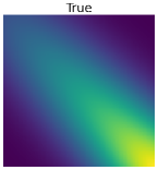
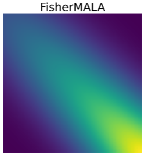
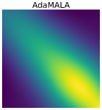
Figure 6: The covariance matrices for the GP target, where in the right panel is the covariance estimated by AdaMALA which was not displayed in Figure 1 in the main text.

We consider a Gaussian process to construct a 100-dimensional Gaussian where the covariance matrix is obtained by a non-stationary covariance function comprising the product of linear and squared exponential kernels plus small white noise, i.e. $[\Sigma]_{i,j}=s_{i}s_{j}\exp\{-\frac{1}{2}\frac{(s_{i}-s_{j})^{2}}{0.09}\}+0.001\delta_{i,j}$ where the scalar inputs $s_{i}$ form a regular grid in the range $[1,2]$. Figure 1b shows the evolution of the Frobenius norms and panels d,c depict as $100\times 100$ images the true covariance matrix and the preconditioner estimated by FisherMALA. For AdaMALA see Figure 6 in the Appendix. Clearly, FisherMALA learns much faster and achieves more accurate estimates of the optimal preconditioner. Further Table 1 shows that FisherMALA achieves significantly better ESS than AdaMALA and reaches the same performance with mMALA.

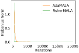
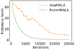
(a)	(b)	(c)	(d)

Figure 1: Panel (a) shows the Frobenius norm across burn-in iterations for the 2-D Gaussian and (b) for the GP target. The exact GP covariance matrix is shown in (c) and the estimated one by FisherMALA in (d).

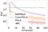
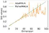
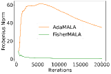
(a)	(b)	(c)

Figure 2: Results in the inhomogeneous Gaussian target.

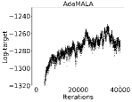
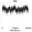
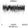
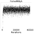
Figure 3: The evolution of the log-target across iterations for the best four algorithms in Caravan dataset.

Inhomogeneous Gaussian target.

In the last example we follow neal2010 ; rosenthal2011optimal and we consider a Gaussian target with diagonal covariance matrix $\Sigma=\text{diag}(\sigma^{2}_{1},\ldots,\sigma_{100}^{2})$ where the standard deviation values $\sigma_{i}$ take values in the grid $\{0.01,0.02,\dots,1\}$. This target is challenging because the different scaling across dimensions means that samplers with a single step size, i.e. without preconditioning, will adapt to the smallest dimension $x_{1}$ of the state while the chain at the higher dimensions, such as $x_{100}$, will be moving slowly exhibiting high autocorrelation. Note that FisherMALA and AdaMALA run without knowing that the optimal preconditioner is a diagonal matrix, i.e.  they learn a full covariance matrix. Figure 2a shows the ESS scores for all 100 dimensions of $x$ for four samplers (except mMALA which has the same performance with FisherMALA), where we can observe that only FisherMALA is able to achieve high ESS uniformly well across all dimensions. In contrast, MALA and HMC that use a single step size cannot achieve high sampling efficiency and their ESS for dimensions close to $x_{100}$ drops significantly. The same holds for AdaMALA due to its inability to learn fast the preconditioner, as shown by the Frobenius norm values in Figure 2c and the estimated standard deviations in Figure 2b. AdaMALA can eventually get very close to the optimal precondtioner but it requires hundred of thousands of adaptive steps, while FisherMALA learns it with only few thousand steps.

Table 1: ESS scores are averages after repeating the simulations $10$ times under different random initializations.

	Max ESS	Median ESS	Min ESS
GP target ($d=100$)
MALA	$15.235\pm 4.246$	$6.326\pm 1.934$	$3.619\pm 0.956$
AdaMALA	$845.100\pm 80.472$	$662.978\pm 81.127$	$552.377\pm 74.441$
HMC	$17.625\pm 6.706$	$6.680\pm 2.205$	$4.315\pm 0.889$
mMALA	$2109.441\pm 101.553$	$2007.640\pm 104.867$	$1841.978\pm 114.266$
FisherMALA	$2096.259\pm 94.751$	$1923.753\pm 95.820$	$1784.962\pm 104.440$
Pima Indian ($d=7$)
MALA	$106.668\pm 29.601$	$14.723\pm 3.821$	$4.061\pm 1.587$
AdaMALA	$211.948\pm 133.363$	$52.277\pm 26.566$	$6.401\pm 3.344$
HMC	$1624.773\pm 544.777$	$337.100\pm 212.158$	$6.052\pm 2.062$
mMALA	$6086.948\pm 117.241$	$5690.967\pm 118.401$	$5297.835\pm 160.084$
FisherMALA	$6437.419\pm 207.548$	$5981.960\pm 156.072$	$5628.541\pm 168.425$
Caravan ($d=87$)
MALA	$27.247\pm 7.554$	$5.890\pm 0.398$	$2.906\pm 0.150$
AdaMALA	$41.522\pm 9.343$	$7.144\pm 0.663$	$3.144\pm 0.135$
HMC	$787.901\pm 173.863$	$37.303\pm 6.808$	$4.238\pm 0.532$
mMALA	$179.899\pm 61.502$	$121.867\pm 41.801$	$51.414\pm 24.995$
FisherMALA	$2257.737\pm 45.289$	$1920.903\pm 55.821$	${\bf 498.016}\pm 96.692$
MNIST ($d=785$)
MALA	$34.074\pm 4.977$	$7.589\pm 0.149$	$2.944\pm 0.066$
AdaMALA	$62.301\pm 9.203$	$8.188\pm 0.399$	$2.985\pm 0.089$
HMC	$889.386\pm 118.050$	$303.345\pm 10.976$	$114.439\pm 20.965$
mMALA	$51.589\pm 3.447$	$20.222\pm 1.259$	$5.240\pm 0.492$
FisherMALA	$1053.455\pm 35.680$	$811.522\pm 19.165$	${\bf 439.580}\pm 52.800$

5.3 Bayesian logistic regression

We consider Bayesian logistic regression distributions of the form $\pi(\theta|Y,Z)\propto p(Y|\theta,Z)p(\theta)$ with data $(Y,Z)=\{y_{i},z_{i}\}_{i=1}^{m}$, where $z_{i}\in\mathbb{R}^{d}$ is the input vector and $y_{i}$ the binary label. The likelihood is $p(Y|\theta,Z)=\prod_{i=1}^{m}\sigma(\theta^{\top}z_{i})^{y_{i}}(1-\sigma(\theta^{\top}z_{i}))^{1-y_{i}}$, where $\theta\in\mathbb{R}^{d}$ are the random parameters assigned the prior $p(\theta)=\mathcal{N}(\theta|0,I_{d})$. We consider six binary classification datasets (Australian Credit, Heart, Pima Indian, Ripley, German Credit and Caravan) with a number of data ranging from $n=250$ to $n=5822$ and dimensionality of the $\theta$ ranging from $3$ to $87$. We also consider a much higher $785$-dimensional example on MNIST for classifying the digits $5$ and $6$, that has $11339$ training examples. To make the inference problems more challenging, in the first six examples we do not standardize the inputs $z_{i}$ which creates very anisotropic posteriors over $\theta$. For the MNIST data, which initially are grey-scale images in [0, 255], we simply divide by the maximum pixel value, i.e. 255, to bring the images in $[0,1]$. In Table 1 we report the ESS for the low $7$-dimensional Pima Indians dataset, the medium $87$-dimensional Caravan dataset and the higher $785$-dimensional MNIST dataset, while the results for the remaining datasets are shown in Appendix E. Further, Figure 3 shows the evolution of the unnormalized log target density $\log\{p(Y|\theta,Z)p(\theta)\}$ for the best four samplers in Caravan dataset which visualizes chain autocorrelation. From all these results we can conclude that FisherMALA is better than all other samplers, and remarkably it outperforms significantly the position-dependent mMALA, especially in the high dimensional Caravan and MNIST datasets.

6 Related Work

There exist works that use some form of global preconditioning in gradient-based samplers for specialized targets such as latent Gaussian models (Cotter2013mcmc, ; titsiasPapaspiliopoulos16, ), which make use of the tractable Gaussian prior. Our method differs, since it is more agnostic to the target and learns a preconditioning from the history of gradients, analogously to how traditional adaptive MCMC learns from states (haario2001adaptive, ; roberts2009examples, ).

Several research works use position-dependent preconditioning $A(x)$ within gradient-based samplers, such as MALA. This is for example the idea behind Riemannian manifold MALA (GirolamiCalderhead11, ) and extensions (Xifara14, ). Similar to Riemannian manifold methods there are approaches inspired by second order optimization that use the Hessian matrix, or some estimate of the Hessian, for sampling in a MALA-style manner (Qi_hessian-basedmarkov, ; gewekeTanizaki, ; stochasticNewtonmcmc, ). Recently, such samplers and their time-continuous diffusion limits have been theoretically analyzed by obtaining convergence guarantees (Chewietal2020, ; Li_mirrorLangevin2022, ). All such methods form a position-dependent preconditioning and not the preconditioning we use in this paper, e.g. note that $\mathcal{I}^{-1}$ we consider here requires an expectation under the target and thus it is always a global preconditioner rather than a position-dependent one. Another difference is that our method has quadratic cost, while position-dependent preconditioning methods have cubic cost and they require computationally demanding quantities like the Hessian matrix. Therefore, in order for these methods to run faster some approximation may be needed, e.g. low rank (stochasticNewtonmcmc, ) or quasi-Newton type (ZhangS11, ; ensemblepreconditioning, ). Furthermore, the Bayesian logistic results in Table 1 (see also Figure 3) show that the proposed FisherMALA method significantly outperforms manifold MALA (GirolamiCalderhead11, ) in Caravan and MNIST examples, despite the fact that manifold MALA preconditions with the exact negative inverse Hessian matrix of the log target. This could suggest that position-dependent preconditioning may be less effective in certain type of high-dimensional and log-concave problems.

Finally, there is recent work for learning flexible MCMC proposals by using neural networks (song2017nice, ; levy2018generalizing, ; habib2018auxiliary, ; Salimans2015, ) and by adapting parameters using differentiable objectives (levy2018generalizing, ; neklyudov2018metropolis, ; TitsiasDellaportas19, ; Dharamshietal23, ). Our method differs, since it does not use objective functions (which have extra cost because they require an optimization to run in parallel with the MCMC chain), but instead it adapts similarly to traditionally MCMC methods by accumulating information from the observed history of the chain.

7 Conclusion

We derived an optimal preconditioning for the Langevin diffusion by optimizing the expected squared jumped distance, and subsequently we developed an adaptive MCMC algorithm that approximates the optimal preconditioning by applying an efficient quadratic cost recursion. Some possible topics for future research are: Firstly, it would be useful to investigate whether the score function differences that we use as the adaptation signal introduce any bias in the estimation of the inverse Fisher matrix. Secondly, it would be interesting to extend our method to learn the preconditioning for other gradient-based samplers such as Hamiltonian Monte Carlo (HMC), where such a matrix there is referred to as the inverse mass matrix. For HMC this is more complex since both the mass matrix and its inverse are needed in the iteration. Finally, it could be interesting to investigate adaptive schemes of the inverse Fisher matrix by using multiple parallel and interacting chains, similarly to ensemble covariance matrix estimation for Langevin diffusions Garbuno2020 .

Appendix A Proofs

A.1 Proof of Proposition 1

The difference between the logarithm of the backward and forward proposals of preconditioned MALA, i.e. the quantity $\log q(x_{n}|y_{n})-\log q(y_{n}|x_{n})$ can be written (ignoring the normalizing constants of the Gaussians which trivially cancel out) as,

$$-\frac{1}{2\sigma^{2}}\left(x_{n}-y_{n}-\frac{\sigma^{2}}{2}A\nabla\log\pi(y_{n})\right)^{\top}A^{-1}\left(x_{n}-y_{n}-\frac{\sigma^{2}}{2}A\nabla\log\pi(y_{n})\right)$$

$$+\frac{1}{2\sigma^{2}}\left(y_{n}-x_{n}-\frac{\sigma^{2}}{2}A\nabla\log\pi(x_{n})\right)^{\top}A^{-1}\left(y_{n}-x_{n}-\frac{\sigma^{2}}{2}A\nabla\log\pi(x_{n})\right).$$ (18)

Observe that the term $\frac{1}{2\sigma^{2}}(x_{n}-y_{n})^{\top}A^{-1}(x_{n}-y_{n})$ cancels out since it appears twice with opposite sign. The remaining terms after some simple algebra simplify as

$${\color[rgb]{0,0,1}\frac{1}{2}\!\left(x_{n}-y_{n}-\frac{\sigma^{2}}{4}A\nabla\log\pi(y_{n})\right)^{\top}\!\!\nabla\log\pi(y_{n})}-{\color[rgb]{1,0,0}\frac{1}{2}\!\left(y_{n}-x_{n}-\frac{\sigma^{2}}{4}A\nabla\log\pi(x_{n})\right)^{\top}\!\!\nabla\log\pi(x_{n})}$$

$$={\color[rgb]{0,0,1}h(x_{n},y_{n})}-{\color[rgb]{1,0,0}h(y_{n},x_{n})}$$ (19)

which completes the proof.

A.2 Proof of Proposition 2

We assume $x_{t}\sim\pi(x_{t})$. Then by taking the expectation of the r.h.s. of Eq. (4) (where the expectation is taken w.r.t. $x_{t}$ and the independent Brownian motion increment $B_{t+\delta}-B_{t}\sim\mathcal{N}(0,\delta I_{d})$) and noting that $\mathbb{E}_{\pi(x_{t})}[\nabla\log\pi(x_{t})]=0$ and $\mathbb{E}[B_{t+\delta}-B_{t}]=0$ we conclude that $\mathbb{E}[x_{t+\delta}-x_{t}]=0$. Then the covariance is

$$\mathbb{E}[(x_{t+\delta}-x_{t})(x_{t+\delta}-x_{t})^{\top}]=$$

$$=\mathbb{E}\left[(\frac{\delta}{2}A\nabla\log\pi(x_{t})+\sqrt{A}(B_{t+\delta}-B_{t}))(\frac{\delta}{2}A\nabla\log\pi(x_{t})+\sqrt{A}(B_{t+\delta}-B_{t}))^{\top}\right]$$

$$=\frac{\delta^{2}}{4}A\mathbb{E}_{\pi(x_{t})}[\nabla\log\pi(x_{t})\nabla\log\pi(x_{t})^{\top}]A+\delta A$$

$$=\frac{\delta^{2}}{4}A\mathcal{I}A+\delta A,$$

where we used that $\mathbb{E}[(B_{t+\delta}-B_{t})(B_{t+\delta}-B_{t})^{\top}]=\delta I_{d}$ , $\sqrt{A}\sqrt{A}^{\top}=A$ and that the cross covariance terms are zero.

A.3 Proof of Proposition 3

The expected squared jumped distance is written as

$$J(\delta,A)=\text{tr}\left(\frac{\delta^{2}}{4}A\mathcal{I}A+\delta A\right)=\frac{\delta^{2}}{4}\text{tr}(A\mathcal{I}A)+\delta c,$$

where we used the constraint $\text{tr}(A)=c$. Since $c$ is just a constant to minimize $J(\delta,A)$ is the same as minimizing $\text{tr}(A\mathcal{I}A)$, a quadratic convex loss since $\mathcal{I}$ is positive definite, under the constraint that $A$ is symmetric positive definite matrix and $\text{tr}(A)=c$. To deal with the equality constraint we consider the Lagrangian

$$\text{tr}(A\mathcal{I}A)-\lambda(\text{tr}(A)-c).$$

By taking derivatives wrt the matrix $A$ (using the matrix derivative identities $\frac{\partial}{\partial X}\text{tr}(XBX)=X^{\top}B^{\top}+B^{\top}X^{\top}$ and $\frac{\partial}{\partial X}\text{tr}(X)=I_{d}$ for arbitrary $d\times d$ square matrices $X,B$) and setting to zero we see that $A$ must satisfy the linear equation

$$A^{\top}\mathcal{I}+\mathcal{I}A^{\top}=\lambda I_{d},$$

where we used that $\mathcal{I}$ is a symmetric matrix. This is a set of linear equations and given that each eigenvalue $\mu_{i}$ of $\mathcal{I}$ satisfies $0<\mu_{i}<\infty$, so that $\mathcal{I}$ is invertible, there is an unique solution given by $A=(1/2)\lambda\mathcal{I}^{-1}$. The Lagrange multiplier $\lambda$ is chosen so that $\text{tr}(A)=c$ which leads to the optimal $A^{*}$

$$A^{*}=\frac{c}{\sum_{i=1}^{d}\frac{1}{\mu_{i}}}\mathcal{I}^{-1}.$$

Note that $A^{*}$ turned out to be symmetric and positive definite as desired. For this $A^{*}$ the optimal loss value is $\text{tr}(A^{*}\mathcal{I}A^{*})=\frac{c^{2}}{\sum_{i=1}\frac{1}{\mu_{i}}}$, for which we further need to disambiguate whether this is the global minimum or maximum. We can do this by choosing a different matrix that satisfies the constraint $\text{tr}(A)=c$ and compare its loss with the optimal loss $\frac{c^{2}}{\sum_{i=1}^{d}\frac{1}{\mu_{i}}}$ . For example, one such matrix is $A=\frac{c}{d}I_{d}$, which has loss value $\frac{c^{2}(\sum_{i=1}^{d}\mu_{i})}{d^{2}}$. Then by using the Cauchy-Schwarz inequality $d^{2}=(\sum_{i=1}^{d}\frac{\sqrt{\mu_{i}}}{\sqrt{\mu_{i}}})^{2}\leq(\sum_{i=1}^{d}\mu_{i})(\sum_{i=1}^{d}\frac{1}{\mu}_{i})$ we obtain $\frac{c^{2}(\sum_{i=1}^{d}\mu_{i})}{d^{2}}\geq\frac{c^{2}(\sum_{i=1}^{d}\mu_{i})}{(\sum_{i=1}^{d}\mu_{i})(\sum_{i=1}^{d}\frac{1}{\mu}_{i})}=\frac{c^{2}}{\sum_{i=1}\frac{1}{\mu_{i}}}$. This shows that $A^{*}$ achieves the global minimum which completes the proof.

A.4 Proof of Proposition 4

We first state and prove the following intermediate result.

Lemma 1.

Suppose the positive definite matrix $I_{d}-zz^{\top}$ where $z\in\mathbb{R}^{d}$ and $z^{\top}z\leq 1$. Then, a square root matrix $R$, satisfying $RR^{\top}=A$, has the form $R=I_{d}-rzz^{\top}$ where $r=\frac{1}{1+\sqrt{1-z^{\top}z}}$.

Proof.

We hypothesize that $R$ has the form $I_{d}-rzz^{\top}$ for some scalar $r$. Then since $RR^{\top}=I_{d}-zz^{\top}$ we see that $r$ must satisfy the quadratic equation $r^{2}z^{\top}z-2r+1=0$, which has two real solutions $\frac{1\pm\sqrt{1-z^{\top}z}}{z^{\top}z}$ and we will use $\frac{1-\sqrt{1-z^{\top}z}}{z^{\top}z}\leq 1$ which ensures $R$ is positive definite. This solution can also be written as $r=\frac{1}{1+\sqrt{1-z^{\top}z}}$. ∎

To prove the proposition we need to find a square root matrix $R_{1}$ of $A_{1}=\frac{1}{\lambda}\left(I_{d}-\frac{s_{1}s_{1}^{\top}}{\lambda+s_{1}^{\top}s_{1}}\right)$ where we clearly need to specify a square root matrix for $I_{d}-\frac{s_{1}s_{1}^{\top}}{\lambda+s_{1}^{\top}s_{1}}$. We observe that by setting $z=\frac{s_{1}}{\sqrt{\lambda+s_{1}^{\top}s_{1}}}$ Lemma 1 is applicable so that the square root matrix is

$$R_{1}=\frac{1}{\sqrt{\lambda}}\left(I_{d}-r_{1}\frac{s_{1}s_{1}^{\top}}{\lambda+s_{1}^{\top}s_{1}}\right),\ \ r_{1}=\frac{1}{1+\sqrt{\frac{\lambda}{\lambda+s_{1}^{\top}s_{1}}}}.$$

Similarly by applying again Lemma 1 we can find $R_{n}$ for any $n>1$.

The computation of $R_{n}$ costs $O(d^{2})$ per iteration. Firstly, the vector $\phi_{n}=R_{n-1}^{\top}s_{n}$ is computed which is a matrix-vector multiplication. The next step is to compute the scalar $r_{n}$ in $O(d)$ (involving the dot product $\phi_{n}^{\top}\phi_{n}$) and then the scaled vector $\phi_{n}^{\prime}=\frac{r_{n}}{1+\phi_{n}^{\top}\phi_{n}}\phi_{n}$ also an $O(d)$ operation. Then we need two additional $O(d^{2})$ multiplication operations to obtain firstly the vector $t_{n}=R_{n-1}\phi_{n}$ and secondly the outer vector product $t_{n}(\phi_{n}^{\prime})^{\top}$. Finally, the update is $R_{n}=R_{n-1}-t_{n}(\phi_{n}^{\prime})^{\top}$ which requires a final $O(d^{2})$ addition operation of two matrices which is typically cheaper than $O(d^{2})$ multiplication. Therefore, overall the cost is $O(d^{2})$.

Appendix B Generalizing the recursion over arbitrary learning rate sequences

Suppose we have a sequence of learning rates $\gamma_{1},\gamma_{2},\ldots,$. Then a stochastic approximation of the Fisher matrix $\mathcal{I}$ takes the form

$$\mathcal{I}_{n}=\mathcal{I}_{n-1}+\gamma_{n}(s_{n}s_{n}^{\top}-\mathcal{I}_{n-1})=(1-\gamma_{n})\mathcal{I}_{n-1}+\gamma_{n}s_{n}s_{n}^{\top},$$

where the sequence is initialized at $\mathcal{I}_{1}=s_{1}s_{1}^{\top}+\lambda I$. The inverse of the empirical Fisher is written as

$$A_{n}=\left((1-\gamma_{n})\mathcal{I}_{n-1}+\gamma_{n}s_{n}s_{n}^{\top}\right)^{-1}=\frac{1}{1-\gamma_{n}}\left(A_{n-1}-\frac{A_{n-1}s_{n}s_{n}^{\top}A_{n-1}}{\frac{1-\gamma_{n}}{\gamma_{n}}+s_{n}^{\top}\mathcal{I}_{n-1}^{-1}s_{n}}\right),$$

which is initialized at $A_{1}=\frac{1}{\lambda}\left(I_{d}-\frac{s_{1}s_{1}^{\top}}{\lambda+s_{1}^{\top}s_{1}}\right)$ for which the square root $R_{1}$ is the same as for the standard learning rate $\gamma_{n}=1/n$. The square root recursion for $n>1$ takes the form

$$R_{n}=\frac{1}{\sqrt{1-\gamma_{n}}}\left(R_{n-1}-r_{n}\frac{(R_{n-1}\phi_{n})\phi_{n}^{\top}}{(1-\gamma_{n})/\gamma_{n}+\phi_{n}^{\top}\phi_{n}}\right),\ \phi_{n}=R_{n}^{\top}s_{n},\ r_{n}=\frac{1}{1+\sqrt{\frac{(1-\gamma_{n})/\gamma_{n}}{(1-\gamma_{n})/\gamma_{n}+\phi_{n}^{\top}\phi_{n}}}}.$$

Appendix C FisherMALA with paired mean and covariance stochastic approximation

Here, we derive a recursion for the empirical Fisher that centers the score function vectors using the standard procedure by recursively estimating also the mean. We start from the following consistent estimator of the inverse Fisher:

$$A_{n}=\left(\frac{1}{n-1}\sum_{i=1}^{n}(s_{i}-\bar{s}_{n})(s_{i}-\bar{s}_{n})^{\top}+\frac{\lambda}{n-1}I_{d}\right)^{-1},$$

where $\bar{s}_{n}=\frac{1}{n}\sum_{i=1}^{n}s_{i}$. This follows the recursion

$$A_{n} =\left(\frac{n-2}{n-1}A_{n-1}^{-1}+\frac{1}{n}\delta_{n}\delta_{n}^{\top}\right)^{-1}=\frac{n-1}{n-2}A_{n-1}-\frac{(n-1)^{2}}{(n-2)^{2}}\frac{A_{n-1}\delta_{n}\delta_{n}^{\top}A_{n-1}}{n+\frac{n-1}{n-2}\delta_{n}^{\top}A_{n-1}\delta_{n}}$$

$$=\frac{1}{\lambda_{n-1}}\left(A_{n-1}-\frac{A_{n-1}\delta_{n}\delta_{n}^{\top}A_{n-1}}{n\lambda_{n-1}+\delta_{n}^{\top}A_{n-1}\delta_{n}}\right).$$

Here, $\delta_{n}=s_{n}-\bar{s}_{n-1}$ and we defined the sequence of scalars $\lambda_{n}=\frac{n-1}{n}$, for $n\geq 2$ while the starting point of this sequence $n=1$ we define it to be equal to the parameter parameter $\lambda$, i.e. $\lambda_{1}=\lambda>0$. The recursion starts at $A_{2}$ given by

$$A_{2}=\left(\frac{1}{2}\delta_{2}\delta_{2}^{\top}+\lambda_{1}I\right)^{-1}=\frac{1}{\lambda_{1}}\left(I_{d}-\frac{\delta_{2}\delta_{2}^{\top}}{2\lambda_{1}+\delta_{2}^{\top}\delta_{2}}\right),$$

where $\delta_{2}=s_{2}-s_{1}$. Along with the above we recursively estimate also the mean vector (for $n\geq 1$): $\bar{s}_{n}=\frac{n-1}{n}\bar{s}_{n-1}+\frac{1}{n}s_{n}$.

To express a recursion of square root matrix, such that $A_{n}=R_{n}R_{n}^{\top}$ we first write

$$A_{n} =\frac{1}{\lambda_{n-1}}R_{n-1}\left(I_{d}-\frac{R_{n-1}^{\top}\delta_{n}\delta_{n}^{\top}R_{n-1}}{n\lambda_{n-1}+\delta_{n}^{\top}A_{n-1}\delta_{n}}\right)R_{n-1}^{\top}$$

$$=\frac{1}{\lambda_{n-1}}R_{n-1}\left(I_{d}-\frac{\phi_{n}\phi_{n}^{\top}}{n\lambda_{n-1}+\phi_{n}^{\top}\phi_{n}}\right)R_{n-1}^{\top}.$$

Then we can recognize the square root recursion as

$$R_{n}=\frac{1}{\sqrt{\lambda_{n-1}}}R_{n-1}\left(I_{d}-r_{n}\frac{\phi_{n}\phi_{n}^{\top}}{n\lambda_{n-1}+\phi_{n}^{\top}\phi_{n}}\right),\ \ r_{n}=\frac{1}{1+\sqrt{\frac{n\lambda_{n-1}}{n\lambda_{n-1}+\phi_{n}^{\top}\phi_{n}}}},$$

which is initialized at $R_{2}=\frac{1}{\sqrt{\lambda_{1}}}\left(I_{d}-r_{2}\frac{\delta_{2}\delta_{2}^{\top}}{2\lambda_{1}+\delta_{2}^{\top}\delta_{2}}\right),\ \ r_{2}=\frac{1}{1+\sqrt{\frac{2\lambda_{1}}{2\lambda_{1}+\delta_{2}^{\top}\delta_{2}}}}.$

Appendix D Initialization of AdaMALA

To initialize AdaMALA we first perform $n_{0}=500$ iterations with simple MALA where we adapt the step size parameter $\sigma^{2}$. Thus, this part of the initialization is exactly the same used by FisherMALA. However, for AdaMALA we do an additional set of $n_{0}=500$ iterations where simple MALA still runs and collects samples which are used to sequentially update the empirical covariance matrix $\Sigma_{n}$. The purpose of this second phase is to play the role of "warm-up" and provide a reasonable initialization for $\Sigma_{n}$. After the second phase (so in total $1000$ iterations) AdaMALA starts running having as a preconditioner $\Sigma_{n}$, which keeps adapted in every iteration until the last burn-in iteration.

Appendix E Additional results

E.1 The step size $\sigma^{2}$ is maximized when preconditioning becomes effective

To experimentally backup our claims in Section 3 that the discretization step size, denoted there by $\delta$ or $\sigma^{2}$, gets large when the preconditioner is selected efficiently, in Figure 4 we report the final learned values (after burn-in adaptation iterations) of $\sigma^{2}$ for MALA, AdaMALA and FisherMALA. For all these three algorithms the values of $\sigma^{2}$ are comparable because all use an overall preconditioning of the form $\frac{\sigma^{2}}{\frac{1}{d}\text{tr}(A)}A$ and only the matrix $A$ is changing among them. For example, simple MALA sets this matrix to $A=I_{d}$, while AdaMALA and FisherMALA use their own procedures to learn more complex matrices. Figure 4 shows the estimated $\sigma^{2}$, for the four datasets reported in the main text in Table 1. This shows that FisherMALA achieves significantly larger $\sigma^{2}$ in all cases, which can be orders of magnitude larger than the two other algorithms (note the $y$ axis in Figure 4 is in log scale).

GP target	Pima Indian
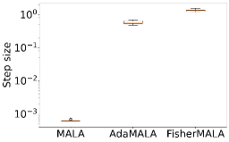
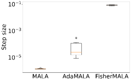
Caravan	MNIST

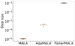
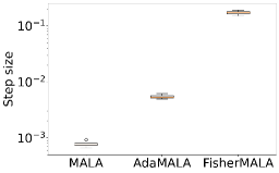
Figure 4: It shows the estimated values of $\sigma^{2}$ for MALA, AdaMALA and FisherMALA using boxplots (each computed from the 10 random repeats; see Table 1) for the four datasets presented in Table 1. For better visibility the $y$ axis is shown in log scale.

E.2 Additional plots and tables

Figure 5 and 6 display additional visualizations for the 2-D Gaussian and the GP target experiments. Tables 2-6 provide the ESS scores for the inhomogeneous Gaussian target and all remaining Bayesian logistic regression datasets, that were not included in the main paper. Bold font in the "Min ESS" entry in the tables indicates statistical significance. Similarly, Figures 7-14 show the log target values across iterations for the four best samplers, i.e. excluding simple MALA which is the least performing method.

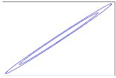
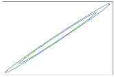
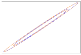
(a)	(b)	(c)

Figure 5: Panel (a) shows the true covariance of the 2-D Gaussian. Panel (b) shows the estimated covariance by FisherMALA (dashed green line), where for comparison the true covariance is also shown in blue. Panel (c) shows the estimated covariance by AdaMALA (dashed red line).

Table 2: ESS scores for the inhomogeneous Gaussian target.

	Max ESS	Median ESS	Min ESS
MALA	$13695.291\pm 1369.515$	$9.793\pm 0.655$	$2.943\pm 0.130$
AdaMALA	$4310.690\pm 606.618$	$70.802\pm 14.912$	$9.225\pm 3.272$
HMC	$19362.103\pm 1372.400$	$381.205\pm 101.781$	$42.033\pm 33.080$
mMALA	$2354.354\pm 65.835$	$2014.801\pm 23.713$	$1490.119\pm 108.745$
FisherMALA	$2347.340\pm 70.234$	$2002.579\pm 30.001$	$1500.983\pm 67.087$

Table 3: ESS scores for the Heart dataset.

	Max ESS	Median ESS	Min ESS
MALA	$68.774\pm 25.304$	$5.354\pm 1.056$	$2.898\pm 0.104$
AdaMALA	$208.636\pm 124.762$	$14.762\pm 9.134$	$3.781\pm 0.731$
HMC	$387.321\pm 311.673$	$12.991\pm 4.009$	$4.064\pm 1.120$
mMALA	$878.858\pm 1079.674$	$789.356\pm 969.806$	$651.793\pm 806.477$
FisherMALA	$4864.278\pm 103.277$	$4474.288\pm 102.029$	${\bf 3954.793}\pm 199.832$

Table 4: ESS scores for the German Credit dataset.

	Max ESS	Median ESS	Min ESS
MALA	$262.206\pm 211.839$	$5.932\pm 0.668$	$2.972\pm 0.212$
AdaMALA	$223.592\pm 111.914$	$16.111\pm 5.058$	$3.774\pm 0.653$
HMC	$10439.824\pm 9572.157$	$45.872\pm 7.823$	$5.431\pm 1.257$
mMALA	$3066.605\pm 100.768$	$2767.022\pm 94.222$	$2342.902\pm 112.610$
FisherMALA	$3951.807\pm 78.858$	$3582.184\pm 90.551$	${\bf 3011.483}\pm 258.154$

Table 5: ESS scores for the Australian Credit dataset.

	Max ESS	Median ESS	Min ESS
MALA	$15.627\pm 12.892$	$3.823\pm 1.166$	$2.611\pm 0.538$
AdaMALA	$1525.373\pm 1600.986$	$6.986\pm 3.200$	$3.297\pm 0.456$
HMC	$1282.235\pm 932.038$	$6.966\pm 1.249$	$2.856\pm 0.095$
mMALA	$2609.462\pm 881.967$	$2308.175\pm 776.872$	$1869.364\pm 630.880$
FisherMALA	$4732.724\pm 116.074$	$4361.969\pm 104.750$	${\bf 3772.086}\pm 265.170$

Table 6: ESS scores for the Ripley dataset.

	Max ESS	Median ESS	Min ESS
MALA	$2058.325\pm 180.839$	$496.981\pm 68.029$	$427.492\pm 60.006$
AdaMALA	$9678.793\pm 384.295$	$9497.814\pm 463.059$	$9272.026\pm 412.361$
HMC	$18403.796\pm 3202.136$	$18254.161\pm 3513.550$	$7644.709\pm 2288.559$
mMALA	$9333.633\pm 280.238$	$8941.579\pm 288.223$	$8655.640\pm 396.106$
FisherMALA	$9875.968\pm 218.801$	$9673.009\pm 280.759$	$9244.631\pm 559.137$

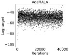
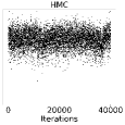
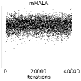
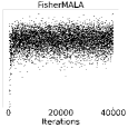
Figure 7: The evolution of the log-target across iterations in the GP target.

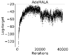
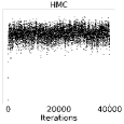
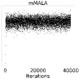
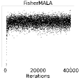
Figure 8: The evolution of the log-target across iterations in the inhomogeneous Gaussian target.

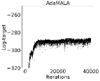
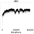
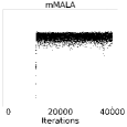
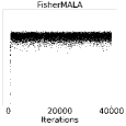
Figure 9: The evolution of the log-target across iterations in Pima Indians dataset.

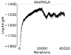
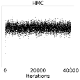
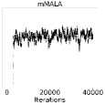
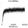
Figure 10: The evolution of the log-target across iterations in MNIST dataset.

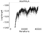
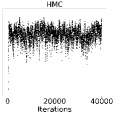
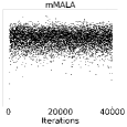
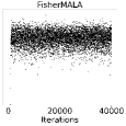
Figure 11: The evolution of the log-target across iterations in German Credit dataset.

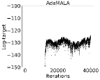
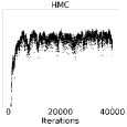
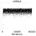
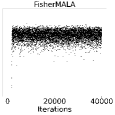
Figure 12: The evolution of the log-target across iterations in Heart dataset.

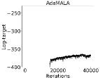
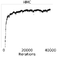
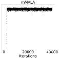
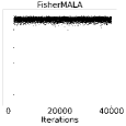
Figure 13: The evolution of the log-target across iterations in Australian Credit dataset.

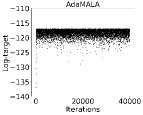
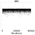
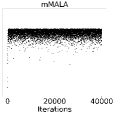
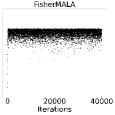
Figure 14: The evolution of the log-target across iterations in Ripley dataset.

E.3 The effect of Raoblackwellization and comparison with paired stochastic estimation

Finally, we compare three versions of FisherMALA: (i) The one that uses the Raoblackwellized signal $s_{n}^{\delta}$ from Eq. (16), which is our main proposed method used in the main paper and all previous results (in this section we will denote this as FisherMALA-with-RB), (ii) the one that uses the initial score function difference from Eq. (15) (FisherMALA-no-RB) and (iii) and FisherMALA with paired mean and covariance stochastic estimation (FisherMALA-paired-est) as descibed in Appendix C. Table 7 compares the three versions of FisherMALA in terms of ESS for all problems, which shows that FisherMALA-paired-est is significantly worse than the other two methods that learn based on score function increments. These two latter methods, FisherMALA-with-RB and FisherMALA-no-RB, have similar performance without significant difference (the highest difference in terms of Min ESS is in Pima Indians dataset, but still not statistically significant).

Figure 15 displays the Frobenius norms for FisherMALA with Raoblackwellization and FisherMALA without Raoblackwellization in the two $100$-dimensional Gaussian targets. It shows that the Raoblackwellized signal $s_{n}^{\delta}$ leads to slightly faster convergence, which agrees with the theory that says that Raoblackwellization should reduce the variance.

Finally, Table 8 reports numerical performance of the non-centered version of FisherMALA where we learn directly from the score function vectors $s_{n}$, i.e. without centering or using score function increments. From this table we can see that FisherMALA (non-centered) performs worse than the other FisherMALA variants, and only on Ripley dataset works equally well with the rest.

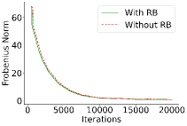
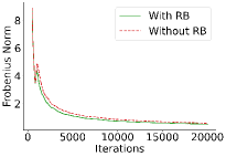
Figure 15: The effect of Raoblackwellization. Left panel shows the evolution of the Frobenius norm in the GP target and right panel for the inhomogeneous Gaussian target.

Table 7: Comparison of ESS scores for three versions of FisherMALA: the first with Raoblackwellized score function differences in (16), the second based on the initial adaptation signal of score function differences from (15), and the third based on paired stochastic estimation.

	Max ESS	Median ESS	Min ESS
GP target
FisherMALA-with-RB	$2096.259\pm 94.751$	$1923.753\pm 95.820$	$1784.962\pm 104.440$
FisherMALA-no-RB	$2064.940\pm 87.943$	$1916.990\pm 85.208$	$1794.114\pm 103.711$
FisherMALA-paired-est	$1802.141\pm 142.784$	$1583.570\pm 109.241$	$1226.303\pm 244.752$
Inhomog. Gaussian
FisherMALA-with-RB	$2347.340\pm 70.234$	$2002.579\pm 30.001$	$1500.983\pm 67.087$
FisherMALA-no-RB	$2351.481\pm 78.894$	$2012.243\pm 30.024$	$1489.617\pm 133.619$
FisherMALA-paired-est	$1941.994\pm 106.710$	$1147.138\pm 61.591$	$109.160\pm 57.998$
Heart
FisherMALA-with-RB	$4864.278\pm 103.277$	$4474.288\pm 102.029$	$3954.793\pm 199.832$
FisherMALA-no-RB	$4893.063\pm 107.068$	$4455.591\pm 98.542$	$3977.741\pm 194.922$
FisherMALA-paired-est	$4804.365\pm 176.747$	$2519.187\pm 693.945$	$441.434\pm 386.287$
German Credit
FisherMALA-with-RB	$3951.807\pm 78.858$	$3582.184\pm 90.551$	$3011.483\pm 258.154$
FisherMALA-no-RB	$3979.744\pm 79.647$	$3616.894\pm 104.722$	$3031.384\pm 228.345$
FisherMALA-paired-est	$3960.773\pm 105.169$	$3097.557\pm 252.619$	$397.034\pm 244.768$
Australian Credit
FisherMALA-with-RB	$4732.724\pm 116.074$	$4361.969\pm 104.750$	$3772.086\pm 265.170$
FisherMALA-no-RB	$4711.549\pm 115.329$	$4364.347\pm 95.004$	$3790.949\pm 253.464$
FisherMALA-paired-est	$4887.606\pm 173.626$	$3603.765\pm 725.018$	$84.202\pm 44.750$
Ripley
FisherMALA-with-RB	$9875.968\pm 218.801$	$9673.009\pm 280.759$	$9244.631\pm 559.137$
FisherMALA-no-RB	$9852.895\pm 281.295$	$9679.384\pm 303.946$	$9272.040\pm 581.732$
FisherMALA-paired-est	$9869.053\pm 321.031$	$9598.430\pm 330.766$	$9217.330\pm 584.224$
Pima Indians
FisherMALA-with-RB	$6437.419\pm 207.548$	$5981.960\pm 156.072$	$5628.541\pm 168.425$
FisherMALA-no-RB	$6448.999\pm 199.817$	$5977.292\pm 122.852$	$5585.217\pm 160.586$
FisherMALA-paired-est	$6048.419\pm 650.262$	$2618.271\pm 889.425$	$788.687\pm 388.978$
Caravan
FisherMALA-with-RB	$2257.737\pm 45.289$	$1920.903\pm 55.821$	$498.016\pm 96.692$
FisherMALA-no-RB	$2241.262\pm 47.873$	$1908.045\pm 62.430$	$509.913\pm 115.563$
FisherMALA-paired-est	$1930.109\pm 208.848$	$1107.987\pm 83.439$	$87.456\pm 90.858$
MNIST
FisherMALA-with-RB	$1053.455\pm 35.680$	$811.522\pm 19.165$	$439.580\pm 52.800$
FisherMALA-no-RB	$1036.138\pm 32.399$	$803.210\pm 16.163$	$437.325\pm 40.040$
FisherMALA-paired est	$301.055\pm 37.597$	$13.819\pm 1.127$	$3.176\pm 0.113$

Table 8: Performance of FisherMALA (non-centered), in a subset of the targets, which learns directly from the score function vectors $s_{n}$.

	Max ESS	Median ESS	Min ESS
GP target
FisherMALA (non-centered)	$1740.943\pm 157.871$	$518.924\pm 579.639$	$48.218\pm 117.349$
Ripley
FisherMALA (non-centered)	$9881.540\pm 353.377$	$9636.357\pm 313.009$	$9237.885\pm 710.741$
Pima Indians
FisherMALA (non-centered)	$5520.181\pm 1781.518$	$474.990\pm 587.788$	$65.313\pm 59.316$
Caravan
FisherMALA (non-centered)	$1602.723\pm 164.497$	$14.226\pm 4.429$	$3.298\pm 0.141$
MNIST
FisherMALA (non-centered)	$271.629\pm 22.918$	$22.147\pm 1.683$	$3.744\pm 0.139$

References

• [1] Christophe Andrieu and Yves Atchade. On the efficiency of adaptive mcmc algorithms. Electronic Communications in Probability, 12:336–349, 2007.
• [2] Christophe Andrieu and Γ‰ric Moulines. On the ergodicity properties of some adaptive mcmc algorithms. The Annals of Applied Probability, 16(3):1462–1505, 2006.
• [3] Christophe Andrieu and Johannes Thoms. A tutorial on adaptive mcmc. Statistics and computing, 18(4):343–373, 2008.
• [4] Yves Atchade, Gersende Fort, Eric Moulines, and Pierre Priouret. Adaptive markov chain monte carlo: theory and methods. Preprint, 2009.
• [5] YvesΒ F AtchadΓ© and JeffreyΒ S Rosenthal. On adaptive markov chain monte carlo algorithms. Bernoulli, 11(5):815–828, 2005.
• [6] MylΓ¨ne BΓ©dard. Weak convergence of metropolis algorithms for non-iid target distributions. The Annals of Applied Probability, pages 1222–1244, 2007.
• [7] MylΓ¨ne BΓ©dard. Efficient sampling using metropolis algorithms: Applications of optimal scaling results. Journal of Computational and Graphical Statistics, 17(2):312–332, 2008.
• [8] Mylene Bedard. Optimal acceptance rates for metropolis algorithms: Moving beyond 0.234. Stochastic Processes and their Applications, 118(12):2198–2222, 2008.
• [9] Alexandros Beskos, Natesh Pillai, Gareth Roberts, Jesus-Maria Sanz-Serna, and Andrew Stuart. Optimal tuning of the hybrid monte carlo algorithm. Bernoulli, 19(5A):1501–1534, 2013.
• [10] GeraldΒ J. Bierman. Factorization Methods for Discrete Sequential Estimation, volume 128. 1977.
• [11] Steve Brooks, Andrew Gelman, Galin Jones, and Xiao-Li Meng. Handbook of Markov Chain Monte Carlo. CRC press, 2011.
• [12] Sinho Chewi, Thibaut LeΒ Gouic, Chen Lu, Tyler Maunu, Philippe Rigollet, and Austin Stromme. Exponential ergodicity of mirror-langevin diffusions. In Proceedings of the 34th International Conference on Neural Information Processing Systems, 2020.
• [13] S.Β L. Cotter, G.Β O. Roberts, A.Β M. Stuart, and D.Β White. MCMC methods for functions: modifying old algorithms to make them faster. Statistical Science, 28(3):424–446, 2013.
• [14] Ameer Dharamshi, Vivian Ngo, and JeffreyΒ S. Rosenthal. Sampling by divergence minimization. Communications in Statistics - Simulation and Computation, 2023.
• [15] Simon Duane, A.Β D. Kennedy, BrianΒ J. Pendleton, and Duncan Roweth. Hybrid monte carlo. Physics Letters B, 195(2):216 – 222, 1987.
• [16] Alfredo Garbuno-Inigo, Franca Hoffmann, Wuchen Li, and AndrewΒ M. Stuart. Interacting langevin diffusions: Gradient structure and ensemble kalman sampler. SIAM Journal on Applied Dynamical Systems, 19(1):412–441, 2020.
• [17] John Geweke and Hisashi Tanizaki. Note on the sampling distribution for the metropolis-hastings algorithm. Communications in Statistics - Theory and Methods, 32(4):775–789, 2003.
• [18] W.R. Gilks, S.Β Richardson, and D.Β Spiegelhalter. Markov Chain Monte Carlo in Practice. Chapman & Hall/CRC Interdisciplinary Statistics. Taylor & Francis, 1995.
• [19] Paolo Giordani and Robert Kohn. Adaptive independent metropolis–hastings by fast estimation of mixtures of normals. Journal of Computational and Graphical Statistics, 19(2):243–259, 2010.
• [20] Mark Girolami and Ben Calderhead. Riemann manifold Langevin and Hamiltonian Monte Carlo methods. Journal of the Royal Statistical Society: Series B (Statistical Methodology), 73(2):123–214, 2011.
• [21] Heikki Haario, Eero Saksman, and Johanna Tamminen. An adaptive metropolis algorithm. Bernoulli, 7(2):223–242, 2001.
• [22] Heikki Haario, Eero Saksman, and Johanna Tamminen. Componentwise adaptation for high dimensional mcmc. Computational Statistics, 20(2):265–273, 2005.
• [23] Raza Habib and David Barber. Auxiliary variational mcmc. To appear at ICLR 2019, 2019.
• [24] Benedict Leimkuhler, Charles Matthews, and Jonathan Weare. Ensemble preconditioning for markov chain monte carlo simulation. Statistics and Computing, 28, 03 2018.
• [25] Daniel Levy, MattΒ D. Hoffman, and Jascha Sohl-Dickstein. Generalizing hamiltonian monte carlo with neural networks. In International Conference on Learning Representations, 2018.
• [26] Ruilin Li, Molei Tao, SantoshΒ S. Vempala, and Andre Wibisono. The mirror langevin algorithm converges with vanishing bias. In Sanjoy Dasgupta and Nika Haghtalab, editors, Proceedings of The 33rd International Conference on Algorithmic Learning Theory, volume 167 of Proceedings of Machine Learning Research, pages 718–742. PMLR, 29 Mar–01 Apr 2022.
• [27] James Martin, LucasΒ C. Wilcox, Carsten Burstedde, and Omar Ghattas. A stochastic newton mcmc method for large-scale statistical inverse problems with application to seismic inversion. SIAM Journal on Scientific Computing, 34(3):A1460–A1487, 2012.
• [28] RadfordΒ M. Neal. MCMC using Hamiltonian dynamics. Handbook of Markov Chain Monte Carlo, 54:113–162, 2010.
• [29] Kirill Neklyudov, Pavel Shvechikov, and Dmitry Vetrov. Metropolis-hastings view on variational inference and adversarial training. arXiv preprint arXiv:1810.07151, 2018.
• [30] Cristian Pasarica and Andrew Gelman. Adaptively scaling the metropolis algorithm using expected squared jumped distance. Statistica Sinica, pages 343–364, 2010.
• [31] JamesΒ E. Potter and RobertΒ G. Stern. Statistical filtering of space navigation measurements. 1963.
• [32] Yuan Qi and ThomasΒ P. Minka. Hessian-based Markov Chain Monte-carlo Algorithms. In First Cape Cod Workshop on Monte Carlo Methods, Cape Cod, Mass, 2002.
• [33] H.Β Robbins and S.Β Monro. A stochastic approximation method. Annals of Mathematical Statistics, 22:400–407, 1951.
• [34] GarethΒ O Roberts, Andrew Gelman, and WalterΒ R Gilks. Weak convergence and optimal scaling of random walk metropolis algorithms. The annals of applied probability, 7(1):110–120, 1997.
• [35] GarethΒ O Roberts and JeffreyΒ S Rosenthal. Optimal scaling of discrete approximations to langevin diffusions. Journal of the Royal Statistical Society: Series B (Statistical Methodology), 60(1):255–268, 1998.
• [36] GarethΒ O Roberts and JeffreyΒ S Rosenthal. Optimal scaling for various metropolis-hastings algorithms. Statistical Science, pages 351–367, 2001.
• [37] GarethΒ O Roberts and JeffreyΒ S Rosenthal. Coupling and ergodicity of adaptive markov chain monte carlo algorithms. Journal of applied probability, 44(2):458–475, 2007.
• [38] GarethΒ O Roberts and JeffreyΒ S Rosenthal. Examples of adaptive mcmc. Journal of Computational and Graphical Statistics, 18(2):349–367, 2009.
• [39] JeffreyΒ S Rosenthal. Optimal proposal distributions and adaptive mcmc. In Handbook of Markov Chain Monte Carlo, pages 114–132. Chapman and Hall/CRC, 2011.
• [40] P.Β J. Rossky, J.Β D. Doll, and H.Β L. Friedman. Brownian dynamics as smart Monte Carlo simulation. The Journal of Chemical Physics, 69(10):4628–4633, November 1978.
• [41] T.Β Salimans, D.Β P. Kingma, and M.Β Welling. Markov chain Monte Carlo and variational inference: Bridging the gap. In International Conference on Machine Learning, 2015.
• [42] Jiaming Song, Shengjia Zhao, and Stefano Ermon. A-nice-mc: Adversarial training for mcmc. In Advances in Neural Information Processing Systems, pages 5140–5150, 2017.
• [43] Michalis Titsias and Petros Dellaportas. Gradient-based adaptive markov chain monte carlo. In H.Β Wallach, H.Β Larochelle, A.Β Beygelzimer, F.Β dΒ AlchΓ©-Buc, E.Β Fox, and R.Β Garnett, editors, Advances in Neural Information Processing Systems, volumeΒ 32. Curran Associates, Inc., 2019.
• [44] Michalis Titsias and Omiros Papaspiliopoulos. Auxiliary gradient-based sampling algorithms. Journal of the Royal Statistical Society: Series B (Statistical Methodology), 80, 10 2016.
• [45] Tatiana Xifara, Chris Sherlock, Samuel Livingstone, Simon Byrne, and Mark Girolami. Langevin diffusions and the metropolis-adjusted langevin algorithm. Statistics & Probability Letters, 04 2014.
• [46] Yichuan Zhang and CharlesΒ A. Sutton. Quasi-newton methods for markov chain monte carlo. In Advances in Neural Information Processing Systems 24: 25th Annual Conference on Neural Information Processing Systems 2011. Proceedings of a meeting held 12-14 December 2011, Granada, Spain., pages 2393–2401, 2011.