Dual-ratio approach for detection of point fluorophores in biological tissue

Abstract

Significance: Diffuse in-vivo Flow Cytometry (DiFC) is an emerging fluorescence sensing method to non-invasively detect labeled circulating cells in-vivo. However, due to Signal-to-Noise Ratio (SNR) constraints largely attributed to background tissue autofluorescence, DiFC’s measurement depth is limited.
multiplies Aim: The Dual-Ratio (DR) / dual-slope is a new optical measurement method that aims to suppress noise and enhance SNR to deep tissue regions. We aim to investigate the combination of DR and Near-InfraRed (NIR) DiFC to improve circulating cells’ maximum detectable depth and SNR.

Approach: Phantom experiments were used to estimate the key parameters in a diffuse fluorescence excitation and emission model. This model and parameters were implemented in Monte-Carlo to simulate DR DiFC while varying noise and autofluorescence parameters to identify the advantages and limitations of the proposed technique.

Results: Two key factors must be true to give DR DiFC an advantage over traditional DiFC; first, the fraction of noise that DR methods cannot cancel cannot be above the order of 10% for acceptable SNR. Second, DR DiFC has an advantage, in terms of SNR, if the distribution of tissue autofluorescence contributors is surface-weighted.

Conclusions: DR cancelable noise may be designed for (e.g. through the use of source multiplexing), and indications point to the autofluorescence contributors’ distribution being truly surface-weighted in-vivo. Successful and worthwhile implementation of DR DiFC depends on these considerations, but results point to DR DiFC having possible advantages over traditional DiFC.

*Giles Blaney Ph.D., Giles.Blaney@tufts.edu
† These authors contributed equally

1 Introduction

Diffuse in-vivo Flow Cytometry (DiFC) is an emerging optical technique that enables fluorescence detection of rare circulating cells in the bloodstream in the optically diffusive medium[tan_vivoflowcytometry_2019, patil_fluorescencemonitoringrare_2019, pace_nearinfrareddiffusevivo_2022, zettergren_instrumentfluorescencesensing_2012]. dual-slope or DR is a new diffuse optical technique that is designed to suppress noise in the optical signal and reduce sensitivity to superficial tissue regions [sassaroli_dualslopemethodenhanced_2019, fantini_transformationalchangefield_2019, blaney_phasedualslopesfrequencydomain_2020, blaney_methodmeasuringabsolute_2022]. A challenge of DiFC is the contamination of the target fluorescence signal from noise, which may be associated with background AutoFluorescence (AF). In this work, we investigate the possibility of utilizing DR techniques to suppress this noise and AF, thus enabling better Signal-to-Noise Ratio (SNR) of DiFC measurements.

1.1 Diffuse in-vivo Flow Cytometry

In DiFC, the tissue surface is illuminated with laser light, typically delivered by an optical fiber bundle. As fluorescently-labeled circulating cells pass through the DiFC field of view, a transient fluorescent peak may be detected at the surface using a collection fiber. Since DiFC uses diffuse light, it is possible to detect circulating cells from relatively deep-seated and large blood vessels several $\mathrm{mm}$ into tissue. Hence, the key advantage of DiFC is that it allows for the interrogation of relatively large circulating blood volumes enabling the detection of rare cells.

For example, a major application of DiFC has been in mouse cancer research. Circulating Tumor Cells (CTCs) migrate from solid tumors, move through the circulatory system, and may form secondary tumor sites. As such, CTCs are instrumental in hematogenous cancer metastasis and are a major focus of medical research. However, CTCs are extremely rare and frequently number fewer than $100\text{\,}\lx@glossaries@gls@link{acronym}{CTC}{\leavevmode CTC}\mathrm{/}\mathrm{m}\mathrm{L}$ of blood in metastatic patients[pang_circulatingtumourcells_2021]. In the clinic, the current gold standard method to study CTCs is via liquid biopsy (blood draws) using the Food and Drug Administration (FDA) cleared system CellSearch.[Alix-Panabieres_ClinicalChemistry13_CirculatingTumor, Mader_OncologyResearchandTreatment17_LiquidBiopsy] For example, in breast cancer patients, $\geq$$5\text{\,}\lx@glossaries@gls@link{acronym}{CTC}{\leavevmode CTCs}$ detected in $7.5\text{\,}\mathrm{mL}$ blood samples with CellSearch is associated with poor cancer prognosis.[pang_circulatingtumourcells_2021] However, the small amount of blood analyzed ($0.015\text{\,}\mathrm{\char 37\relax}$ of the total peripheral blood volume) is known to yield poor sampling statistics, even assuming ideal Poisson statistics.[Mishra_Proc.Natl.Acad.Sci.20_UltrahighthroughputMagnetic] Moreover, short-term temporal fluctuations of these cells may cause errors in estimating the CTC numbers based on when blood was drawn.[Diamantopoulou_Nature22_MetastaticSpread] Thus, DiFC to enumerate CTCs continuously and non-invasively in large circulating blood volumes in-vivo may help address these limitations. In mouse xenograft tumor models, we have previously performed DiFC on the mouse tail above the ventral caudal artery. These studies showed that it is possible to non-invasively sample the entire peripheral blood volume in approximately $15\text{\,}\mathrm{min}$, permitting the detection of very rare CTCs.[patil_fluorescencemonitoringrare_2019, williams_shorttermcirculatingtumor_2020]

Moreover, if paired with specific molecular contrast agents for CTCs (e.g., as those for fluorescence-guided surgery), translation of DiFC to humans may be possible[lee_reviewclinicaltrials_2019, hernot_latestdevelopmentsmolecular_2019, niedre_prospectsfluorescencemolecular_2022]. We recently demonstrated that CTCs could be labeled directly in the blood of mice by using a folate-targeted fluorescent target (EC-17) and be detected externally with DiFC [patil_fluorescencelabelingcirculating_2020]. However, two major technical challenges exist when applying DiFC to humans. First, the measured DiFC signal combines a fluorescence signal from the circulating cell and a non-specific background AF signal from the surrounding tissue. Although the non-specific background signal can be subtracted, noise contributed from the background cannot be removed. As such, the noise may obscure small-amplitude fluorescence signals. To illustrate this SNR consideration, example DiFC data showing signal peaks from detected flowing fluorescent microspheres embedded $0.75\text{\,}\mathrm{mm}$ deep and $1.00\text{\,}\mathrm{mm}$ deep in a phantom are shown in Figure 1(e)(f), respectively. Note that each peak represents individual mirco-spheres passing through DiFC field-of-view. The second technical challenge relates to the depth of blood vessels in humans. Suitable blood vessels such as the radial artery in the wrist (Figure 1(a)-(c)) are expected to be about $2\text{\,}\mathrm{mm}4\text{\,}\mathrm{mm}$ deep (i.e., significantly deeper than in mice)[selvaraj_ultrasoundevaluationeffect_2016]. Alignment to the radial artery can be potentially achieved in humans by placing DiFC probes in the volar wrist beneath the thumb, between the wrist bone and the tendon. Some people may be able to observe the vessel through the skin, facilitating alignment. Small misalignments (approximately $1\text{\,}\mathrm{mm}$) do not significantly affect the signal quality because of the wide sensitivity volume of diffuse light. We recently showed that individual cell fluorescence signals might be detectable up to $4\text{\,}\mathrm{mm}$ deep using NIR fluorophores and a source-detector distance ($\rho$) of approximately $3\text{\,}\mathrm{mm}$, increased depth and larger relative non-specific background signals presents challenges for detection of weakly-labeled CTCs [ivich_signalmeasurementconsiderations_2022]. Hence methodology for reduction of the background signal and its contributed noise, such as dual-slope or DR described in Section 1.2, would be extremely valuable for potential human translation of DiFC.

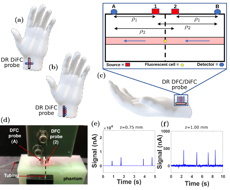
Figure 1: Conceptual application of Dual-Ratio (DR)Diffuse in-vivo Flow Cytometry (DiFC). In principle, source and detector pairs could be arranged (a) perpendicular, or (b) parallel to the underlying artery (in this case, the radial artery). (c) Use of two sources (1, 2) and two detectors (A, B) would permit four source and detector pairs separated by a source-detector distance ($\rho$). (d) Photograph of Near-InfraRed (NIR)Diffuse in-vivo Flow Cytometry (DiFC)system[pace_nearinfrareddiffusevivo_2022] on a diffusive flow phantom with fiber probes arranged perpendicular to the tubing direction. The dashed black line in (d) corresponds to the mid-plane shown in (c). The instrument permitted measurement with a single source and detector pair, in this case (2 & A). Background-subtracted sample DiFC data of fluorescent microspheres embedded (e) $0.75\text{\,}\mathrm{mm}$ deep and (f) $1.00\text{\,}\mathrm{mm}$ deep in a phantom with a flow channel.

1.2 Dual-Ratio

One of the most basic measurements in diffuse optics is that of the SD Reflectance ($R$), which is measured by placing a point source and a point detector on the surface of a highly scattering medium. In practice, the detector does not measure the theoretical $R$ but instead, some optical Intensity ($I$) that is proportional to the theoretical $R$ (Appendix LABEL:sec:app:noise:coup). The proportionality of $I$ to $R$ is controlled by Coupling coefficients ($C$s), which may be associated with the coupling efficiency of the optodes (sources or detectors) with the medium as well as any other multiplicative factor on $R$.

Recently, we introduced new measurement types that attempt to represent the theoretical $R$ by canceling any $C$s associated with optodes. These are the dual-slope[blaney_phasedualslopesfrequencydomain_2020] or the DR [blaney_methodmeasuringabsolute_2022] data types, which in their calculation cancel any multiplicative factors associated with optodes[blaney_functionalbrainmapping_2022, blaney_methodmeasuringabsolute_2022]. These measurement types essentially recover the spatial dependence of $R$ over multiple $\rho$s. This is achieved from a symmetrical optode arrangement of sources and detectors such as the one in Figure 1(c).

A further advantage of the dual-slope or DR data type is the reduced contribution to the signal from superficial parts of the diffuse medium[sassaroli_dualslopemethodenhanced_2019, fantini_transformationalchangefield_2019, blaney_phasedualslopesfrequencydomain_2020]. With the hypothesis that the unwanted AF contributors in DiFC measurements are mainly near the surface, we decided to explore if these data types could suppress the AF component of the DiFC measurement. We hypothesize that this AF suppression, together with the cancellation of noise through the cancellation of $C$s, will improve the SNR of DR over traditional SD DiFC measurements using NIR optical wavelengths ($\lambda$s). This improved SNR of DR DiFC could enable the detection of deep fluorescent targets, which is a current struggle of DiFC as discussed in Section 1.1. Therefore, this work investigates the potential of DR in the DiFC application and identifies the key parameters which control whether or not DR will be advantageous.

2 Methods

2.1 Proposed Dual-Ratio Signal

Most diffuse optical measurements recover an optical signal using a source and a detector, often each placed on a tissue surface. We consider each measurement of $I$ with a source and detector as a SD measurement (Appendix A.1). Previous DiFC work has considered these types of measurements[ivich_signalmeasurementconsiderations_2022]; however, in this work, we introduce a DiFC measurement type based on a combination of SDs to form a DR (Appendix A.3)[blaney_phasedualslopesfrequencydomain_2020, blaney_methodmeasuringabsolute_2022].

DR is defined in detail in Appendix A.3, and will be summarized here. The DR measurement is defined as follows:

$$\lx@glossaries@gls@link{acronym}{DR}{\leavevmode\text{DR}}=\sqrt{\frac{\lx@glossaries@gls@link{symbolslist}{I}{\leavevmode I}_{l,\text{{I}}}\lx@glossaries@gls@link{symbolslist}{I}{\leavevmode I}_{l,\text{{II}}}}{\lx@glossaries@gls@link{symbolslist}{I}{\leavevmode I}_{s,\text{{I}}}\lx@glossaries@gls@link{symbolslist}{I}{\leavevmode I}_{s,\text{{II}}}}}$$ (1)

where the $l$ and $s$ subscripts represent $I$ measurements at long or short $\rho$s, respectively. Additionally, the I and II subscripts show whether it is the first or second symmetric $I$ measurement in a DR. The exact geometric requirements for I and II are described in more detail in Appendix A.3 and previous publications (where DR is referred to as dual-slope, since geometric requirements for the two are the same)[blaney_designsourcedetector_2020]. For this work, consider Figure 1(c). In this case, $s$,I and $l$,I are detector A & source 1 (SD A1) and SD A2, respectively. And similarly, for detector B, $s$,II and $l$,II are SD B2 and SD B1, respectively.

2.2 Monte-Carlo Models

This work presents simulation results based on a Monte-Carlo (MC) model run in Monte-Carlo Extreme (MCXLAB 2020 running in MATLAB 2023a on an NVIDIA RTX 4090)[fang_montecarlosimulation_2009]. For all simulations optical properties meant to represent $\lambda$ of $810\text{\,}\mathrm{nm}$ were used[ivich_signalmeasurementconsiderations_2022]. These were an $\mu_{a}$ of $0.002\text{\,}{\mathrm{mm}}^{-1}$, a scattering coefficient ($\mu_{s}$) of $7\text{\,}{\mathrm{mm}}^{-1}$, an anisotropy factor ($g$) of $0.9$, and an index of refraction ($n$) of $1.37$. The MC was run by launching ${10}^{9}$ photons into a $$30\text{\,}\mathrm{mm}$\times$30\text{\,}\mathrm{mm}$\times$30\text{\,}\mathrm{mm}$$ volume, with grid spacing of $0.1\text{\,}\mathrm{mm}$ and $10$ time gates ending at $10\text{\,}\mathrm{ns}$. To calculate the Continuous-Wave (CW) $R$, the MC’s Time-Domain (TD) $R$ was integrated over the time gates.

For the coordinate system, the surface of the medium was considered to be $z=$0\text{\,}\mathrm{mm}$$ (positive $z$ pointing into the medium), and the center (with the edges $15\text{\,}\mathrm{mm}$ away in each direction) to be $x=$0\text{\,}\mathrm{mm}$$ and $y=$0\text{\,}\mathrm{mm}$$. Using this coordinate system, detector A was placed at $-3.5\hat{x}~{}$\mathrm{mm}$$, detector B at $3.5\hat{x}~{}$\mathrm{mm}$$, source 1 at $-0.5\hat{x}~{}$\mathrm{mm}$$, and source 2 at $0.5\hat{x}~{}$\mathrm{mm}$$. In the case of the $0\text{\,}\mathrm{mm}$ $\rho$ simulation, both source and detector were placed at the origin. A separate MC was run for each of these optodes to find the fluence rate ($\Phi$) distribution for a MC source placed at the optode position. This follows the adjoint method to calculate the $R$ for a given SD set[Yao_Biomed.Opt.ExpressBOE18_DirectApproach]. In the case of sources, a MC pencil beam was used, and in the case of detectors, a MC cone beam with a numerical aperture of $0.5$ was used to simulate the collection geometry of a fiber more accurately. This type of source distribution associated with the detectors is done to be closer to the condition of validity of the reciprocity theorem, which is crucial for applying the adjoint method. These $\Phi$s were used with Equation LABEL:equ:app:W to yield the fluorescence Jacobian ($W$) [ivich_signalmeasurementconsiderations_2022], a key parameter used in all the simulation results as described in Appendix B.

2.3 Experimental Measurements with Diffuse Flow Cytometry

2.3.1 Phantom Experiments with Fluorescent Microspheres In-Vitro

To estimate the potential performance of a DR DiFC instrument, we performed DiFC measurements in tissue-mimicking flow phantoms with NIR wavelengths ($770\text{\,}\mathrm{nm}$ excitation and $810\text{\,}\mathrm{nm}$ emission)[ivich_signalmeasurementconsiderations_2022]. Briefly, we used Jade Green High Intensity (JGHI, Spherotech Inc., Lake Forest, IL USA) cell-mimicking fluorescent microspheres (size approximately $10\text{\,}\mathrm{\SIUnitSymbolMicro m}14\text{\,}\mathrm{\SIUnitSymbolMicro m}$) for NIR SD measurements[pace_nearinfrareddiffusevivo_2022]. Microspheres were suspended at a concentration of ${10}^{3}\text{\,}{\mathrm{mL}}^{-1}$ in Phosphate Buffered Saline (PBS) and flowed through Tygon tubing (internal diameter of $0.25\text{\,}\mathrm{mm}$; TGY-010-C, Small Parts Inc., Seattle, WA USA) embedded in a tissue-mimicking optical flow phantom made of high-density polyethylene. Microsphere suspensions were pumped with a syringe pump (0-2209, Harvard Apparatus, Holliston, MA USA) at a flow rate of $50\text{\,}\mathrm{\SIUnitSymbolMicro L}\text{\,}{\mathrm{min}}^{-1}$, or average flow velocity of $17\text{\,}\mathrm{mm}\text{\,}{\mathrm{s}}^{-1}$ to approximate linear velocities in the mouse leg femoral artery.[patil_fluorescencemonitoringrare_2019, Hartmann_Phys.Med.Biol.17_FluorescenceDetection] The tubing at a depth of $1.50\text{\,}\mathrm{mm}$ in the phantom.

We performed SD DiFC measurements using a $\rho$ of $3\text{\,}\mathrm{mm}$ (Figure 1(c) $\lx@glossaries@gls@link{symbolslist}{rho}{\leavevmode\rho}_{1}$). Two fiber bundle probes were used, one as a source fiber and the other as a detector fiber. We collected DiFC data for the source (labeled as numbers) and detector (labeled as letters) pairs A1 and B2. To test the effect of the geometric arrangement of the probes relative to the flow tube, we performed measurements in the perpendicular or parallel directions as in Figure 1(a)(b). For illustration, a photograph of the A2 (at $\lx@glossaries@gls@link{symbolslist}{rho}{\leavevmode\rho}_{2}=$4\text{\,}\mathrm{mm}$$) SD NIR DiFC measurement is included in Figure 1(d), which shows a perpendicular placement of the probes to the tubing.

We collected $15\text{\,}\mathrm{min}$ DiFC scans and processed the data as described previously[tan_vivoflowcytometry_2019]. First, we performed background subtraction using a $5\text{\,}\mathrm{s}$ moving median window. Transit fluorescent peaks were measured as fluorescent microspheres were detected with the DiFC system. Here, peaks were defined as having a minimum amplitude of five times the noise (standard deviation of the data in a $1\text{\,}\mathrm{min}$ moving window). We analyzed peak amplitude, width (i.e., shape), and noise properties. These parameters were used in Appendix LABEL:sec:app:expPar to find the important parameters of fluorescence efficiency ($\eta$) and fluorescent $\mu_{a}$ needed to simulate SNR of DiFC measurements from the MC output.

2.3.2 Measurement of In-Vivo Autofluorescence on Mice

As discussed in more detail in Section 4.1 and Appendix LABEL:sec:app:expPar:bck, knowledge of the distribution of sources of AF is necessary for building a computational model of DR DiFC noise and background. To address this, we measured the AF background DiFC signal of the shaved inner thigh of recently euthanized mice: (1) at the surface of the skin and (2) at the surface of the exposed underlying muscle (without skin).

We used $N=$4$$ female BALB/c mice on a low-fluorescence chow diet for this experiment. The hair of the inner left thigh of these euthanized mice was removed with depilatory cream (Nair, Church & Dwight Co., Inc., Ewing, NJ). The skin of the right inner thigh was surgically removed, exposing the underlying muscle. We used our red DiFC instrument[tan_vivoflowcytometry_2019] to measure the background tissue AF background SD signal in both cases. During these measurements, ultrasound gel was applied between the DiFC probe and the tissue surface to minimize the index of refraction mismatch. DiFC was performed for $15\text{\,}\mathrm{min}$, and the mean background (i.e., with and without skin) was calculated from the resulting data.

3 Results

3.1 Monte-Carlo Simulated Maps & Signals

In Figure 2, we show the simulated SNR from a fluorescent target placed anywhere on the $y=$0\text{\,}\mathrm{mm}$$ plane. This shows which possible target positions would yield a measurable signal (SNR greater than one) and how strong the signal would be. One striking result that may be drawn from comparing the overall extent of the region with SNR greater than one for the case with surface-weighted contributions of AF (Figure 2(a)-(d)) and the case with homogeneous contributions (Figure 2(e)-(h)). In general, the case of homogeneous contributions of AF favors the shorter $\rho$s. It also severely weakens the ability of DR to measure targets when they are deep within the medium. In-fact, close examination of Figure 2(f)&(g) suggests that, counter-intuitively, a shorter $\rho$ can measure deeper. However, this is only evident in the homogeneous AF contributors case and not in the surface-weighted case. Thus telling us that the advantages of one measurement type over another depend on the spatial distribution of AF contributors.

We may also compare the different $\rho$s and the SD versus DR. For a $0\text{\,}\mathrm{mm}$ $\rho$, we see a small bulb shape close to the surface, confirming what is expected for a co-localized source and detector. The non-zero $\rho$s for SD show the typical banana shape expected in diffuse optics but with some differences. These differences arise from the small length scale used in these simulations, on the order of $1\text{\,}\mathrm{mm}$ so that the light does not act fully diffuse. For this reason, the MC source model matters much for the shape of the banana. To be more realistic, we modeled the source as a pencil beam and the detector as a cone with $0.5$ numerical aperture. This resulted in one side of the banana (the one near the source) being deeper than the other since the pencil beam could more effectively launch photons along the $z$ direction into the medium. These observations show that the MC source condition simulated matters and should match reality.

Focusing on DR, we see that it can measure deeper than every other measurement in the surface-weighted AF contributors case. However, in the homogeneous case, it does no better than the long ($\rho$ of $4\text{\,}\mathrm{mm}$) SD. This is primarily because DR focuses on canceling out signals from close to the surface. Therefore, it is advantageous when the confounding signal’s contributors, the AF’s chromophore concentration or efficiency, is surface weighted. This further reinforces the importance of understanding the distribution of AF in a realistic measurement case, like tissue, since it heavily affects which measurement type is preferable when detecting deep fluorescent targets.

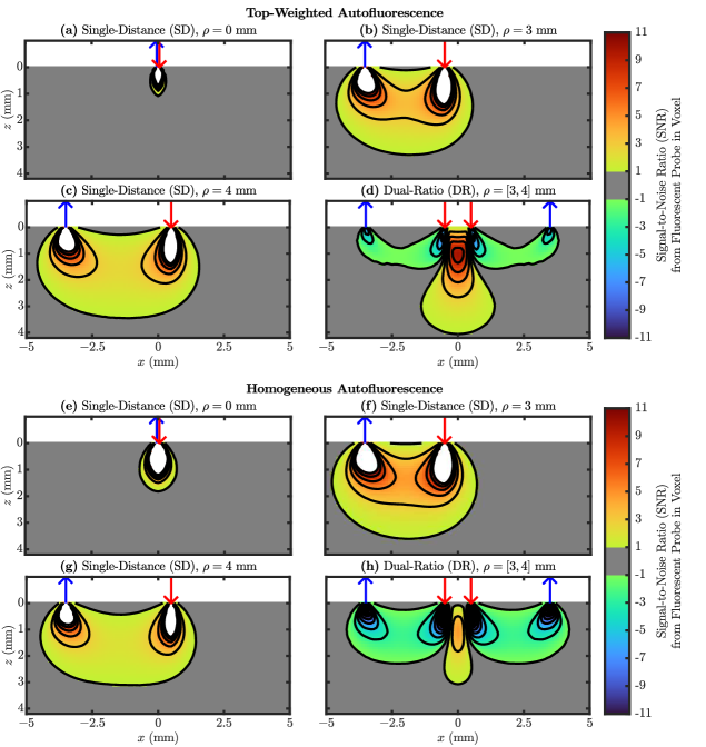
Figure 2: Map of the Signal-to-Noise Ratio (SNR)to a fluorescent target at a particular position (in the $y=$0\text{\,}\mathrm{mm}$$ plane) within a medium with surface-weighted ((a)-(d)) or homogeneous ((e)-(h)) AutoFluorescence (AF)contributors for four different measurement types with detectors represented by blue arrows and sources by red arrows. (a),(e) Single-Distance (SD)at a source-detector distance ($\rho$)of $0\text{\,}\mathrm{mm}$. (b),(f) SD at a $\rho$ of $3\text{\,}\mathrm{mm}$. (c),(g) SD at a $\rho$ of $4\text{\,}\mathrm{mm}$. (d),(h) Dual-Ratio (DR)containing $\rho$s of $3\text{\,}\mathrm{mm}4\text{\,}\mathrm{mm}$.
Note: White regions represent SNR greater than the maximum color-bar scale (i.e., 11) and gray regions represent absolute SNR less than one.
Parameters: Source = pencil, Detector = $0.5\text{\,}\mathrm{N}\mathrm{A}$ cone, voxel = $$0.1\text{\,}\mathrm{mm}$\times$0.1\text{\,}\mathrm{mm}$\times$0.1\text{\,}\mathrm{mm}$$, absorption coefficient ($\mu_{a}$) = $0.002\text{\,}{\mathrm{mm}}^{-1}$, scattering coefficient ($\mu_{s}$) = $7\text{\,}{\mathrm{mm}}^{-1}$, anisotropy factor ($g$) = $0.9$, index of refraction ($n$) = $1.37$, for surface-weighted ((a)-(d)) AF fluorescence efficiency ($\eta$) $\propto e^{\ln{(0.5)}z/$0.1\text{\,}\mathrm{mm}$}$ for homogeneous ((e)-(h)) $\eta$ constant, & signal and noise parameters found in appendix Appendix LABEL:sec:app:expPar (in this simulation we assumed $5\text{\,}\mathrm{\char 37\relax}$ Non-Cancelable noise).

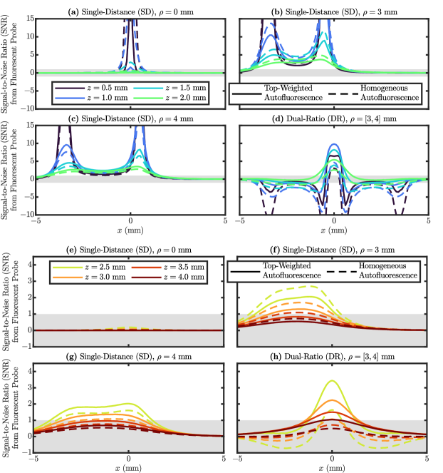
Figure 3: Traces of expected Signal-to-Noise Ratio (SNR)from a fluorescent target flowing at a particular depth (color) beneath the source-detector arrangement (same as Figure 1,2; $y=$0\text{\,}\mathrm{mm}$$). These results are shown for surface-weighted and homogeneous AF contributors (line-type). (a),(e) Single-Distance (SD)at a source-detector distance ($\rho$)of $0\text{\,}\mathrm{mm}$. (b),(f) SD at a $\rho$ of $3\text{\,}\mathrm{mm}$. (c),(g) SD at a $\rho$ of $4\text{\,}\mathrm{mm}$. (d),(h) Dual-Ratio (DR)containing $\rho$s of $3\text{\,}\mathrm{mm}4\text{\,}\mathrm{mm}$.
Note: Gray regions represent absolute SNR less than one.
Parameters: The same as Figure 2 with assumed $5\text{\,}\mathrm{\char 37\relax}$ Non-Cancelable noise.

In Figure 3, we present the expected signal profiles (in SNR) that one would measure if a fluorescent target flowed parallel to the source-detector line (in the $y=$0\text{\,}\mathrm{mm}$$ plane). The x-axis shows the $x$ coordinate; in an actual DiFC measurement, this would be time with the $x$ position scaled by the velocity. Different colors represent targets flowing at different depths, and line type shows the type of distribution of contributors to AF. The gray region shows where the absolute SNR is less than one, so if the curve drops into this region, we may say it is not measurable.

Many of the conclusions drawn from Figure 3 are similar to the ones that one may draw from Figure 2 since these traces (Figure 3) are simply line scans of Figure 2. So, we focus on more apparent features in these traces than the map. The first is the shape of a non-zero $\rho$ SD measurement. This is that of a double peak, which arises when the target first flows under the detector, making a strong signal, then under the source causing the target to make another strong signal. This is especially evident with shallow depths but is slightly present even in the broad traces simulated from deep $z$s. Further, because of the different MC source conditions, the peak height when the target passes under the source is higher than when the target passes under the detector. Therefore, we may say that this model predicts that a non-zero $\rho$ SD measurement will produce a rather unique signal, with a double peak and a more significant peak height when the target passes under the source.

Finally, lets examine the shape of the simulated DR signal (Figure 3(d),(h)). In this case, the signal has positive and negative components. Here it is essential to understand that these traces are differences from a baseline measurement, so that Figure 3(d),(h) shows the baseline DR subtracted from the current DR. This is detailed in Appendix A and Equation 8. Therefore negative values in the DR signal mean that the current DR value is less than the baseline value. Since one wishes to identify the presence of a fluorescent target, it does not matter whether the signal is positive or negative, so even SNR of DR less than $-1$ may be considered a signal which can identify the target. Knowing this, we see that the DR signal is unique and could further help identify if a target is genuinely detected. The DR signal is expected first to decrease as the target flows under the detector, then an increase when the target is under the source, followed by a decrease when the target finally flows under the second detector. Therefore, these results suggest that the DR (as well as the SD) signal has a unique shape that may be used to identify a true positive detection of the fluorescent target.

3.2 Comparison of Phantom Experiments and Simulated Signals

We collected experimental DiFC data using a phantom and fluorescent microspheres as described in Section 2.3.1. Figure 4 shows sample normalized and smoothed (with the shaded region showing noise) fluorescent microsphere peaks (i.e., detections) flowing $1.50\text{\,}\mathrm{mm}$ deep in a phantom. DiFC measurements from two SD pairs, A1 and B2, are shown in perpendicular (Figure 4(a)-(c)) and parallel (Figure 4(d)-(f)) probe to tube configurations. Normalization was performed to set the mean peak maximum of Figure 4(e)&(f) to one while using the same normalization factor for Figure 4(b)&(c). This allows for comparing the relative amplitudes between all traces in Figure 4.

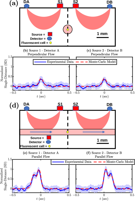
Figure 4: Traces showing a comparison of experimental phantom data and expected results from the Monte-Carlo (MC)model. Single-Distance (SD)traces are normalized so that the mean peak maximum between panels (e) and (f) is one, meaning all sub-panels utilize the same normalization factors. (a) Schematic of perpendicular flow case. (b),(c) Comparison for perpendicular flow case. (d) Schematic of parallel flow case. (e),(f) Comparison for parallel flow case.
Note: Shaded regions represent the noise level of the experimental data.
Parameters: The same as Figure 2 with a known of $1.5\text{\,}\mathrm{mm}$ and assumed fluorescent target velocity of $25\text{\,}\mathrm{mm}\text{\,}{\mathrm{s}}^{-1}$.

So that one may relate these normalized values to measured PhotoMultiplier Tube (PMT) currents, we provide the experimentally measured amplitudes for this data. For the parallel tube to probe configuration (Figure 4(e)-(f)), DiFC peak maximum amplitudes averaged $41\text{\,}\mathrm{nA}$ and $38\text{\,}\mathrm{nA}$ for A1 and B2, respectively. Meanwhile, for the perpendicular tube to probe configuration (Figure 4(a)&(c)), the peak amplitudes averaged $16.64\text{\,}\mathrm{nA}$ and $17.22\text{\,}\mathrm{nA}$ for 1A and 2B, respectively.

We have also overlaid normalized peaks simulated using MC (red dashed lines), using the same normalization method as the experimental data. This type of normalization ensures the mean amplitudes match experimental data for Figure 4(e)&(f) but does not ensure a match for Figure 4(b)&(c) or the individual amplitudes Figure 4(e)&(f). Additionally, the simulated velocity for the MC data was chosen to match the peak width with the experimental data. For this, a velocity of $25\text{\,}\mathrm{mm}\text{\,}{\mathrm{s}}^{-1}$ was used. However, since this velocity was assumed for all panels of Figure 4, a match to the peak width for an individual panel is not ensured. Therefore, a comparison between experimental data and MC simulations should be done against features that were not made to match. These features were the amplitude of the peaks in Figure 4(b)&(c), the amplitude of the lesser second peak in Figure 4(e)&(f), and the overall shape of the signal. With this in mind, we see excellent agreement between the MC simulations and experimental measurements. This is particularly true regarding the doublet peak shown in Figure 4(e)&(f), which is predicted by MC and observed experimentally. Note that the double peak in the parallel configuration is generated by the microsphere passing through high values of $W$ twice, once under the detector and once under the source. Additionally, the relative amplitudes of the doublet are influenced by the relationship between the numerical aperture of the source and detector, reinforcing the choice of a cone instead of a pencil beam for the detector in the MC simulation. In fact, if a pencil beam was chosen for both the source and detector MCs, the match to experimental data would be poor as the doublet peak would have the same maximum for both peaks in the doublet.

4 Discussion

4.1 Expected Depth

The primary reason for this work is to explore if the DR technique may be applied to DiFC. With this in mind, we must consider what metric to use to compare measurement methods such as SD versus DR. Since the aim of DiFC is to eventually non-invasively measure blood vessels of humans in-vivo, the maximum depth that a method can detect a fluorescent target is the metric which should be used for this comparison. One can determine this depth by examining Figure 2 and finding the deepest colored region for each data type. However, a line scan in $z$ of Figure 2, as shown in Figure 5, makes the relationships more apparent. The $x$ values chosen in Figure 5 were the centroid of the optodes (e.g. $-2.0\hat{x}~{}$\mathrm{mm}$$ for 1A); thus, the maximum measurable depth can be found by looking at where the curves in Figure 5 drop below a SNR of one (the gray region). Table 1 summarizes these maximum measurable depths. Note that a suitable vessel to measure in humans, such as the radial artery, is located approximately $2\text{\,}\mathrm{mm}4\text{\,}\mathrm{mm}$ deep[selvaraj_ultrasoundevaluationeffect_2016].

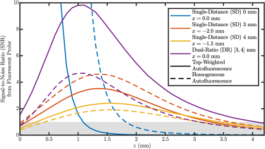
Figure 5: Signal-to-Noise Ratio (SNR)from a fluorescent target below the centroid of the optodes used for each measurement type as a function of depth ($z$). Colors show different measurement types, and line type shows the AutoFluorescence (AF)contributor distribution.
Parameters: The same as Figure 2 with assumed $5\text{\,}\mathrm{\char 37\relax}$ Non-Cancelable noise.

Table 1: Maximum Measurable Depths of Fluorescent Target for Different Measurement Types

	$\max[z[\text{\lx@glossaries@gls@link{acronym}{SNR}{\leavevmode SNR}}>1]]$ ($\mathrm{mm}$)
	SD $\rho$ =$0\text{\,}\mathrm{mm}$	SD $\rho$ =$3\text{\,}\mathrm{mm}$	SD $\rho$ =$4\text{\,}\mathrm{mm}$	DR $\rho$ s=[$3$, $4$] $\mathrm{mm}$
Surface-Weighted
AF Contributors	$1.0$	$3.2$	$3.4$	$4.0$
Homogeneous
AF Contributors	$1.8$	$3.6$	$3.1$	$3.0$

Acronyms: Signal-to-Noise Ratio (SNR), Single-Distance (SD), Dual-Ratio (DR), source-detector distance ($\rho$), & AutoFluorescence (AF).
Parameters: The same as Figure 2 with assumed $5\text{\,}\mathrm{\char 37\relax}$ Non-Cancelable noise.

As is evident in Table 1, the depth of DR is heavily affected by the AF contributor distribution. Specifically, if the AF contributor distribution is surface-weighted, DR is the best measurement type, while this is not true for homogeneous. Evidence suggests that the AF contributor distribution is surface-weighted in-vivo. To investigate the spatial distribution of the AF contributors, we measured the background signal of a mouse as described in Section 2.3.2. The mean background with skin was $17\,400\pm 3500\text{\,}\mathrm{nA}$, whereas the mean background of the bare muscle (without skin) was $9200\pm 540\text{\,}\mathrm{nA}$, which is a reduction of $47\text{\,}\mathrm{\char 37\relax}$. These results imply that DiFC AF is weighted to superficial tissue layers, and as discussed below, from what we can find in the literature, this seems to be the case qualitatively.

A literature search did not reveal a specific quantification of the spatial distribution of AF contributors. Nevertheless, the available literature on known endogenous fluorophores strongly suggests that these should be weighted more heavily in the skin. Specifically, reduced Nicotinamide Adenine Dinucleotide (NADH), Flavin Adenine Dinucleotide (FAD), collagen, and elastin fluoresce in the visible (violet and blue) wavelength regions[monici_celltissueautofluorescence_2005, croce_autofluorescencespectroscopyimaging_2014] and to a lesser degree in the red and NIR wavelength regions,[hong_nearinfraredfluorophoresbiomedical_2017, gibbs_infraredfluorescenceimageguided_2012] the latter being most relevant for the potential use of DR DiFC in humans[ivich_signalmeasurementconsiderations_2022]. Other significant contributors of tissue AF in the red and NIR wavelength regions are less obvious due to their rarity[thomas_identifyingnovelendogenous_2016]. Furthermore, AF in the red and NIR wavelength region may be more complex than visible AF because of the overall reduction in optical scattering and absorption at longer wavelengths[semenov_oxidationinducedautofluorescencehypothesis_2020]. However, we found lipofuscin,[marmorstein_spectralprofilingautofluorescence_2002] melanin,[huang_cutaneousmelaninexhibiting_2006, wang_vivonearinfraredautofluorescence_2013] and heme-metabolic compounds like porphyrins and bilirubin,[htun_nearinfraredautofluorescenceinduced_2017, lifante_roletissuefluorescence_2020] to be reported as auto-fluorescent in the red and NIR wavelength region, all of which are present in the skin. Bilirubin and other heme-metabolic products are mostly known for contributing to liver AF [demos_nearinfraredautofluorescenceimaging_2004]. However, in the context of DiFC, these compounds may accumulate in the skin from hematomas in the case of injury. Thus, the available literature and experimental DiFC measurements in mice (above) suggest that contributors to the background AF in the red and NIR wavelength region for potential DR DiFC are mostly in the skin as opposed to underlying tissue structures.

4.2 Consideration of Noise

The noise and signal level used in these simulations was based on experimental data collected at $3\text{\,}\mathrm{mm}$ SD (Appendix LABEL:sec:app:expPar). However, one noise parameter that cannot be derived from the collected experimental data is the correlation of the noise measured by different optodes. This correlation between optode noises does not affect the SD results but does significantly affect the DR results since it affects how the DR can cancel noise.

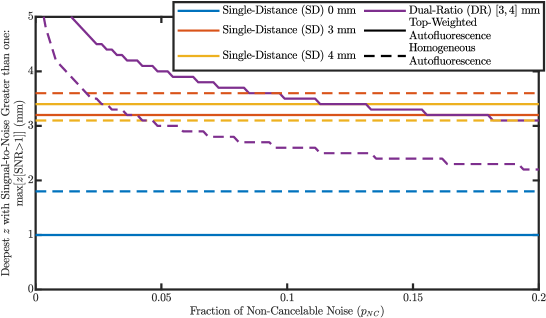
Figure 6: The deepest fluorescent target that each data type can measure (Signal-to-Noise Ratio (SNR)greater than one) as a function of the fraction of non-cancelable (by Dual-Ratio (DR)) noise ($p_{NC}$). Colors show the data type, and line type shows the distribution of AutoFluorescence (AF)contributors.
Note: For a definition of see Appendix LABEL:sec:app:noise or Equation 2. Parameters: The same as Figure 2.

We modeled noise as Gaussian random variables (Coupling coefficient random variable ($\mathcal{C}$)) that multiplied the theoretical $R$ to yield the measured Intensity random variable ($\mathcal{I}$) (Appendix LABEL:sec:app:noise). A separate independent random variable represents each optode (source or detector) and can be considered noise in the coupling, gain, power, or any other optode-specific noise. This concept, explained in detail in Appendix LABEL:sec:app:expPar, can be summarized by:

$$\begin{split}\lx@glossaries@gls@link{symbolslist}{Ir}{\leavevmode\mathcal{I}}(\lx@glossaries@gls@link{symbolslist}{R}{\leavevmode R},\lx@glossaries@gls@link{symbolslist}{sigmaI}{\leavevmode\sigma_{\lx@glossaries@gls@link{symbolslist}{I}{\leavevmode I}}}^{2})\simeq\hskip 284.52756pt\\ \lx@glossaries@gls@link{symbolslist}{Cr}{\leavevmode\mathcal{C}}_{\text{Source}}\left(1,p_{\text{Source}}\left(\frac{\lx@glossaries@gls@link{symbolslist}{sigmaI}{\leavevmode\sigma_{\lx@glossaries@gls@link{symbolslist}{I}{\leavevmode I}}}}{\lx@glossaries@gls@link{symbolslist}{R}{\leavevmode R}}\right)^{2}\right)\times\lx@glossaries@gls@link{symbolslist}{Cr}{\leavevmode\mathcal{C}}_{\text{Detector}}\left(1,p_{\text{Detector}}\left(\frac{\lx@glossaries@gls@link{symbolslist}{sigmaI}{\leavevmode\sigma_{\lx@glossaries@gls@link{symbolslist}{I}{\leavevmode I}}}}{\lx@glossaries@gls@link{symbolslist}{R}{\leavevmode R}}\right)^{2}\right)\times\\ \lx@glossaries@gls@link{symbolslist}{Cr}{\leavevmode\mathcal{C}}_{NC}\left(1,p_{NC}\left(\frac{\lx@glossaries@gls@link{symbolslist}{sigmaI}{\leavevmode\sigma_{\lx@glossaries@gls@link{symbolslist}{I}{\leavevmode I}}}}{\lx@glossaries@gls@link{symbolslist}{R}{\leavevmode R}}\right)^{2}\right)\times\lx@glossaries@gls@link{symbolslist}{R}{\leavevmode R}\end{split}$$ (2)

where,

$$p_{\text{Source}}+p_{\text{Detector}}+p_{NC}=1$$ (3)

using the random variable notation where the first argument is the mean and the second the variance. Since $\lx@glossaries@gls@link{symbolslist}{sigmaI}{\leavevmode\sigma_{\lx@glossaries@gls@link{symbolslist}{I}{\leavevmode I}}}/\lx@glossaries@gls@link{symbolslist}{R}{\leavevmode R}\ll 1$, the I defined by the right hand side of Equation 2 is an excellent approximation of a random variable with mean R and variance $\lx@glossaries@gls@link{symbolslist}{sigmaI}{\leavevmode\sigma_{\lx@glossaries@gls@link{symbolslist}{I}{\leavevmode I}}}^{2}$ ($\lx@glossaries@gls@link{symbolslist}{Ir}{\leavevmode\mathcal{I}}(\lx@glossaries@gls@link{symbolslist}{R}{\leavevmode R},\lx@glossaries@gls@link{symbolslist}{sigmaI}{\leavevmode\sigma_{\lx@glossaries@gls@link{symbolslist}{I}{\leavevmode I}}}^{2})$). The DR cancels all $\mathcal{C}$s associated with specific optodes (Equation LABEL:equ:app:DRwC) but not the Non-Cancelable ($NC$) $\mathcal{C}$. $NC$ is named such since it is the noise not canceled by DR. From this, we see that the parameter controlling the amount of noise that propagates into DR is $p_{NC}$, which is the fraction of the variance which is non-cancelable by DR.

In all the above results in this work, $p_{NC}$ was assumed to be $5\text{\,}\mathrm{\char 37\relax}$. Note that we do not know the physical origin of this noise if all SDs are acquired simultaneously, so we apply this noise to noise introduced from multiplexing. We expect that advanced multiplexing schemes may alleviate this noise (Section 4.3), but do not know what it is for the current system, so we assumed what we consider a reasonable value of $5\text{\,}\mathrm{\char 37\relax}$.

To experiment with the effect of $p_{NC}$, we varied its value and determined the maximum measurable depth (where SNR is greater than one) for each data type in Figure 6. Note that all SD measurements experience the same noise regardless of $p_{NC}$’s value, and only DR is affected. This is because the model was designed so that the total noise is the same regardless of the $p_{NC}$ value. From Figure 6, we can find the allowable $p_{NC}$, which makes DR sense deeper than the deepest SD modeled. For the simulation with surface-weighted AF contributions, this is $12\text{\,}\mathrm{\char 37\relax}$, while for the homogeneous case, it is $2\text{\,}\mathrm{\char 37\relax}$. This further emphasizes the advantage DR has in the surface-weighted AF medium. Additionally, this guides the amount of $p_{NC}$, which a system can have for DR to have an advantage over SD.

4.3 Future Implementation

The experimental and computational data presented here were based on measurements using SD or SR (not presented for brevity) measurements taken in series using our existing DiFC instrument[tan_vivoflowcytometry_2019, pace_nearinfrareddiffusevivo_2022]. In practice, implementation of a DR for DiFC would require the construction of a new DiFC instrument capable of making simultaneous measurements with two sources and two detectors as in Figure 1(c). Several optical designs would enable this. For example, we could frequency encode the two laser sources by modulating them at different frequencies and de-modulating the fluorescence signals measured by the two detectors to separate the contributions from the two sources (frequency-multiplexing). Likewise, we could alternately illuminate the two laser sources (S1 and S2) in an on-off pattern (time-multiplexing). Assuming a peak width of $10\text{\,}\mathrm{ms}$ in-vivo[tan_vivoflowcytometry_2019], this should be achievable by time-multiplexing the laser output at about $1\text{\,}\mathrm{kHz}$.

Fast time-multiplexing or frequency-multiplexing would be desirable because the DR strategy would inherently cancel out signal drift and noise. DR cancelable artifacts are associated with a multiplicative factor applied to a source or detector that does not change within the multiplexing cycle (Appendix LABEL:sec:app:noise:coup). This could include instrument drift or coupling of the sources and detectors to the skin surface. However, this approach cannot cancel some sources of random noise in the signal (Appendix LABEL:sec:app:noise:coup & Figure 6). In principle, using modulated laser sources and lock-in detection for frequency-multiplexing would improve the SNR of detected peaks in the presence of non-cancellable noise. Furthermore, as shown in Figures 3&4, the DR DiFC measurement using a parallel configuration (Figure 1(b)) yielded a unique double-peak shape. Therefore, we expect that using matched filters (or machine learning methods based on signal temporal shape) could improve peak detection. DR noise would also be suppressed when the two $\rho$s are as different as possible[blaney_designsourcedetector_2020]. Therefore, custom-designed optical fiber bundles may be convenient for delivering and collecting light in a DR DiFC instrument. For instance, we can design a new DiFC optical fiber bundle that incorporates multiple source fibers with symmetric separations and large detector areas.

Finally, we note that this work is the first case of dual-slope / DR applied to fluorescence in general, not only to DiFC. dual-slope / DR was first developed for NIR Spectroscopy (NIRS) and measurement of changes in $\mu_{a}$ ($\Delta\mu_{a}$) [sassaroli_dualslopemethodenhanced_2019, blaney_phasedualslopesfrequencydomain_2020]. Now, with the methods presented in this work, we believe dual-slope / DR may also be applied to diffuse fluorescence spectroscopy and tomography[htun_nearinfraredautofluorescenceinduced_2017, grosenick_reviewopticalbreast_2016, croce_autofluorescencespectroscopyimaging_2014, wang_deeptissuefocalfluorescence_2012, klose_inversesourceproblem_2005, georgakoudi_trimodalspectroscopydetection_2002]. dual-slope / DR should lend itself well to any application which aims to measure changes in fluorescence (i.e., instead of $\Delta\mu_{a}$ as it was used for in NIRS). Thus, we open the door to future work regarding dual-slope / DR fluorescence.

5 Conclusion

This work explored the feasibility of using DR for DiFC. We accomplished this by running MC models of the expected DR SNR based on noise and fluorescence parameters extracted from experimental DiFC data. From this exploration, we modify two key factors which control whether DR is beneficial to DiFC or not. The first is the distribution of AF contributors in-vivo, with surface-weighted giving DR methods an advantage. Experiments on mice and a literature search suggest that the in-vivo AF contributor distribution is concentrated in the skin, suggesting that DR will have an advantage over traditional SD methods. The second key parameter is the portion of non-cancellable (by DR) noise in the measurement. This noise is not associated with multiplicative optode factors (e.g. tissue coupling, source power, or detector efficiency), which are constant within a multiplexing cycle. A DiFC instrument designed for DR would need to be built to explore and address this. A future DiFC instrument may achieve the DR measurement by time- or frequency-multiplexing leading to the required level of non-cancelable noise. Therefore, this work laid the groundwork to identify the key parameters of concern and aid in designing a DR DiFC instrument.

Appendix A Definition of Measurement Types

A.1 Single-Distance

The raw measurement from a Diffuse in-vivo Flow Cytometry (DiFC) system is the Intensity ($I$) measured between a source and a detector which we also refer to as the Single-Distance (SD) here. Using this raw measurement we define the change in the SD ($\Delta\text{SD}$) as the background-subtracted $I$ as follows:

$$\lx@glossaries@gls@link{symbolslist}{dSD}{\leavevmode\Delta\text{SD}}(\lx@glossaries@gls@link{symbolslist}{t}{\leavevmode t})=\lx@glossaries@gls@link{symbolslist}{I}{\leavevmode I}(t)-\lx@glossaries@gls@link{symbolslist}{I}{\leavevmode I}_{0}$$ (4)

where, $\Delta\text{SD}$ is expressed as a function of time ($t$) and $\lx@glossaries@gls@link{symbolslist}{I}{\leavevmode I}_{0}$ is the average or $I$ over a baseline $t$. $\lx@glossaries@gls@link{symbolslist}{I}{\leavevmode I}_{0}$ could be found in various ways, for example: based on an initial measurement or an average over a preceding time period, regardless $\Delta\text{SD}$ represents a change in $I$ over $t$. Here, the primary measurement parameter is the source-detector distance ($\rho$), in this work SDs are evaluated at $\rho$ of either $3\text{\,}\mathrm{mm}$ or $4\text{\,}\mathrm{mm}$.

A.2 Single-Ratio

Next we define the Single-Ratio (SR) which is a ratio of $I$s measured at long and short $\rho$s:

$$\lx@glossaries@gls@link{acronym}{SR}{\leavevmode\text{SR}}=\frac{\lx@glossaries@gls@link{symbolslist}{I}{\leavevmode I}_{l}}{\lx@glossaries@gls@link{symbolslist}{I}{\leavevmode I}_{s}}$$ (5)

where, the $l$ or $s$ subscripts represent measurements at either long or short $\rho$s, respectively. Using Equation 5 we next express the change in the SR ($\Delta\text{SR}$):

$$\lx@glossaries@gls@link{symbolslist}{dSR}{\leavevmode\Delta\text{SR}}(\lx@glossaries@gls@link{symbolslist}{t}{\leavevmode t})=\frac{\lx@glossaries@gls@link{symbolslist}{I}{\leavevmode I}_{l}(\lx@glossaries@gls@link{symbolslist}{t}{\leavevmode t})}{\lx@glossaries@gls@link{symbolslist}{I}{\leavevmode I}_{s}(\lx@glossaries@gls@link{symbolslist}{t}{\leavevmode t})}-\frac{\lx@glossaries@gls@link{symbolslist}{I}{\leavevmode I}_{l,0}}{\lx@glossaries@gls@link{symbolslist}{I}{\leavevmode I}_{s,0}}$$ (6)

which, as with $\Delta\text{SD}$, is also expressed as a function of time. The primary parameters for SR are the long and short $\rho$s which are $3\text{\,}\mathrm{mm}$ and $4\text{\,}\mathrm{mm}$ in this work.

A.3 Dual-Ratio

Finally, we define the Dual-Ratio (DR), which is the geometric mean of two SRs related through geometric requirements. These requirements can be summarized by stating that optodes that contribute to the short $\rho$ for one SR contribute to the long $\rho$ for the other SR in a DR; and vice-versa. Suppose we have two SRs named $\lx@glossaries@gls@link{acronym}{SR}{\leavevmode\text{SR}}_{\text{{I}}}$ and $\lx@glossaries@gls@link{acronym}{SR}{\leavevmode\text{SR}}_{\text{{II}}}$. Naming sources as numbers and detectors as letters, we can say that $\lx@glossaries@gls@link{acronym}{SR}{\leavevmode\text{SR}}_{\text{{I}}}$ contains one detector (A) and two sources (1 & 2) such that the short $\rho$ is obtained between 1 & A and the long $\rho$ between 2 & A (Figure 1(d)). Now consider $\lx@glossaries@gls@link{acronym}{SR}{\leavevmode\text{SR}}_{\text{{II}}}$ to be made of detector B and the same two sources 1 & 2 with the short $\rho$ being between B & 2 and the long $\rho$ between B & 1. Now notice that for $\lx@glossaries@gls@link{acronym}{SR}{\leavevmode\text{SR}}_{\text{{I}}}$ 1 forms the short $\rho$ but for $\lx@glossaries@gls@link{acronym}{SR}{\leavevmode\text{SR}}_{\text{{II}}}$ 1 forms the long $\rho$. Similarly for $\lx@glossaries@gls@link{acronym}{SR}{\leavevmode\text{SR}}_{\text{{II}}}$ 2 forms the short $\rho$ but for $\lx@glossaries@gls@link{acronym}{SR}{\leavevmode\text{SR}}_{\text{{I}}}$ 2 forms the long $\rho$. Therefore the geometric requirements are satisfied, and the geometric mean of $\lx@glossaries@gls@link{acronym}{SR}{\leavevmode\text{SR}}_{\text{{I}}}$ & $\lx@glossaries@gls@link{acronym}{SR}{\leavevmode\text{SR}}_{\text{{II}}}$ form a DR:

$$\lx@glossaries@gls@link{acronym}{DR}{\leavevmode\text{DR}}=\sqrt{\lx@glossaries@gls@link{acronym}{SR}{\leavevmode\text{SR}}_{\text{{I}}}\lx@glossaries@gls@link{acronym}{SR}{\leavevmode\text{SR}}_{\text{{II}}}}=\sqrt{\frac{\lx@glossaries@gls@link{symbolslist}{I}{\leavevmode I}_{l,\text{{I}}}\lx@glossaries@gls@link{symbolslist}{I}{\leavevmode I}_{l,\text{{II}}}}{\lx@glossaries@gls@link{symbolslist}{I}{\leavevmode I}_{s,\text{{I}}}\lx@glossaries@gls@link{symbolslist}{I}{\leavevmode I}_{s,\text{{II}}}}}$$ (7)

and thus change in the DR ($\Delta\text{DR}$) can we written as:

$$\lx@glossaries@gls@link{symbolslist}{dDR}{\leavevmode\Delta\text{DR}}(\lx@glossaries@gls@link{symbolslist}{t}{\leavevmode t})=\sqrt{\frac{\lx@glossaries@gls@link{symbolslist}{I}{\leavevmode I}_{l,\text{{I}}}(\lx@glossaries@gls@link{symbolslist}{t}{\leavevmode t})\lx@glossaries@gls@link{symbolslist}{I}{\leavevmode I}_{l,\text{{II}}}(\lx@glossaries@gls@link{symbolslist}{t}{\leavevmode t})}{\lx@glossaries@gls@link{symbolslist}{I}{\leavevmode I}_{s,\text{{I}}}(\lx@glossaries@gls@link{symbolslist}{t}{\leavevmode t})\lx@glossaries@gls@link{symbolslist}{I}{\leavevmode I}_{s,\text{{II}}}(\lx@glossaries@gls@link{symbolslist}{t}{\leavevmode t})}}-\sqrt{\frac{\lx@glossaries@gls@link{symbolslist}{I}{\leavevmode I}_{l,\text{{I}},0}\lx@glossaries@gls@link{symbolslist}{I}{\leavevmode I}_{l,\text{{II}},0}}{\lx@glossaries@gls@link{symbolslist}{I}{\leavevmode I}_{s,\text{{I}},0}\lx@glossaries@gls@link{symbolslist}{I}{\leavevmode I}_{s,\text{{II}},0}}}$$ (8)

Similarly to SR the parameters that are important for DR are the short and long $\rho$s. However, in this case, there are two short and two long $\rho$s. In this work both short are considered to be $3\text{\,}\mathrm{mm}$ and both long $4\text{\,}\mathrm{mm}$.

Appendix B Theory

B.1 Modeling Fluorescent Reflectance

To model the detected fluorescent Reflectance ($R$) we must consider two processes. First, the delivery of power to the fluorophores. Second, the transport of emitted light from the fluorophores to the detector.

B.1.1 Dependence on Fluorophore Position

The expression for the power volume density ($Q$) absorbed by a fluorophore ($\lx@glossaries@gls@link{symbolslist}{Q}{\leavevmode Q}_{fl,ab}(\lx@glossaries@gls@link{symbolslist}{r}{\leavevmode\vec{r}}_{fl})$; unit of $\mathrm{mW}\text{\,}{\mathrm{mm}}^{-3}$) at the position vector ($\vec{r}$) of the fluorophore ($\lx@glossaries@gls@link{symbolslist}{r}{\leavevmode\vec{r}}_{fl}$) can be written as:

$$\text{<span title="" class="ltx\_glossaryref ltx\_font\_italic">Q</span>}{}_{fl,ab}(\text{<span title="" class="ltx\_glossaryref ltx\_font\_italic">→r</span>}{}_{fl})=\text{<span title="" class="ltx\_glossaryref ltx\_font\_italic">Φ</span>}(\text{<span title="" class="ltx\_glossaryref ltx\_font\_italic">→r</span>}{}_{src}\to \text{<span title="" class="ltx\_glossaryref ltx\_font\_italic">→r</span>}{}_{fl})\text{<span title="" class="ltx\_glossaryref"><span class="ltx\_text ltx\_glossary\_name"><xmath xmlns="http://dlmf.nist.gov/LaTeXML" id="A2.E9.m1.1.16d" xref="A2.E9.m1.1.16i.cmml"><xmtok name="mu" role="UNKNOWN" font="italic" id="A2.E9.m1.1.16e" xref="A2.E9.m1.1.16i.cmml">μ</xmtok><xmapp role="POSTSUBSCRIPT" scriptpos="1" id="A2.E9.m1.1.16f" xref="A2.E9.m1.1.16i.cmml"><xmarg rule="Subscript" id="A2.E9.m1.1.16g" xref="A2.E9.m1.1.16i.cmml"><xmtok role="UNKNOWN" fontsize="70\%" font="italic" id="A2.E9.m1.1.16h" xref="A2.E9.m1.1.16i.cmml">a</xmtok></xmarg></xmapp></xmath></span></span>}$$ (9)