Stabilization of Discrete Time-Crystaline Response on a Superconducting Quantum Computer by increasing the Interaction Range

Abstract

This work presents a novel method for reproducing the dynamics of systems with couplings beyond nearest neighbors using a superconducting quantum processor. Quantum simulation of complex quantum many-body systems is a promising short-term goal of noisy intermediate-scale quantum (NISQ) devices. However, the limited connectivity of native qubits hinders the implementation of quantum algorithms that require long-range interactions. We show that utilizing the universality of quantum processor native gates allows the implementation of couplings among physically disconnected qubits. To demonstrate the effectiveness of our method, we implement a quantum simulation, on IBM quantum superconducting processors, of a Floquet-driven quantum spin chain featuring interactions beyond nearest neighbors. Specifically, we benchmark the prethermal stabilization of discrete Floquet time crystalline response as the interaction range increases, a phenomenon which was never experimentally observed before. Our method enables the study of systems with tunable interaction ranges, opening up new opportunities to explore the physics of long-range interacting quantum systems.

Introduction

Quantum computers are a revolutionary technology that have the potential to transform our society by solving problems that classical computers cannot [1]. However, these machines are still subject to uncontrollable noise and errors that limit their performance, which are far from the threshold required for error correction. Despite these limitations, recent progress in the realm of noisy intermediate-scale quantum (NISQ) devices represents an exciting opportunity for many-body physics by introducing new laboratory platforms with unprecedented control and measurement capabilities [2]. Quantum simulation of the dynamics of more and more complex quantum many-body systems is expected to be one of the most promising short-term goals of NISQ quantum computing devices, with intriguing applications in diverse areas ranging from quantum chemistry [3, 4, 5] and material science [6] to high-energy physics [7].

Various experimental platforms have been tested for quantum computing, among the others we can cite: trapped ions [8, 9, 10, 11], neutral Rydbger atoms [12, 13, 14], coherent photons [15, 16], nuclear spins in molecule [17, 18], NV centers [19, 20, 21] and superconducting qubits [22, 23]. Each of them has its own advantages and drawbacks [24]. In this paper, we focus on superconducting quantum processors. Superconducting qubits are relatively easy to fabricate and can be densely packed, allowing for the construction of large-scale quantum computers. This makes them a promising platform for scaling up quantum computing applications [25]. Moreover they can be manipulated with a wide range of microwave frequencies, making them versatile and flexible for implementing various quantum gates [22].

Thanks to this flexibility, the number of quantum simulations implemented on noisy superconducting devices has steadily risen in recent years, also thanks to the possibility to easily access these machines from remote, allowing to benchmark a number of phenomena which were not or were very little experimentally corroborated before. Among this plethora of studies we may mention the following: the observation of disorder stabilized discrete time crystal phases [26, 27], the realization of topologically ordered states, dynamical topological phases and topological edge states [28, 29, 30]. One should also cite the observation of Leggett-Garg’s inequalities violations [31], the validation of dynamical scalings [32, 33] and several studies in the context of quantum thermodynamics  [34, 35, 36]. On the other hand, the performance of superconducting NISQ devices is limited by the presence of various sources of noise and decoherence, whose impact grows with the depth and complexity of the quantum circuit realized, limiting the investigation of non-local effects and complex geometries.

Long-range interactions are known to boost the performance of quantum hardware [37, 38, 39, 40] as they evade the traditional constraint imposed by thermal equilibration and noise propagation. The stability of long-range quantum systems against external perturbations [41] and their role as a source of unprecedented phenomena, including novel forms of dynamical phase transitions and defect formation [42, 43, 44, 45], anomalous thermalization and information spreading [46, 47, 48, 49], metastable phases [50, 51], and entanglement scalings [52, 53] have been widely proven [54, 41]. However, the theoretical comprehension of such behaviors is still mainly limited to integrable quadratic systems or perturbations of fully connected mean-field models, while systems with a tunable interaction range require an extremely high degree of experimental control [54].

In this context, one main limitation of superconducting NISQ devices is their extremely limited connectivity, since superconducting qubits are typically arranged in a one or two-dimensional grid with nearest-neighbor connectivity, making it challenging to implement quantum algorithms that require long-range interactions [1]. In this paper, we aim to advance the field of digital quantum simulation on superconducting quantum hardware by investigating the possibility of reproducing the dynamics of systems with couplings beyond nearest neighbors. To achieve this, we utilize the universality of the quantum processor native gates to implement couplings among physically unconnected qubits. While the depth of the resulting quantum circuit increases with the effective range of the interaction, we show that careful consideration of gate noise, measurement errors, and statistical errors enables the removal of their effects from the raw results. The resulting error mitigated closely reproduce the theoretical expectations.

As a test bed for our general method, we implement the quantum simulation of a Floquet driven quantum spin chain featuring interactions beyond nearest neighbors on IBM quantum superconducting processors. Indeed, the quantum circuit structure utilized by IBMQ quantum computers is well-suited for implementing discrete Floquet driving protocols [2], making it a natural choice for such applications [27].

Our focus is on the stabilization of discrete Floquet time crystalline response as the interaction range increases. Discrete Floquet time crystals (DFTC) are non-equilibrium many-body phases of matter that display a novel form of spatiotemporal order. In particular, in such phases the discrete time translation symmetry of the Floquet driving is broken and an order parameter exhibits persistent oscillations with a period which is an integer multiple of the period of the drive [55, 56, 57, 58, 59, 60, 61, 62, 63, 64]. The possibility of generating a DFTC in clean systems has been studied in the context of LR interacting models, and our quantum simulation on IBM quantum processors constitutes its first experimental benchmark. Our results demonstrate the potential of superconducting quantum computing platforms to simulate quantum systems featuring interaction ranges going beyond the limits imposed by hardware connectivity and offer insights into the fundamental physics of long-range systems.

The Kicked Ising Chain with Long-Range Interactions

The Kicked Ising Spin Chain is a prototypical model for the investigation of Floquet driven quantum systems, widely studied from a theoretical point of view [65, 66, 67, 68, 69]. In this paper, we consider a driven quantum spin chain described by a time-dependent Hamiltonian of the form

$$H(t)=-\sum_{j=1}^{N}\sum_{r=1}^{R}J_{r}Z_{j}Z_{j+r}+h(t)\sum_{j=0}^{N-1}X_{j},$$ (1)

where the time dependence is generated by a time periodic driving with period $T$ of the transverse magnetic field $h(t)$. The driving takes the form:

$$h(t)=\phi\sum_{n=1}^{\infty}\delta(t-nT),$$ (2)

The effect of this impulsive magnetic field applied at integer multiples of the driving period $t=nT$ is to impose a global rotation of every spin by an angle $2\phi$ along the $x$-axis. Accordingly, the Floquet dynamics is obtained by periodically intertwining the evolution generated by the Ising Hamiltonian at zero transverse field

$$V=\prod_{j=1}^{N}\prod_{r=1}^{R}e^{iTJ_{r}Z_{j}Z_{j+r}},$$ (3)

with the instantaneous kick operator:

$$K_{\phi}=\prod_{j=1}^{N}e^{-i\phi X_{j}}.$$ (4)

The resulting evolution operator for a single step of the Floquet protocol reads

$$U_{F}=K_{\phi}V.$$ (5)

The system is initialized at $t=0$ in the fully polarized state with positive magnetization along the $\hat{z}$ direction:

$$\left|\psi(0)\right\rangle=\left|\dots\uparrow\uparrow\uparrow\dots\right\rangle=\left|\dots 000\dots\right\rangle,$$ (6)

where $\left|\uparrow\right\rangle$ and $\left|\downarrow\right\rangle$ denote the eigenstates of the $Z$ Pauli matrix with eigenvalues $+1$ and $-1$ respectively. In our case, these eigenstates correspond to the computational basis of the quantum processor, with the convention $\left|\uparrow\right\rangle=\left|0\right\rangle$ and $\left|\downarrow\right\rangle=\left|1\right\rangle$.

The simplest realization of the time-crystalline spatiotemporal order is obtained by taking the kick operator $K_{\phi}$ to rotate each spin by an angle $\pi$ around a transverse axis $\hat{x}$. In this case, the kick operator is given by

$$K_{\pi/2}=\prod_{j=1}^{N}e^{-i\frac{\pi}{2}X_{j}}=\prod_{j=1}^{N}X_{j}.$$ (7)

As a result, the time-evolved state after $n$ kicks, $\left|\psi(n)\right\rangle=U_{F}^{n}\left|\psi(0)\right\rangle$, exhibits a sequence of perfect jumps between the $\left|\dots\uparrow\uparrow\uparrow\dots\right\rangle$ and $\left|\dots\downarrow\downarrow\downarrow\dots\right\rangle$ states, leading to a persistent non-vanishing value of the order parameter in both space and time. The order parameter is given by

$$m(n)=\left\langle\psi(n)\right|Z_{j}\left|\psi(n)\right\rangle=(-1)^{n}.$$ (8)

This is the simplest example of a subharmonic response, where the period of the order parameter evolution is twice the period of the Floquet driving. However, this behavior depends on the finely tuned choice of the kick angle $2\phi=\pi$. To observe a proper discrete time-crystalline phase of matter, the spatiotemporal order must be stable to sufficiently weak perturbations of the Hamiltonian parameters $\phi=\pi/2+\epsilon$, in the thermodynamic limit $N\to\infty$. This condition is generally not satisfied as the presence of the external driving leads to the exponential decay of the magnetization, ruling out long-lived oscillations. Protecting ordering against relaxation requires a mechanism to control the impact of dynamically generated excitations [64].

In clean systems, the possibility of generating a DFTC has been studied in the context of LR interacting models [65, 70, 66, 67, 68, 69], where the interaction between different lattice sites decays as a power law. However, for any finite $R$ and in the absence of disorder, the system magnetization exhibits an exponential decay with the number of Floquet steps

$$m(n)\propto(-1)^{n}e^{-n\gamma_{\epsilon,R}}.$$ (9)

The decay rate $\gamma_{\epsilon,R}$ goes to zero as the perfect kick case is approached, i.e., for $\epsilon\to 0$. Moreover, as shown in Ref. [68], $\gamma_{\epsilon,R}$ is deeply affected by the interaction range. In the small $\epsilon$ limit, we find that

$$\gamma_{\epsilon,R}\approx\epsilon^{2R+1}.$$ (10)

Therefore, increasing the interaction range exponentially enhances the order parameter lifetime. This difference in decay rate should already be apparent when comparing the nearest neighbor $R=1$ and the next to nearest neighbor $R=2$ cases. One of the main results of our digital quantum simulation is to demonstrate this increase in the order parameter lifetime.

Results

.1 Implementing Interactions Beyond Nearest Neighbors

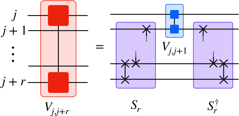
Figure 1: The quantum circuit for implementing an interaction between two qubits at distance $r$ on a superconducting quantum processor with only nearest-neighbor connectivity.

Superconducting quantum processors have a planar geometry and limited connectivity, and the only available connectivity of the IBM quantum processors at our disposal is nearest neighbors. However, the set of native gates that can be implemented on such devices is universal, meaning that every $N$-qubit unitary operator can be decomposed into a set of two and single-qubit operations [71].

We consider the unitary evolution operator generated by the interaction between a couple of qubits. When these qubits are nearest neighbors, say at sites $j$ and $j+1$ of the quantum processor and thus physically connected, this operator can be written simply in terms of the available operations resulting in the two-qubit unitary gate $V_{j,j+1}=V\otimes\mathbb{1}_{j+2,\dots,j+r}$. We consider the action of this gate on a generic state of the computational basis ${\left|\mathbf{s}\right\rangle=\left|s_{j},\dots,s_{j+r}\right\rangle}$, where $s_{j},\dots,s_{j+r}=0,1$. It can be written in general as

$$V_{j,j+1}\left|\mathbf{s}\right\rangle=\sum_{s_{a},s_{b}=0}^{1}c_{s_{a},s_{b}}\left|s_{a},s_{b}\dots,s_{j+r}\right\rangle,$$ (11)

where $c_{s_{a},s_{b}}=\left\langle s_{a},s_{b}\right|V\left|s_{j},s_{j+1}\right\rangle$. The result for a generic initial state will then simply follow by linearity. Our objective is to extend this operation to effectively implement the same interaction but between two qubits at distance $r$, say at sites $j$ and $j+r$, which are not physically connected on the hardware, i.e., the quantum gate $V_{j,j+r}$. This may be achieved through the quantum circuit in Fig. 1.

The idea is to exchange the qubit states by applying a sequence of SWAP gates (represented by crosses connected by a line in Fig. 1) among the couples of physically connected qubits that lie between $j$ and $j+r$. By doing so, the initial state of qubit $q_{j+r}$ is effectively encoded in qubit $q_{j+1}$. Specifically, we achieve this by applying the gate sequence:

$$S_{r}=\prod_{l=1}^{r-1}\mathrm{SWAP}_{j+l,j+l+1},$$ (12)

to the initial state $\left|\mathbf{s}\right\rangle$, resulting in:

$$S_{r}\left|s_{j},s_{j+1},\dots,s_{j+r}\right\rangle=\left|s_{j},s_{j+r},s_{j+1}\dots,s_{j+r-1}\right\rangle.$$ (13)

Next, we apply $V_{j,j+1}$ on the first two qubits, leading to:

$$V_{j,j+1}S_{r}\left|\mathbf{s}\right\rangle=\sum_{s_{a},s_{b}=0}^{1}c_{s_{a},s_{b}}\left|s_{a},s_{b},s_{j+1}\dots,s_{j+r-1}\right\rangle.$$ (14)

Finally, we need to bring back the state encoded in qubit $q_{j+1}$ to the $r$-neighbor qubit $q_{j+r}$. This is achieved by applying the inverse sequence of SWAP gates:

$$S_{r}^{\dagger}=\prod_{l=r-1}^{1}\mathrm{SWAP}_{j+l,j+l+1},$$ (15)

resulting in:

$$S_{r}^{\dagger}V_{j,j+1}S_{r}\left|\mathbf{s}\right\rangle =\sum_{s_{a},s_{b}=0}^{1}c_{s_{a},s_{b}}\left|s_{a},s_{j+1}\dots,s_{b}\right\rangle$$

$$=V_{j,j+r}\left|\mathbf{s}\right\rangle.$$ (16)

Here, we observe that the final result is the same as the one obtained by applying the $r$-range gate $\left|\mathbf{s}\right\rangle$ on the initial state. Since this equality holds for any state $\left|\mathbf{s}\right\rangle$ of the qubits’ computational basis, we can conclude that

$$V_{j,j+r}=S_{r}^{\dagger}V_{j,j+1}S_{r}.$$ (17)

Therefore, the quantum circuit in Fig. 1 is equivalent to the dynamics generated by the $r$-range interaction among the physically unconnected qubits $q_{j}$ and $q_{j+r}$. However, this comes at a cost: we need to apply $2(r-1)$ additional $\mathrm{SWAP}$ gates. Since every two-qubit gate typically introduces noise, we will need to mitigate effect of the noise as the interaction rate increases. We address this problem in the following sections.

Quantum circuit implementation of the Floquet dynamics

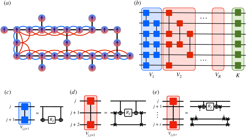
Figure 2: Quantum circuit implementation of Floquet dynamics with varying interaction range. (a) Topology of the ibmq_mumbai quantum processor. Black links represents the physical connections among the qubits on the quantum hardware, blue and red links represent the nearest neighbors $R=1$ and next to nearest neighbors $R=2$ Ising interaction we effectively implemented among physically unconnected qubits during our quantum simulation. (b) Quantum circuit implementing a single Floquet step for a kicked Ising model with $R$ range interactions. (c) Quantum gate implementation of nearest neighbor Ising interaction among qubit $j$ and $j+1$. (d) Quantum gate implementation of next to nearest neighbor Ising interaction among qubit $j$ and $j+2$. (e) Quantum gate implementation of $r$-neighbor Ising interaction among qubit $j$ and $j+r$.

To simulate the Floquet dynamics with varying interaction range on an IBM quantum processor, we transform the quantum evolution into a quantum circuit. We utilize the imbq-mumbai 27-qubit processor, whose topology is depicted in Fig. 2a (further technical details can be found in the Supplementary material). Our quantum circuit is optimized using the available connectivity and native gates of the device, including the controlled-not gate $\mathrm{CNOT}$, the identity gate $\mathrm{ID}$, rotations along the z-axis $RZ$, the NOT gate $X$, and the $\mathrm{SX}=\sqrt{X}$ gate. For more information on the decomposition of our quantum circuit into native gates and its optimization we refer the reader to the Methods section.

We begin by noting that the Floquet unitary evolution operator at stroboscopic times $t=nT$ can be obtained by applying the unitary operator corresponding to each Floquet step $U_{F}$ $n$ times, i.e., $U(nT)=(U_{F})^{n}$. Importantly, no Trotter approximation is required, which is a significant advantage of Floquet drivings, making them well-suited for quantum circuit implementation [2]. Furthermore, as shown in the introduction, the kicked Floquet protocol of interest can be further decomposed into the successive application of the kick operator $K_{\phi}$ and the Ising evolution operator $V$ (see Eq. (5)). The former can be expressed in terms of single-qubit gates, corresponding to local rotations along the x-axis, and the latter can be written as a product of mutually commuting unitaries that connect pairs of qubits at progressively larger distances as the interaction range is increased, i.e., $K_{\phi}=\prod_{i=1}^{N}R_{x,i}(2\phi)$ and $V=\prod_{r=1}^{R}V_{r}$, respectively. Each $V_{r}$ can be implemented by applying the general method to effectively realize $r$-range interactions introduced in the previous section.

The quantum circuit corresponding to a single Floquet step is shown in Fig. 2b, where blue gates represent nearest-neighbor Ising interactions $V_{j,j+1}$, red gates represent Ising interactions beyond nearest neighbors, $V_{j,j+r}$, and green gates represent the final kick rotation $K_{\phi}$ applied equally to each qubit. In particular, as shown in Fig. 2c, the unitary operator associated to nearest neighbors Ising interactions can be decomposed in terms of the elementary gates as

$$V_{j,j+1} =e^{iTJ_{1}Z_{j}Z_{j+1}}$$

$$=\mathrm{CNOT}_{j,j+1}R_{Z}(2J_{1}T)\mathrm{CNOT}_{j,j+1}.$$ (18)

On the other hand, the limited processor connectivity does not allow for a simple decomposition of $r$-range Ising interactions. As a consequence, we need to specify the general method introduced in the previous section obtaining the decomposition

$$V_{j,j+r}=S_{r}^{\dagger}\mathrm{CNOT}_{j,j+1}R_{Z}(2J_{1}T)\mathrm{CNOT}_{j,j+1}S_{r},$$ (19)

where $S_{r}$ is the sequence of $\mathrm{SWAP}$ gates defined in Eq. 12.

The Role of Noise and Noise Mitigation

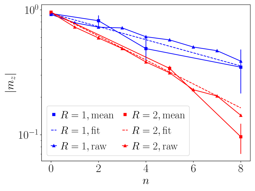
Figure 3: Modulus of the magnetization $|m_{z}|$ as a function of the stroboscopic times $n$ for nearest neighbors $R=1$ (blue points) and next to nearest neighbors $R=2$ (red points) Ising interactions. Triangles represent the raw experimental data measured on our quantum simulation of the ibmq_mumbai quantum processor which involves $N=18$ qubits undergoing a kicked Ising dynamics with kick angle $\phi=\pi/2+\epsilon$ with $\epsilon=0.2$. Square points and the corresponding error bars represent the estimators for the average magnetization and its statistical error $\mathbb{E}(m_{z})\pm 2\sigma(m_{z})$, obtained through statistical bootstrapping. Dashed lines represents the best fit of the data with an exponential decay.

The analysis of the raw experimental data clearly demonstrates that the decay of magnetization is predominantly influenced by the effect of noise, as illustrated in Figure 3. The figure depicts the absolute value of the average magnetization $|m_{z}|$ as a function of the stroboscopic time $n$ for nearest neighbors ($R=1$, in blue) and next-to-nearest neighbors ($R=2$) interactions. The raw experimental data (triangles in Fig. 3) are obtained by running $n$ repetitions of the quantum circuit corresponding to a single Floquet step $U_{F}$, as depicted in Fig. 2b, on the ibmq_mumbai quantum processor with $N=18$ qubits. At the end of each quantum evolution, a projective measurement of each qubit in the $Z$ basis is performed. To collect sufficient statistics, the experiments for each value of $n$ and $R$ are repeated over a sample of size $\mathcal{N}=2^{13}$, allowing us to compute the sample average $\langle Z_{i}\rangle$ over the measurement outcomes. Finally, the spatial average of the magnetization over different sites of the processor is computed as

$$m_{z}=\frac{1}{N}\sum_{i=1}^{N}\langle Z_{i}\rangle,$$ (20)

where $N=18$ in our case.

Estimating the statistical error from multiple instances of each quantum simulation to evaluate the sample mean $\mathbb{E}(m_{z})$ and standard deviation $\sigma(m_{z})$ is not feasible due to the time taken to produce each magnetization estimate. Instead, we rely on the statistical tool of bootstrapping, which is further detailed in the Methods section, to generate resampled data from the empirical measurement outcomes. Since the bootstrapped data conforms to the central limit theorem, we may assume normality and evaluate $\mathbb{E}(m_{z})$ and $\sigma(m_{z})$ from these artificially generated samples of data. The results for the statistical averages $\mathbb{E}(m_{z}(n))$ are represented by squares in Fig. 3, while we use two standard deviations, $2\sigma(m_{z}(n))$, as statistical errors, depicted as error bars in the plots. Notably, we observe that the statistical error increases with the number of Floquet steps involved in the dynamics $n$. This can be understood by a simple statistical argument: we are trying to sample a quantity, the modulus of the magnetization $|m_{z}|$, which exponentially decreases with $n$. Consequently, the resolution with which we can estimate this quantity deteriorates as $m_{z}$ approaches the value $m_{z}\sim e^{-\gamma n}\sim 1/\sqrt{\mathcal{N}}$, i.e., the statistical uncertainty due to the finite size of the sample increases as we approach the stroboscopic time $n\sim(1/2\gamma)\ln\mathcal{N}$.

The decay of magnetization with stroboscopic time $n$ can be described by an exponential fit $|\mathbb{E}(m_{z}(n))|=ae^{-bn}$, which is obtained using a weighted least squares regression method. This approach accounts for points with high statistical uncertainty, penalizing them in the extrapolation. The resulting exponential decay is depicted as a dashed line in Fig. 3, showing a rapid decline with increasing $n$. Notably, the decay rate is more pronounced for next-to-nearest neighbor interactions ($R=2$) compared to nearest neighbor interactions ($R=1$). This discrepancy can be attributed to the fact that the quantum circuit implementing next-to-nearest neighbor interactions involves more gates, resulting in larger noise effects.

In order to effectively simulate desired physical phenomena in a quantum system, it is crucial to account for and mitigate the detrimental effects of noise. Real-world quantum hardware is susceptible to various sources of errors, such as noisy gates, environmental decoherence, and spurious time dependence of circuit parameters [2]. To explicitly model these errors, a common approach is to consider one- and two-qubit depolarizing channels that act on the system’s state $\rho$. Specifically, after each single-qubit gate acting on qubit $i$, the single-qubit channel $\phi_{i}^{1q}$ is applied, while after each two-qubit gate on bond $(i,j)$, the two-qubit channel $\phi_{i,j}^{2q}$ is applied. These channels are defined as [71, 2]

$$\phi_{i}^{1q}(\rho) =(1-p_{1})\rho+\frac{p_{1}}{3}(X_{i}\rho X_{i}+Y_{i}\rho Y_{i}+Z_{i}\rho Z_{i})$$ (21)

$$\phi_{i,j}^{2q}(\rho) =(1-p_{2})\rho+\frac{p_{2}}{15}\sum_{\alpha,\beta=1}^{3}(\sigma_{\alpha,i}\sigma_{\beta,j}\rho\sigma_{\alpha,i}\sigma_{\alpha,j}),$$ (22)

where $X_{i}$, $Y_{i}$, and $Z_{i}$ are the Pauli matrices for qubit $i$, and $\sigma_{\alpha,i}$ and $\sigma_{\beta,j}$ are the corresponding matrices for qubits $i$ and $j$, respectively. By studying the dynamics of the $Z_{i}$ operators under these depolarizing channels, we can estimate the magnetization decay rate induced by the noisy gates.

To isolate the effect of noise, we consider the case of perfect kick dynamics with $\epsilon=0$. Under this condition, $Z_{i}$ is invariant under the two-qubit Ising interaction gates and simply acquires a minus sign under the $\pi$ rotation around the x-axis. However, after each two-qubit gate, $Z_{i}$ decays under $\phi_{i,j}^{2q}$ as

$$\phi_{i,j}^{2q}(Z_{i})=(1-16p_{2}/15)Z_{i},$$ (23)

and after each single-qubit gate as

$$\phi_{i}^{1q}(Z_{i})=(1-4p_{1}/3)Z_{i}.$$ (24)

Overall, $Z_{i}$ decays to $-e^{-\gamma_{\mathrm{dep}}}Z_{i}$, over one noisy Floquet step with perfect kicks, with $\gamma_{\mathrm{dep}}$ given by

$$\gamma_{\mathrm{dep},R}=-\ln[(1-16p_{2}/15)^{\mathcal{Q}_{2q,R}}(1-4p_{1}/3)^{\mathcal{Q}_{1q,R}}],$$ (25)

where $\mathcal{Q}_{2q,R}$ and $\mathcal{Q}_{1q,R}$ are the number of two-qubit and single-qubit gates involved in a Floquet step quantum circuit with $R$-neighbors interactions. A naive estimate of these numbers based on the general method previously introduced would yield $\mathcal{Q}_{2q,R}=2R^{3}+2$ and $\mathcal{Q}_{1q,R}=2R+5$, respectively (see Methods for more details). However, for the specific case of the Kicked Ising model considered in our quantum simulations, we were able to optimize the quantum circuits corresponding to $R=1,2$ Floquet steps, reducing the number of two qubits native gates, involved in the quantum circuit longest path, to $\mathcal{Q}_{2q,R}=9R^{2}-14R+7$, with a reduction from cubic to quadratic range dependence. In particular for $R=1,2$ we have

$$\mathcal{Q}_{2q,R}=\begin{cases}4&R=1\\ 15&R=2\end{cases},\quad\mathcal{Q}_{1q,R}=\begin{cases}7&R=1\\ 9&R=2\end{cases}.$$ (26)

More details on the quantum circuit optimization strategy are provided in the Methods section.

Another source of noise arises from the finite decoherence time $T_{1}$ of the qubits, which introduces an additional time scale contributing to the magnetization decay. Taking into account all the contributions, we can estimate the decay rate of magnetization for a Floquet step with imperfect kicks of an angle $\phi=\pi/2+\epsilon$ to be approximately given by

$$\Gamma_{1,R}\approx\gamma_{\mathrm{dep},R}+\tau_{R}/T_{1}+\gamma_{\epsilon,R},$$ (27)

where $\tau_{R}$ represents the time required to practically implement the Floquet step on the quantum hardware. This can be estimated as

$$\tau_{R}=\mathcal{Q}_{1q,R}\tau_{1q}+\mathcal{Q}_{2q,R}\tau_{2q}+\tau_{m},$$ (28)

where $\tau_{1q}$ and $\tau_{2q}$ denote the time needed to execute each single-qubit and two-qubit gate, respectively, while $\tau_{m}$ represents the readout time required for measurements. Estimates of these quantities, as obtained from the engine calibration, are provided in the Supplementary material.

A third source of errors arises from readout errors, which can be modeled as a stochastic process where the outcome of a qubit state measurement (in the $Z$ computational basis) is randomly flipped with a probability of $p_{m}$ away from its correct value [2]. Specifically, if we define the probability that qubit $i$ points up (down) at time $n$ as $\Pi_{\pm}=\langle(1\pm Z_{i}(n))/2\rangle$, then the result of the noisy measurement process is $Z_{i}=\pm 1$ with a probability of $\tilde{\Pi}{\pm}^{(n)}=\Pi{\pm}(1-p_{m})+\Pi_{\mp}p_{m}$. Accordingly, the estimate for the expectation value of $Z_{i}$ becomes

$$\tilde{\Pi}_{+}-\tilde{\Pi}_{-} =(1-2p_{m})(\Pi_{+}-\Pi_{-})$$

$$=(1-2p_{m})\langle Z_{i}(n)\rangle.$$ (29)

Hence, averaging over positions yields $\tilde{m}_{z}=(1-2p_{m})m_{z}$, i.e., a damping by a time-independent and range-independent overall prefactor $C_{m}=(1-2p_{m})$.

The inclusion of noise in our model provides a compelling explanation for the rapid exponential decay of magnetization, as observed in Fig. 3. Moreover, by inserting the estimated values of the parameters $p_{1}$, $p_{2}$, $\tau$, and $T_{1}$, which were extracted from the calibration data provided by IBM and detailed in the Supplementary Materials, we find that the calculated decay rate is in good agreement with the one obtained from fitting the experimental data with a stroboscopic time dependence of the form predicted by our theoretical model

$$|m_{z}(n)|=C_{m}e^{-n\Gamma_{1,R}}$$ (30)

This understanding of the noise effect justifies our exploration of the possibility of mitigating it through a technique called zero noise extrapolation.

The basic idea of zero noise extrapolation is to intentionally increase the noise level by amplifying the depth of the quantum circuits by a factor of $s$ through a procedure called circuit folding (see Methods section for a detailed description). Subsequently, we perform quantum simulations for different noise scales, $s$, and for each scale, we extract the magnetization decay rate from the measured data. Our noise model then allows us to theoretically estimate the decay rate at noise scale $s$ as

$$\Gamma_{s,R}\approx s(\gamma_{\mathrm{dep},R}+\tau_{R}/T_{1})+\gamma_{\epsilon,R}.$$ (31)

Accordingly, a linear fit of the measured decay rates with respect to the parameter $s$ enables us to separate the contribution coming from the noise, $\gamma_{\mathrm{noise}}=\gamma_{\mathrm{dep},R}+\tau_{R}/T_{1}$, from $\gamma_{\epsilon,R}$, which represents the decay rate due to the internal system thermalization that destroys the time crystalline order at finite $\epsilon$, and should be stabilized by the presence of longer-range interactions. More precisely, $\gamma_{\epsilon,R}$ is obtained as the zero noise extrapolation of the decay rate in Eq. (31)

$$\gamma_{\epsilon,R}\approx\Gamma_{s=0,R}.$$ (32)

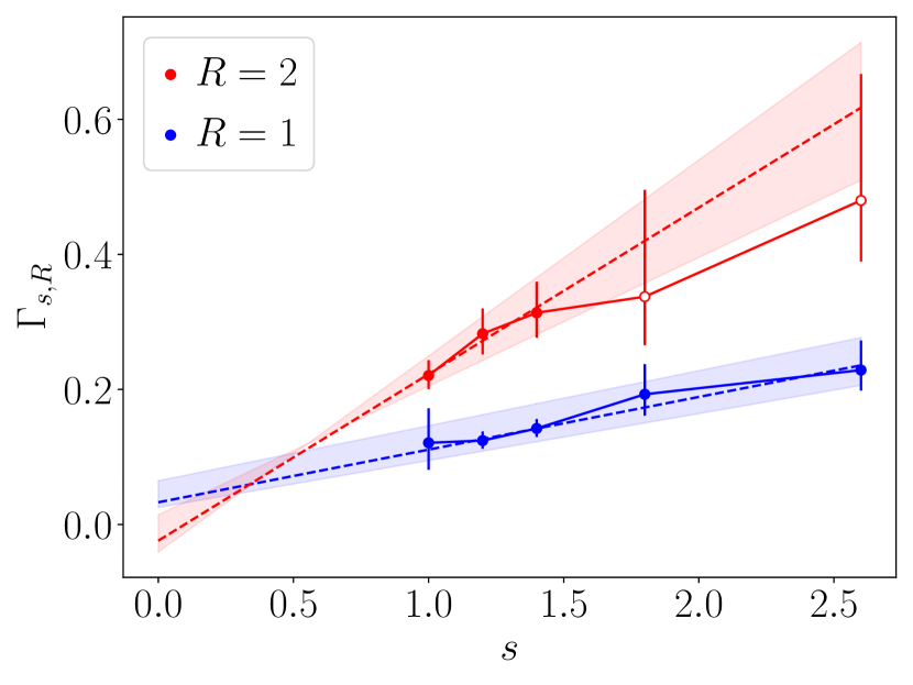
Figure 4: Decay rate of magnetization as a function of noise scale $s$ for $R=1$ (blue points) and $R=2$ (red points). Error bars represent two standard deviations $\sigma(m_{z})$ estimated through statistical bootstrapping. Dashed lines indicate the best linear fit obtained using weighted least squares regression. Empty points are excluded from the fitting data.

The results of this procedure are shown in Fig. 4, where the measured decay rate is plotted as a function of the noise scale $s$. To estimate $\Gamma_{s,R}$ and its uncertainty $\delta\Gamma_{s,R}$, we first estimate the magnetization as a function of the stroboscopic time $n$ at different values of $s$ and $R$ from the measured data, along with the corresponding statistical uncertainty from the standard deviation obtained through the statistical bootstrap method, $\mathbb{E}(m_{z})\pm 2\sigma(m_{z})$. Then, the decay rate and its uncertainty are obtained through the exponential fit

$$|\mathbb{E}(m_{z})\pm 2\sigma(m_{z})|=(C_{m}\pm\delta C_{m})e^{-n(\Gamma_{s,R}\pm\delta\Gamma_{s,R})}.$$ (33)

In particular, the exponential fit is performed using weighted least squares regression, and the last two points with $R=2$ and $s>1.5$ are excluded from the fitting data (empty points in Fig. 4). This exclusion is justified by the fact that the decay rate for these points falls within the range of $0.2<\Gamma_{s>1.5,2}<0.8$, and thus, the magnetization can be reliably estimated only for stroboscopic times $n<n^{*}\approx(1/2\gamma)\ln\mathcal{N}$, where $6<n^{*}<22$. Therefore, not all the time steps $1<n<16$ considered in the exponential fit of $m_{z}(n)$ from which we extracted this decay rate are within the reach of our statistical resolution. The difficulty of establishing a reliable bootstrap-estimated value confirms this phenomenon, as shown in Fig. 4, where the statistical error bars for these points are significantly larger than those for the other points, indicating the challenge of obtaining a trustworthy value for the magnetization in this regime. Despite the failure of the bootstrap procedure, we include these data as empty points in the plot for completeness, noting that the corresponding error bars are sufficiently large that the resulting fit is still compatible with these unreliable values within $\pm 2\sigma(m_{z})$.

Remarkably, upon extrapolation to the zero noise limit, the decay rate of the $R=2$ case is found to be smaller than that in the nearest neighbors case $R=1$. Specifically, we obtain

$$\Gamma_{0,2}\pm\delta\Gamma_{0,2}<\Gamma_{0,1}\pm\delta\Gamma_{0,1},$$ (34)

indicating that the extrapolated decay rate is consistent with the theoretical expectations within the statistical uncertainty $\delta\Gamma_{0,R}$, which has been estimated by extrapolating $\delta\Gamma_{s,R}$ to $s=0$.

Final results

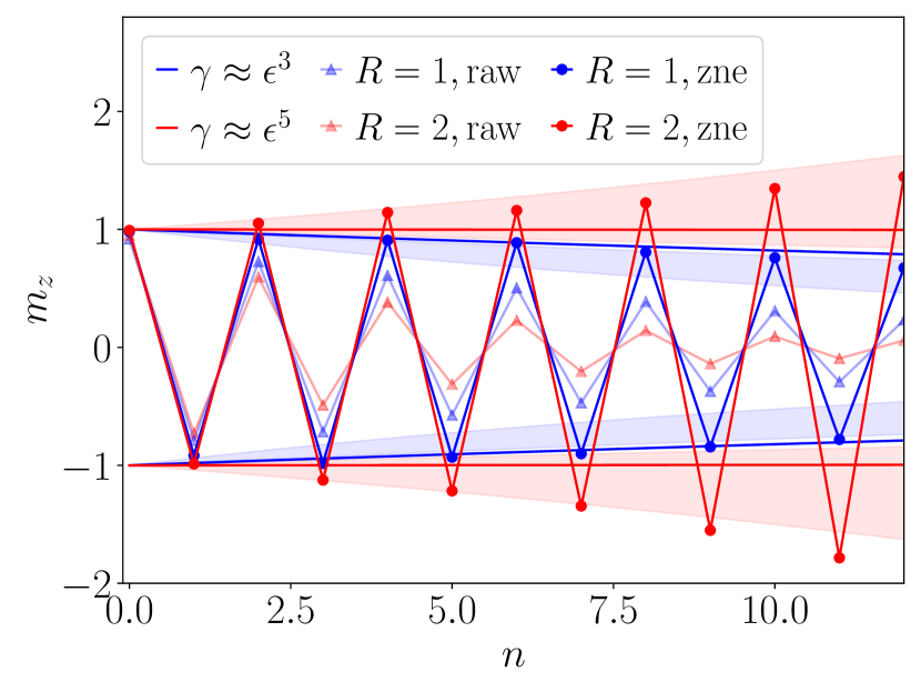
Figure 5: Magnetization $m_{z}$ as a function of stroboscopic times for nearest neighbors $R=1$ and next to nearest neighbors $R=2$ Ising interactions and kicks of an angle $\phi=\pi/2+\epsilon$, with $\epsilon=0.2$. Triangles represent the raw data with no noise mitigation, and full dots represent the mitigated data after zero noise extrapolation. The shaded red and blue areas represent the statistical uncertainty for $R=1$ and $R=2$ respectively. The dot-dashed lines represent the curves $\pm e^{-n\gamma_{\epsilon,R}}$, where $\gamma_{\epsilon,R}$ is the magnetization decay rate predicted from the theoretical model.

In this section we summarize the final results of our quantum simulation for the magnetization dynamics under a kicked Floquet driving. The zero noise extrapolation procedure allowed us to detect the role of noise and to separate it from the true decay caused by the dynamical generation of excitations in the system during the Floquet driving. Figure 5 shows the magnetization $m_{z}$ as a function of stroboscopic times for nearest neighbors $R=1$ and next to nearest neighbors $R=2$ Ising interactions and kicks of an angle $\phi=\pi/2+\epsilon$, with $\epsilon=0.2$. In particular triangles represent the raw data with no noise mitigation. As previously discussed, these points display a fast exponential decay dominated by noise with a faster decay rate for larger interaction range. This fact follows from the increased quantum circuit depth induced by next-to-nearest couplings, see Figure 2, which enhances the detrimental effects of noise. The result obtained after noise mitigation by zero noise extrapolation are displayed by full circles. More precisely, these points are obtained by multiplying the raw measured data for $m_{z}(n)$ by a factor $e^{(\Gamma_{s=1,R}-\Gamma_{s=0,R})n}/C_{m}=e^{\gamma_{\mathrm{noise}}n}$, so that the decay rate induced by noise $\gamma_{\mathrm{noise}}$ is removed and we are only left with the desired decay rate $\gamma_{\epsilon,R}=\Gamma_{0,R}$. The shaded red and blue areas represent the statistical uncertainty, for $R=1$ and $R=2$ respectively. These have been estimated as the regions between $e^{-\Gamma_{0,R}\pm\delta\Gamma_{0,R}}$, where $\delta\Gamma_{0,R}$ is the decay rate uncertainty extrapolated to the zero noise limit. As expected from the statistical arguments previously introduced, the uncertainty grows with time. However, we notice that the two regions corresponding to the $R=2$ and $R=1$ zero noise extrapolated values of the magnetization never intersect within the considered stroboscopic time interval. Moreover, the decay in the nearest neighbor case is always faster with respect to that in presence of next to nearest neighbors interactions, in good agreement with theoretical expectations. Most significantly the magnetization decay rate analytically predicted from the theoretical model, $\gamma_{\epsilon,R}\approx\epsilon^{2R+1}$, is compatible with the final results of our quantum simulation within the estimated uncertainty. This is shown in Fig. 5 where the curves $\pm e^{-n\gamma_{\epsilon,R}}$, represented as solid lines, always lie within the shaded areas representing the values of $m_{z}(n)$ extracted from our quantum simulation.

Discussion

In this paper, we have demonstrated the potential of superconducting quantum hardware for advancing the field of digital quantum simulation by investigating the possibility of implementing quantum dynamics of systems with couplings beyond nearest neighbors. We have utilized the universality of the native gates in quantum processors to implement couplings among physically disconnected qubits, and carefully mitigated the effects of gate noise, measurement errors, and statistical errors from the raw results. Our focus has been on the stabilization of discrete Floquet time crystalline response as the interaction range increases, and we have implemented, on IBM quantum superconducting processors, a quantum simulation of a Floquet driven quantum spin chain with interactions beyond nearest neighbors.

Our results, as shown in Figure 5, reveal that the magnetization dynamics under a kicked Floquet driving exhibits a fast exponential decay dominated by noise in the raw data, with a faster decay rate for larger interaction ranges due to the increased depth of the quantum circuit. However, after applying the zero noise extrapolation procedure, we were able to separate the role of noise from the true decay caused by the dynamical generation of excitations in the system during the Floquet driving. The mitigated data, represented by the full dots in Figure 5, show a clear trend of slower decay compared to the raw data, indicating the effectiveness of our error mitigation approach.

Furthermore, we have estimated the statistical uncertainty of the mitigated data, represented by the shaded red and blue areas in Figure 5, which grows with time as expected. Importantly, we have observed that the regions corresponding to the zero noise extrapolated values of the magnetization for different interaction ranges do not intersect within the considered stroboscopic time interval, indicating that the effects of noise have been effectively removed from the data.

We have also compared our results with the theoretical expectations, and found that the magnetization decay rate analytically predicted from the theoretical model, $\gamma_{\epsilon,R}\approx\epsilon^{2R+1}$, is compatible with the final results of our quantum simulation within the estimated uncertainty. This agreement between theory and experiment provides evidence for the validity of our approach in simulating quantum systems with interaction ranges beyond the limits imposed by hardware connectivity.

It is important to highlight that the proposed method for implementing beyond nearest-neighbor interactions on quantum superconducting computers has the potential to enable tunable interaction ranges. However, there is a fundamental limitation that led us to restrict our quantum simulations to cases where $R=1,2$. This is due to the fact that increasing the effective range of interaction will inevitably require a deeper quantum circuit, which in turn increases the impact of noise. Practically speaking, we anticipate that already at $R=3,4$, the noise level may be significant enough to prevent a reliable estimate of the magnetization decay.

Nevertheless, there are several steps that can be taken to overcome this problem. For example, the noise level of quantum devices is expected to decrease as the performance of available quantum computers improves. Additionally, classical algorithms can be used to further optimize the quantum circuit we proposed, reducing the number of two-qubit gates involved. Furthermore, it would be instructive to benchmark our results on different experimental platforms that naturally allow for the implementation of long-range interactions, such as trapped ions or Rydberg atoms devices. These exciting problems are beyond the scope of the present work, hence we leave them for future research.

Another crucial aspect to emphasize is that in our quantum simulation, we utilize 18 functional qubits out of the total 27 nominal qubits of the ibmq_mumbai device. This distinction is significant since the number of functional qubits is often smaller in other applications. For instance, in quantum chemistry applications, as described in Ref. [72], noise mitigation strategies are employed to simulate molecules whose Hamiltonian can be encoded in only three qubits in order to achieve the desired chemical accuracy. This exemplifies the suitability of Floquet dynamics, similar to the ones analyzed in our work, for implementation on NISQ quantum computers.

In conclusion, our quantum simulation on IBM quantum superconducting processors has demonstrated the potential of these platforms for simulating quantum systems with couplings beyond nearest neighbors, and has offered insights into the fundamental physics of long-range systems. Our error mitigation approach has been effective in removing the effects of noise and measurement errors from the raw results, and the mitigated data are in good agreement with theoretical expectations. This work opens up new possibilities for studying quantum systems with long-range interactions and paves the way for further advancements in the field of digital quantum simulation on superconducting quantum hardware.

Methods

.2 Quantum circuit optimization

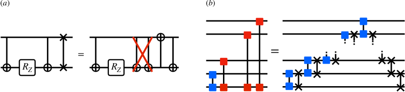
Figure 6: Quantum circuit optimization techniques using circuit identities. (a) Cancellation of $\mathrm{CNOT}$ gates in adjacent $V_{j,j+1}$ and $\mathrm{SWAP}$ gates. (b) Rearrangement of the quantum circuit to implement Ising interactions with $r=1,\dots,R$ ranges while maximizing the number of adjacent $V_{j,j+1}$ and $\mathrm{SWAP}$ gates.

As discussed in the Results section, minimizing the number of operations in the quantum circuit for implementing the Floquet dynamics is crucial due to the increase in noise with each quantum gate, resulting in a rapid magnetization decay. In particular, two-qubit gates are more prone to errors, so our focus is on reducing their number in our circuits.

We start by obtaining an estimate of the number of operations required to implement the quantum circuit shown in Fig. 2b using the native gates of the ibmq_mumbai processor used in this work, without any optimization. The native gates include the controlled-not gate ($\mathrm{CNOT}$), identity gate ($\mathrm{ID}$), rotations along the z-axis ($R_{Z}$), the NOT gate ($X$), and the $\mathrm{SX}=\sqrt{X}$ gate.

Regarding single-qubit gates, only the rotations around the $X$ axis, corresponding to the Floquet driving kicks, need to be further decomposed into native gates, which can be efficiently done as follows

$$R_{X}(\phi)=R_{Z}(\pi/2)\sqrt{X}R_{Z}(\phi)\sqrt{X}R_{Z}(5\pi/2).$$ (35)

Thus, each kick requires five additional single-qubit gates, resulting in a total of $Q_{1q,R}=2R+5$ gates. The only native two-qubit gate available is the $\mathrm{CNOT}$ gate. To estimate $Q_{2q,R}$, we need to count the number of $\mathrm{CNOT}$ gates involved in the hardware implementation of each Floquet step. As shown in Fig. 2c, each nearest-neighbor Ising interaction is implemented using two $\mathrm{CNOT}$ gates. Moreover, each $\mathrm{SWAP}$ gate is realized using three $\mathrm{CNOT}$ gates, as it can be decomposed as

$$\mathrm{SWAP}_{j,j+1}=\mathrm{CNOT}_{j,j+1}\mathrm{CNOT}_{j+1,j}\mathrm{CNOT}_{j,j+1}.$$ (36)

Moreover, each $r$-range interaction is implemented by adding $2(r-1)$ $\mathrm{SWAP}$ gates to the nearest-neighbor interaction. Therefore, each $r$-range interaction gate requires $2+6(r-1)$ $\mathrm{CNOT}$ gates for implementation. If we want to realize interactions with ranges $r=1,\ldots,R$, then the longest path, determining the circuit depth, contains $r$ non-parallelizable copies of each $r$-range operation for $r>1$ and two copies for $r=1$. Summing up all the contributions, we obtain:

$$Q_{2q,R}=\sum_{r>1}^{R}(2+6r(r-1))+4=2R^{3}+2.$$ (37)

We can optimize the structure of our quantum circuit (Figure 2b) to reduce its depth and complexity. First of all, we notice that, as shown in Fig. 6a, each time we have a sequence $V_{j,j+1}\mathrm{SWAP}{j,j+l}$, we can use the fact that $\mathrm{CNOT}^{2}=\mathbb{1}$ to eliminate two adjacent $\mathrm{CNOT}$ gates. To systematically exploit this fact, we can rearrange our quantum circuit using the circuit identity in Fig. 6b. Here, we utilize the properties $[V_{j,j+l},V_{j,j+r}]=0$ for all $l,r$, and $[V_{j,j+1},\mathrm{SWAP}_{j,j+l}]=0$ to maximize the number of adjacent $V_{j,j+1}\mathrm{SWAP}_{j,j+l}$, and thereby increase the number of $\mathrm{CNOT}$ gates that cancel out. for a circuit implementing a sequence of Ising interactions of ranges $r=1,\dots R$, we can cancel up to $2(R-1)$ $\mathrm{CNOT}$ gates using this trick. The depth of each subcircuit of this form is then given by

$$2R+6(R-1)-2(R-1)=6R-4.$$ (38)

To realize a kicked Ising model with interaction range up to $R$ in a chain of $N$ qubits, we can divide the $N$ qubits into subsets of size $2R$ that can be processed in parallel. To compute the circuit depth, which refers to the number of operations in the longest path, we can focus on only one subset at a time. Each subset contains $R$ subcircuits with interaction ranges $r=1,\ldots,R$, following the form shown in Fig. 6b. The depth of each of these subcircuits is $6R-4$. The remaining $R$ subcircuits include interactions of range $r=1,\ldots,l$, where $l$ varies from $l=1$ to $l=R-1$, corresponding to a depth of $6l-4$ for each circuit. By summing up all the contributions, we obtain the optimized number of $\mathrm{CNOT}$ gates as:

$$Q_{2q,R} =R(6R-4)+\sum_{l=1}^{R-1}(6l-4)$$

$$=9R^{2}-11R+4.$$ (39)

Finally, we observe that the last sequence of $\mathrm{SWAP}$ gates in the circuit shown in Fig. 6b is only necessary if we need to apply different gates on different qubits after that. If this is not the case, we can simply substitute the $\mathrm{SWAP}$ gates with a relabeling of the qubit numbers, which must be taken into account when reading the final measurement outcomes. This fact allows us to eliminate $(R-1)$ $\mathrm{SWAP}$ gates and $3(R-1)$ $\mathrm{CNOT}$ gates in the last subcircuit of this form. Therefore, we obtain:

$$Q_{2q,R}=9R^{2}-14R+7.$$ (40)

As a final remark, we note that for large values of maximum range $R$, and hence large circuit complexity, additional simplifications of the circuit may be possible by using optimized relabelings of the qubit numbers during the evolution, which can increase the number of parallelizable operations. However, such optimization strategy is circuit and range dependent, and can only be carried out numerically or in an approximate manner. On the other hand, for the case of $R=2$ that we considered in our quantum simulation, we can claim that our circuit is optimal with respect to the number of $\mathrm{CNOT}$ gates involved.

Circuit folding and Zero noise extrapolation

Zero noise extrapolation (ZNE) is a well-studied error mitigation method in the literature [73, 74, 75, 72]. It is a powerful technique that allows for the estimation of noiseless expectation values of observables from a series of measurements obtained at different levels of noise. The ZNE process involves two steps: intentional scaling of noise and extrapolation to the noiseless limit. In the first step, the target circuit is executed at varying error rates denoted by $s$, with expectation values estimated for the original circuit ($s=1$) as well as circuits at increased error rates ($s>1$). Then, in the second step, a function, motivated by physical arguments, is fitted to these expectation values and used to extrapolate to error rate $s=0$, providing an error-mitigated estimate.

There are various methods to increase the error rate $s$. Examples in the literature include pulse stretching [74] or, at a gate-level, unitary folding [73, 76]. In our implementation of ZNE, we increase $s$ using a local unitary folding technique. This technique involves increasing the number of operations by applying a mapping $U\to UU^{\dagger}U$ to individual gates of the circuit. Specifically, the unitary gates to be folded are randomly chosen from the set of gates composing the circuit, in such a way that the circuit depth is approximately increased by the desired factor $s$. This random selection helps to ensure that the circuit is exposed to a variety of gate sequences and interactions, allowing for a more comprehensive study of the circuit’s behavior under different noise conditions.

Statistical Bootstrapping

We utilize the statistical technique of bootstrapping to quantify the uncertainty in our magnetization estimates.In an ideal scenario, we would repeat quantum experiments multiple times to obtain a comprehensive understanding of the ’true’ magnetization distribution. However, this approach is impractical due to the significant time required for each magnetization estimate. Instead, we conduct the experiment once and generate resampled measurement data from the empirical distribution using bootstrapping, a widely used statistical technique. This method makes the statistical analysis very convenient and it is then becoming a common practice to estimate the statistical errors in digital quantum simulations [72].

Let us assume we perform an $\mathcal{N}$-shot quantum experiment and obtain a collection of $\mathcal{N}$ outcomes. Each measurement outcome is represented as a string of 0s and 1s, denoted as $Z_{1,a}\dots Z_{N,a}$, where $Z_{i}=0,1$, $N$ is the number of measured qubits, and the index $a$ labels the different outcomes ($a=1,\dots,\mathcal{N}$).The magnetization associated with each string can be computed by averaging over the qubits as follows

$$m_{z,a}=\frac{1}{N}\sum_{i=1}^{N}Z_{i,a}.$$ (41)

This gives us the set of magnetization values ${m_{z,a}}$ with $a=1,\dots,\mathcal{N}$. We define the empirical magnetization distribution $P_{1}(m_{z,a})$ as the histogram of the ${m_{z,a}}$ set. he average over this empirical distribution, denoted as $m_{z}$, corresponds to the experimentally obtained quantum expectation value on the final state of the system and can be expressed as

$$m_{z}=\frac{1}{N}\sum_{i=1}^{N}\langle Z_{i}\rangle=\sum_{a=1}^{\mathcal{N}}P_{1}(m_{z,a})m_{z,a}.$$ (42)

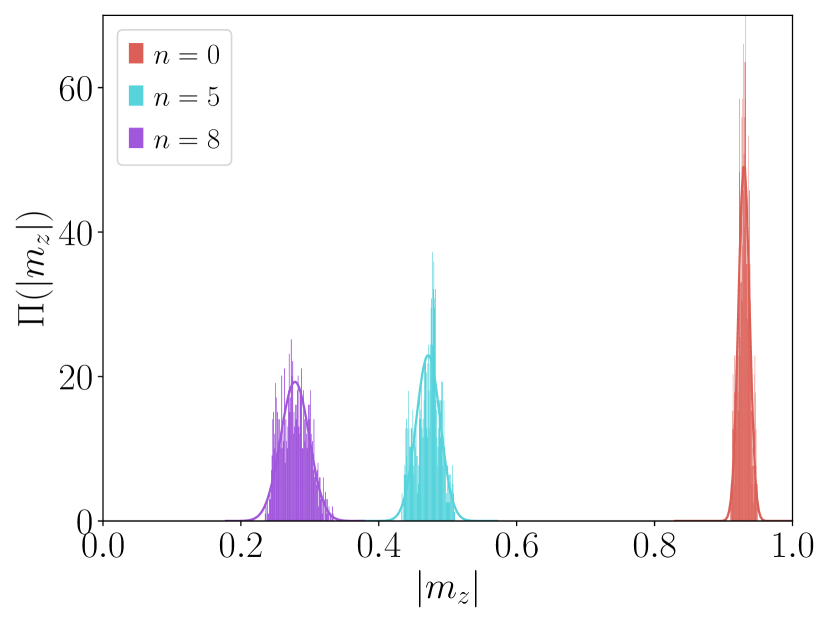
Figure 7: Bootstrap distribution of averages obtained by resampling $M=1000$ times the measured data of three quantum simulations with range $R=1$, noise scale $s=1.4$ and different numbers of Floquet steps $n=0,5,8$. The number of bins considered in each histogram is $100$.

The bootstrapping approach involves resampling from the empirical measurement distribution $P_{1}(m_{z,a})$. We sample elements from the set ${m_{z,a}}$ (or equivalently from the set of strings $\{Z_{1,a}\dots Z_{N,a}\}$) $\mathcal{N}$ times to create a new set of measurement outcomes, and from this, a new empirical distribution $P_{2}(m_{z,a})$.We repeat this process as many times as possible given the available computational resources, say $M$ repetitions, to obtain a set of distributions ${P_{1},P_{2},\dots,P_{M}}$. From each of these distributions, we can compute the average $m_{z}^{\alpha}$ with $\alpha=1,\dots,M$, and from the histogram of the set of averages, we obtain their distribution $\Pi(m_{z}^{\alpha})$.Since each resampling is independent, the distribution of averages should tend to a Gaussian in the large $M$ limit, according to the central limit theorem. Accordingly, we can define our estimator for $m_{z}$ and its statistical error as the average of the $\Pi(m_{z}^{\alpha})$ distribution

$$\mathbb{E}(m_{z})=\sum_{\alpha=1}^{M}\Pi(m_{z}^{\alpha})m_{z}^{\alpha},$$ (43)

and its standard deviation

$$\sigma(m_{z})=\sqrt{\sum_{\alpha=1}^{M}\Pi(m_{z}^{\alpha})(m_{z}^{\alpha}-\mathbb{E}(m_{z}))^{2}}.$$ (44)

This method enables us to obtain error bars in Figs 3 and 4 as $\mathbb{E}(m_{z})\pm 2\sigma(m_{z})$. Figure 7 shows, as an example, the distributions $\Pi(m_{z}^{\alpha})$ obtained through $M=1000$ resamples of the measured data of three quantum simulations with range $R=1$, noise scale $s=1.4$, and number of Floquet steps $n=0,5,8$, respectively. These are compared with Gaussian distributions with the same mean and standard deviation, finding good agreement. We notice that, as expected, the mean $\mathcal{E}(m_{z})$ is smaller for a larger number of Floquet steps $n$, signaling the magnetization exponential decay. Moreover, distributions at later stroboscopic times become broader, signaling the growth of the statistical error due to the fact that we are trying to sample a quantity which is exponentially decaying with $n$. For the sake of completeness, the full dataset obtained from the statistical bootstrap method applied to the quantum simulation considered in this study is provided in the Supplementary Materials.

Appendix A Calibration details of the quantum processor

In this section, we provide all the calibration details of the ibmq_mumbai backend, which is one of the 27-qubit IBM Falcon processors used in our experiments. Figure S.1 shows the topology of the processor and the qubit labeling numbers. We present the corresponding coupling map for two-qubit gates in Figure S.2, which includes the $\mathrm{CNOT}$ gate error $p_{2}$ (panel a) and the $\mathrm{CNOT}$ gate length $\tau_{2q}$ (panel b) for each pair of physically connected qubits on the device. Table S.1 reports the following properties for each qubit of the processor: relaxation time $T_{1}$, decoherence time $T_{2}$, single-qubit gate length $\tau_{1q}$, single-qubit gate error $p_{1}$, readout length $\tau_{m}$, and readout error $p_{m}$.

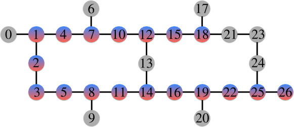
Figure S.1: Topology of the ibmq_mumbai quantum processor with numbered qubits. Grey qubits were not involved in our quantum simulations.

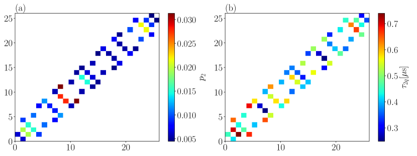
Figure S.2: Coupling map and calibration data for the $\mathrm{CNOT}$ gates of ibmq_mumbai quantum processor at the time our experiments were performed. (a) $\mathrm{CNOT}$ error. (b) $\mathrm{CNOT}$ lenght.

Qubit	$T_{1}[\mu\mathrm{s}]$	$T_{2}[\mu\mathrm{s}]$	$\tau_{1q}[\mathrm{ns}]$	$p_{1}\times 10^{4}$	$\tau_{m}[\mu\mathrm{s}]$	$p_{m}\times 10^{2}$
$q_{1}$	139.25	84.63	35.56	2.23	3.55	0.69
$q_{2}$	79.93	95.46	35.56	8.14	3.55	9.65
$q_{3}$	129.79	269.09	35.56	2.02	3.55	2.19
$q_{4}$	108.52	35.25	35.56	2.24	3.55	1.77
$q_{5}$	96.90	144.35	35.56	1.99	3.55	1.20
$q_{7}$	104.21	87.53	35.56	1.75	3.55	1.60
$q_{8}$	122.01	58.38	35.56	3.60	3.55	3.69
$q_{10}$	140.58	174.33	35.56	1.98	3.55	2.25
$q_{11}$	217.71	74.63	35.56	2.04	3.55	2.62
$q_{12}$	216.04	310.34	35.56	1.68	3.55	3.73
$q_{14}$	162.60	244.97	35.56	1.88	3.55	1.48
$q_{15}$	70.33	159.80	35.56	1.92	3.55	2.44
$q_{16}$	100.41	136.65	35.56	1.85	3.55	2.61
$q_{18}$	55.97	298.32	35.56	1.84	3.55	5.66
$q_{19}$	164.04	163.14	35.56	1.75	3.55	1.36
$q_{22}$	146.29	97.10	35.56	1.87	3.55	1.31
$q_{25}$	185.26	64.45	35.56	1.88	3.55	1.67
$q_{26}$	67.10	115.73	35.56	2.40	3.55	1.82

Table S.1: Calibration data for each qubit of the processor of the ibmq_mumbai quantum processor at the time our experiments were performed.

Appendix B Statistical bootstrap data

In this section we provide the complete dataset produced by applying the bootstrap procedure to the measured outputs of each quantum simulation performed on the ibmq_mumbai processor. In particular Fig. S.3 shows the bootstrap data for nearest neighbor Ising interactions $R=1$, different noise scales $s=1,1.2,1.4,2.6$ and different stroboscopic times $n=0,5,8,10,12$, while Fig. S.4 shows the same the bootstrap data for next to nearest neighbor Ising interactions $R=2$, different noise scales $s=1,1.2,1.4,2.6$ and different stroboscopic times $n=0,5,8$.

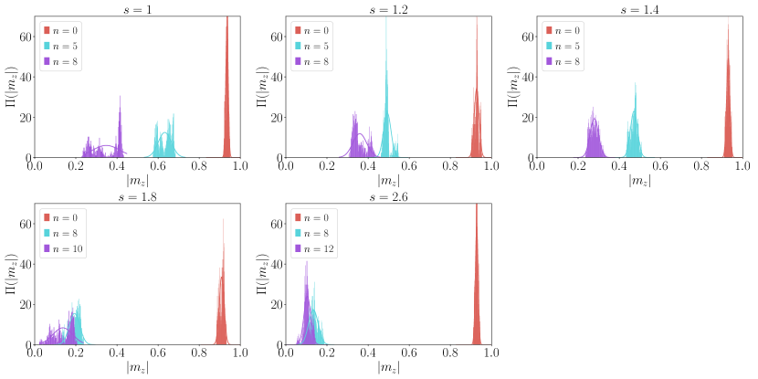
Figure S.3: Bootstrap distribution of averages obtained by resampling $M=1000$ times the measured data of the quantum simulations with range $R=1$, noise scales $s=1,1.2,1.4,1.8,2.6$ and different numbers of Floquet steps $n=0,5,8,10,12$. The number of bins considered in each histogram is $100$.

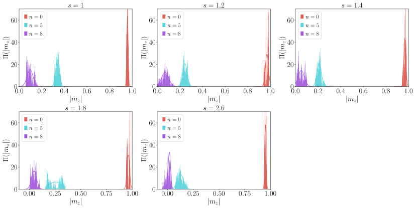
Figure S.4: Bootstrap distribution of averages obtained by resampling $M=1000$ times the measured data of the quantum simulations with range $R=2$, noise scales $s=1,1.2,1.4,1.8,2.6$ and different numbers of Floquet steps $n=0,5,8$. The number of bins considered in each histogram is $100$.

References

- Preskill [2018] J. Preskill, Quantum Computing in the NISQ era and beyond, Quantum 2, 79 (2018).
- Ippoliti et al. [2021] M. Ippoliti, K. Kechedzhi, R. Moessner, S. Sondhi, and V. Khemani, Many-body physics in the nisq era: Quantum programming a discrete time crystal, PRX Quantum 2, 030346 (2021).
- Kassal et al. [2011] I. Kassal, J. D. Whitfield, A. Perdomo-Ortiz, M.-H. Yung, and A. Aspuru-Guzik, Simulating chemistry using quantum computers, Annual Review of Physical Chemistry 62, 185 (2011), pMID: 21166541, https://doi.org/10.1146/annurev-physchem-032210-103512 .
- Hastings et al. [2015] M. B. Hastings, D. Wecker, B. Bauer, and M. Troyer, Improving quantum algorithms for quantum chemistry, Quantum Info. Comput. 15, 1 (2015).
- Cao et al. [2019] Y. Cao, J. Romero, J. P. Olson, M. Degroote, P. D. Johnson, M. Kieferová, I. D. Kivlichan, T. Menke, B. Peropadre, N. P. D. Sawaya, S. Sim, L. Veis, and A. Aspuru-Guzik, Quantum chemistry in the age of quantum computing, Chemical Reviews 119, 10856 (2019), pMID: 31469277, https://doi.org/10.1021/acs.chemrev.8b00803 .
- de Leon et al. [2021] N. P. de Leon, K. M. Itoh, D. Kim, K. K. Mehta, T. E. Northup, H. Paik, B. S. Palmer, N. Samarth, S. Sangtawesin, and D. W. Steuerman, Materials challenges and opportunities for quantum computing hardware, Science 372, eabb2823 (2021), https://www.science.org/doi/pdf/10.1126/science.abb2823 .
- Nachman et al. [2021] B. Nachman, D. Provasoli, W. A. de Jong, and C. W. Bauer, Quantum algorithm for high energy physics simulations, Phys. Rev. Lett. 126, 062001 (2021).
- Cirac and Zoller [1995] J. I. Cirac and P. Zoller, Quantum computations with cold trapped ions, Phys. Rev. Lett. 74, 4091 (1995).
- Benhelm et al. [2008] J. Benhelm, G. Kirchmair, C. F. Roos, and R. Blatt, Towards fault-tolerant quantum computing with trapped ions, Nature Physics 4, 463 (2008).
- Lanyon et al. [2011] B. P. Lanyon, C. Hempel, D. Nigg, M. Müller, R. Gerritsma, F. Zähringer, P. Schindler, J. T. Barreiro, M. Rambach, G. Kirchmair, M. Hennrich, P. Zoller, R. Blatt, and C. F. Roos, Universal digital quantum simulation with trapped ions, Science 334, 57 (2011), https://www.science.org/doi/pdf/10.1126/science.1208001 .
- Häffner et al. [2008] H. Häffner, C. Roos, and R. Blatt, Quantum computing with trapped ions, Physics Reports 469, 155 (2008).
- Endres et al. [2016] M. Endres, H. Bernien, A. Keesling, H. Levine, E. R. Anschuetz, A. Krajenbrink, C. Senko, V. Vuletic, M. Greiner, and M. D. Lukin, Atom-by-atom assembly of defect-free one-dimensional cold atom arrays, Science 354, 1024 (2016), https://www.science.org/doi/pdf/10.1126/science.aah3752 .
- Graham et al. [2019] T. M. Graham, M. Kwon, B. Grinkemeyer, Z. Marra, X. Jiang, M. T. Lichtman, Y. Sun, M. Ebert, and M. Saffman, Rydberg-mediated entanglement in a two-dimensional neutral atom qubit array, Phys. Rev. Lett. 123, 230501 (2019).
- Scholl et al. [2021] P. Scholl, M. Schuler, H. J. Williams, A. A. Eberharter, D. Barredo, K.-N. Schymik, V. Lienhard, L.-P. Henry, T. C. Lang, T. Lahaye, A. M. Läuchli, and A. Browaeys, Quantum simulation of 2d antiferromagnets with hundreds of rydberg atoms, Nature 595, 233 (2021).
- Broome et al. [2013] M. A. Broome, A. Fedrizzi, S. Rahimi-Keshari, J. Dove, S. Aaronson, T. C. Ralph, and A. G. White, Photonic boson sampling in a tunable circuit, Science 339, 794 (2013), https://www.science.org/doi/pdf/10.1126/science.1231440 .
- Zhong et al. [2021] H.-S. Zhong, Y.-H. Deng, J. Qin, H. Wang, M.-C. Chen, L.-C. Peng, Y.-H. Luo, D. Wu, S.-Q. Gong, H. Su, Y. Hu, P. Hu, X.-Y. Yang, W.-J. Zhang, H. Li, Y. Li, X. Jiang, L. Gan, G. Yang, L. You, Z. Wang, L. Li, N.-L. Liu, J. J. Renema, C.-Y. Lu, and J.-W. Pan, Phase-programmable gaussian boson sampling using stimulated squeezed light, Phys. Rev. Lett. 127, 180502 (2021).
- Cory et al. [1998] D. G. Cory, M. D. Price, W. Maas, E. Knill, R. Laflamme, W. H. Zurek, T. F. Havel, and S. S. Somaroo, Experimental quantum error correction, Phys. Rev. Lett. 81, 2152 (1998).
- Vandersypen et al. [2001] L. M. K. Vandersypen, M. Steffen, G. Breyta, C. S. Yannoni, M. H. Sherwood, and I. L. Chuang, Experimental realization of shor’s quantum factoring algorithm using nuclear magnetic resonance, Nature 414, 883 (2001).
- Cappellaro et al. [2009] P. Cappellaro, L. Jiang, J. S. Hodges, and M. D. Lukin, Coherence and control of quantum registers based on electronic spin in a nuclear spin bath, Phys. Rev. Lett. 102, 210502 (2009).
- de Lange et al. [2012] G. de Lange, T. van der Sar, M. Blok, Z.-H. Wang, V. Dobrovitski, and R. Hanson, Controlling the quantum dynamics of a mesoscopic spin bath in diamond, Scientific Reports 2, 382 (2012).
- Randall et al. [2021] J. Randall, C. E. Bradley, F. V. van der Gronden, A. Galicia, M. H. Abobeih, M. Markham, D. J. Twitchen, F. Machado, N. Y. Yao, and T. H. Taminiau, Many-body–localized discrete time crystal with a programmable spin-based quantum simulator, Science 374, 1474 (2021), https://www.science.org/doi/pdf/10.1126/science.abk0603 .
- Devoret and Schoelkopf [2013] M. H. Devoret and R. J. Schoelkopf, Superconducting circuits for quantum information: An outlook, Science 339, 1169 (2013), https://www.science.org/doi/pdf/10.1126/science.1231930 .
- Blais et al. [2021] A. Blais, A. L. Grimsmo, S. M. Girvin, and A. Wallraff, Circuit quantum electrodynamics, Rev. Mod. Phys. 93, 025005 (2021).
- Cheng et al. [2023] B. Cheng, X.-H. Deng, X. Gu, Y. He, G. Hu, P. Huang, J. Li, B.-C. Lin, D. Lu, Y. Lu, C. Qiu, H. Wang, T. Xin, S. Yu, M.-H. Yung, J. Zeng, S. Zhang, Y. Zhong, X. Peng, F. Nori, and D. Yu, Noisy intermediate-scale quantum computers, Frontiers of Physics 18, 21308 (2023).
- Wendin [2017] G. Wendin, Quantum information processing with superconducting circuits: a review, Reports on Progress in Physics 80, 106001 (2017).
- Mi et al. [2022a] X. Mi, M. Ippoliti, C. Quintana, A. Greene, Z. Chen, J. Gross, F. Arute, K. Arya, J. Atalaya, R. Babbush, J. C. Bardin, J. Basso, A. Bengtsson, A. Bilmes, A. Bourassa, L. Brill, M. Broughton, B. B. Buckley, D. A. Buell, B. Burkett, N. Bushnell, B. Chiaro, R. Collins, W. Courtney, D. Debroy, S. Demura, A. R. Derk, A. Dunsworth, D. Eppens, C. Erickson, E. Farhi, A. G. Fowler, B. Foxen, C. Gidney, M. Giustina, M. P. Harrigan, S. D. Harrington, J. Hilton, A. Ho, S. Hong, T. Huang, A. Huff, W. J. Huggins, L. B. Ioffe, S. V. Isakov, J. Iveland, E. Jeffrey, Z. Jiang, C. Jones, D. Kafri, T. Khattar, S. Kim, A. Kitaev, P. V. Klimov, A. N. Korotkov, F. Kostritsa, D. Landhuis, P. Laptev, J. Lee, K. Lee, A. Locharla, E. Lucero, O. Martin, J. R. McClean, T. McCourt, M. McEwen, K. C. Miao, M. Mohseni, S. Montazeri, W. Mruczkiewicz, O. Naaman, M. Neeley, C. Neill, M. Newman, M. Y. Niu, T. E. O’Brien, A. Opremcak, E. Ostby, B. Pato, A. Petukhov, N. C. Rubin, D. Sank, K. J. Satzinger, V. Shvarts, Y. Su, D. Strain, M. Szalay, M. D. Trevithick, B. Villalonga, T. White, Z. J. Yao, P. Yeh, J. Yoo, A. Zalcman, H. Neven, S. Boixo, V. Smelyanskiy, A. Megrant, J. Kelly, Y. Chen, S. L. Sondhi, R. Moessner, K. Kechedzhi, V. Khemani, and P. Roushan, Time-crystalline eigenstate order on a quantum processor, Nature 601, 531 (2022a).
- Frey and Rachel [2022] P. Frey and S. Rachel, Realization of a discrete time crystal on 57 qubits of a quantum computer, Science Advances 8, eabm7652 (2022), https://www.science.org/doi/pdf/10.1126/sciadv.abm7652 .
- Satzinger et al. [2021] K. J. Satzinger, Y.-J. Liu, A. Smith, C. Knapp, M. Newman, C. Jones, Z. Chen, C. Quintana, X. Mi, A. Dunsworth, C. Gidney, I. Aleiner, F. Arute, K. Arya, J. Atalaya, R. Babbush, J. C. Bardin, R. Barends, J. Basso, A. Bengtsson, A. Bilmes, M. Broughton, B. B. Buckley, D. A. Buell, B. Burkett, N. Bushnell, B. Chiaro, R. Collins, W. Courtney, S. Demura, A. R. Derk, D. Eppens, C. Erickson, L. Faoro, E. Farhi, A. G. Fowler, B. Foxen, M. Giustina, A. Greene, J. A. Gross, M. P. Harrigan, S. D. Harrington, J. Hilton, S. Hong, T. Huang, W. J. Huggins, L. B. Ioffe, S. V. Isakov, E. Jeffrey, Z. Jiang, D. Kafri, K. Kechedzhi, T. Khattar, S. Kim, P. V. Klimov, A. N. Korotkov, F. Kostritsa, D. Landhuis, P. Laptev, A. Locharla, E. Lucero, O. Martin, J. R. McClean, M. McEwen, K. C. Miao, M. Mohseni, S. Montazeri, W. Mruczkiewicz, J. Mutus, O. Naaman, M. Neeley, C. Neill, M. Y. Niu, T. E. O’Brien, A. Opremcak, B. Pató, A. Petukhov, N. C. Rubin, D. Sank, V. Shvarts, D. Strain, M. Szalay, B. Villalonga, T. C. White, Z. Yao, P. Yeh, J. Yoo, A. Zalcman, H. Neven, S. Boixo, A. Megrant, Y. Chen, J. Kelly, V. Smelyanskiy, A. Kitaev, M. Knap, F. Pollmann, and P. Roushan, Realizing topologically ordered states on a quantum processor, Science 374, 1237 (2021), https://www.science.org/doi/pdf/10.1126/science.abi8378 .
- Zhang et al. [2022] X. Zhang, W. Jiang, J. Deng, K. Wang, J. Chen, P. Zhang, W. Ren, H. Dong, S. Xu, Y. Gao, F. Jin, X. Zhu, Q. Guo, H. Li, C. Song, A. V. Gorshkov, T. Iadecola, F. Liu, Z.-X. Gong, Z. Wang, D.-L. Deng, and H. Wang, Digital quantum simulation of floquet symmetry-protected topological phases, Nature 607, 468 (2022).
- Mi et al. [2022b] X. Mi, M. Sonner, M. Y. Niu, K. W. Lee, B. Foxen, R. Acharya, I. Aleiner, T. I. Andersen, F. Arute, K. Arya, A. Asfaw, J. Atalaya, J. C. Bardin, J. Basso, A. Bengtsson, G. Bortoli, A. Bourassa, L. Brill, M. Broughton, B. B. Buckley, D. A. Buell, B. Burkett, N. Bushnell, Z. Chen, B. Chiaro, R. Collins, P. Conner, W. Courtney, A. L. Crook, D. M. Debroy, S. Demura, A. Dunsworth, D. Eppens, C. Erickson, L. Faoro, E. Farhi, R. Fatemi, L. Flores, E. Forati, A. G. Fowler, W. Giang, C. Gidney, D. Gilboa, M. Giustina, A. G. Dau, J. A. Gross, S. Habegger, M. P. Harrigan, M. Hoffmann, S. Hong, T. Huang, A. Huff, W. J. Huggins, L. B. Ioffe, S. V. Isakov, J. Iveland, E. Jeffrey, Z. Jiang, C. Jones, D. Kafri, K. Kechedzhi, T. Khattar, S. Kim, A. Y. Kitaev, P. V. Klimov, A. R. Klots, A. N. Korotkov, F. Kostritsa, J. M. Kreikebaum, D. Landhuis, P. Laptev, K.-M. Lau, J. Lee, L. Laws, W. Liu, A. Locharla, O. Martin, J. R. McClean, M. McEwen, B. M. Costa, K. C. Miao, M. Mohseni, S. Montazeri, A. Morvan, E. Mount, W. Mruczkiewicz, O. Naaman, M. Neeley, C. Neill, M. Newman, T. E. O’Brien, A. Opremcak, A. Petukhov, R. Potter, C. Quintana, N. C. Rubin, N. Saei, D. Sank, K. Sankaragomathi, K. J. Satzinger, C. Schuster, M. J. Shearn, V. Shvarts, D. Strain, Y. Su, M. Szalay, G. Vidal, B. Villalonga, C. Vollgraff-Heidweiller, T. White, Z. Yao, P. Yeh, J. Yoo, A. Zalcman, Y. Zhang, N. Zhu, H. Neven, D. Bacon, J. Hilton, E. Lucero, R. Babbush, S. Boixo, A. Megrant, Y. Chen, J. Kelly, V. Smelyanskiy, D. A. Abanin, and P. Roushan, Noise-resilient edge modes on a chain of superconducting qubits, Science 378, 785 (2022b), https://www.science.org/doi/pdf/10.1126/science.abq5769 .
- Santini and Vitale [2022] A. Santini and V. Vitale, Experimental violations of Leggett-Garg inequalities on a quantum computer, Phys. Rev. A 105, 032610 (2022).
- Higuera-Quintero et al. [2022] S. Higuera-Quintero, F. J. Rodríguez, L. Quiroga, and F. J. Gómez-Ruiz, Experimental validation of the Kibble-Zurek mechanism on a digital quantum computer, Frontiers in Quantum Science and Technology 1, 10.3389/frqst.2022.1026025 (2022).
- Keenan et al. [2022] N. Keenan, N. Robertson, T. Murphy, S. Zhuk, and J. Goold, Evidence of Kardar-Parisi-Zhang scaling on a digital quantum simulator, arXiv 10.48550/arxiv.2208.12243 (2022).
- Solfanelli et al. [2021] A. Solfanelli, A. Santini, and M. Campisi, Experimental Verification of Fluctuation Relations with a Quantum Computer, PRX Quantum 2, 030353 (2021).
- Solfanelli et al. [2022] A. Solfanelli, A. Santini, and M. Campisi, Quantum thermodynamic methods to purify a qubit on a quantum processing unit, AVS Quantum Science 4, 026802 (2022).
- Buffoni et al. [2022] L. Buffoni, S. Gherardini, E. Zambrini Cruzeiro, and Y. Omar, Third Law of Thermodynamics and the Scaling of Quantum Computers, Phys. Rev. Lett. 129, 150602 (2022).
- Monroe et al. [2021] C. Monroe, W. C. Campbell, L.-M. Duan, Z.-X. Gong, A. V. Gorshkov, P. W. Hess, R. Islam, K. Kim, N. M. Linke, G. Pagano, P. Richerme, C. Senko, and N. Y. Yao, Programmable quantum simulations of spin systems with trapped ions, Rev. Mod. Phys. 93, 025001 (2021).
- Chomaz et al. [2022] L. Chomaz, I. Ferrier-Barbut, F. Ferlaino, B. Laburthe-Tolra, B. L. Lev, and T. Pfau, Dipolar physics: A review of experiments with magnetic quantum gases (2022).
- Periwal et al. [2021] A. Periwal, E. S. Cooper, P. Kunkel, J. F. Wienand, E. J. Davis, and M. Schleier-Smith, Programmable interactions and emergent geometry in an array of atom clouds, Nature 600, 630 (2021).
- Solfanelli et al. [2023a] A. Solfanelli, G. Giachetti, M. Campisi, S. Ruffo, and N. Defenu, Quantum heat engine with long-range advantages, New Journal of Physics 25, 033030 (2023a).
- Xu [2022] S. Xu, Long-range coupling affects entanglement dynamics, Physics 15, 2 (2022).
- Defenu et al. [2019a] N. Defenu, T. Enss, and J. C. Halimeh, Dynamical criticality and domain-wall coupling in long-range hamiltonians, Phys. Rev. B 100, 014434 (2019a).
- Defenu et al. [2018] N. Defenu, T. Enss, M. Kastner, and G. Morigi, Dynamical critical scaling of long-range interacting quantum magnets, Phys. Rev. Lett. 121, 240403 (2018).
- Defenu et al. [2019b] N. Defenu, G. Morigi, L. Dell’Anna, and T. Enss, Universal dynamical scaling of long-range topological superconductors, Phys. Rev. B 100, 184306 (2019b).
- Halimeh et al. [2020] J. C. Halimeh, M. Van Damme, V. Zauner-Stauber, and L. Vanderstraeten, Quasiparticle origin of dynamical quantum phase transitions, Phys. Rev. Research 2, 033111 (2020).
- Van Regemortel et al. [2016] M. Van Regemortel, D. Sels, and M. Wouters, Information propagation and equilibration in long-range kitaev chains, Phys. Rev. A 93, 032311 (2016).
- Tran et al. [2020] M. C. Tran, C.-F. Chen, A. Ehrenberg, A. Y. Guo, A. Deshpande, Y. Hong, Z.-X. Gong, A. V. Gorshkov, and A. Lucas, Hierarchy of linear light cones with long-range interactions, Phys. Rev. X 10, 031009 (2020).
- Chen and Lucas [2019] C.-F. Chen and A. Lucas, Finite speed of quantum scrambling with long range interactions, Phys. Rev. Lett. 123, 250605 (2019).
- Kuwahara and Saito [2020] T. Kuwahara and K. Saito, Strictly linear light cones in long-range interacting systems of arbitrary dimensions, Phys. Rev. X 10, 031010 (2020).
- Defenu [2021] N. Defenu, Metastability and discrete spectrum of long-range systems, Proceedings of the National Academy of Sciences 118, e2101785118 (2021).
- Giachetti and Defenu [2021] G. Giachetti and N. Defenu, Entanglement propagation and dynamics in non-additive quantum systems, arXiv preprint arXiv:2112.11488 (2021).
- Ares et al. [2018] F. Ares, J. G. Esteve, F. Falceto, and A. R. de Queiroz, Entanglement entropy in the long-range kitaev chain, Phys. Rev. A 97, 062301 (2018).
- Solfanelli et al. [2023b] A. Solfanelli, S. Ruffo, S. Succi, and N. Defenu, Logarithmic, fractal and volume-law entanglement in a kitaev chain with long-range hopping and pairing, Journal of High Energy Physics 2023, 10.1007/jhep05(2023)066 (2023b).
- Defenu et al. [2021] N. Defenu, T. Donner, T. Macrí, G. Pagano, S. Ruffo, and A. Trombettoni, Long-range interacting quantum systems, arXiv 2109.01063, Rev. Mod. Phys. in press (2021).
- Wilczek [2012] F. Wilczek, Quantum time crystals, Phys. Rev. Lett. 109, 160401 (2012).
- Sacha [2015] K. Sacha, Modeling spontaneous breaking of time-translation symmetry, Physical Review A 91, 10.1103/physreva.91.033617 (2015).
- Else et al. [2016] D. V. Else, B. Bauer, and C. Nayak, Floquet time crystals, Phys. Rev. Lett. 117, 090402 (2016).
- Khemani et al. [2016] V. Khemani, A. Lazarides, R. Moessner, and S. L. Sondhi, Phase structure of driven quantum systems, Phys. Rev. Lett. 116, 250401 (2016).
- Bordia et al. [2017] P. Bordia, H. Lüschen, U. Schneider, M. Knap, and I. Bloch, Periodically driving a many-body localized quantum system, Nature Physics 13, 460 (2017).
- Zhang et al. [2017] J. Zhang, P. W. Hess, A. Kyprianidis, P. Becker, A. Lee, J. Smith, G. Pagano, I.-D. Potirniche, A. C. Potter, A. Vishwanath, N. Y. Yao, and C. Monroe, Observation of a discrete time crystal, Nature 543, 217 (2017).
- Choi et al. [2017] S. Choi, J. Choi, R. Landig, G. Kucsko, H. Zhou, J. Isoya, F. Jelezko, S. Onoda, H. Sumiya, V. Khemani, C. von Keyserlingk, N. Y. Yao, E. Demler, and M. D. Lukin, Observation of discrete time-crystalline order in a disordered dipolar many-body system, Nature 543, 221 (2017).
- Rovny et al. [2018] J. Rovny, R. L. Blum, and S. E. Barrett, Observation of discrete-time-crystal signatures in an ordered dipolar many-body system, Physical Review Letters 120, 10.1103/physrevlett.120.180603 (2018).
- Khemani et al. [2019] V. Khemani, R. Moessner, and S. L. Sondhi, A brief history of time crystals (2019), arXiv:1910.10745 [cond-mat.str-el] .
- Else et al. [2020] D. V. Else, C. Monroe, C. Nayak, and N. Y. Yao, Discrete time crystals, Annual Review of Condensed Matter Physics 11, 467 (2020), https://doi.org/10.1146/annurev-conmatphys-031119-050658 .
- Russomanno et al. [2017] A. Russomanno, F. Iemini, M. Dalmonte, and R. Fazio, Floquet time crystal in the lipkin-meshkov-glick model, Phys. Rev. B 95, 214307 (2017).
- Lerose et al. [2019] A. Lerose, J. Marino, A. Gambassi, and A. Silva, Prethermal quantum many-body kapitza phases of periodically driven spin systems, Phys. Rev. B 100, 104306 (2019).
- Pizzi et al. [2021] A. Pizzi, J. Knolle, and A. Nunnenkamp, Higher-order and fractional discrete time crystals in clean long-range interacting systems, Nature Communications 12, 2341 (2021).
- Collura et al. [2022] M. Collura, A. De Luca, D. Rossini, and A. Lerose, Discrete time-crystalline response stabilized by domain-wall confinement, Phys. Rev. X 12, 031037 (2022).
- Giachetti et al. [2022] G. Giachetti, A. Solfanelli, L. Correale, and N. Defenu, High-order time crystal phases and their fractal nature (2022).
- Surace et al. [2019] F. M. Surace, A. Russomanno, M. Dalmonte, A. Silva, R. Fazio, and F. Iemini, Floquet time crystals in clock models, Phys. Rev. B 99, 104303 (2019).
- Nielsen and Chuang [2010] M. A. Nielsen and I. L. Chuang, Quantum Computation and Quantum Information: 10th Anniversary Edition (Cambridge University Press, 2010).
- Weaving et al. [2023] T. Weaving, A. Ralli, W. M. Kirby, P. J. Love, S. Succi, and P. V. Coveney, Benchmarking noisy intermediate scale quantum error mitigation strategies for ground state preparation of the hcl molecule (2023), arXiv:2303.00445 [quant-ph] .
- Li and Benjamin [2017] Y. Li and S. C. Benjamin, Efficient variational quantum simulator incorporating active error minimization, Phys. Rev. X 7, 021050 (2017).
- Temme et al. [2017] K. Temme, S. Bravyi, and J. M. Gambetta, Error mitigation for short-depth quantum circuits, Phys. Rev. Lett. 119, 180509 (2017).
- Kandala et al. [2019] A. Kandala, K. Temme, A. D. Córcoles, A. Mezzacapo, J. M. Chow, and J. M. Gambetta, Error mitigation extends the computational reach of a noisy quantum processor, Nature 567, 491 (2019).
- Giurgica-Tiron et al. [2020] T. Giurgica-Tiron, Y. Hindy, R. LaRose, A. Mari, and W. J. Zeng, Digital zero noise extrapolation for quantum error mitigation, in 2020 IEEE International Conference on Quantum Computing and Engineering (QCE) (2020) pp. 306–316.
Supplementary Materials