FEDORA: Flying Event Dataset fOr Reactive behAvior

Abstract

The ability of living organisms to perform complex high-speed manoeuvers in flight with a very small number of neurons and an incredibly low failure rate highlights the efficacy of these resource-constrained biological systems. Event-driven hardware has emerged, in recent years, as a promising avenue for implementing complex vision tasks in resource-constrained environments. Vision-based autonomous navigation and obstacle avoidance consists of several independent but related tasks such as optical flow estimation, depth estimation, Simultaneous Localization and Mapping (SLAM), object detection, and recognition. To ensure coherence between these tasks, it is imperative that they be trained on a single dataset. However, most existing datasets provide only a selected subset of the required data. This makes inter-network coherence difficult to achieve. Another limitation of existing datasets is the limited temporal resolution they provide. To address these limitations, we present FEDORA, a first-of-its-kind fully synthetic dataset for vision-based tasks, with ground truths for depth, pose, ego-motion, and optical flow. FEDORA is the first dataset to provide optical flow at three different frequencies - 10Hz, 25Hz, and 50Hz.

1 Introduction

Living organisms such as winged insects perform complex, high-speed manoeuvres in flight using only visual cues from their environment. Their ability to effectively execute these manoeuvres with only a few million neurons at an incredibly low failure rate highlights the efficiency of resource-constrained biological systems. Realizing such exceptional efficiency and performance in flying robots has been an impossible task, owing to the demanding energy and computational requirements of traditional vision based navigation systems. However, with the introduction of event based cameras, event driven hardware and algorithms have emerged as a promising avenue for implementing such complex tasks in resource-constrained environments.

Event cameras are a new kind of imaging sensor that produces events (or “spikes”) every time the intensity of light incident on a pixel changes by more than a preset threshold value. Thus, the information captured by these sensors has an underlying temporal feature. As events are produced only on a subset of pixels as opposed to all pixels in standard frame cameras, event cameras achieve significant energy savings at the sensor-level itself. The sparse nature of events also means reduced data bandwidth, allowing information to be captured at a high temporal resolution. These attributes make event cameras inherently useful in resource-constrained systems.

A system designed for vision-based autonomous navigation and obstacle avoidance consists of several independent but related tasks such as optical flow estimation, depth estimation, Simultaneous Localization and Mapping (SLAM), object detection, and recognition. Each of these tasks have their own network or model that must execute synergistically in a resource-constrained environment. To ensure coherence between these different networks, it is imperative that they be trained using a single dataset with all the required ground truths. Most existing datasets [5, 18, 33], however, only provide a selected subset of the required data, making it difficult to train a single contiguous system. Hence, multiple datasets are required to train a system for vision-based navigation on all tasks, without any guarantee of synergy.

Dataset	Frame Camera			Event Camera		Depth	Ground Truth
	Resolution	Baseline	Color	Resolution	Baseline
	[MP]	[cm]		[MP]	[cm]
Oxford Robot Car [23]	1.3(stereo) 1(monocular)	12(narrow) 24(wide)	yes	-	-	SICK LMS/LD-MRS (Lidar)	GPS, Point Clouds
DDD-17[5]	0.1	-	no	0.1	-	-	GPS, Vehicle Control
DDD-20[18]	0.1	-	no	0.1	-	-	GPS, Vehicle Control
MVSEC[33]	0.4	10	no	0.1	10	VLP-16 (Lidar)	Depth, GPS
DSEC[11, 12]	1.6	51	yes	0.3	60	VLP-16 (Lidar)	Depth, RTK GPS, Segmentation, Optical Flow
FEDORA (ours)	1.6	-	yes	0.3	-	Depth Camera	Depth, Local Position, Optical Flow

Table 1: Comparison of the Ground-truth provided by the relevant datasets mentioned in Section 2

Another shortcoming of existing datasets is the low temporal resolution of the ground truth data. This is especially true for ground truths like optical flow, which are usually compute-intensive to generate in real time. The low temporal resolution directly influences the performance of networks trained on such data and is especially detrimental to networks such as Long Short-Term Memories (LSTMs), Recurrant Neural Networks (RNNs), and Spiking Neural Networks (SNNs), which are unable to fully realize their temporal information processing capabilities. Most existing datasets provide either only event data [5, 18], only depth data [32, 17, 23], only frame data [30, 7, 20], or a combination of some of these ground truths [33]. There is only one existing dataset [11, 12] aimed at vision tasks that combines the event and frame camera outputs with the ground truths for optical flow, depth, pose, and ego-motion estimation. However, this dataset provides optical flow at only 10Hz, and other data at only 30Hz, hampering the effectiveness of algorithms trained on it.

To create networks that can perform the previously mentioned vision tasks effectively and in a power-efficient manner, it is necessary to create a single dataset that includes high-rate ground truths for optical flow, depth, pose, and ego-motion to enhance both accuracy and interoperability. Creating such a dataset in the real world poses a number of challenges. The equipment needed to create such a dataset would be very expensive and would require an experienced operator. Additionally, collecting a large enough amount of data for training would take a significant amount of time and effort. It is also important that exceptional synchronization between different cameras and sensors is maintained during such a data collection process. Further, the collected data can have limited temporal resolution due to the physical limitations of the equipment used. And most importantly, due to the non-idealities of real-world sensors, the ground truths generated will include undesirable noise.

In this work, we create a simulated event-based vision dataset, complete with the ground truths for optical flow, depth, pose, and ego-motion. This dataset would address all of the concerns raised earlier while having the added advantage of being “programmable” in terms of the amount of noise in the ground truth. This dataset will be made available upon acceptance. The main contributions of this work are as summarised below:

• The first completely synthetic dataset with accurate ground truth depth, pose, ego-motion, and optical flow, thus enabling the training of a vision suite on a single dataset.

• Higher sampling rate than other existing event datasets. This enables better learning and leads to higher accuracy networks.

• Event data from a simulated flying quadcopter, along with calibrated sensor data from simulated Inertial Motion Units (IMUs) and frame-based camera recordings in simulated environments with different speeds and variable illumination and wind conditions.

2 Related Work

Currently, there are a number of datasets that support various vision-based 3D perception tasks. A few of these sections are as shown in Table 1. Datasets such as the Waymo open dataset [30] and the nuScenes dataset [7] cater primarily to object detection and tracking tasks, and hence, do not provide ground truths for pose, events or optical flow. Similarly, the KAIST Urban dataset by Jeong, et al. [20] provides ground truths specific to localization and mapping. The Oxford RobotCar dataset [23] contains extensive ground truth data in the form of frames, LIDAR point clouds, and pose. However, this dataset is also tailored toward localization and mapping applications.

The DrivingStereo [32] and DDAD [17] datasets provide monocular and stereo depth ground truths respectively. Both these datasets cater specifically to depth estimation tasks.

Barranco, et al. [4] provide a dataset containing ground truth depth, pose, and optical flow. The dataset is generated using a DAVIS 240B for events and a Microsoft Kinect camera for color images and depth maps, with the ensemble mounted as a stereo assembly on a mobile robotic base. A drawback of this dataset is that the drift in the rotary encoders used to measure optical flow and pose cause the corresponding ground truth values to drift proportionately. The dataset provided by Mueggler, et al. [26] contains a number of sequences generated using a handheld DAVIS 240C event sensor. A motion capture system is used to generate accurate pose ground truth data. However, this dataset lacks outdoor sequences, thus making it unsuitable for many practical 3D perception tasks.

The End-to-end DAVIS Driving Dataset 2017 (DDD17) by Binas, et al. [5] provides 12 hours of data generated using a DAVIS 346B event sensor mounted behind the windshield of a car. This dataset is suitable for the learning of various driving-related perception tasks. Included in the dataset are various auxiliary measurements from the vehicle, such as vehicle speed, steering angle, throttle position, GPS co-ordinates, etc. The DDD20 dataset by Hu, et all [18] is a significant update on [5], with over 51 hours of driving data logged over a variety of highway and urban settings. However, as is the case with its predecessor, the DDD20 is primarily a driving dataset, and hence, contains data that is restricted to only 3 Degrees-of-Freedom (DoF)

Currently, there exist two datasets that provide stereo depth along with events and other sensor data and ground truth measurements. These datasets are the closest existing analogues of our work. Zhu, et al. [33] provide the Multivehicle Stereo Event Camera Dataset (MVSEC), with synchronized stereo events along with grayscale images, and ground truth depth, IMU readings, and pose. The creators of MVSEC use a Skybotix VI sensor for acquiring stereo grayscale images with a resolution of 752x480 pixels at 20 frames per second (fps). For events, two experimental DAVIS m346B with a resolution of 346x260 pixels are used in a stereo setup. A Velodyne VLP-16 Puck Lite provides point clouds for depth estimation. However, while MVSEC does provide quite a few ground truth measurements, it does not provide ground truths for disparity or optical flow. Gehrig, et al. [11, 12] provide DSEC, a dataset primarily aimed at autonomous driving applications. DSEC contains synchronized stereo events in a driving scenario, along with ground truth depth, pose and Real Time Kinematics (RTK) enabled GPS, all in a variety of illumination conditions. DSEC is also the first dataset to provide colored images, which greatly enhances the number of features available for perception tasks. Another major advantage of DSEC is that they provide ground truths for disparity and optical flow. Ground truths for semantic segmentation have also been recently added. The segmentation labels are consistent with the paper by Sun, et al[31].

A common issue in these datasets is a variation in the data rates of various sensor readings - physical sensors are prone to data rate variations, which in turn lead to computed ground truths such as optical flow having low data rates. One of the principal requirements of autonomous navigation is that critical tasks such as optical flow estimation be real-time, i.e., have an estimation rate $\geq 30fps$, something that is not possible with existing datasets. All these factors, in turn, lead to poor learning.

Another recurring theme among all extant datasets is that due to the multitude of physical sensors used, data cannot be packaged as a single file. This causes some inconvenience, especially during training when data from multiple storage formats and files must be collated and passed to the network being trained. This pre-processing cannot usually be done in lockstep with network training. This, in turn, leads to the generation of large pre-processed files, which pose a severe constraint to training on resource-constrained devices.

3 Dataset

Dataset generation consists of a Physics Engine that converts user-defined world and vehicle-related specifications into a simulated environment. Linker scripts are used to link the Physics Engine with data generation scripts running in the background. The Physics Engine controls the behaviour and characteristics of all objects in the simulated environment, such as their size, shape, position and motion. The Data Collection Vehicle (DCV) is instrumented with sensors that take readings from the simulated environment. These readings are post-processed to generate “ground truths” such as optical flow. These “ground truths” along with sensor inputs (such as camera outputs) are packaged and stored in memory in the Hierarchical Data Format, version 5, better known as HDF5 [16, 15]. This format is chosen due to its widespread use and compatibility with the most commonly used DNN libraries such as PyTorch, TensorFlow, and Keras. The workflow for our Dataset Generation model is shown in Fig. 1. In this section, we describe each component of our dataset generation model in detail.

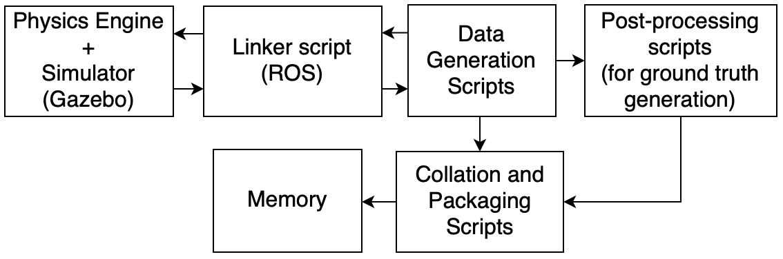
Figure 1: Worflow of the Dataset Generation Simulator

3.1 Dataset Generation Environment

As mentioned earlier, to ensure that we create an environment that resembles the real world, Physics Engines are used. Our simulator for dataset generation is built upon an open-source Physics Engine, ”Gazebo” [21] to simulate the vehicle dynamics and flight/motion patterns necessary to record the required data. We chose to use Gazebo due to its popularity in the robotics community and availability of extensive documentation.

For networks trained on our synthetic data to be applicable to the real world, the simulation-to-real gap, discussed further in 3.6, must be as small as possible. A simulated vehicle used for data collection or DCV that is easy to model ensures a low sim-to-real gap without making the model overly complicated. At the same time, the DCV must be modelled on a real world vehicle that is readily available for physical experiments. Such experiments can help to estimate the sim-to-real gap, and also to validate the efficacy of networks trained using our simulated data. Due to the popularity of multi-rotor platforms, we employ a simulated quadcopter for data collection. This quadcopter is modelled to mimic the physical characteristics of the 3DR Iris Quadcopter [3] from Arducopter, due to its ready availability in both physical and simulated form.

To free our data generator scripts from the burden of flight control operations and to ensure steady, level flight, we choose to have a full-fledged flight control stack running in parallel to data collection. This flight control stack must be able to fly the DCV along its assigned path in simulation autonomously, while also facilitating the collection of the required data. It must also be lightweight during operation in order to preserve most of the available compute resources for the data collector script. The PX4 [24] flight control stack running the MAVLINK [10] communication protocol was chosen to fulfill this role due to its lightweight nature, the high degree of customizability it offers, along with extensive documentation supported by a large community of developers.

To handle the communication of sensor data recorded from the simulator, we opted to work with Robot Operating System (ROS) [28] at the backend. ROS integrates seamlessly with Gazebo and the PX4 flight stack and provides easy access to sensor data. To set the pre-planned flight trajectory, we use PX4’s companion ground control station software, QGroundControl [19].

To reduce data loss due to collection and processing delays, all simulations are slowed down by a factor of eight with respect to real time. This slowdown enables the data collection script to capture most of the data generated by the simulated sensors.

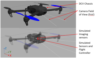
Figure 2: Simulated Quadcopter instrumented with Imaging and Inertial Sensors. The Body frame of reference of the quadcopter is shown in the bottom-left corner

3.2 Simulated Sensors

To record data in the simulated environment, the DCV is instrumented with sensors that are mentioned in Table 2. A reference diagram of the simulated sensor mounts, along with the body frame of reference of the DCV is shown in Fig. 2. All simulated sensors record data in the drone’s body frame.

Sensor	Specifications
VI-sensor	Resolution: 1440x1080 pixels
	@50 fps
	FoV: 60∘ horizontal
Kinect Depth sensor	Resolution: 1440x1080 pixels
	@50 fps
	Sensing limits: [0.1, 500]m
	FoV: 60∘ horizontal
DAVIS	640x480 pixels
	FoV: 60∘ horizontal

Table 2: Specifications of the Simulated Sensors. FoV: Field of View, $fps$: Frames per second

For generating RGB frames, a simulated camera based on the Gazebo Camera driver [1] is mounted on the quadrotor. The simulated camera has a lens with a focal length of $30mm$ and a $60^{\circ}$ horizontal field of view. The camera has a $1440\times 1080$ pixel resolution and a 50 fps output. Each frame sample is timestamped and synchronized with the event and depth streams.

To generate events, an event camera based on the DVS plugin by Kaiser [25, 22, 6] is used. The camera provides events at VGA resolution ($640\times 480$ pixels), and has a theoretical minimum time interval of $0.5ms$ between events, limited by simulator update rate. In practice, however, due to system memory constraints and data processing delays, minimum time intervals closer to $4ms$ have been observed. The event threshold of the simulated event camera is also controllable. This can be exploited to achieve variable event densities. For the sequences we provide as part of this work, the event threshold is set to a value of 30. Recorded events are synchronized with the RGB and depth frames, and are provided in the dataset as metadata. This metadata contains the index of events such that $frame[i]=k$, where $frame[i]$ is the $i^{th}$ RGB or depth frame, and $k$ is the earliest event such that $t_{k}\geq t_{frame[i]}$, where $t_{n}$ is the timestamp of the $n^{th}$ event/frame.

To generate depth, we use the Openni2 [2] driver from Prime Sense. The depth frames have a resolution of $1440\times 1080$ pixels and are encoded using 32-bit single-precision floating-point numbers, with each pixel value representing the measured depth (in mm). To keep the dataset as true to real-world constraints as possible, the depth camera is range limited to a minimum depth of $0.1m$, and a maximum depth of $500m$. Depth values beyond these thresholds are invalid, and are represented by a $NaN$ value.

The field of view of the RGB, depth, and event sensors is intentionally kept identical, so as to ease the generation of the optical flow, as described in Section 4.

Pose is generated using the transform library ”tf” [9]. Pose is computed in the DCV’s body frame of reference, but is internally transformed into the global frame before storage. To ensure that the recorded pose is as close to the real world as possible, Gaussian noise is introduced into the pose data. This provides our dataset with the unique ability of being “controllable” with respect to the noise in our data.

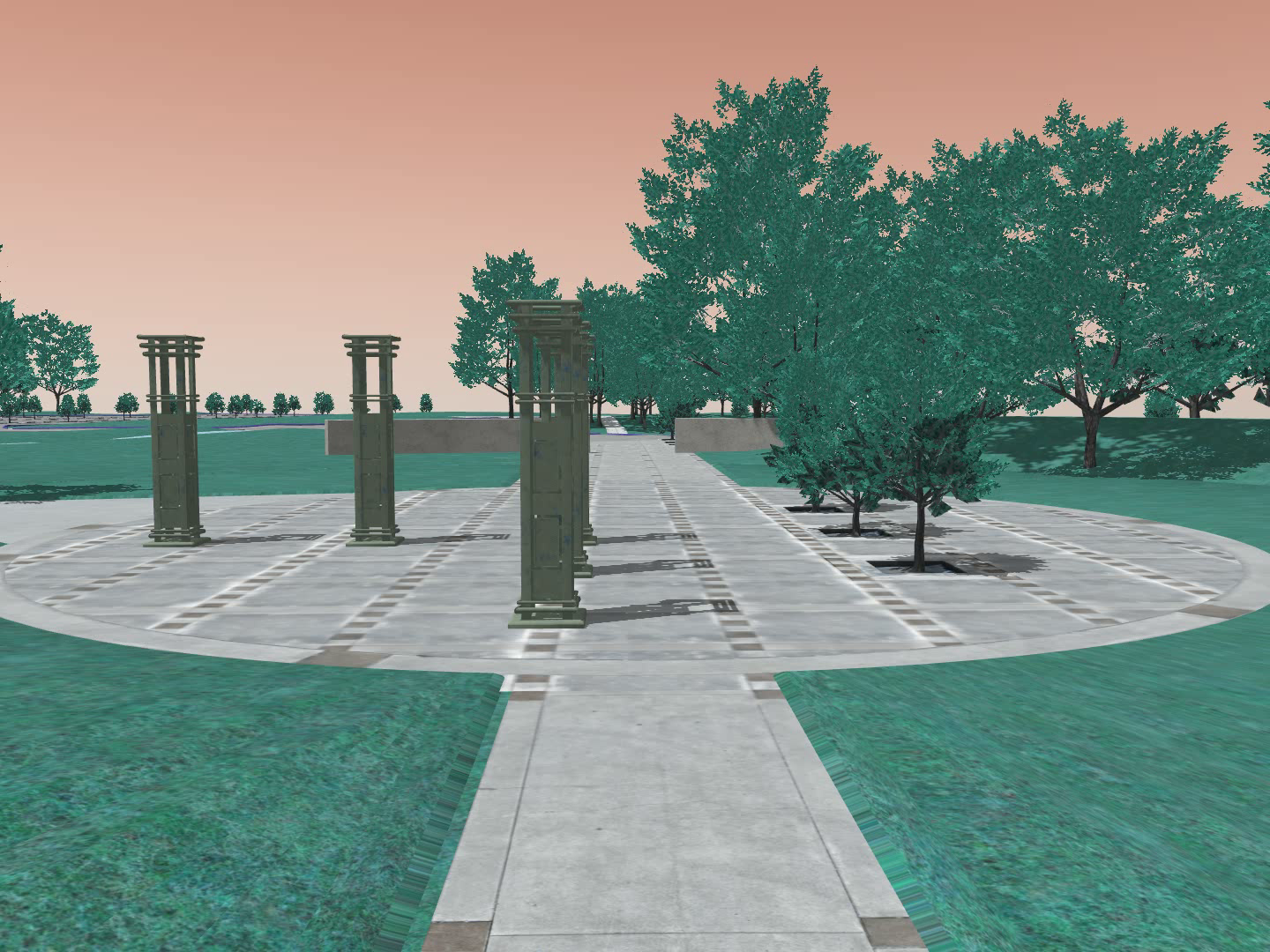
Figure 3: Sample RGB frame from sequence Baylands-Day2

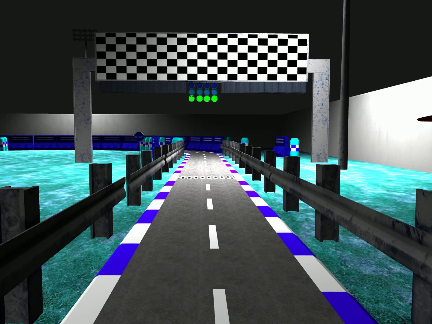
Figure 4: Sample RGB frame from sequence Racetrack-Night

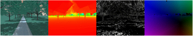
Figure 5: Example RGB and Depth data from the Baylands-Day2 sequence along with the corresponding event and optical flow renders

3.3 Sequences

As part of our dataset, we provide sequences from a variety of environments such as:

1. Baylands: This environment is a true to scale simulation of the Baylands Park in Sunnyvale, CA. We provide sequences from various overflights of the simulated park. Overflights are recorded in varying illumination conditions. Fig. 3 shows a sample frame from the sequence Baylands-Day2.

2. Racetrack: This is an outdoor environment from AWS [29] simulating a racetrack. We provide one daytime and another night time sequence in this environment, both following a survey pattern of the racetrack. Fig. 4 shows an example frame from the sequence Racetrack-Night

Table 3 lists out all the sequences provided along with our dataset, as well as a few related statistics for each of the sequences. Fig. 5 shows a sample color frame along with the corresponding depth and accumulated event frames and the optical flow ground truth.

World	Sequence	T(s)	D(m)	$||v||_{max}$(m/s)	$||\omega||_{max}$(rad/s)	MER(million events/s)
Baylands	Day 1	166	599.52	5.596	0.524	0.65
	Day 2	177	313.436	3.923	0.387	1.13
	Dusk	173	306.19	2.666	0.225	0.907
Racetrack	Day	113	191.35	2.522	0.218	1.24
	Night	116	196.042	2.521	0.294	1.077

Table 3: Sequences provided as part of this work. T: Length of the sequence, D: Total distance travelled by the DCV in the simulated flight, $||v||_{max}$: Maximum aerial velocity attained by the DCV, $||\omega||_{max}$: Maximum angular velocity of the DCV in flight, MER: Mean Event Rate (million events/s)

3.4 Dataset Generation Environments

The Gazebo “worlds” used to generate the dataset were assembled with standard models in the Gazebo library and open-source world models from Amazon Web Services (AWS) [29]. The simulated environment can be precisely controlled in terms of the color, brightness, and diffusivity of its primary light source(s). This enables the recording of both day- and night-time sequences.

3.5 Data Format

We provide our dataset in the form of HDF5 files, with each file containing groups corresponding to the sequences shown in Table 3. Each group, in turn, contains the “ground truth” values for that sequence. Fig. 6 diagrammatically shows this hierarchy.

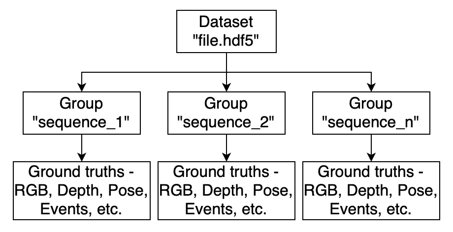
Figure 6: Dataset Storage Hierarchy

We choose the HDF5 format due to its efficient packing fraction [15], and due to its ability to “lazily” load data [14], a highly sought-after quality in RAM-constrained systems. Using a single file to store the dataset also remedies the problems posed by existing datasets, as described in Section 2.

For each of the sequences in our dataset, we provide the following data packed into a Hierarchical Data Format, version 5 (HDF5) [16, 15] file:

• 1440x1080p RGB images at 50fps from a simulated frame camera,

• Inertial measurements from an IMU, at a rate of 50 samples/s.

• Events from a simulated DAVIS sensor [25, 22, 6].

• Depth images from the simulated Prime Sense [8] depth sensor at 50fps.

• Pose data at a rate of 50Hz estimated using the “transform library” (tf) package [9].

• Optical flow generated as described in Section 4.

3.6 Simulation-to-Real Gap

Simulators are subject to different errors due to limitations of the fidelity with which a simulated environment can model the real world. These limitations are usually caused by the use of inaccurate or low-resolution models of simulated objects. Another cause of such limitations are physical phenomena that cannot be accurately modelled, such as random noise.

To mitigate the sim-to-real gap, we try to make the components of our simulation as close to real as possible. To this end, we use state-of-the-art sensor models and model our DCV as accurately as possible. This significantly reduces the sim-to-real gap associated with the DCV and the sensors themselves. In order to reduce the sim-to-real gap associated with the simulated environment, we include models for physical phenomena such as wind in it.

4 Optical Flow Generation

Optical Flow is the apparent motion of a pixel on the 2D image plane due to the movement of object(s) in the observer’s 3D FoV. It can be used for object detection and tracking, background separation, motion detection, and visual odometry.

Due to the wide range of applications for optical flow, we chose to include it as one of our dataset deliverables. We generate optical flow using an analytical approach similar to the one described by Zhu, et al. [34], which uses Eq. 1 and 2 to generate optical flow from the depth and pose estimates obtained from a neural network they proposed.

$$\begin{pmatrix}x_{i}^{*}\\ y_{i}^{*}\end{pmatrix}=K\pi\bigg{(}R\frac{fb}{d_{i}}K^{-1}\begin{pmatrix}x_{i}\\ y_{i}\\ 1\end{pmatrix}+T\bigg{)}$$ (1)

$$\begin{pmatrix}u_{i}\\ v_{i}\end{pmatrix}=\frac{1}{B-1}\bigg{(}\begin{pmatrix}x_{i}^{*}\\ y_{i}^{*}\end{pmatrix}-\begin{pmatrix}x_{i}\\ y_{i}\end{pmatrix}\bigg{)}$$ (2)

$$K=\begin{bmatrix}f_{x}&s&x_{0}\\ 0&f_{y}&y_{0}\\ 0&0&1\end{bmatrix}$$ (3)

Here, $x_{i}^{*}$ and $y_{i}^{*}$ are the new co-ordinates of the pixel $(x_{i},y_{i})$ after application of an affine pose transform which estimates the position of pixel $(x_{i},y_{i})$ due to inter-frame motion. This motion is described by the rotation matrix $R$ and the translation vector $T$. $K$ is the camera intrinsic matrix, $f$ is the focal length of the camera, $b$ is the baseline of the stereo camera setup, $d_{i}$ is the disparity at the $i^{th}$ pixel, and $B$ is the bin count. Zhu, et al. use bins to discretize the temporal dimension as part of their input representation. Thus, they compute optical flow with the unit “pix/bin” instead of the standard unit of “pix/s”. The projection function, given by Eq. 4 and also referred to as the $\pi$ function is used to normalize about the depth axis, which is the $z$-axis in the co-ordinate frame used by Zhu, et al.

$$\pi\begin{pmatrix}x&y&z\end{pmatrix}^{T}=\begin{pmatrix}\frac{x}{z}&\frac{y}{z}\end{pmatrix}^{T}$$ (4)

In the camera intrinsic matrix, given by Eq. 3, $f_{x}$ and $f_{y}$ are the focal lengths of the camera (in pixels) about the $X-$ and $Y-$axes respectively, $s$ is the skew, and $x_{0}$ and $y_{0}$ are the distances (in pixels) of the principal point of the camera (the center of the sensor) from the top-right corner of the sensor. Skew is a measure of the sheer distortion introduced into an image when the $x$ and $y$ axes of the image plane are not perpendicular to each other. In our setup, all three image sensors (RGB, depth, and event) are configured to have a skew of zero.

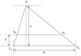
Figure 7: Depth estimation in a Stereo setup. We use Eq. 5 to modify Eq. 1 to generate optical flow

Since we do not use a stereo setup like the one used by Zhu, et al. [34, 33], the baseline $b$ and disparity $d_{i}$ cannot be computed. However, from Fig. 7 and by the laws of similar triangles, we can derive Eq. 5. Using Eq. 5, the scalar term $\dfrac{fb}{d_{i}}$ can be replaced with the depth at the $i^{th}$ pixel, $z_{i}$, which is available to us as a ground truth value.

$$\frac{b}{z_{i}}=\frac{(b+x_{2})-x_{1}}{z_{i}-f}\implies z_{i}=\frac{f.b}{x_{1}-x_{2}}=\frac{f.b}{d_{i}}$$ (5)

The factor $\dfrac{1}{B-1}$ accounts for the number of bins used in the discretization of the time domain. We do not use bins and compute optical flow per unit time. Thus, we can replace the $\dfrac{1}{B-1}$ factor by the inter-frame time of the generated optical flow.

Thus, Eq. 1 and 2 can be rewritten as Eq. 6 and 7.

$$\begin{pmatrix}x_{i}^{*}\\ y_{i}^{*}\end{pmatrix}=K\pi\bigg{(}Rz_{i}K^{-1}\begin{pmatrix}x_{i}\\ y_{i}\\ 1\end{pmatrix}+T\bigg{)}$$ (6)

$$\begin{pmatrix}u_{i}\\ v_{i}\end{pmatrix}=t_{ie}\bigg{(}\begin{pmatrix}x_{i}^{*}\\ y_{i}^{*}\end{pmatrix}-\begin{pmatrix}x_{i}\\ y_{i}\end{pmatrix}\bigg{)}$$ (7)

where $t_{ie}$ is the interval between consecutive optical flow estimates. Eq. 6 holds only when the $z$ axis is the depth direction. However, as shown in Fig. 2, the depth direction of our simulated DCV is the $X$ axis.

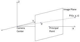
Figure 8: Redefined Pinhole Camera Co-ordinate System for Optical Flow Computation

To accommodate for this change, the pinhole camera model is modified as shown in Fig. 8, yielding a new camera intrinsic matrix, as shown in Eq. 8

$$K=\begin{bmatrix}1&0&0\\ -y_{0}&f_{y}&0\\ z_{0}&0&f_{z}\end{bmatrix}$$ (8)

The change of co-ordinate frame leads to a change in direction on the Y-Axis, which necessitates the negation of the $y_{0}$ component, as seen in Eq. 8. Eq. 6 and 7 are also modified as follows:

$$\begin{pmatrix}y_{i}^{*}\\ z_{i}^{*}\end{pmatrix}=K\pi\bigg{(}Rx_{i}K^{-1}\begin{pmatrix}1\\ y_{i}\\ z_{i}\end{pmatrix}+T\bigg{)}$$ (9)

$$\begin{pmatrix}u_{i}\\ v_{i}\end{pmatrix}=t_{ie}\bigg{(}\begin{pmatrix}y_{i}^{*}\\ z_{i}^{*}\end{pmatrix}-\begin{pmatrix}y_{i}\\ z_{i}\end{pmatrix}\bigg{)}$$ (10)

with the projection function being redefined as in Eq. 11

$$\pi\begin{pmatrix}x&y&z\end{pmatrix}^{T}=\begin{pmatrix}\frac{y}{x}&\frac{z}{x}\end{pmatrix}^{T}$$ (11)

As shown by Gehrig, et al.[11], event data must be rectified if the Fields of View (FoV) of the event and stereo frame cameras used to compute depth are not identical. In our setup, we use a depth camera to measure depth directly. In order to reduce the overhead of event rectification, we design the event and depth cameras to have the same FoV and position both sensors at the same point in simulated space.

The primary advantage of our optical flow generation methodology is the programmability it provides in terms of the rate of the generated optical flow. We provide optical flow for each of our sequences at three different rates - $10fps$, $25fps$, and $50fps$. However, our code may be used to compute optical flow at other frequencies as well.

5 Discussion

A high Degree-of-Freedom (DoF) depth is required to generate a high DoF optical flow with both high temporal resolution, and high range. Since non-flying DCVs have DoF restricted to 3, most existing datasets (DrivingStereo [32], DDAD [17], and Kitti [13]) have only 3-DoF. Although MVSEC [33] and DSEC [11] utilize flying DCVs for some sequences, these sequences are restricted to controlled indoor environments, causing the depth data in these sequences to have little, if any components beyond the standard 3-DoF values.

The sequences in FEDORA on the other hand have been recorded in simulated outdoor environments, and contain depth values along all 6-DoF. This yields data more suited to training depth estimators for flying vehicles. This, in turn, results in a higher DoF optical flow.

The mean value of optical flow provided by DSEC is $7.751$ pix/s, while the mean optical flow values for the Baylands-Day1 and -Day2 sequences in FEDORA are $48.31$ pix/s. Thus, optical flow networks trained on FEDORA are exposed to a larger range of flow, leading to better flow estimation ability over a larger range of flow values.

Another advantage of FEDORA is the high resolution of the depth provided. Some datasets such as DDAD use only LIDARs to estimate depth, thus limiting the resolution of their depth data in both the spatial and temporal domains. Others like DSEC use stereo sensing to compute depth, fundamentally limiting their resolution. FEDORA uses a simulated depth camera to get depth, leading to millimeter accuracy on every valid pixel.

6 Experiments

In order to assess the benefits of temporally dense optical flow, we train a modified version of EvFlowNet proposed by Ponghiran, et al.[27] with our multi-frequency optical flow data. We train the model on $10Hz$, $25Hz$, and $50Hz$ optical flow data from both sequences Baylands-Day1 and Baylands-Day2 together for 80 epochs and a number of learning rates, and choose the best results. Optical flow for all three frequencies is generated over the same time interval to enable an iso-time comparison, and hence test the intuition that higher frequency ground truth leads to better learning. We chose to use the Normalised Average Endpoint Error (NAEE) as the metric for quantifying our results, as the mean optical flow value is different at different frequencies, making comparisons based on the absolute value of the Average Endpoint Error (AEE) an unfair metric. NAEE is computed as

$$\text{NAEE}=\frac{\text{AEE}}{\text{Mean Optical Flow Ground Truth}}$$

The number of training samples in the same sequence is five times greater at $50Hz$ than at $10Hz$. To verify that the high NAEE at $10Hz$ is not caused solely by the smaller number of training samples, the networks are trained on both sequences together, which leads to an increased number of training samples at $10Hz$. Table 4 shows the results from these experiments.

Optical Flow Frequency	AEE	NAEE	Mean Optical Ground Truth(pix/s)
$10$Hz	19.81	0.410	48.31
$25$Hz	11.0	0.379	29.01
$50$Hz	7.754	0.437	17.74

Table 4: Results of training the modified EvFlowNet [27] on our data from sequences Baylands-Day1 and Baylands-Day2.

While the NAEE values for $10Hz$ and $25Hz$ in Table 4 follow the expected trend, an accuracy drop is observed with $50Hz$ data. This indicates that while a higher rate of optical flow leads to better learning, too large a sampling frequency can be detrimental.

7 Limitations

As explained in Section 4, optical flow is computed using Eq. 9 and 10. Eq. 9 and 10 suffer from numerical instability on and in the neighbourhood of invalid pixels. To mitigate this instability, we mark all pixels with flow values of more than a threshold value to be invalid. This threshold is experimentally set to $100$.

As explained in Section 3.6, we have modelled constituents of the simulation to the best of our knowledge. However, due to the difficulty and compute overhead associated with the rendering of complex physical phenomena like the rustling of leaves due to the wind, such phenomena are absent in our simulation environment.

8 Conclusion

This paper presents FEDORA, a first-of-its-kind synthetic dataset for drone operations with VGA-resolution event cameras. In addition, we also provide RGB, depth, pose, ego-motion, and optical flow data, being the first synthetic dataset to provide all these ground truths as part of a single dataset. FEDORA is the first dataset to provide optical flow at three different frequencies.

We believe that this work will serve as the foundation for a new class of datasets that will significantly reduce the number of different datasets required for holistic training and lead to more accurate and energy-efficient networks in the future. We plan to continuously extend this dataset with more ground truths, such as semantic segmentation, and also aim to provide sequences from contextually richer environments with moving objects while, at the same time, reducing the sim-to-real gap.

References

- [1] Wrappers, tools and additional api’s for using ros with the gazebo simulator. https://github.com/ros-simulation/gazebo_ros_pkgs.
- [2] Primesense a subsidiary of Apple Inc. Openni driver. https://github.com/OpenNI/OpenNI.
- [3] Arducopter. Iris: The ready-to-fly uav quadcopter. http://www.arducopter.co.uk/iris-quadcopter-uav.html.
- [4] Francisco Barranco, Cornelia Fermuller, Yiannis Aloimonos, and Tobi Delbruck. A dataset for visual navigation with neuromorphic methods. Frontiers in Neuroscience, 10, 2016.
- [5] Jonathan Binas, Daniel Neil, Shih-Chii Liu, and Tobi Delbruck. Ddd17: End-to-end davis driving dataset, 2017.
- [6] Christian Brandli, Raphael Berner, Minhao Yang, Shih-Chii Liu, and Tobi Delbruck. A 240 × 180 130 db 3 µs latency global shutter spatiotemporal vision sensor. IEEE Journal of Solid-State Circuits, 49(10):2333–2341, 2014.
- [7] Holger Caesar, Varun Bankiti, Alex H. Lang, Sourabh Vora, Venice Erin Liong, Qiang Xu, Anush Krishnan, Yu Pan, Giancarlo Baldan, and Oscar Beijbom. nuscenes: A multimodal dataset for autonomous driving. In CVPR, 2020.
- [8] The Intel Corporation. Intel realsense technology. https://www.intel.com/content/www/us/en/architecture-and-technology/realsense-overview.html.
- [9] Tully Foote. tf: The transform library. In Technologies for Practical Robot Applications (TePRA), 2013 IEEE International Conference on, Open-Source Software workshop, pages 1–6, April 2013.
- [10] The Dronecode Foundation. Mavlink: Micro air vehicle message marshalling library. https://github.com/mavlink/mavlink.
- [11] Mathias Gehrig, Willem Aarents, Daniel Gehrig, and Davide Scaramuzza. Dsec: A stereo event camera dataset for driving scenarios. IEEE Robotics and Automation Letters, 2021.
- [12] Mathias Gehrig, Mario Millhäusler, Daniel Gehrig, and Davide Scaramuzza. E-raft: Dense optical flow from event cameras. In International Conference on 3D Vision (3DV), 2021.
- [13] Andreas Geiger, Philip Lenz, and Raquel Urtasun. Are we ready for autonomous driving? the kitti vision benchmark suite. In Conference on Computer Vision and Pattern Recognition (CVPR), 2012.
- [14] The HDF Group. Documentation of the h5py library. https://docs.h5py.org/en/stable/index.html.
- [15] The HDF Group. Hdf documentation. https://portal.hdfgroup.org/display/support/Documentation?utm_source=hdfhomepage.
- [16] The HDF Group. The hdf5 library and file format. https://www.hdfgroup.org/solutions/hdf5/.
- [17] Vitor Guizilini, Rares Ambrus, Sudeep Pillai, Allan Raventos, and Adrien Gaidon. 3d packing for self-supervised monocular depth estimation. In IEEE Conference on Computer Vision and Pattern Recognition (CVPR), 2020.
- [18] Yuhuang Hu, Jonathan Binas, Daniel Neil, Shih-Chii Liu, and Tobi Delbruck. Ddd20 end-to-end event camera driving dataset: Fusing frames and events with deep learning for improved steering prediction. 2020.
- [19] Dronecode Project Inc. http://qgroundcontrol.com/.
- [20] Jinyong Jeong, Younggun Cho, Young-Sik Shin, Hyunchul Roh, and Ayoung Kim. Complex urban dataset with multi-level sensors from highly diverse urban environments. The International Journal of Robotics Research, 38(6):642–657, 2019.
- [21] N. Koenig and A. Howard. Design and use paradigms for gazebo, an open-source multi-robot simulator. In 2004 IEEE/RSJ International Conference on Intelligent Robots and Systems (IROS) (IEEE Cat. No.04CH37566), volume 3, pages 2149–2154 vol.3, 2004.
- [22] Patrick Lichtsteiner, Christoph Posch, and Tobi Delbruck. A 128 128 120 db 15 s latency asynchronous temporal contrast vision sensor. IEEE Journal of Solid-State Circuits, 43(2):566–576, 2008.
- [23] Will Maddern, Geoff Pascoe, Chris Linegar, and Paul Newman. 1 Year, 1000km: The Oxford RobotCar Dataset. The International Journal of Robotics Research (IJRR), 36(1):3–15, 2017.
- [24] Lorenz Meier, Dominik Honegger, and Marc Pollefeys. Px4: A node-based multithreaded open source robotics framework for deeply embedded platforms. Proceedings - IEEE International Conference on Robotics and Automation, 2015:6235–6240, 06 2015.
- [25] Elias Mueggler, Basil Huber, and Davide Scaramuzza. Event-based, 6-dof pose tracking for high-speed maneuvers. In 2014 IEEE/RSJ International Conference on Intelligent Robots and Systems, pages 2761–2768, 2014.
- [26] Elias Mueggler, Henri Rebecq, Guillermo Gallego, Tobi Delbruck, and Davide Scaramuzza. The event-camera dataset and simulator: Event-based data for pose estimation, visual odometry, and slam. The International Journal of Robotics Research, 36(2):142–149, feb 2017.
- [27] Wachirawit Ponghiran, Chamika Mihiranga Liyanagedera, and Kaushik Roy. Event-based temporally dense optical flow estimation with sequential neural networks, 2022.
- [28] Morgan Quigley, Ken Conley, Brian Gerkey, Josh Faust, Tully Foote, Jeremy Leibs, Rob Wheeler, and Andrew Ng. Ros: an open-source robot operating system. volume 3, 01 2009.
- [29] AWS Robotics. Aws robomaker racetrack world ros package. https://github.com/aws-robotics/aws-robomaker-racetrack-world.
- [30] Pei Sun, Henrik Kretzschmar, Xerxes Dotiwalla, Aurelien Chouard, Vijaysai Patnaik, Paul Tsui, James Guo, Yin Zhou, Yuning Chai, Benjamin Caine, Vijay Vasudevan, Wei Han, Jiquan Ngiam, Hang Zhao, Aleksei Timofeev, Scott Ettinger, Maxim Krivokon, Amy Gao, Aditya Joshi, and Dragomir Anguelov. Scalability in perception for autonomous driving: Waymo open dataset. pages 2443–2451, 06 2020.
- [31] Zhaoning Sun*, Nico Messikommer*, Daniel Gehrig, and Davide Scaramuzza. Ess: Learning event-based semantic segmentation from still images. European Conference on Computer Vision. (ECCV), 2022.
- [32] Guorun Yang, Xiao Song, Chaoqin Huang, Zhidong Deng, Jianping Shi, and Bolei Zhou. Drivingstereo: A large-scale dataset for stereo matching in autonomous driving scenarios. In IEEE Conference on Computer Vision and Pattern Recognition (CVPR), 2019.
- [33] Alex Zihao Zhu, Dinesh Thakur, Tolga Özaslan, Bernd Pfrommer, Vijay Kumar, and Kostas Daniilidis. The multivehicle stereo event camera dataset: An event camera dataset for 3d perception. IEEE Robotics and Automation Letters, 3(3):2032–2039, 2018.
- [34] Alex Zihao Zhu, Liangzhe Yuan, Kenneth Chaney, and Kostas Daniilidis. Unsupervised event-based learning of optical flow, depth, and egomotion. In Proceedings of the IEEE/CVF Conference on Computer Vision and Pattern Recognition (CVPR), June 2019.