Sophia: A Scalable Stochastic Second-order Optimizer for Language Model Pre-training
Abstract
Given the massive cost of language model pre-training, a non-trivial improvement of the optimization algorithm would lead to a material reduction on the time and cost of training. Adam and its variants have been state-of-the-art for years, and more sophisticated second-order (Hessian-based) optimizers often incur too much per-step overhead. In this paper, we propose Sophia, Second-order Clipped Stochastic Optimization, a simple scalable second-order optimizer that uses a light-weight estimate of the diagonal Hessian as the pre-conditioner. The update is the moving average of the gradients divided by the moving average of the estimated Hessian, followed by element-wise clipping. The clipping controls the worst-case update size and tames the negative impact of non-convexity and rapid change of Hessian along the trajectory. Sophia only estimates the diagonal Hessian every handful of iterations, which has negligible average per-step time and memory overhead. On language modeling with GPT models of sizes ranging from 125M to 1.5B, Sophia achieves a 2x speed-up compared to Adam in the number of steps, total compute, and wall-clock time, achieving the same perplexity with 50 fewer steps, less total compute, and reduced wall-clock time. Theoretically, we show that Sophia, in a much simplified setting, adapts to the heterogeneous curvatures in different parameter dimensions, and thus has a run-time bound that does not depend on the condition number of the loss.
1 Introduction
Language models (LLMs) have gained phenomenal capabilities as their scale grows (Radford et al., 2019; Kaplan et al., 2020; Brown et al., 2020; Zhang et al., 2022b; Touvron et al., 2023; OpenAI, 2023). However, pre-training LLMs is incredibly time-consuming due to the massive datasets and model sizes—hundreds of thousands of updates to the model parameters are required. For example, PaLM was trained for two months on 6144 TPUs, which costed 10 million dollars (Chowdhery et al., 2022).
Pre-training efficiency is thus a major bottleneck in scaling up LLMs. This work aims to improve pre-training efficiency with a faster optimizer, which either reduces the time and cost to achieve the same pre-training loss, or alternatively achieves better pre-training loss with the same budget.
Adam (Kingma & Ba, 2014) (or its variants (Loshchilov & Hutter, 2017; Shazeer & Stern, 2018; You et al., 2019)) is the dominantly used optimizer for training LLMs, such as GPT (Radford et al., 2019; Brown et al., 2020), OPT (Zhang et al., 2022b), Gopher (Rae et al., 2021) and LLAMA (Touvron et al., 2023). Designing faster optimizers for LLMs is challenging. First, the benefit of the first-order (gradient-based) pre-conditioner in Adam is not yet well understood (Liu et al., 2020; Zhang et al., 2020; Kunstner et al., 2023). Second, the choice of pre-conditioners is constrained because we can only afford light-weight options whose overhead can be offset by the speed-up in the number of iterations. For example, the block-diagonal Hessian pre-conditioner in K-FAC is expensive for LLMs (Martens & Grosse, 2015; Grosse & Martens, 2016; Ba et al., 2017; Martens et al., 2018). On the other hand, Chen et al. (2023) automatically search among the light-weight gradient-based pre-conditioners and identify Lion, which is substantially faster than Adam on vision Transformers and diffusion models but only achieves limited speed-up on LLMs (Chen et al., 2023).
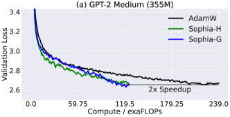
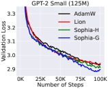
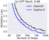
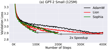
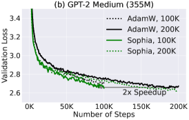
This paper introduces Sophia, Second-order Clipped Stochastic Optimization, a light-weight second-order optimizer that uses an inexpensive stochastic estimate of the diagonal of the Hessian as a pre-conditioner and a clipping mechanism to control the worst-case update size. On pre-training language models such as GPT-2, Sophia achieves the same validation pre-training loss with 50 fewer number of steps than Adam. Because Sophia maintains almost the memory and average time per step, the speedup also translates to 50 less total compute and 50 less wall-clock time (See Figure 1 (a)&(b)). We also note that comparing the run-time to achieve the same loss is a correct way to compare the speed of optimizers for LLMs; see Section 3.2 for more details.
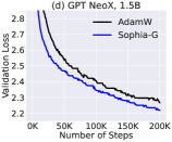
Moreover, the scaling law based on model size from 125M to 770M is in favor of Sophia over Adam—the gap between Sophia and Adam with 100K steps increases as the model size increases (Figure 1 (c)). In particular, Sophia on a 540M-parameter model with 100K steps gives the same validation loss as Adam on a 770M-parameter model with 100K steps. Note that the latter model needs 40% more training time and 40% more inference cost.

Concretely, Sophia estimates the diagonal entries of the Hessian of the loss using a mini-batch of examples every step (with in our implementation). We consider two options for diagonal Hessian estimators: (a) an unbiased estimator that uses a Hessian-vector product with the same run-time as a mini-batch gradient up to a constant factor, and (b) a biased estimator that uses one mini-batch gradient calculated with resampled labels. Both the two estimators only introduce 5% overheads per step (in average). At every step, Sophia updates the parameter with an exponential moving average (EMA) of the gradient divided by the EMA of the diagonal Hessian estimate, subsequently clipped by a scalar. (All operations are element-wise.) See Algorithm 3 for the pseudo-code.
Additionally, Sophia can be seamlessly integrated into existing training pipelines, without any special requirements on the model architecture or computing infrastructure. With the either of the Hessian estimators, Sophia only require either standard mini-batch gradients, or Hessian-vector products which are supported in auto-differentiation frameworks such as PyTorch (Paszke et al., 2019) and JAX (Bradbury et al., 2018).
Thanks to the Hessian-based pre-conditioner, Sophia adapts more efficiently, than Adam does, to the heterogeneous curvatures in different parameter dimensions, which can often occur in the landscape of LLMs losses and cause instability or slowdown. Sophia has a more aggressive pre-conditioner than Adam—Sophia applies a stronger penalization to updates in sharp dimensions (where the Hessian is large) than the flat dimensions (where the Hessian is small), ensuring a uniform loss decrease across all parameter dimensions. In contrast, Adam’s updates are mostly uniform across all parameter dimensions, leading to a slower loss decrease in flat dimensions. (See Section 2.1 for more discussions.) These make Sophia converge in fewer iterations. Thanks to the light-weight diagonal Hessian estimate, the speed-up in the number of steps translates to a speed-up in total compute and wall-clock time.
Sophia’s clipping mechanism controls the worst-case size of the updates in all directions, safeguarding against the negative impact of inaccurate Hessian estimates, rapid Hessian changes over time, and non-convex landscape (with which the vanilla Newton’s method may converge to local maxima or saddle points instead of local minima). The safeguard allows us to estimate Hessian infrequently (every step) and stochastically. In contrast, prior second-order methods often update Hessian estimates every step (Martens & Grosse, 2015; Grosse & Martens, 2016; Anil et al., 2020; Yao et al., 2021).
We provide theoretical analyses of much simplified versions of Sophia on convex functions. The runtime bound does not depend on the local condition number (the ratio between maximum and minimum curvature at the local minimum) and the worst-case curvature (that is, the smoothness parameter), demonstrating the advantage of Sophia in adapting to heterogeneous curvatures across parameter dimensions.
2 Method
We first instantiate gradient descent (GD) and Adam on a simplified 2D problem and motivate the use of second-order information and per-coordinate clipping in Section 2.1. Then, we present Sophia in detail in Section 2.2, and the pseudo-code in Algorithm 3. We introduce two choices of estimators of diagonal Hessian used in Sophia in Section 2.3.
2.1 Motivations
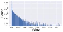
Heterogeneous curvatures. The loss functions of modern deep learning problems often have different curvatures across different parameter dimensions (Sagun et al., 2016; Ghorbani et al., 2019; Zhang et al., 2020; Yao et al., 2020). E.g., on a 125M-parameter GPT-2 model, Figure 3 shows that the distribution of positive diagonal entries of the Hessian is dispersed.
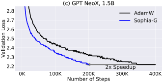
We demonstrate the limitations of Adam and GD on heterogeneous landscapes by considering a two-dimensional loss function where is much sharper than . We plot the loss landscape of in Figure 2.111Concretely, in Figure 2, and . For simplicity, we discuss GD and deterministic versions of Adam. Recall that GD’s update in this setting is:
| (1) |
A common simplification of Adam that is more amenable to analysis (Balles & Hennig, 2018; Bernstein et al., 2018; Zhuang et al., 2020; Kunstner et al., 2023) is SignGD, which dates back to RProp (Braun & Riedmiller, 1992) that motivated RMSProp (Hinton et al., 2012) and Adam. Observe that without using the EMA (for both the gradient and second moments of the gradient), Adam’s update is simplified to (where all operations are entry-wise), which is called SignGD. Applying the update rule to our setting gives:
| (2) |
Limitations of GD and SignGD (Adam). It is well known that the optimal learning rate of GD should be proportional to the inverse of the curvature, that is, the Hessian/second derivative at the local minimum. More precisely, let and be the curvatures of and at the local minimum (and thus ). The optimal learning rate for the update of in equation (1) is , which is much smaller than the optimal learning rate that the update of needs, which is . As a result, the largest shared learning rate can only be ; consequently, the convergence in dimension is slow as demonstrated in the brown curve in Figure 2.
The update size of SignGD is the learning rate in all dimensions. The same update size translates to less progress in decreasing the loss in the flat direction than in the sharp direction. As observed from the yellow curve in Figure 2, the progress of SignGD in the flat dimension is slow because each step only decreases the loss slightly. On the other hand, along the direction , the iterate quickly travels to the valley in the first three steps and then starts to bounce. To fully converge in the sharp dimension, the learning rate needs to decay to 0, which will exacerbate the slow convergence in the flat dimension . The trajectory of Adam in this example is indeed similar to SignGD, which is also plotted as the red curve in Figure 2.
The behavior of SignGD and Adam above indicates that a more aggressive pre-conditioning is needed—sharp dimensions should have relatively smaller updates than flat dimensions so that the decrease of loss is equalized in all dimensions. As suggested by well-established literature on second-order optimization (Boyd & Vandenberghe, 2004) for convex functions, the optimal pre-conditioner should be the Hessian, which captures the curvature on each dimension; as in Newton’s method, the update is the gradient divided by the Hessian in each dimension:
| (3) |
Limitations of Newton’s method. Nevertheless, Newton’s method has known limitations as well. For non-convex functions, vanilla Newton’s method could converge to a global maximum when the local curvature is negative. In the blue curve of Figure 2, Newton’s method quickly converges to a saddle point instead of a local minimum. The curvature might also change rapidly along the trajectory, making the second-order information unreliable. To address these limitations, we propose considering only pre-conditioners that capture positive curvature, and introduce a pre-coordinate clipping mechanism to mitigate the rapid change of Hessian (more detail in Section 2.2). Applying our algorithm on the toy case results in the following update:
| (4) |
where is a constant to control the worst-case update size, is a very small constant (e.g., 1e-12), which avoids dividing by 0. When the curvature of some dimension is rapidly changing or negative and thus the second-order information is misleading and possibly leads to a huge update before clipping, the clipping mechanism kicks in and the optimizer defaults to SignGD (even though this is sub-optimal for benign situations). Numerous prior methods such as trust region (Conn et al., 2000), backtracking line search (Boyd & Vandenberghe, 2004), and cubic regularization (Nesterov & Polyak, 2006) also tackle the same issue of Newton’s method, but the clipping mechanism is much simpler and more efficient.
As shown in the black curve in Fig. 2, the update in equation (4) starts off similarly to SignGD due to the clipping mechanism in the non-convex region, making descent opposed to converging to a local maximum. Then, in the convex valley, it converges to the global minimum with a few steps. Compared with SignGD and Adam, it makes much faster progress in the flat dimension (because the update is bigger in dimension ), while avoiding boucing in the sharp dimension (because the update is significantly shrunk in the sharp dimension ).
2.2 Sophia: Second-order Clipped Stochastic Optimization
Section 2.1 demonstrates that Adam does not sufficiently adapt to the heterogeneous curvatures. On the other hand, vanilla Newton’s method has a pre-conditioner optimal for convex functions, but is vulnerable to negative curvature and rapid change of Hessian. With these insights, we design a new optimizer, Sophia, which is more adaptive to heterogeneous curvatures than Adam, more resistant to non-convexity and rapid change of Hessian than Newton’s method, and also uses a low-cost pre-conditioner.
We use to denote the parameter at time step . At each step, we sample a mini-batch from the data distribution and calculate the mini-batch loss, denoted by . We denote by the gradient of , i.e. . Let be the EMA of gradients, , which is the numerator of the update.
EMA of diagonal Hessian estimates. Sophia uses a diagonal Hessian-based pre-conditioner, which directly adjusts the update size of different parameter dimensions according to their curvatures. We will present two options in detail in Section 2.3 for estimating the diagonal Hessian efficiently. To mitigate the overhead, we only estimate the Hessian every steps ( in our implementation). At time step with , the estimator returns an estimate of the diagonal of the Hessian of the mini-batch loss.
Similar to the gradient of the mini-batch loss function, the estimated diagonal Hessian can also have large noise. Inspired by the EMA of moments of gradients in Adam, we also denoise the diagonal Hessian estimates with EMA across iterations. We update the EMA every steps, resulting in the following update rule for the diagonal Hessian estimate:
| (5) |
Per-coordinate clipping. As discussed in Section 2.1, on nonconvex functions, vanilla Newton’s method, which uses Hessian as the pre-conditioner, may converge to local maxima instead of local minima. In addition, the inaccuracy of Hessian estimates and the change of Hessian along the trajectory can make the second-order information unreliable. To this end, we (1) only consider the positive entries of the diagonal Hessian and (2) introduce per-coordinate clipping to the update. For a clipping threshold , let the clipping function be where all operations are applied coordinate-wise. The update rule is written as:
| (6) |
where is a very small constant to avoid dividing by . Note that , and thus we essentially clip the original update by coordinate-wise, and then re-adjust the final update size by a factor of . The re-adjustment makes the scale of the update less dependent on , because now only controls the fraction of clipped entries but all clipped entries will eventually be set to in the udpate—e.g., when is extremely small, all entries of will be . In practice, the choice of should be tuned based on the the fraction of clipped entries (See Section 3.1 for details). We present the pseudo-code of the Sophia in Algorithm 3.
When any entry of is negative, e.g., , the corresponding entry in the pre-conditioned gradient is extremely large and has the same sign as , and thus , which is the same as stochastic momentum SignSGD. In other words, Sophia uses stochastic momentum SignSGD as a backup when the Hessian is negative (or mistakenly estimated to be negative or very small.) We also note that the clipping mechanism controls the worst-case size of the updates in all parameter dimensions to be at most , which also improves the stability (which could be a severe issue for second-order methods). Moreover, because for many parameter dimensions, the clipping is not activated and the update is automatically adjusted, our worst-case update size can be chosen to be larger than the worst update size in stochastic momentum SignSGD.
Several previous works (Becker & Le Cun, 1988; Chapelle et al., 2011; Schaul et al., 2013), including the recent work AdaHessian (Yao et al., 2021), use diagonal Hessian as a pre-conditioner in optimizers for training neural networks. However, they use more frequent Hessian estimations, which leads to significant per-step computation overhead (more than two gradient computations), most likely because of the lack of the clipping mechanism that safeguards against inaccurate and changing Hessian. In general, to the best of our knowledge, there has not been previous reports that showed second-order optimizers achieve a speed-up on decoder-only large language models in wall-clock time or total compute (see more related work and discussions in Section 5).
2.3 Diagonal Hessian Estimators
We introduce two diagonal Hessian estimators, both of which have memory and run-time costs similar to computing a gradient (up to constant factors).
Option 1: Hutchinson’s unbiased estimator. For any loss function on parameters , the Hutchinson’s estimator (Hutchinson, 1989; Roosta-Khorasani & Ascher, 2015; Yao et al., 2021) first draws from the spherical Gaussian distribution , and then outputs , where denotes the element-wise product, and is the product of the Hessian with the vector . The Hutchinson’s estimator is an unbiased estimator for the diagonal of the Hessian, because
| (7) |
The estimator only requires a Hessian-vector product (i.e., ), which have efficient implementations in PyTorch and JAX, instead of the full Hessian matrix.
Option 2: Gauss-Newton-Bartlett (GNB) estimator. We leverage the structure of the loss to design a biased stochastic estimator for the diagonal Hessian, following Schraudolph (2002); Martens (2020); Wei et al. (2020). Suppose is a loss function on an example of the form where is the cross-entropy loss and is the logits, and is the number of items/classes in a multi-class classification problem (e.g., the vocabulary size in LLMs). First, the Hessian of (w.r.t to variable ) has the well-known Gauss-Newton decomposition (Ortega & Rheinboldt, 2000; Schraudolph, 2002) (which is a simple consequence of the chain rule),
| (8) |
where is the Jacobian of w.r.t to viewed as a matrix in , is the second-order derivatives of the loss w.r.t to the logits, is the first-order derivatives of the loss w.r.t to the logits, and is the second-order derivatives of the multi-variate function w.r.t , viewed as a linear map from to , where is the dimension of the parameter .
In the context of neural networks, past works have found that the second term in Equation 8 is often relative smaller than the first term (Sankar et al., 2021), which is often referred to as the Gauss-Newton matrix (Dennis Jr & Schnabel, 1996; Ortega & Rheinboldt, 2000; Schraudolph, 2002; Chen, 2011) and used as pre-conditioners in second-order optimizers (Botev et al., 2017; Martens, 2020; Gargiani et al., 2020). Following this line of work, we build an unbiased estimator for the diagonal of the Gauss-Newton matrix, which is a biased estimator for the diagonal of the Hessian.
We first claim that only depends but not , even though the loss depends on .222Denote by the probability vector obtained by applying softmax on the logits. Indeed, a simple derivation shows that , where is the matrix with the vector residing on the diagonal. In fact, this is a general property of exponential families—the Hessian of the negative log-likelihood of any exponential family distribution only depends on the parameters of that exponential family, but not on the example on which the likelihood is evaluated. Thus, for any , which implies that Because is the negative log-probability of the probabilistic model defined by the categorical distribution with parameter , by Bartlett’s second identity (Bartlett, 1953), we have that,
| (9) |
where the first equality holds for and the second equality holds for all by Bartlett’s second identity. Therefore, the Gauss-Newton matrix satisfies
| (10) |
which implies that . Hence, the quantity is an unbiased estimator of the Gauss-Newton matrix for the Hessian of a one-example loss .
Mini-batch version. Given a mini-batch of inputs . The most natural way to build an estimator for the diagonal of the Gauss-Newton matrix for the Hessian of the mini-batch loss is using
| (11) |
where ’s are labels sampled from the model on inputs ’s respectively. However, as noted by Grosse (2022), implementing this estimator is inconvenient under the current auto-differentiation frameworks, where the users only have access to the average gradient over a mini-batch (as opposed to the individual ones). Fortunately, by the Bartlett’s first identity (Bartlett, 1953) (which generally holds for the negative log-likelihood loss of any probabilistic model), we have:
| (12) |
Let be the mini-batch loss on the sampled labels (as opposed to the original labels). Observing that ’s are independent with each other, we have
| (13) |
Note that the RHS of Equation 13 is the same as the expectation of Equation 11, which, by Equation 10, also equals to the diagonal of the Gauss-Newton matrix for the mini-batch loss. Hence, we use as the estimator.
GNB estimator for exponential family. If is drawn from an exponential family where the natural parameter is set to be and the loss function is the negative log-likelihood loss for the corresponding probabilistic distribution, then all the derivations above still follow because (1) still only depends on but not , and (2) both the first and second Bartlett’s identities still hold.
GNB estimator for squared loss. When and , the matrix is identity, and thus one can simply use as the estimator.333One can verify that the GNB estimator gives the same quantity in expectation if we use a probabilistic model and go through the derivation of the GNB estimator.
To the best of our knowledge, Wei et al. (2020) is the first paper that uses this estimator of Gauss-Newton matrix. Given the use Bartlett’s first and second identities that are central to the estimator, we call it Gauss-Newton-Bartlett (GNB) estimator.
Comparisons of Hessian estimators. The Hutchinson’s estimator does not assume any structure of the loss, but requires a Hessian-vector product. The GNB estimator only estimates the Gauss-Newton term but always gives a positive semi-definite (non-negative) diagonal Hessian estimate. The PSDness ensures that the pre-conditioned update is always a descent direction (Dennis Jr & Schnabel, 1996). The GNB estimator can also be easily extended to the negative log-likelihood loss of any exponential family distribution, and be adapted to estimating the trace of the Gauss-Newton matrix as in Wei et al. (2020) or efficiently implementing the product of Gauss-Newton matrix with a vector. The authors suspect the GNB estimator has a smaller variance than the Hutchinson’s estimator, but more empirical and theoretical investigation are needed to support the hypothesis.
3 Experiments
We name the algorithm using the Hutchinson’s estimator and the GNB estimator Sophia-H and Sophia-G, respectively. We evaluate Sophia on auto-regressive language modeling with GPT-2 (Radford et al., 2019) of model sizes ranging from 125M to 770M, and GPT NeoX (Black et al., 2022) of sizes 1.5B and 6.6B. Results indicate that Sophia is 2x faster than AdamW (Loshchilov & Hutter, 2017) in number of steps, total compute, and wall-clock time across all model sizes. Moreover, the scaling law is in favor of Sophia over AdamW.
3.1 Experimental Setup
Language modeling. We train autoregressive models on OpenWebText (Gokaslan & Cohen, 2019) and the Pile (Gao et al., 2020). Following standard protocol, we set the context length of GPT-2 to 1024, and the context length of GPT-2 NeoX (Black et al., 2022) to 2048. We consider GPT-2 with 125M (small), 355M (medium), and 770M (large) parameters, and GPT NeoX with 1.5B and 6.6B parameters, respectively. Detailed model configurations are deferred to Section B.2.
Baselines. We mainly compare Sophia and Adam with decoupled weight decay (AdamW) (Loshchilov & Hutter, 2017) which is the dominantly used optimizer on language modeling tasks, AdaHessian (Yao et al., 2021) which uses the EMA of the square of the diagonal Hessian estimate in its denominator, and Lion (Chen et al., 2023), which is an first-order adaptive optimizer discovered by symbolic search. For the 30M model, all hyperparameters are tuned with grid search. For other models, all hyperparmeters but the peak learning rate are configured as identical to those found on the 30M model. For models with size 125M and 355M, the peak learning rates are obtained through grid search. For larger models, we gradually increase the peak learning rate to search for the largest possible peak learning rate such that the training does not blow up, and ensure that the chosen learning rate is approximately the largest in the sense that 1.25 times the chosen learning rate will lead to a blow-up. For AdamW we found the well-established practice ( and ) works consistently better than other choices (Radford et al., 2019; Karamcheti et al., 2021). For Lion, we use and following Chen et al. (2023). Although Chen et al. (2023) suggests using times the learning rate (LR) of AdamW for vision tasks, we find out the LR should be larger on LMs from the grid search. For AdaHessian, we found and works the best in the grid search. Details on hyperparameter tuning are deferred to Section B.1.
Implementation. We set batch size to 480 for GPT-2 and 2048 for GPT NeoX. We use cosine LR schedule with the final LR equal to 0.05 times the peak LR, following Rae et al. (2021). We use the standard gradient clipping (by norm) threshold 1.0. We adopt a fixed 2k steps of LR warm-up. For Sophia, we use , , 1e-12 and update diagonal Hessian every 10 steps. For Sophia-H, we use only a subset of 32 examples from the mini-batch to calculate the diagonal Hessian to further reduce overhead. For Sophia-G, we use a subset of 240 examples from the mini-batch to calculate the diagonal Gauss-Newton. We implement the algorithms in PyTorch (Paszke et al., 2019) and JAX (Bradbury et al., 2018) and train all the models in bfloat16. The 125M and 355M models are trained on A5000 GPUs, while the 770M models are trained on A100 GPUs. We use a TPU v3-128 slice to train the 1.5B and 6.6B GPT NeoX.
Hyperparamter tuning strategy.
We refer to Section B.1 for the details on hyperparameters and only discuss two key hyperparameters, and the peak learning rate in the main text. Similar to the protocol of baselines, all other hyperparameters are tuned on a 30M model and remain fixed for all the model sizes. For the peak learning rate and , we found the following strategy general works well, and delivers almost the same performance as those found by grid search.
-
•
On a small model, tune to make the proportion of coordinates where the update is not clipped (i.e., ) in the range of . If the proportion is too large (or too small), multiply by (or ) and restart. The same likely can be transferred to models with the same architecture and data but different number of parameters. We use for Sophia-H and for Sophia-G in this paper.
-
•
Suppose we already find a suitable following the above procedure. We can then set the learning rate of Sophia to be either 3-5 times the learning rate that one would have used for Lion, or 0.8 times the learning rate that one would have used for AdamW.
3.2 Evaluation
Methodology for comparing the optimizers for LLMs.
This paper argues that one correct (and arguably preferred) way of claiming optimizer is 2x faster than optimizer is comparing the following two experiments (for a reasonable variety of ):
-
1.
running optimizer (e.g. Adam) with steps, with the optimal learning rate and learning rate schedule (tuned for running for steps),
-
2.
running optimizer (e.g., Sophia) with steps, with any learning rate schedule.
If Experiment 2 achieves a loss that is smaller than or equal to the loss of Experiment 1 (for a reasonable sets of choices of ), then we say optimizer is 2x faster than optimizer .
In more formal language, suppose the loss (or any minimization metric) of an optimizer with runtime budget and hypeparameter (excluding the runtime ) is denoted by . Then, we say optimizer is -times faster than if
| (14) |
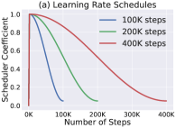
Note that the equation above implies , but is simpler to verify than the latter. We note that many modern learning rate schedulers such as cosine learning rate (Loshchilov & Hutter, 2016) are highly sensitive to a pre-specific total number of steps. The optimal hyperparameters are also sensitive to the total budget . Thus, tuning the hyperparameters of the baseline with a pre-specified budget (aka, minimizing given ) is critical to ensure fair comparison. (On the other hand, the tuning strategy for is less important because we just need to show the existence of a good .)
Moreover, we note that, in equation (14), we need to insist without any approximations. The difference in losses of various experiments might be seemingly small— is likely to be only slightly higher than (assuming the peak learning rate is a hyperparameter), and thus allowing any approximation in the criterion (14) may lead to the fallacy statement that “Adam is 2x faster than Adam”. In fact, Figure 4 (a) shows that even with the same peak learning rate, the learning rate in a run with steps decays faster than the learning rate in a run with steps. Moreover, the -steps run tends to have a initial faster decay of loss than the -steps run but stop at a higher final loss, and the latter is not a continuation of the former.
Finally, a tempting comparison would be comparing the following experiment with Experiment 1:
-
2’.
running optimizer (e.g., Sophia) with steps, with any learning rate schedule, and recording the performance of the -th checkpoint.
We note that if one were able to find an optimizer that is 2x faster than under the proposed criterion (comparing 1&2), then one can also design another optimizer (which run for steps) that is 2x faster than under the second criterion (comparing 1&2’): first running optimizer for steps and do nothing for the rest of the steps. Therefore, even though we will also provide comparison between Experiment 1&2’ in Figure 5 as an alternative, we use the comparison between Experiment 1&2 quantitatively in most of the paper.
Technical details.
Following the methodology above, we train baselines and Sophia for 100K, 200K, or 400K, and mainly compare 400k-steps baseline vs 200K-steps Sophia, and 200k-steps baseline vs 100k-steps Sophia. We primarily evaluate the models with their log perplexity and plot the loss curves. We also report in-context learning results (with 2-shot exemplars and greedy decoding) on SuperGLUE (Wang et al., 2019). We average the results of 5 prompts (Section B.3).

3.3 Results
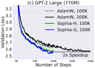
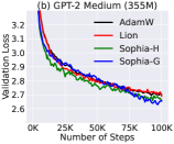
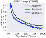
Figure 5 illustrates the validation loss curve (token-level log perplexity) on OpenWebText or the Pile with the same number of steps. Sophia-H and Sophia-G consistently achieve better validation loss than AdamW, Lion, and AdaHessian, while Sophia-G is better than Sophia-H. As the model size grows, the gap between Sophia and baselines also becomes larger. Note that the cost of each step AdaHessian is more than 2x that of AdamW, while Sophia only introduces a per step compute overhead of less than 5. Sophia-H and Sophia-G both achieve a 0.04 smaller validation loss on the 355M model (Figure 5 (b)). Sophia-G and Sophia-H achieve a 0.05 smaller validation loss on the 770M model (Figure 5 (c)), with the same 100K steps. This is a significant improvement since according to scaling laws in this regime (Kaplan et al., 2020; Hoffmann et al., 2022) and results in Figure 4, an improvement in loss of 0.05 is equivalent to 2x improvement in terms of number of steps or total compute to achieve the same validation loss.
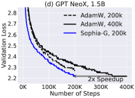
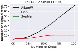
Sophia is 2x faster in terms of number of steps, total compute and wall-clock time. The improvement in validation loss brought by Sophia can be translated into reduction of number of steps or total compute. In Figure 1 (a)(b)(c) and Figure 4, we evaluate the optimizers by comparing the number of steps or total compute needed to achieve the same validation loss level. As can be observed in Figure 1 (a)(b)(c), Sophia-H and Sophia-G achieve a 2x speedup compared with AdamW and Lion across different model sizes.
The scaling law is in favor of Sophia over AdamW. In Figure 1 (d), we plot the validation loss on OpenWebText of models of different sizes pre-trained for 100K steps. The gap between Sophia and AdamW grows as we scale up the models. Moreover, the 540M model trained by Sophia-H has smaller loss than the 770M model trained by AdamW. The 355M model trained by Sophia-H has comparable loss as the 540M model trained by AdamW.
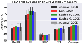
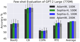
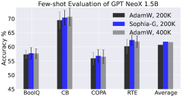
Few-shot Evaluation on Downstream Tasks (SuperGLUE). As shown in Figure 6, as expected, the improvement in validation loss transfers to an improvement in downstream task accuracy. With the same number of steps in pre-training, GPT-2 medium, GPT-2 large and GPT NeoX 1.5B pre-trained with Sophia have better few-shot accuracy on most subtasks. Also, models pre-trained with Sophia have comparable few-shot accuracy as models pre-trained with AdamW for 2x number of steps.
3.4 Analysis
| Algorithm | Model Size | T(step) | T(Hessian) | Compute |
|---|---|---|---|---|
| AdamW | 770M | 3.25s | – | 2550 |
| Sophia-H | 770M | 3.40s | 0.12s | 2708 |
| Sophia-G | 770M | 3.42s | 0.17s | 2678 |
| AdamW | 355M | 1.77s | – | 1195 |
| Sophia-H | 355M | 1.88s | 0.09s | 1249 |
| Sophia-G | 355M | 1.86s | 0.09s | 1255 |
Comparison of wall-clock time and amount of compute. We compare the total compute (TFLOPs) per step and the wall-clock time on A100 GPUs in Table 1. We report the average time per step (T(step)), the time spent in Hessian computation (T(Hessian)) and the total compute following Chowdhery et al. (2022). Since we calculate the diagonal Hessian estimate with a reduced batch size every 10 steps, the computation of the Hessian accounts for 6 of the total compute, and the overall wall-clock time overhead is less than 5 compared with AdamW. In terms of memory usage, our optimizer has two states, and , which results in the same memory cost as AdamW.
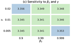
Sensitivity to and , and transferability of hyperparameters. On a 30M model, we perform a grid search to test the sensitivity of Sophia-H to hyperparamters (Figure 7 (c)). All combinations have a similar performance, while and performs the best. Moreover, this hyperparameter choice is transferable across model sizes. For all the experiments on 125M, 355M and 770M, we use the hyperparameters searched on the 30M model, which is , .
Training Stability. Sophia-H has better stability in pre-training compared to AdamW and Lion. Gradient clipping (by norm) is an important technique in language model pre-training as it avoids messing up the moment of gradients with one mini-batch gradient computed from rare data (Zhang et al., 2020). In practice, the frequency that gradients clipping is triggered is related to the training stability—if the gradient is frequently clipped, the iterate can be at a very instable state. We compare the proportion of steps where gradient clipping is triggered on GPT-2 small (125M) in Figure 7 (a). Although all methods use the same clipping threshold 1.0, Sophia-H seldomly triggers gradient clipping, while AdamW and Lion trigger gradient clipping in more than 10 of the steps.
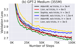
Another common trick of pre-training deep Transformers is scaling the product of keys and values by the inverse of the layer index as implemented by Mistral (Karamcheti et al., 2021) and Huggingface (Wolf et al., 2020). This stabilizes training and increases the largest possible learning rate. Without this trick, the maximum learning rate of AdamW and Lion on GPT-2 medium (355M) can only be 1.5e-4, which is much smaller than 3e-4 with the trick (the loss will blow up with 3e-4 without the trick). Moreover, the loss decreases much slower without the trick as shown in Figure 7 (b). In all the experiments, Sophia-H does not require scaling the product of keys and values by the inverse of the layer index.
3.5 Ablation Study
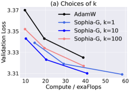
Choices of Hessian update frequency . We study the effect of Hessian update frequency of Sophia-G on computational overhead and validation loss on a 30M GPT-2 model. We consider and run each method for 100k, 200k, and 400k steps. All other hyperparameters are fixed, and we tune the peak learning rate with a grid search. We plot the amount of compute spent and the validation loss of each run in Figure 8 (a). While has better validation loss with the same number of steps, the computational overhead is 50 and the convergence speed with respect to amount of compute is worse than . The choice of still outperforms AdamW, but is not as good as .
Diagonal Hessian pre-conditioners. We compare different diagonal Hessian pre-conditioners (with the same and found by grid search): Empirical Fisher (E-F+clip), AdaHessian (AH+clip), Hutchinson (Sophia-H), and GNB (Sophia-G). Note that empirical Fisher is the EMA of squared gradients, which differs from GNB in label sampling. We run each method for 100k, 200k, and 400k steps and plot the results in Figure 8 (b). Results indicate that GNB is better than Empirical Fisher, which is consistent with Kunstner et al. (2019). Sophia-H is also consistently better than AdaHessian. We hypothesize that the difference stems from that the EMA of the diagonal Hessian estimates (used in Sophia-H ) has more denoising effect than the EMA of the second moment of Hessian estimates (used in AdaHessian).
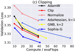
Element-wise Clipping. We compare the role of different update clipping strategy in Figure 8 (c). We include element-wise clipping without pre-conditioners (Clip), update normalization without pre-conditioners (Normalize), AdaHessian and Sophia-G without clipping (GNB). The learning rate is found by grid search. Note that clipping without pre-conditioner is essentially the same as sign momentum, or Lion with a single . Without element-wise clipping, we find that AdaHessian will diverge with and GNB will diverge with , thus we use for AdaHessian and for GNB. Results indicate that per-coordinate clipping itself is already better than AdamW. Further adding the GNB pre-conditioner makes Sophia-G much better than baselines.
4 Theoretical Analysis
This section provides runtime bounds for the deterministic version of Sophia that does not depend on the local condition number (the ratio between maximum and minimum curvature at the local minimum) and the worst-case curvature (that is, the smoothness parameter), demonstrating the advantage of Sophia in adapting to heterogeneous curvatures across parameter dimensions.
We start with standard assumptions on the differentiability and uniqueness of the minimizer.
Assumption 4.1.
is a twice continuously differentiable, strictly convex function with being its minimizer. For convenience, we denote by .
The following assumptions state that the Hessian has a certain form of continuity—within a neighborhood of size , the ratio between the Hessians, , is assumed to be bounded by a constant 2.
Assumption 4.2.
There exists a constant , such that
| (15) |
We analyze the convergence rate of the deterministic version of the Sophia on convex functions,
| (16) |
where is an eigendecomposition of . Here, we use the full Hessian as the pre-conditioner because the diagonal Hessian pre-conditioner cannot always work for general functions which may not have any alignment with the natural coordinate system. Moreover, the matrix transforms into eigenspace and thus the clipping can be done element-wise in the eigenspace. We do not need the max between Hessian and in the original version of Sophia because the Hessian is always PSD for convex functions. Finally, the matrix transforms the update back to the original coordinate system for the parameter update.
Theorem 4.3.
Under 4.1 and 4.2, let , the update in Equation 16 reaches a loss at most in steps.
The first term in the runtime bound is a burn-in time before reaching a local region, where the error decays exponentially fast so that the runtime bound is logarithmic in as the second term in the runtime bound shows. We remark that the bound does not depend on the condition number (the ratio between the maximum and minimum eigenvalue of Hessian), as opposed to the typical dependency on the maximum eigenvalue of the Hessian (or the smoothness parameter) in standard analysis of gradient descent in convex optimization (Boyd & Vandenberghe, 2004). Moreover, even on simple quadratic functions, the convergence rate of simplified Adam (SignGD) depends on the condition number (Appendix D.1). This demonstrates the advantage of Sophia in adapting to heterogeneous curvatures across parameter dimensions.
5 Related work
Stochastic Adaptive First-order Optimizers in Deep Learning. The idea of adaptive first-order optimizers dates back to RProp (Braun & Riedmiller, 1992). AdaGrad (Duchi et al., 2011) adapted the learning rate of features by estimated geometry and assign larger learning rate to infrequent features. RMSProp (Hinton et al., 2012) generalized RProp and is capable to work with smaller batch sizes. Adam (Kingma & Ba, 2014) improved RMSProp by introducing a running average of gradients, and has so far become the dominant approach to solve optimization problems in deep learning, especially for training Transformers (Vaswani et al., 2017). Many follow-up works proposed variants of Adam (Dozat, 2016; Shazeer & Stern, 2018; Reddi et al., 2019; Loshchilov & Hutter, 2017; Zhuang et al., 2020; You et al., 2019). Chen et al. (2023) performed a search over adaptive first-order algorithms and discovered Lion, which is a improved version of sign momentum SGD.
Second-order Optimizers in Deep Learning. Second-order optimizers are believed to have the potential to outperform adaptive first-order optimizers. Classical second-order optimization algorithms pre-condition the gradient with curvature information (Broyden, 1970; Nesterov & Polyak, 2006; Conn et al., 2000). Over the years, people have developed numerous ways to adapt these methods to deep learning. To the best of our knowledge, Becker & Le Cun (1988) was the first to use diagonal Hessian as the pre-conditioner. Martens et al. (2010) approximated the Hessian with conjugate gradient. Schaul et al. (2013) automatically tuned learning rate of SGD by considering diagonal Hessian. Pascanu & Bengio (2013) considered Gaussian Newton’s approximation of Hessian and Fisher information matrix. Martens & Grosse (2015) and follow-up works (Ba et al., 2017; George et al., 2018; Martens et al., 2018; Zhang et al., 2022a) proposed to approximate the Hessian based on the structure of neural networks. Yao et al. (2021); Jahani et al. (2021) proposed to use the EMA of diagonal Hessian estimator as the pre-conditioner.
Despite these progress on deep learning applications, for decoder-only large language models, Adam still appears to the most popular optimizer. The authors of this paper suspect that many previous second-order optimizers face the challenge that the computational / memory overhead due to frequent Hessian computation hinders improvements in wall-clock time (Martens & Grosse, 2015; Gupta et al., 2018). Some of them also depend on specific model architecture or hardware structures, e.g., Anil et al. (2020) offloads hessian computation to CPUs, and George et al. (2018) needs ResNets and very large batch size to approximate the Fisher information matrix. To the best of our knowledge, there was no previous report that second-order optimizers can achieve a speed-up on large language models in total compute.
Gradient Clipping. Global gradient clipping has been a standard practice in pre-training language models (Merity et al., 2017; Radford et al., 2019; Izsak et al., 2021; Zhang et al., 2022b). It helps stabilizes training and avoids the effect of rare examples and large gradient noise. Zhang et al. (2019); Mai & Johansson (2021) showed that global gradient clipping is faster than standard SGD when global smoothness does not hold. Zhang et al. (2020); Crawshaw et al. (2022) found out per-coordinate gradient clipping can function as adaptivity. In addition to gradient clipping, Sophia is the first to clip the update (coordinate-wise) in second-order methods to avoid the effect of Hessian’s changing along the trajectory and the inaccuracy of Hessian approximation.
Optimization Algorithms in LM Pre-training. Adam (Kingma & Ba, 2014) (with decoupled weight decay (Loshchilov & Hutter, 2017)) has become the dominant approach for language model pre-training (Vaswani et al., 2017; Devlin et al., 2018; Radford et al., 2019; Brown et al., 2020; Zhang et al., 2022b; Touvron et al., 2023). Different from vision tasks with CNNs (He et al., 2016) where models trained with SGD generalize better than models trained with Adam, Adam outperforms SGD by a huge margin on language modeling tasks with Transformers (Anil et al., 2019; Liu et al., 2020; Kunstner et al., 2023). Raffel et al. (2020); Chowdhery et al. (2022) trained Transformers with AdaFactor (Shazeer & Stern, 2018), which is a low rank version of Adam. You et al. (2019) proposed to make the update of Adam proportional to per-layer paramter norm to stably train LLMs.
6 Conclusion
We introduced Sophia, a scalable second-order optimizer for language model pre-training. Sophia converges in fewer steps than first-order adaptive methods, while maintaining almost the same per-step cost. On language modeling with GPT models, Sophia achieves a 2x speed-up compared with AdamW in the number of steps, total compute, and wall-clock time.
Acknowledgements
We thank Jeff Z. HaoChen, Neil Band, Garrett Thomas for valuable feedbacks. HL is supported by Stanford Graduate Fellowship. The authors would like to thank the support from NSF IIS 2211780.
References
- Anil et al. (2019) Anil, R., Gupta, V., Koren, T., and Singer, Y. Memory efficient adaptive optimization. Advances in Neural Information Processing Systems, 32, 2019.
- Anil et al. (2020) Anil, R., Gupta, V., Koren, T., Regan, K., and Singer, Y. Scalable second order optimization for deep learning. arXiv preprint arXiv:2002.09018, 2020.
- Ba et al. (2017) Ba, J., Grosse, R., and Martens, J. Distributed second-order optimization using kronecker-factored approximations. In International Conference on Learning Representations, 2017.
- Balles & Hennig (2018) Balles, L. and Hennig, P. Dissecting adam: The sign, magnitude and variance of stochastic gradients. In International Conference on Machine Learning, pp. 404–413. PMLR, 2018.
- Bartlett (1953) Bartlett, M. Approximate confidence intervals. Biometrika, 40(1/2):12–19, 1953.
- Becker & Le Cun (1988) Becker, S. and Le Cun, Y. Improving the convergence of back-propagation learning with. 1988.
- Bernstein et al. (2018) Bernstein, J., Wang, Y.-X., Azizzadenesheli, K., and Anandkumar, A. signsgd: Compressed optimisation for non-convex problems. In International Conference on Machine Learning, pp. 560–569. PMLR, 2018.
- Black et al. (2022) Black, S., Biderman, S., Hallahan, E., Anthony, Q., Gao, L., Golding, L., He, H., Leahy, C., McDonell, K., Phang, J., et al. Gpt-neox-20b: An open-source autoregressive language model. arXiv preprint arXiv:2204.06745, 2022.
- Botev et al. (2017) Botev, A., Ritter, H., and Barber, D. Practical gauss-newton optimisation for deep learning. In International Conference on Machine Learning, pp. 557–565. PMLR, 2017.
- Boyd & Vandenberghe (2004) Boyd, S. P. and Vandenberghe, L. Convex optimization. Cambridge university press, 2004.
- Bradbury et al. (2018) Bradbury, J., Frostig, R., Hawkins, P., Johnson, M. J., Leary, C., Maclaurin, D., Necula, G., Paszke, A., VanderPlas, J., Wanderman-Milne, S., and Zhang, Q. JAX: composable transformations of Python+NumPy programs, 2018. URL http://github.com/google/jax.
- Braun & Riedmiller (1992) Braun, H. and Riedmiller, M. Rprop: a fast adaptive learning algorithm. In Proceedings of the International Symposium on Computer and Information Science VII, 1992.
- Brown et al. (2020) Brown, T., Mann, B., Ryder, N., Subbiah, M., Kaplan, J. D., Dhariwal, P., Neelakantan, A., Shyam, P., Sastry, G., Askell, A., et al. Language models are few-shot learners. Advances in neural information processing systems, 33:1877–1901, 2020.
- Broyden (1970) Broyden, C. G. The convergence of a class of double-rank minimization algorithms 1. general considerations. IMA Journal of Applied Mathematics, 6(1):76–90, 1970.
- Chapelle et al. (2011) Chapelle, O., Erhan, D., et al. Improved preconditioner for hessian free optimization. In NIPS Workshop on Deep Learning and Unsupervised Feature Learning, volume 201. Citeseer, 2011.
- Chen (2011) Chen, P. Hessian matrix vs. gauss–newton hessian matrix. SIAM Journal on Numerical Analysis, 49(4):1417–1435, 2011.
- Chen et al. (2023) Chen, X., Liang, C., Huang, D., Real, E., Wang, K., Liu, Y., Pham, H., Dong, X., Luong, T., Hsieh, C.-J., et al. Symbolic discovery of optimization algorithms. arXiv preprint arXiv:2302.06675, 2023.
- Chowdhery et al. (2022) Chowdhery, A., Narang, S., Devlin, J., Bosma, M., Mishra, G., Roberts, A., Barham, P., Chung, H. W., Sutton, C., Gehrmann, S., et al. Palm: Scaling language modeling with pathways. arXiv preprint arXiv:2204.02311, 2022.
- Conn et al. (2000) Conn, A. R., Gould, N., and Toint, P. L. Trust-region methods, siam. MPS, Philadelphia, 2000.
- Crawshaw et al. (2022) Crawshaw, M., Liu, M., Orabona, F., Zhang, W., and Zhuang, Z. Robustness to unbounded smoothness of generalized signsgd. arXiv preprint arXiv:2208.11195, 2022.
- Dennis Jr & Schnabel (1996) Dennis Jr, J. E. and Schnabel, R. B. Numerical methods for unconstrained optimization and nonlinear equations. SIAM, 1996.
- Devlin et al. (2018) Devlin, J., Chang, M.-W., Lee, K., and Toutanova, K. Bert: Pre-training of deep bidirectional transformers for language understanding. arXiv preprint arXiv:1810.04805, 2018.
- Dozat (2016) Dozat, T. Incorporating nesterov momentum into adam. 2016.
- Duchi et al. (2011) Duchi, J., Hazan, E., and Singer, Y. Adaptive subgradient methods for online learning and stochastic optimization. Journal of Machine Learning Research, 12(Jul):2121–2159, 2011.
- Gao et al. (2020) Gao, L., Biderman, S., Black, S., Golding, L., Hoppe, T., Foster, C., Phang, J., He, H., Thite, A., Nabeshima, N., Presser, S., and Leahy, C. The Pile: An 800gb dataset of diverse text for language modeling. arXiv preprint arXiv:2101.00027, 2020.
- Gargiani et al. (2020) Gargiani, M., Zanelli, A., Diehl, M., and Hutter, F. On the promise of the stochastic generalized gauss-newton method for training dnns. arXiv preprint arXiv:2006.02409, 2020.
- George et al. (2018) George, T., Laurent, C., Bouthillier, X., Ballas, N., and Vincent, P. Fast approximate natural gradient descent in a kronecker factored eigenbasis. Advances in Neural Information Processing Systems, 31, 2018.
- Ghorbani et al. (2019) Ghorbani, B., Krishnan, S., and Xiao, Y. An investigation into neural net optimization via hessian eigenvalue density. In International Conference on Machine Learning, pp. 2232–2241. PMLR, 2019.
- Gokaslan & Cohen (2019) Gokaslan, A. and Cohen, V. Openwebtext corpus, 2019.
- Grosse (2022) Grosse, R. Neural Network Training Dynamics. 2022.
- Grosse & Martens (2016) Grosse, R. and Martens, J. A kronecker-factored approximate fisher matrix for convolution layers. In International Conference on Machine Learning, pp. 573–582. PMLR, 2016.
- Gupta et al. (2018) Gupta, V., Koren, T., and Singer, Y. Shampoo: Preconditioned stochastic tensor optimization. In International Conference on Machine Learning, pp. 1842–1850. PMLR, 2018.
- He et al. (2016) He, K., Zhang, X., Ren, S., and Sun, J. Deep residual learning for image recognition. In Proceedings of the IEEE conference on computer vision and pattern recognition, pp. 770–778, 2016.
- Hinton et al. (2012) Hinton, G., Srivastava, N., and Swersky, K. Neural networks for machine learning lecture 6a overview of mini-batch gradient descent. Cited on, 14(8):2, 2012.
- Hoffmann et al. (2022) Hoffmann, J., Borgeaud, S., Mensch, A., Buchatskaya, E., Cai, T., Rutherford, E., Casas, D. d. L., Hendricks, L. A., Welbl, J., Clark, A., et al. Training compute-optimal large language models. arXiv preprint arXiv:2203.15556, 2022.
- Hutchinson (1989) Hutchinson, M. F. A stochastic estimator of the trace of the influence matrix for laplacian smoothing splines. Communications in Statistics-Simulation and Computation, 18(3):1059–1076, 1989.
- Izsak et al. (2021) Izsak, P., Berchansky, M., and Levy, O. How to train bert with an academic budget. arXiv preprint arXiv:2104.07705, 2021.
- Jahani et al. (2021) Jahani, M., Rusakov, S., Shi, Z., Richtárik, P., Mahoney, M. W., and Takáč, M. Doubly adaptive scaled algorithm for machine learning using second-order information. arXiv preprint arXiv:2109.05198, 2021.
- Kaplan et al. (2020) Kaplan, J., McCandlish, S., Henighan, T., Brown, T. B., Chess, B., Child, R., Gray, S., Radford, A., Wu, J., and Amodei, D. Scaling laws for neural language models. arXiv preprint arXiv:2001.08361, 2020.
- Karamcheti et al. (2021) Karamcheti, S., Orr, L., Bolton, J., Zhang, T., Goel, K., Narayan, A., Bommasani, R., Narayanan, D., Hashimoto, T., Jurafsky, D., Manning, C. D., Potts, C., Ré, C., and Liang, P. Mistral – a journey towards reproducible language model training. https://crfm.stanford.edu/2021/08/26/mistral.html, 2021.
- Kingma & Ba (2014) Kingma, D. P. and Ba, J. Adam: A method for stochastic optimization. arXiv preprint arXiv:1412.6980, 2014.
- Kunstner et al. (2019) Kunstner, F., Hennig, P., and Balles, L. Limitations of the empirical fisher approximation for natural gradient descent. Advances in neural information processing systems, 32, 2019.
- Kunstner et al. (2023) Kunstner, F., Chen, J., Lavington, J. W., and Schmidt, M. Noise is not the main factor behind the gap between sgd and adam on transformers, but sign descent might be. arXiv preprint arXiv:2304.13960, 2023.
- Liu et al. (2020) Liu, L., Liu, X., Gao, J., Chen, W., and Han, J. Understanding the difficulty of training transformers. arXiv preprint arXiv:2004.08249, 2020.
- Loshchilov & Hutter (2016) Loshchilov, I. and Hutter, F. Sgdr: Stochastic gradient descent with warm restarts. arXiv preprint arXiv:1608.03983, 2016.
- Loshchilov & Hutter (2017) Loshchilov, I. and Hutter, F. Decoupled weight decay regularization. arXiv preprint arXiv:1711.05101, 2017.
- Mai & Johansson (2021) Mai, V. V. and Johansson, M. Stability and convergence of stochastic gradient clipping: Beyond lipschitz continuity and smoothness. In International Conference on Machine Learning, pp. 7325–7335. PMLR, 2021.
- Martens (2020) Martens, J. New insights and perspectives on the natural gradient method. The Journal of Machine Learning Research, 21(1):5776–5851, 2020.
- Martens & Grosse (2015) Martens, J. and Grosse, R. Optimizing neural networks with kronecker-factored approximate curvature. In International conference on machine learning, pp. 2408–2417. PMLR, 2015.
- Martens et al. (2018) Martens, J., Ba, J., and Johnson, M. Kronecker-factored curvature approximations for recurrent neural networks. In International Conference on Learning Representations, 2018.
- Martens et al. (2010) Martens, J. et al. Deep learning via hessian-free optimization. In ICML, volume 27, pp. 735–742, 2010.
- Merity et al. (2017) Merity, S., Keskar, N. S., and Socher, R. Regularizing and optimizing lstm language models. arXiv preprint arXiv:1708.02182, 2017.
- Nesterov & Polyak (2006) Nesterov, Y. and Polyak, B. T. Cubic regularization of newton method and its global performance. Mathematical Programming, 108(1):177–205, 2006.
- OpenAI (2023) OpenAI. Gpt-4 technical report. arXiv, 2023.
- Ortega & Rheinboldt (2000) Ortega, J. M. and Rheinboldt, W. C. Iterative solution of nonlinear equations in several variables. SIAM, 2000.
- Pascanu & Bengio (2013) Pascanu, R. and Bengio, Y. Revisiting natural gradient for deep networks. arXiv preprint arXiv:1301.3584, 2013.
- Paszke et al. (2019) Paszke, A., Gross, S., Massa, F., Lerer, A., Bradbury, J., Chanan, G., Killeen, T., Lin, Z., Gimelshein, N., Antiga, L., Desmaison, A., Kopf, A., Yang, E., DeVito, Z., Raison, M., Tejani, A., Chilamkurthy, S., Steiner, B., Fang, L., Bai, J., and Chintala, S. Pytorch: An imperative style, high-performance deep learning library. In Wallach, H., Larochelle, H., Beygelzimer, A., d'Alché-Buc, F., Fox, E., and Garnett, R. (eds.), Advances in Neural Information Processing Systems 32, pp. 8024–8035. Curran Associates, Inc., 2019. URL http://papers.neurips.cc/paper/9015-pytorch-an-imperative-style-high-performance-deep-learning-library.pdf.
- Radford et al. (2019) Radford, A., Wu, J., Child, R., Luan, D., Amodei, D., Sutskever, I., et al. Language models are unsupervised multitask learners. OpenAI blog, 1(8):9, 2019.
- Rae et al. (2021) Rae, J. W., Borgeaud, S., Cai, T., Millican, K., Hoffmann, J., Song, F., Aslanides, J., Henderson, S., Ring, R., Young, S., et al. Scaling language models: Methods, analysis & insights from training gopher. arXiv preprint arXiv:2112.11446, 2021.
- Raffel et al. (2020) Raffel, C., Shazeer, N., Roberts, A., Lee, K., Narang, S., Matena, M., Zhou, Y., Li, W., and Liu, P. J. Exploring the limits of transfer learning with a unified text-to-text transformer. Journal of Machine Learning Research, 21:1–67, 2020.
- Reddi et al. (2019) Reddi, S. J., Kale, S., and Kumar, S. On the convergence of adam and beyond. arXiv preprint arXiv:1904.09237, 2019.
- Roosta-Khorasani & Ascher (2015) Roosta-Khorasani, F. and Ascher, U. Improved bounds on sample size for implicit matrix trace estimators. Foundations of Computational Mathematics, 15(5):1187–1212, 2015.
- Sagun et al. (2016) Sagun, L., Bottou, L., and LeCun, Y. Eigenvalues of the hessian in deep learning: Singularity and beyond. arXiv preprint arXiv:1611.07476, 2016.
- Sankar et al. (2021) Sankar, A. R., Khasbage, Y., Vigneswaran, R., and Balasubramanian, V. N. A deeper look at the hessian eigenspectrum of deep neural networks and its applications to regularization. In Proceedings of the AAAI Conference on Artificial Intelligence, volume 35, pp. 9481–9488, 2021.
- Schaul et al. (2013) Schaul, T., Zhang, S., and LeCun, Y. No more pesky learning rates. In International conference on machine learning, pp. 343–351. PMLR, 2013.
- Schraudolph (2002) Schraudolph, N. N. Fast curvature matrix-vector products for second-order gradient descent. Neural computation, 14(7):1723–1738, 2002.
- Shazeer & Stern (2018) Shazeer, N. and Stern, M. Adafactor: Adaptive learning rates with sublinear memory cost. In International Conference on Machine Learning, pp. 4596–4604. PMLR, 2018.
- Srivastava et al. (2014) Srivastava, N., Hinton, G., Krizhevsky, A., Sutskever, I., and Salakhutdinov, R. Dropout: a simple way to prevent neural networks from overfitting. The journal of machine learning research, 15(1):1929–1958, 2014.
- Touvron et al. (2023) Touvron, H., Lavril, T., Izacard, G., Martinet, X., Lachaux, M.-A., Lacroix, T., Rozière, B., Goyal, N., Hambro, E., Azhar, F., et al. Llama: Open and efficient foundation language models. arXiv preprint arXiv:2302.13971, 2023.
- Vaswani et al. (2017) Vaswani, A., Shazeer, N., Parmar, N., Uszkoreit, J., Jones, L., Gomez, A. N., Kaiser, L., and Polosukhin, I. Attention is all you need. arXiv preprint arXiv:1706.03762, 2017.
- Wang et al. (2019) Wang, A., Pruksachatkun, Y., Nangia, N., Singh, A., Michael, J., Hill, F., Levy, O., and Bowman, S. Superglue: A stickier benchmark for general-purpose language understanding systems. Advances in neural information processing systems, 32, 2019.
- Wei et al. (2020) Wei, C., Kakade, S., and Ma, T. The implicit and explicit regularization effects of dropout. arXiv preprint arXiv:2002.12915, 2020.
- Wolf et al. (2020) Wolf, T., Debut, L., Sanh, V., Chaumond, J., Delangue, C., Moi, A., Cistac, P., Rault, T., Louf, R., Funtowicz, M., Davison, J., Shleifer, S., von Platen, P., Ma, C., Jernite, Y., Plu, J., Xu, C., Scao, T. L., Gugger, S., Drame, M., Lhoest, Q., and Rush, A. M. Transformers: State-of-the-art natural language processing. In Proceedings of the 2020 Conference on Empirical Methods in Natural Language Processing: System Demonstrations, pp. 38–45, Online, October 2020. Association for Computational Linguistics. URL https://www.aclweb.org/anthology/2020.emnlp-demos.6.
- Yao et al. (2020) Yao, Z., Gholami, A., Keutzer, K., and Mahoney, M. W. Pyhessian: Neural networks through the lens of the hessian. In 2020 IEEE international conference on big data (Big data), pp. 581–590. IEEE, 2020.
- Yao et al. (2021) Yao, Z., Gholami, A., Shen, S., Mustafa, M., Keutzer, K., and Mahoney, M. Adahessian: An adaptive second order optimizer for machine learning. In proceedings of the AAAI conference on artificial intelligence, volume 35, pp. 10665–10673, 2021.
- You et al. (2019) You, Y., Li, J., Reddi, S., Hseu, J., Kumar, S., Bhojanapalli, S., Song, X., Demmel, J., Keutzer, K., and Hsieh, C.-J. Large batch optimization for deep learning: Training bert in 76 minutes. arXiv preprint arXiv:1904.00962, 2019.
- Zhang et al. (2019) Zhang, J., He, T., Sra, S., and Jadbabaie, A. Why gradient clipping accelerates training: A theoretical justification for adaptivity. arXiv preprint arXiv:1905.11881, 2019.
- Zhang et al. (2020) Zhang, J., Karimireddy, S. P., Veit, A., Kim, S., Reddi, S., Kumar, S., and Sra, S. Why are adaptive methods good for attention models? Advances in Neural Information Processing Systems, 33:15383–15393, 2020.
- Zhang et al. (2022a) Zhang, L., Shi, S., and Li, B. Eva: Practical second-order optimization with kronecker-vectorized approximation. In The Eleventh International Conference on Learning Representations, 2022a.
- Zhang et al. (2022b) Zhang, S., Roller, S., Goyal, N., Artetxe, M., Chen, M., Chen, S., Dewan, C., Diab, M., Li, X., Lin, X. V., et al. Opt: Open pre-trained transformer language models. arXiv preprint arXiv:2205.01068, 2022b.
- Zhuang et al. (2020) Zhuang, J., Tang, T., Ding, Y., Tatikonda, S. C., Dvornek, N., Papademetris, X., and Duncan, J. Adabelief optimizer: Adapting stepsizes by the belief in observed gradients. Advances in neural information processing systems, 33:18795–18806, 2020.
Appendix A Additional Experiment Results
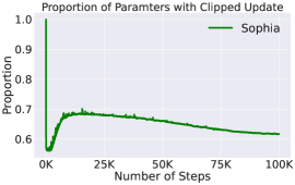
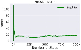
Dynamics of Sophia in training. We measure the norm of the EMA of the diagonal Hessian , and the proportion of parameters where clipping happens (that is, is larger than 1) during pre-training in Figure 9. After the initial stage, the norm of the Hessian steadily grows. The proportion of parameters where clipping happens approaches 60, which corroborates the importance of per-coordinate clipping in the algorithm. We also note that the clipping proportion generally should be between 50% and 90% for Sophia to be effective, and the users are recommended to tune to achieve some a clipping proportion (See Section 3.1 for details).
Results with different number of steps. Runs with different number of steps and their comparison are provided in Figure 10. Across different choices of the total number of steps, Sophia outperforms AdamW and Lion with a large margin as the main experiments we presented in Section 3.3.
Appendix B Additional Experiment Details
B.1 Hyperparamter Tuning
The hyperparameters we consider for baselines are as follows: peak learning rate, , and weight decay. All hyperparameters except the peak learning rate are tuned with grid search on a 30M GPT-2 trained for 50K steps. The peak learning rate is tuned on models of different sizes with grid search separately. We search in and in . Weight decay is chosen from . For Lion, we also include as suggested by Chen et al. (2023). On 30M models, we found AdamW is sensitive to the choice of but not . works the best for AdamW while works the best for Lion. We use for AdamW since this is the dominantly used configuration in the LLM pre-training literature, and for Lion as it is recommended by Chen et al. (2023). We found that weight decay 0.1 works the best for AdamW, while 0.2 works the best for Lion and Sophia.
For peak learning rate on 125M and 355M, we perform a grid search. For larger models, we search for the largest possible learning rate with which training does not blow up for each model in the following list: [6e-4, 4e-4, 3e-4, 2e-4, 1.5e-4, 1.2e-4, 1e-4, 8e-5, 6e-5, 4e-5]. For example, a 6.6B GPT NeoX model work with 1.2e-4 peak learning rate, but the loss will blow up if we increase the learning rate to 1.5e-4 as shown in Figure 12. The result of grid search of peak learning rate is provided in Table 2.
We use , , 1e-12 and for Sophia. We adopt the following procedure to obtain these hyper parameters. We first fix , , and tune and with grid search on a 30M model, and directly use and from the 30M model on models of larger sizes. Similar to AdamW, we find that Sophia is not sensitive to . We then fix , and tuning . As shown in in Figure 8 (a), is better than or in terms of the balance between convergence speed and the computation overhead.
After finding out , , and with the method above, we tune and peak learning rate jointly. We first tune to make the proportion of coordinates where the update is not clipped (i.e., ) in the range of . We search for in the list of [0.005,0.01,0.02,0.05,0.1,0.2]. As a result we find out works the best for Sophia-H while works the best for Sophia-G. We then fix for all larger models.
To tune the peak learning rate, we adopt the same procedure as we use for baseline methods. The result of grid search of peak learning rate is also provided in Table 2.
| Acronym | Size | dmodel | nhead | depth | AdamW lr | Lion lr | Sophia-H lr | Sophia-G lr |
|---|---|---|---|---|---|---|---|---|
| – | 30M | 384 | 6 | 6 | 1.2e-3 | 4e-4 | 1e-3 | 1e-3 |
| Small | 125M | 768 | 12 | 12 | 6e-4 | 1.5e-4 | 6e-4 | 6e-4 |
| Medium | 355M | 1024 | 16 | 24 | 3e-4 | 6e-5 | 4e-4 | 4e-4 |
| – | 540M | 1152 | 18 | 30 | 3e-4 | – | 4e-4 | 4e-4 |
| Large | 770M | 1280 | 20 | 36 | 2e-4 | – | 3e-4 | 3e-4 |
| NeoX 1.5B | 1.5B | 1536 | 24 | 48 | 1.5e-4 | – | – | 1.2e-4 |
| NeoX 6.6B | 6.6B | 4096 | 32 | 32 | 1.2e-4 | – | – | 6e-5 |
B.2 Model and Implementation Details
We consider three sizes of GPT-2 corresponding to small, medium, and large in Radford et al. (2019). We also introduce a 30M model for efficient hyperparameter grid search and a 540M model for scaling law visualization. We provide the model specifications in Table 2. We use the nanoGPT (https://github.com/karpathy/nanoGPT/) code base. Following nanoGPT, we use GELU activations and disable bias and Dropout Srivastava et al. (2014) during pre-training.
GPT-2 models are trained on OpenWebText (Gokaslan & Cohen, 2019). The text is tokenized with the GPT-2 tokenizer (Radford et al., 2019). We use the train and validation split from nanoGPT. The training set contains 9B tokens, and the validation set contains 4.4M tokens.
We use distributed data parallel with gradient accumulation to enable a batch size of 480. All models are trained with bfloat16. The 125M and 355M models are trained on machines with 10 A5000 GPUs, while the 770M models are trained on an AWS p4d.24xlarge instance with 8 A100 GPUs.
We consider 1.5B and 6.6B GPT NeoX (Black et al., 2022) models trained on the Pile (Gao et al., 2020). The models use GPT NeoX tokenizers. We use levanter (https://github.com/stanford-crfm/levanter/tree/main) for GPT NeoX. We use fully sharded data parallel with gradient accumulation to enable a batch size of 512 for the 1.5B model and 1024 for the 6.6B model. These models are trained on a TPU v3-128 slice.
We observed AdamW and Lion does not perform well on standard transformers which are larger than 355M. The iterates become unstable when the learning rate is close to the choice of Radford et al. (2019). We introduce scaling attention by the inverse of layer index to address this issue following Karamcheti et al. (2021); Wolf et al. (2020). Note that Sophia does not need this trick as mentioned in Section 3.4.
B.3 Downtream Evaluation
We perform few-shot evaluation of the models on 4 subtasks of SuperGLUE. We use 2-shot prompting and greedy decoding. The prompt consists of an instruction followed by two examples. The examples are sampled from the train split while we report the accuracy on validation split averaged over 5 selection of exemplars. Prompts for each subtask are illustrated in Figure 11.

Appendix C Limitations
Scaling up to larger models and datasets. Although Sophia demonstrates scalability up to 6.6B-parameter models, and there is no essential constraints from further scaling up, we do not compare with AdamW and Lion on larger models due to limited resources. We believe Sophia is faster than AdamW and Lion on larger models given the improvement in scaling laws and better pre-training stability.
Holistic downstream evaluation. We evaluate pre-trained checkpoints on the pre-training validation losses and only four SuperGLUE subtasks. The limited evaluation in downstream evaluation is partly due to the limited model size, because language models at this scale do not have enough capabilities such as in-context learning, and mathematical reasoning.
Evaluation on other domains. While this paper focuses on optimizers for large language modeling, a more general optimizer should also be evaluated in other domains such as computer vision, reinforcement learning, and multimodal tasks. Due to the limitation of computation resources, we leave the application to other domains and models to future works.
Appendix D Theoretical Analyses: Details of Section 4
Theorem 4.3 is a direct combination of the Lemma D.10 (Descent Lemma), Lemma D.9 and Lemma D.11. In the analysis, there will be two phases. In the first phase decrease loss to in steps. In the second phase, there will be an exponential decay of error.
Lemma D.1.
Under 4.1, we have that whenever .
Proof of Lemma D.1.
By convexity of , we have with ,
| (17) |
Since is strictly convex, . Thus we conclude that
| (18) |
Therefore when , as well. ∎
Note that we don’t assume the Hessian of loss is Lipschitz. 4.2 only assumes the Hessian in a neighborhood of constant radius only differs by a constant in the multiplicative sense.
Lemma D.2.
For any satisfying , it holds that .
Proof of Lemma D.2.
We will prove by contradiction. Suppose there exists such with but . We consider . Since is between and and that is strictly convex, we know that . However, by Taylor expansion on function , we have that
| (19) |
Note that , by 4.2 and 4.1, we have . Also note that and , we conclude that , namely . Contradiction! ∎
Lemma D.3.
For any satisfying that , it holds that .
Proof of Lemma D.3.
Lemma D.4.
For any , the following differential equation has at least one solution on interval :
| (20) |
and the solution satisfies that for all and .
Proof of Lemma D.4.
Since is continuous and positive definite by 4.1 , is continuous and thus the above ODE (45) has a solution over interval for some positive and we let be the largest positive number such that the solution exists (or ). Now we claim , otherwise must diverge to infinity when . However, for any , we have
| (21) |
which implies that for all . Therefore,
| (22) |
Thus . By Lemma D.1, we know that remains bounded for all , thus . Note that has zero gradient, must be . This completes the proof. ∎
Lemma D.5.
For any satisfying (1) or (2) , it holds that
| (23) |
Proof of Lemma D.5.
Let be the solution of Equation 45. We know that for all and that by Lemma D.4. For case (1), by Lemma D.2, we know that for any , . For case (2), by Lemma D.3, we know that for any , . Thus in both two cases, . By 4.2, it holds that
| (24) |
for all . Therefore, we have that
| (25) |
The proof is completed by plugging Equation 24 into Appendix D and noting that . ∎
Lemma D.6.
For any satisfying (1) or (2) , it holds that
| (26) |
Proof of Lemma D.6.
Lemma D.7.
For any satisfying , it holds that
| (27) |
Proof of Lemma D.7.
Lemma D.8.
For any satisfying that , it holds that
| (31) |
Proof of Lemma D.8.
Let be the solution of Equation 45 and we claim that for all , . Otherwise, let be the smallest positive number such that . Such exists because is continuous in and . We have that
| (32) | ||||
| (33) | ||||
| (34) | ||||
| (35) | ||||
| (36) |
which implies . Here in Equation 35, we use 4.2. Thus we conclude that for all , . By 4.2, it holds that
| (37) |
Therefore, we have that
| (38) |
The proof is completed by plugging Equation 37 into Appendix D and noting that . ∎
Lemma D.9.
If , then for any and any satisfying
| (39) |
where is the eigendecomposition of , is the th row of and , it holds that
| (40) |
In particular, if we set , we have .
Proof of Lemma D.9.
Let be the set of indices where clipping does not happen. Then we have that
| (41) | |||
| (42) |
Now we consider a new strictly convex loss function in , which is restricted on the space of , that is, . This new loss function clearly satisfy 4.2 since it is a restriction of into some subspace of . By Lemma D.1, we know that can be attained and we denote it by . By 4.1, we know that is strictly convex and thus , which means 4.1 also holds for .
Next we will apply Lemma D.8 on at . We use to denote the submatrix of containing rows in for any . One can verify by chain rule that and that . Thus we have that
| (43) |
By the definition of , we know that . Thus . Thus we can apply Lemma D.8 on at and conclude that
| (44) |
Thus .
It remains to show that . To do so, our strategy is to first show that is small and then to use Lemma D.6. We will use to denote the complement of in and to denote the submatrix of which contains all the rows that do not belong to . Note that is the minimizer of , we know that and that .
Now we consider the following ODE
| (45) |
By Lemma D.4, we know this ODE has solution over interval with . With the same argument in the proof of Lemma D.8, we know that for all . Thus we have for any ,
| (46) | ||||
| (47) | ||||
| (48) | ||||
| (49) | ||||
| (50) |
For the first term (Equation 49), by 4.2, we have that
| (51) |
For the second term (Equation 50), by 4.2, we have that
| (52) | ||||
| (53) | ||||
| (54) | ||||
| (55) |
Thus we conclude that , which implies that
| (56) | ||||
| (57) | ||||
| (58) | ||||
| (59) |
Lemma D.10 (Descent Lemma).
For any with , and any eigendecomposition of , where , is diagonal , define
| (61) |
it holds that
| (62) |
where is the th row of matrix .
Proof of Lemma D.10.
Let . By the definition of clip operation, we know that . Thus we have . Define . By Assumption 4.2, we know that for all and thus
| (63) |
It remains to show that
-
1.
;
-
2.
;
First, by chain rule, we have .
Second, again by chain rule, we have . Note that by definition , we have , which completes the proof.
∎
Lemma D.11.
If and for some , , then if holds that for all ,
-
1.
;
-
2.
.
Proof of Lemma D.11.
First by Lemma D.10, we have for all , , therefore by Lemma D.7, we have for all , which implies clipping will not happen. This completes the proof of the first claim.
For the second claim, by Lemmas D.10 and D.5, we have that
| (64) | ||||
| (65) | ||||
| (66) |
which completes the proof. ∎
D.1 Lower bound for SignGD on 2-dimensional quadratic loss
Define as a quadratic function with parameter as . We have the following lower bound, which shows signGD’s convergence rate has to depend on the condition number .
Theorem D.12.
For any , suppose there exist a learning rate and a time such that for all satisfying that , signGD reaches loss at most at step and (in the sense that and ). Then, must satisfy .
Proof of Theorem D.12.
We consider two initialization: and , and let and be the iterates under the two initializations. For each coordinate , because , we have that . Thus , which implies .
The fact that implies . Because SignGD can only move each coordinate by at most, we have . Using the fact that , we have that , which completes the proof. ∎