Diffusion Hyperfeatures: Searching Through Time and Space for Semantic Correspondence

Abstract

Diffusion models have been shown to be capable of generating high-quality images, suggesting that they could contain meaningful internal representations. Unfortunately, the feature maps that encode a diffusion model’s internal information are spread not only over layers of the network, but also over diffusion timesteps, making it challenging to extract useful descriptors. We propose Diffusion Hyperfeatures, a framework for consolidating multi-scale and multi-timestep feature maps into per-pixel feature descriptors that can be used for downstream tasks. These descriptors can be extracted for both synthetic and real images using the generation and inversion processes. We evaluate the utility of our Diffusion Hyperfeatures on the task of semantic keypoint correspondence: our method achieves superior performance on the SPair-71k real image benchmark. We also demonstrate that our method is flexible and transferable: our feature aggregation network trained on the inversion features of real image pairs can be used on the generation features of synthetic image pairs with unseen objects and compositions. Our code is available at https://diffusion-hyperfeatures.github.io.

1 Introduction

Much of the recent progress in computer vision has been facilitated by representations learned by deep models. Features from ConvNets [45, 5, 35, 33], Vision Transformers [8, 2], and GANs [38, 23] have demonstrated great utility in a number of applications, even when compared to hand-crafted feature descriptors [21, 6]. Recently, diffusion models have shown impressive results for image generation, suggesting that they too contain rich internal representations that can be used for downstream tasks. Existing works that use features from a diffusion model typically select a particular subset of layers and timesteps that best model the properties needed for a given task (e.g., features for semantic-level correspondence may be most prevalent in middle layers, whereas textural content may be at later layers). This selection not only requires a laborious discovery process hand-crafted for a specific task, but it also leaves behind potentially valuable information distributed across other features in the diffusion process.

In this work, we propose a framework for consolidating all intermediate feature maps from the diffusion process, which vary both over scale and time, into a single per-pixel descriptor which we dub Diffusion Hyperfeatures. In practice, this consolidation happens through a feature aggregation network that takes as input the collection of intermediate feature maps from the diffusion process and produces as output a single descriptor map. This aggregation network is interpretable, as it learns mixing weights to identify the most meaningful features for a given task (e.g., semantic correspondence). Extracting Diffusion Hyperfeatures for a given image is as simple as performing the diffusion process for that image (the generation process for synthetic images, and inversion for real images) and feeding all the intermediate features to our aggregator network.

We evaluate this approach by training and testing our descriptors on the task of semantic keypoint correspondence, using real images from the SPair-71k benchmark [25]. We present an analysis of the utility of different layers and timesteps of diffusion model features. Finally, we evaluate our trained feature aggregator on synthetic images generated by the diffusion model and show that our Diffusion Hyperfeatures generalize to out-of-domain data.

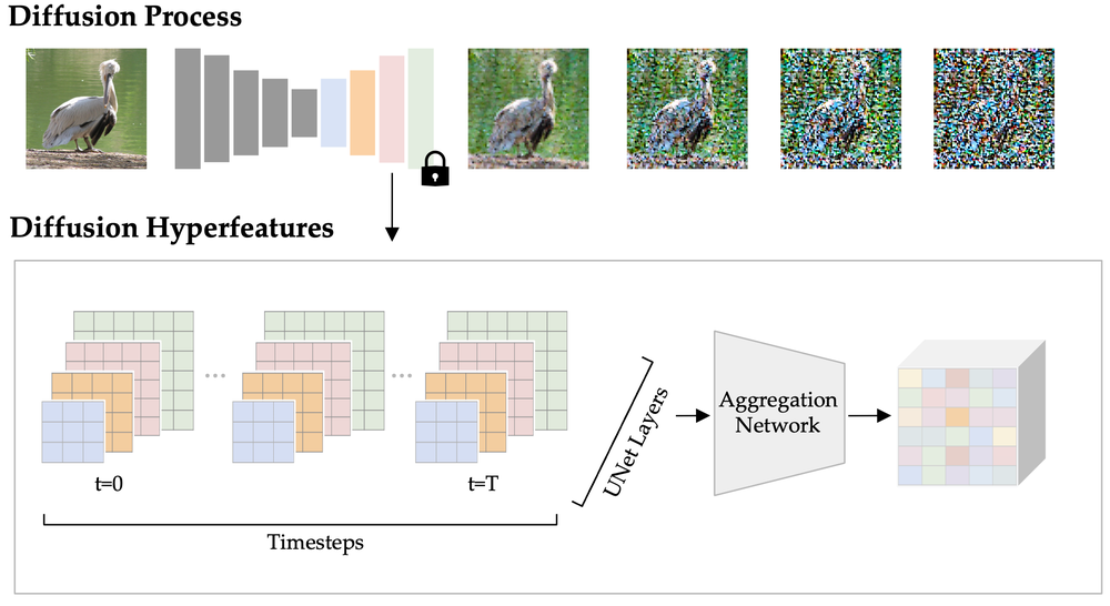
Figure 1: Unlike prior work that hand-selects a subset of raw diffusion features, we extract all feature maps from the diffusion process, varying across both timesteps and layers, and use a lightweight aggregation network to consolidate them into Diffusion Hyperfeatures. For real images, we extract these features from the inversion process, and for synthetic images we extract these features from the generation process. Given a pair of images, we find semantic correspondences by performing a nearest-neighbor search over their Diffusion Hyperfeatures.

2 Related Work

Hypercolumn Features. The term hypercolumn, originally from neuroscience literature [15], was first coined for neural network features by Hariharan et al. [12] to refer to the set of activations corresponding to a pixel across layers of a convolutional network, an idea that has also been studied in the context of texture [22], optical flow [39], and stereo [17]. One central idea of this line of work is that for precise localization tasks such as keypoint detection and segmentation [12, 43], it is essential to reason at both coarse and fine scales rather than the typical coarse-to-fine setting. The usage of hypercolumns has also been popular for the task of semantic correspondence, where approaches must be coarse enough to be robust to illumination and viewpoint changes and fine enough to compute precise matches [24, 27, 37, 26, 1]. Our work revisits the idea of hypercolumns to leverage the features of a recently popular network architecture, diffusion models, which primarily differ from prior work in that the underlying feature extractor is trained on a generative objective and offers feature variation along the axis of time in addition to scale.

Deep Features for Semantic Correspondence. There has been a recent interest in transferring representations learned by large-scale models for the task of semantic correspondence. Peebles et al. [29] addressed the task of congealing [20] by supervising a warping network with synthetic GAN data produced from a learned style vector representing shared image structure. While prior work [29, 36] has demonstrated that generative models can produce aligned image outputs, which is useful supervision for semantic correspondence, we study how well the raw intermediate representations themselves would perform for the same task. Utilizing self-supervised representations, in particular from DINO [4], has also been especially popular. Prior work has demonstrated that it is possible to extract high-quality descriptors from DINO that are robust and versatile across domains and challenging instances of semantic correspondence [2]. These descriptors have been used for downstream tasks such as semantic segmentation [11], relative camera pose estimation [9], and dense visual alignment [28, 10]. While DINO does indeed contain a rich visual representation, diffusion features are under-explored for the task of semantic correspondence and likely contain enhanced semantic representations due to training on image-text pairs.

Diffusion Model Representations. There have been a few works that have analyzed the underlying representations in diffusion models and proposed using them for downstream tasks. Plug-and-Play [36] injects intermediate features from a single layer of the diffusion UNet during a second generation process to preserve image structure in text-guided editing. FeatureNeRF [42] distills diffusion features from this same layer into a neural radiance field. DDPMSeg [3] and ODISE [41] aggregate features from a hand-selected subset of layers and timesteps for semantic and panoptic segmentation respectively. While these works also consider a subset of features across layers and/or time, our work primarily differs in the following ways: first, rather than hand-selecting a subset of features, we propose a learned feature aggregator building on top of Xu et al. [41] that weights all features and distills them into a concise descriptor map of a fixed channel size and resolution. Furthermore, all of these methods solely use the generation process to extract representations, even for real images. In contrast, we use the inversion process, where we are able to extract higher-quality features at these same timesteps, as seen in Figure 3.

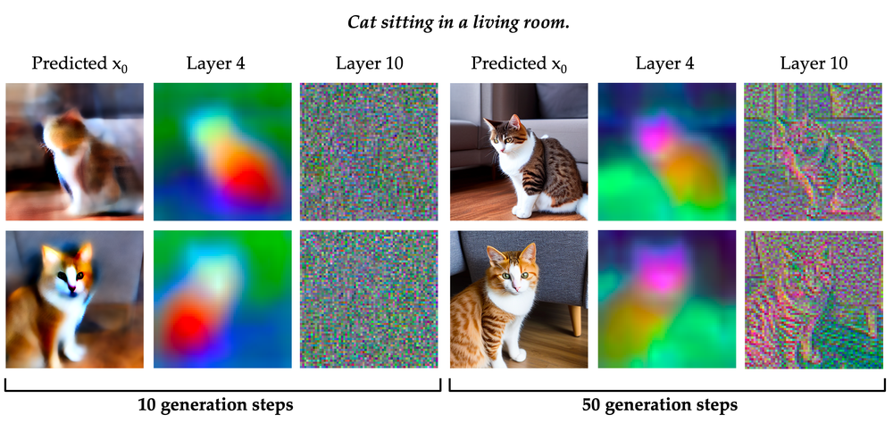
Figure 2: We show an example pair of synthetic images for the prompt “cat sitting in a living room” and the PCA of the features from Layers 4, 10 during both an early and late generation step. While different layers capture different image characteristics (here Layer 4 delineates the face vs. body and Layer 10 captures the edges), these features also evolve and become more fine-grained over time.

3 Diffusion Hyperfeatures

In a diffusion process, one makes multiple calls to a UNet to progressively noise the image (in the case of inversion) or denoise the image (in the case of generation). In either case, the UNet produces a number of intermediate feature maps, which can be cached across all steps of the diffusion process to amass a set of feature maps that vary over timestep and layers of the network. This feature set is rather large and unwieldy, varying in resolution and detail across different axes, but contains rich information about texture and semantics. We propose using a lightweight aggregation network to learn the relative importance of each feature map for a given task (in this paper we choose semantic correspondence) and consolidate them into a single descriptor map (our Diffusion Hyperfeatures). To assess the quality of this descriptor map, we compute semantic correspondences for an image pair, by using a nearest-neighbors search on the extracted descriptors, and compare these correspondences to the ground-truth annotations [25, 40]. An overview of our method is shown in Figure 1.

Our approach is composed of two core components. Extraction (Section 3.1): We formulate a simplified and unified extraction process that accounts for both synthetic and real images, which means we are able to use the same aggregation network on features from both image types. Aggregation (Section 3.2): We propose an interpretable aggregation network that learns mixing weights across the features, which highlights the layers and timesteps that provide the most useful features unique to the underlying model and task.

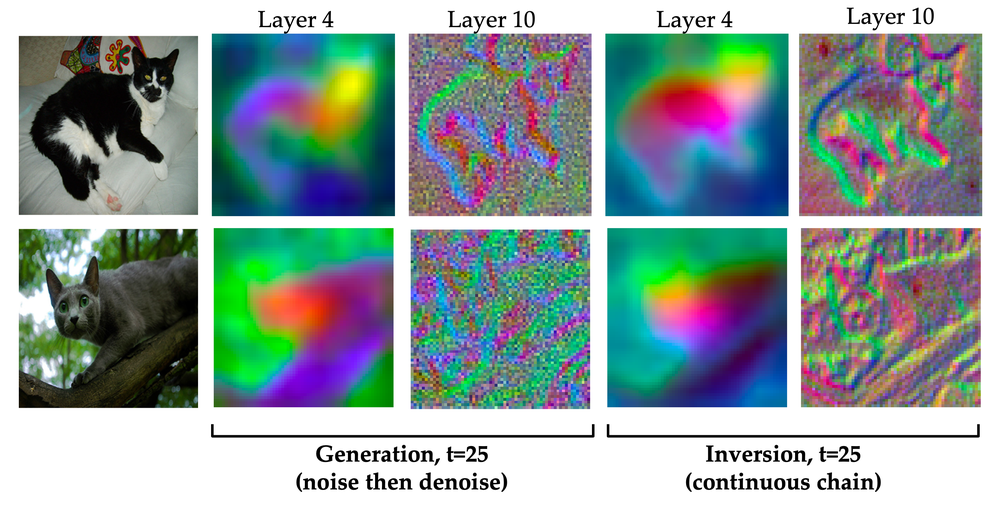
Figure 3: We show an example pair of real images from SPair-71k and the PCA of the features from Layers 4, 10 when extracted at the middle timestep $t=25$. While prior work extracts generation features by noising and denoising the image independently at the specific timestep (left), in our approach we extract inversion features from one continuous chain (right). Extracting features from the same timestep of the inversion chain can produce features more true to original image content.

3.1 Diffusion Process Extraction

One popular sampling procedure for a trained diffusion model is DDIM sampling [34] of the form

$$x_{t}=\sqrt{\alpha_{t}}x_{0}+\sqrt{1-\alpha_{t}}\epsilon_{t}\textrm{ where }\epsilon_{t}\sim\mathcal{N}(0,1)$$

where $x_{0}$ is the clean image, $\epsilon_{t}$ is the noise prediction from the diffusion model conditioned on the timestep $t$ and noisy image $x_{t+1}$ from the previous timestep, and $x_{t}$ is the prediction for the next timestep. To run generation, one runs the reverse process from $t=T$ to $0$, with the input $x_{T}$ set to pure noise sampled from $\mathcal{N}(0,1)$. To run inversion, one runs the forward process from $t=0$ to $T$, with the input $x_{0}$ set to the clean image.
Generation. When synthesizing an image, we can cache the intermediate feature maps across the generation process, which already contain shared representations that can be used to relate the image to other synthetic images, as seen in the PCA visualization of the feature maps in Figure 2. In this example, we see that the head and body of the two cats share a corresponding latent representation throughout almost the entire generation process, even as early as the first ten steps, where the inputs to the UNet are almost pure noise. This can be explained by the preliminary prediction for the final image $x_{0}$, which already lays out the general idea of the image including the structure, color, and main subject. As generation progresses, the principal components of the features also evolve, with Layer 4 changing from displaying coarse to more refined common semantic sub-parts and Layer 10 changing from displaying no shared characteristics to high-frequency image gradients. These observations indicate that the diffusion model provides coarse and fine features that capture different image characteristics (i.e. semantic or textural information) throughout different combinations of layers and timesteps. Hence, we find it important to extract features from all layers and timesteps in order to adequately tune our final descriptor map to represent the appropriate level of granularity needed for a given task.
Inversion. These same useful features can be extracted for real images through the inversion process. Although inversion is a process that destructs the real image into noise, we observe that its features contain useful information akin to the generation process for synthetic images. In Figure 3, we can see that our inversion features are able to reliably capture the full body of both cats and their common semantic subparts (head, torso, legs) in Layer 4 and their edges in Layer 10 even at a timestep when the input to the model is relatively noisy. In contrast, using the generation process to analyze real images (as done in prior work) leads to hyperparameter tuning and tradeoffs. For example, at timesteps close to $t=T$ where in-distribution inputs are close to noise, the features start to diverge from information present in the real image and may even hallucinate extraneous details, as seen in Figure 3. In this example, because the color of the top cat’s stomach is white like the background, the generation features from Layer 4 merge the stomach with the background. Similarly, because there is low contrast between the bottom cat and the background, the generation features from Layer 10 fail to capture the silhouette of the cat and instead depict random texture edges. Intuitively, inversion features are more trustworthy because of the notion of chaining, where at every step the input is some previous output of the model rather than a random mixture of an image and noise, and every extracted feature map is therefore interrelated. Extracting features from a continuous inversion process is also nice because it induces symmetry with the generation process, which in Section 4.3 we demonstrate allows us to use both feature types interchangeably with the same aggregation network.

3.2 Diffusion Hyperfeatures Aggregation

Given a dense set of feature maps from the diffusion process, we now must efficiently aggregate them into a single descriptor map without omitting the information from any layers or timesteps. A naive solution would be to simply concatenate all feature maps into one very deep feature map, but this proves to be too high dimensional for most applications. We address this issue with our aggregation network, which standardizes the feature maps with tuned bottleneck layers and sums them according to learned mixing weights. Specifically, for a given feature map $r$ we upsample it to a standard resolution, pass through a bottleneck layer $B$ [13, 41] to a standard channel count, and weight it with a mixing weight $w$. The final Diffusion Hyperfeatures take on the form

$$\sum_{s=0}^{S}\sum_{l=1}^{L}w_{l,s}\cdot B_{l}(r_{l,s})$$

where $L$ is the total number of layers and $S$ is the total number of timesteps. Note that we run the diffusion process for a total number of $T$ timesteps but only select a subsample of $S$ timesteps for aggregation to conserve memory. We opt to share bottleneck layers across timesteps, meaning we use a total of $L$ bottleneck layers. However, we learn $L\cdot S$ unique mixing weights for every combination of layer and timestep. We then tune these bottleneck layers and mixing weights using task-specific supervision. For semantic correspondence, we flatten the descriptor maps for a pair of images and compute the cosine similarity between every possible pair of points. We then supervise with the labeled corresponding keypoints using a symmetric cross entropy loss in the same fashion as CLIP [30]. During training, we downscale the labels according to the resolution of our descriptor maps. When running inference, we upsample the descriptor maps before performing nearest neighbors matching to predict semantic keypoints. We demonstrate that this lightweight parameterization of our aggregation network is performant (see Section 4.1) and interpretable (see Section 4.2) without degrading the open-domain knowledge represented in the diffusion features (see Section 4.3).

4 Experiments

Baselines. We compare against descriptors derived from DINO [4], a self-supervised model trained on ImageNet [7]. Specifically, we compare against the method from Amir et al. [2], which extracts key features from specific DINO ViT layers. We also compare against hypercolumn features from DHPF [26], a supervised model for semantic correspondence trained on SPair-71k [25]. The method composes features across relevant layers of a ResNet-101 [13] backbone. Our method extracts descriptors from Stable Diffusion v1-5 [31], a generative latent diffusion model trained on LAION-5B [32]. We extract Diffusion Hyperfeatures aggregated from features across UNet layers and timesteps. We tune our bottleneck layers and mixing weights on SPair-71k for up to 5000 steps with a learning rate of 1e-3 and Adam optimizer [18]. This means that we tune on at most 5k out of the 53k possible training samples, where we find that training on additional samples does not further improve performance.
Experimental Details. We extract features from the UNet decoder layers (denoted as Layers 1 to 12), specifically the outputs of the residual block before the self- and cross- attention blocks. When running either the inversion or generation process we use $T=50$ scheduler timesteps, except when we denote that the process is “one-step” ($T=1$). We subsample every $5$ timesteps when aggregating features across time to conserve memory.
Metrics. We report results in terms of PCK@$\alpha$, or the percentage of correct keypoints at the threshold $\alpha$. The predicted keypoint is considered to be correct if it lies within a radius of $\alpha*max(h,w)$ of the ground truth annotation, where $h,w$ denotes the dimensions of the entire image ($\alpha_{img}$) or object bounding box ($\alpha_{bbox}$) in the original image resolution. Following Amir et al. [2] we use the threshold $\alpha=0.1$ [2].

4.1 Semantic Keypoint Matching on Real Images

			SPair-71k		CUB
	# Layers	# Timesteps	$\uparrow$ PCK@$0.1_{\text{img}}$	$\uparrow$ PCK@$0.1_{\text{bbox}}$	$\uparrow$ PCK@$0.1_{\text{img}}$	$\uparrow$ PCK@$0.1_{\text{bbox}}$
DINO [2]	1	-	51.68	41.04	72.72	55.90
DHPF [26]	34	-	55.28	42.63	77.30	61.42
SD-Layer-4	1	1	58.80	46.58	78.43	61.22
SD-Concat-All	12	1	52.12	41.83	70.22	54.05
Ours	12	11	72.56	64.61	82.29	69.42
Ours-One-Step	12	1	63.74	54.69	76.59	62.11
SD-Layer-Pruned	1	1	57.69	48.16	80.67	67.21
Ours-Pruned	1	1	64.02	53.74	79.10	63.95
Ours-SDv2-1	12	11	70.74	64.85	80.39	68.04

Table 1: We evaluate our semantic keypoint matching performance on real images from SPair-71k and CUB. For our CUB evaluation, we transfer the model tuned on Spair-71k. For our Stable Diffusion baselines, we extract features from a single layer (SD-Layer-4) or concatenation of all layers (SD-Concat-All) from a one-step inversion process, selecting features from $S=1$ timesteps. Otherwise we run a fifty-step inversion process and aggregate features from $S=11$ timesteps. We ablate pruning to the single feature map with the highest mixing weight selected by our method, either as the raw feature map (SD-Layer-Pruned) or after the bottleneck layer (Ours-Pruned). We also ablate tuning our method with only one timestep (One-Step) or features from another Stable Diffusion variant (SDv2-1). Otherwise we extract features from SDv1-5.

We evaluate on the semantic keypoint correspondence benchmark SPair-71k [25], which is composed of image pairs from 18 object categories spanning animals, vehicles, and household objects. Following prior work [2], we evaluate on 360 random image pairs from the test split, with 20 pairs per category. We also evaluate on CUB [40], which is composed of semantic keypoints on a variety of bird species. We evaluate on 360 random image pairs from the validation split used by Kulkarni et al. [19]. The CUB dataset is completely unseen to all methods, meaning that we only tune with SPair-71k and evaluate transferring the same model onto CUB.

We evaluate our method in Table 1, comparing against DINO descriptors [2] and task-specific hypercolumns [26]. We also compare against two Stable Diffusion baselines, selecting a single feature map from a known semantic layer [36] (SD-Layer-4) and concatenating feature maps from all layers (SD-Concat-All). For our diffusion baselines we perform one-step inversion, meaning we collapse the time dimension by setting the total number of scheduler timesteps to 1. Selecting a single diffusion feature map (SD-Layer-4) already outperforms DINO and DHPF by a margin of at least 4% in PCK@$0.1_{\text{img}}$ , likely due to the underlying model’s larger and more diverse training set. Conversely, naively concatenating all feature maps (SD-Concat-All), degrades this improvement, likely because each map captures a different level of granularity and therefore should not be equally weighted for a coarse-level semantic similarity task. When aggregating all feature maps across time and space using our Diffusion Hyperfeatures, we see a significant boost of 14% in PCK@$0.1_{\text{img}}$ . This sizeable performance improvement indicates that (1) while a single layer may capture a good deal of semantic information, the other layers also capture complementary information that can be useful for disambiguating points on a finer level and (2) the diffusion model’s internal knowledge about the image is not fully captured by a single pass through the UNet but is rather spread out over multiple timesteps.

In Figure 4, we show qualitative examples of our predicted semantic correspondences compared with DINO and SD-Layer-4. In general, while both baselines are able to relate broad semantic regions such as the head, arms, or legs, they struggle with fine-grained subparts and confuse them with other visually similar regions. For example, SD-Layer-4 confuses the headlight (yellow) of the blue car with the rear light of the red car, whereas our method is able to correctly reason about the front vs. back of the cars. DINO confuses the nose (blue) and tail (cyan) of the miniature pinscher dog with the ears and knee of the greyhound, whereas our method finely localizes these subparts. Both baselines confuse the the tail (cyan) of the seagull with the beak of the northern flicker bird, likely because both are distinctive corners, whereas our method is able to correctly place the tail and beak (yellow) on opposite sides.

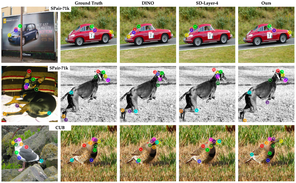
Figure 4: Example images from SPair-71k and CUB, the ground-truth user-annotated correspondences, and predicted correspondences from DINO, SD-Layer-4, and our method.

4.2 Ablations

Number of Diffusion Steps. We ablate the importance of the time dimension by tuning a variant of our method on feature maps from a one-step inversion process (Ours-One-Step), where there is only one possible timestep to extract from. While this variant that aggregates over all layers performs better than single layer selection (SD-Layer-4) or simple concatenation (SD-Concat-All) by a margin of at least 5% in PCK@$0.1_{\text{img}}$ , it also heavily lags behind our full method. As indicated by our mixing weights in Figure 5, the most useful information for semantic correspondence are concentrated in the early timesteps of the diffusion process, where the input image is relatively clean but contains some noise. Timestep selection can be thought of as a knob for the amount of high frequency detail present in the image to analyze, where at these early timesteps the model is implicitly mapping the noisy input to a smoother image, similar to the oversmoothed cats for the predicted $x_{0}$ in Figure 2. Evidently not all texture and detail is necessary for the task of semantic correspondence, and the model is able to produce more useful features at different timesteps which highlight different image frequencies.

Pruning. Since our method employs interpretable mixing weights, we have a ranking of the relative importance of each layer and timestep combination for the task of semantic correspondence. To verify this ranking, we ablate pruning to the single feature map with the highest mixing weight. As seen in Figure 5, for Ours-SDv1-5 this is the feature map associated with Layer 5, Timestep 10. Referring to Table 1, this automatically selected raw feature map (SD-Layer-Pruned) performs comparably to the feature map manually selected by prior work (SD-Layer-4). Interestingly, if only viewing features from a one-step inversion process it would seem that Layer 5 features are significantly worse than Layer 4 features, as discussed further in the Supplemental, but the story changes after tuning selection over both time and space. After passing this pruned feature map to our learned bottleneck layer, the feature map performs comparably on CUB and 6% better in PCK@$0.1_{\text{img}}$ on SPair-71k, as seen when comparing SD-Layer-Pruned and Ours-Pruned in Table 1. This trend validates that our bottleneck layer does not degrade the power of the original representation, but rather refines it in a way that is likely helpful for complex object categories present in SPair-71k beyond birds. Considering the 9% gap in PCK@$0.1_{\text{img}}$ between our pruned and full method (Ours-Pruned vs. Ours), it becomes evident that it is not a single feature map that drives our strong performance but rather the soft mixing of many feature maps.

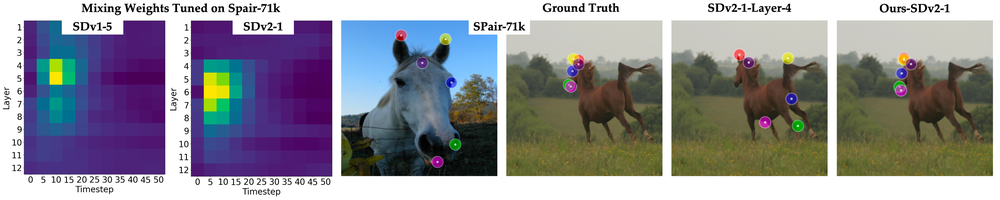
Figure 5: The learned mixing weights for the variant of our method that aggregates SDv1-5 vs. SDv2-1 features across multiple layers and timesteps. Bright yellow denotes a high weighting, and dark blue denotes a low weighting. We also depict an example of predicted correspondences from SDv2-1-Layer-4 and Ours-SDv2-1. While raw features from SDv1-5-Layer-4 perform well in semantic correspondence, these same features of SDv2-1 perform extremely poorly. On the other hand, our method is able to aggregate different feature combinations depending on the model variant.

Model Variant. We also ablate using a different model variant for our diffusion feature extraction, namely SDv2-1. Most notably, SDv2-1 differs from SDv1-5 in its large-scale text encoder, which scales from CLIP [30] to OpenCLIP [16]. The mixing weights learned for both model variants, depicted in Figure 5, showcase the same high-level trends, where the features found to be the most useful for semantic correspondence are concentrated in middle Layers 4-9 and early Timesteps 5-15. However, on a more nuanced level, the behavior starts to diverge with regards to the relative importance of layers and timesteps within this range. Namely, layer selection moves from Layers 4-5 to higher resolution Layers 5-7 from SDv1-5 to v2-1. This behavior is confirmed by our early hyperparameter sweeps of raw feature maps across model variants discussed in the Supplemental, where in fact the Layer 4 feature map of SDv2-1 performs extremely poorly for the task of semantic correspondence. Timestep selection also moves from Timestep 10 to Timestep 5 from SDv1-5 to v2-1, which is surprising because this means that SDv2-1 tends to select higher resolution feature maps from timesteps with higher frequency inputs for a task where it is essential to abstract fine-grained details into semantically meaningful matches. These trends seem to imply that a more powerful text encoder produces shared semantic representations at increased levels of detail, possibly because the model is better able to connect more distantly related visual concepts via text instead of giving them completely disjoint representations. Hence, our aggregation network is able to dynamically adjust to the representations being aggregated and the task at hand, both of which influence the most important set of features to select from the diffusion process.

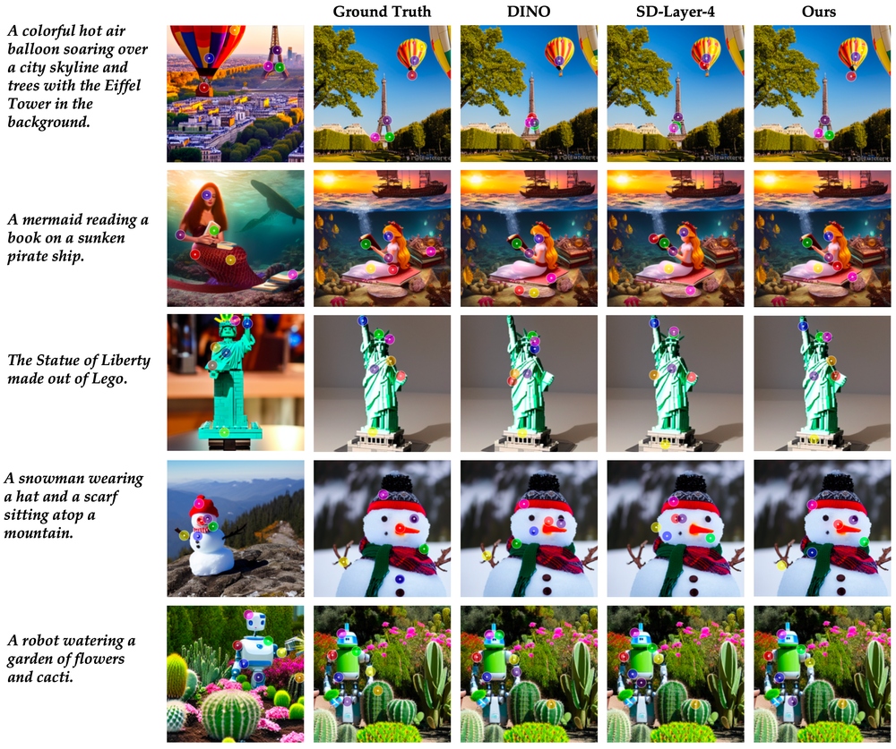
Figure 6: Example synthetic images and their text prompts, the ground-truth user-annotated correspondences, and predicted correspondences from DINO, SD-Layer-4, and our method. Note that we transfer the aggregation network tuned on inversion features of real images, and we apply it on generation features of these synthetic images that are completely out-of-domain compared to the SPair-71k categories.

4.3 Transfer on Synthetic Images

In addition to evaluating the transfer of our aggregation network to other datasets such as CUB, we also evaluate on synthetic images. Specifically, we take the same aggregation network tuned on inversion features and simply flip the timestep ordering to operate on generation features. Therefore in this setting, we are testing our network’s ability to generalize (1) to a completely unseen feature type from a different diffusion process (inversion vs. generation) and (2) out-of-domain object categories that are not present in SPair-71k. Surprisingly, our network generalizes well, outperforming predictions from both DINO and the raw feature map from the last step of the generation process (SD-Layer-4) as seen in Figure 6. Although DINO and SD-Layer-4 are generally able to correspond broad semantic regions correctly, they sometimes have difficulty with relative placement of subparts. In the case of the rungs of the Eiffel Tower (purple, pink, green), DINO collapses all of its predictions onto the middle rung and SD-Layer-4 collapses them onto the left rung, whereas our method is able to correctly correspond the middle and side rungs of the tower in a triangle formation. The baselines can also be distracted by other objects in the scene that are visually similar. In the case of the mermaid’s legs (red, yellow), both baselines incorrectly correspond certain points with the rock in the right image, whose contours and silhouette resemble the legs. On the other hand, our method is able to predict more reliable correspondences for fine-grained subparts, even in these challenging cases with unseen textures (lego, snow) and categories (hat, cactus). The ability of our aggregation network to extend to open-domain synthetic images opens up the exciting possibility of generating custom synthetic datasets with pseudo ground-truth semantic correspondences, which we demonstrate are more precise than correspondences derived from the raw feature maps.

5 Conclusion

We demonstrate that our Diffusion Hyperfeatures are able to distill the information distributed across time and space from a diffusion process into a single descriptor map. Our intepretable aggregation network also enables automatic analysis of the most useful layers and timesteps based on both the underlying model and task of interest. We outperform methods that use supervised hypercolumns or self-supervised descriptors by a large margin on a semantic keypoint correspondence benchmark comprised of real images. Although we tune on a small set of real images with limited categories, we demonstrate that our method is able to retain the open-domain capabilities of the underlying diffusion features by demonstrating strong performance in predicting semantic correspondences in challenging synthetic images, especially compared to using the raw feature maps. Our ability to predict high-quality correspondences derived from the same feature maps used to produce the synthetic image could potentially be employed to create synthetic image sets with pseudo-labeled semantic keypoints, which would be valuable for downstream tasks such as image-to-image translation or 3D reconstruction.

6 Acknowledgements

We thank Angjoo Kanazawa, Yossi Gandelsman, Norman Mu, and David Chan for helpful discussions. This work was supported in part by DoD including DARPA’s SemaFor, PTG and/or LwLL programs, as well as BAIR’s industrial alliance programs.

Supplementary Material

Figure 7: We report the behavior of individual layers across different variants of Stable Diffusion, extracting the raw feature map from a one-step inversion process and computing the semantic keypoint matching performance on real images from SPair-71k. Note that for efficiency reasons in this experiment we compute nearest neighbors matches on 64x64 resolution feature maps and rescale the predictions to the original image resolution.

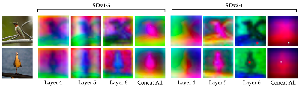
Figure 8: We show an example pair of real images from SPair-71k and the PCA of the features from Layers 4-6 and Concat All extracted from a one-step inversion process for SDv1-5 and SDv2-1.

6.1 Computational Resources

Our final aggregation network takes one day to train on one Nvidia Titan RTX GPU. Inference with our method is fast and uses a reasonable amount of memory, and it can run on a Nvidia T4 GPU on a Google Colab notebook.

6.2 Stable Diffusion Model Variant

In Figure 7, we ablate the behavior of individual raw feature maps from each layer across multiple variants of Stable Diffusion. We extract these features from a one-step inversion process. We report the semantic keypoint matching accuracy on real images from SPair-71k according to PCK@$0.1_{\text{img}}$ . Due to limited computational resources, in this experiment we performed nearest neighbor matching on 64x64 resolution feature maps (the maximum possible resolution of Stable Diffusion) and rescaled our predictions to coordinates in the original image resolution. Therefore, we also include a DINO baseline [2] that uses the same procedure as reference for this experimental setting.

Viewing Figure 7, for Stable Diffusion models that share the same broader model variant (e.g., SDv1-3 vs. SDv1-4 vs. SDv1-5), the behavior across layers is similar. In contrast, there is a larger difference in layer behavior when comparing SDv1 (pink) and SDv2 (blue). For SDv1 Layer 4 outshines all other layers, consistent with observations from prior work [36], but this layer actually performs extremely poorly in SDv2. In fact, for SDv2 it is Layers 5 and 6 that are the layers that are strong at semantic correspondence. As seen in Figure 8, SDv2-1’s Layer 4 features seem to perform poorly at semantic correspondence because they also strongly encode positionality; while they are able to disambiguate the birds and the backgrounds, they also separate the top left (green), top right (blue), bottom left (orange), and bottom right (pink) of the image. Perhaps SDv2 also encodes positionality in the Layer 4 features because this information is relevant when synthesizing images from prompts that describe relations or more complex object compositions, which SDv1’s CLIP struggles with representing [14]. Finally, the behavior when concatenating feature maps from all layers (Concat All) is also very different between SDv1 and SDv2 when viewing Figure 7. While for SDv1 Concat All performs reasonably well, slightly lagging behind its single best feature map, for SDv2 it exhibits subpar performance. This trend is better understood when examining the PCA of these feature maps for two images in Figure 8, where for SDv1-5 Concat All produces a meaningful feature map that delineates the bird, branch, and background and for SDv2-1 Concat All produces a muddy feature map that only delinates the top vs. bottom of the image. This phenomenon where SDv2 produces a low-quality aggregated feature map in the case of simple concatenation is likely also because its stronger encoding of positionality dominates the encoding of semantics across the features. On the other hand, our method is able to meaningfully aggregate features across layers for both SDv1 and SDv2, as demonstrated by the strong keypoint matching performance from both variants in Table 1. Our method is also able to reflect the differing layer behaviors across different Stable Diffusion variants, as seen by the consistency between the the trends observed in Figure 7 and the learned mixing weights in Figure 5.

6.3 Validation Performance

In Table 2 we report our performance compared with DINO [2], DHPF [26], and the Stable Diffusion baselines on 360 image pairs from SPair-71k’s validation split. The trends are similar to our observations in Table 1, where SD-Layer-4 outperforms DINO by 5% PCK@$0.1_{\text{img}}$ and our method outperforms the baselines by at least 15% PCK@$0.1_{\text{img}}$ .

6.4 Additional Examples

In Figure 9, we show additional examples of real image pairs from each of the 18 object categories in SPair-71k and our method’s predicted correspondences. Our method is able to handle a variety of difficult cases such as large viewpoint transformations (e.g., the side and front views of the cow or aeroplane) and occlusions from other objects (e.g., the people on top of the motorbike or bars in front of the potted plant).

In Figure 10, we show additional examples of synthetic image pairs and our method’s predicted correspondences. Many of the prompts were inspired by objects and compositions from PartiPrompts [44]. In the same setting as Section 4.3, we transfer the aggregation network tuned on real images to make these predictions. Our method is able to produce high-quality correspondences for these out-of-domain synthetic images, such as the astronaut riding a horse or raccoon playing chess.

			SPair-71k
	# Layers	# Timesteps	$\uparrow$ PCK@$0.1_{\text{img}}$	$\uparrow$ PCK@$0.1_{\text{bbox}}$
DINO [2]	1	-	53.27	42.91
DHPF [26]	34	-	59.77	45.51
SD-Layer-4	1	1	58.39	46.39
SD-Concat-All	12	1	51.36	41.87
Ours	12	11	74.91	66.08

Table 2: We evaluate our keypoint matching performance on 360 random pairs of real images from SPair-71k’s validation split.

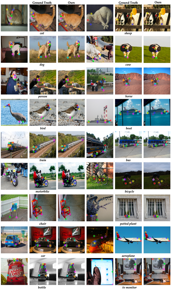
Figure 9: Additional examples of predicted correspondences from our method on real images from each of the 18 categories in SPair-71k.

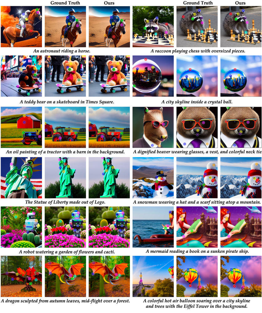
Figure 10: Additional examples of predicted correspondences from our method on synthetic images from a diverse set of prompts. Note that for synthetic images we transfer the aggregation network tuned on real images from SPair-71k.

References

- [1] Kfir Aberman, Jing Liao, Mingyi Shi, Dani Lischinski, Baoquan Chen, and Daniel Cohen-Or. Neural best-buddies: Sparse cross-domain correspondence. ACM Transactions on Graphics (TOG), 37(4):1–14, 2018.
- [2] Shir Amir, Yossi Gandelsman, Shai Bagon, and Tali Dekel. Deep vit features as dense visual descriptors. Proceedings of the European Conference on Computer Vision Workshops (ECCVW), 2022.
- [3] Dmitry Baranchuk, Andrey Voynov, Ivan Rubachev, Valentin Khrulkov, and Artem Babenko. Label-efficient semantic segmentation with diffusion models. In International Conference on Learning Representations, 2022.
- [4] Mathilde Caron, Hugo Touvron, Ishan Misra, Hervé Jégou, Julien Mairal, Piotr Bojanowski, and Armand Joulin. Emerging properties in self-supervised vision transformers. In Proceedings of the International Conference on Computer Vision (ICCV), 2021.
- [5] Qifeng Chen and Vladlen Koltun. Photographic image synthesis with cascaded refinement networks. In Proceedings of the IEEE international conference on computer vision, pages 1511–1520, 2017.
- [6] Navneet Dalal and Bill Triggs. Histograms of oriented gradients for human detection. In 2005 IEEE computer society conference on computer vision and pattern recognition (CVPR’05), volume 1, pages 886–893. Ieee, 2005.
- [7] Jia Deng, Wei Dong, Richard Socher, Li-Jia Li, Kai Li, and Li Fei-Fei. Imagenet: A large-scale hierarchical image database. In 2009 IEEE conference on computer vision and pattern recognition, pages 248–255. Ieee, 2009.
- [8] Alexey Dosovitskiy, Lucas Beyer, Alexander Kolesnikov, Dirk Weissenborn, Xiaohua Zhai, Thomas Unterthiner, Mostafa Dehghani, Matthias Minderer, Georg Heigold, Sylvain Gelly, Jakob Uszkoreit, and Neil Houlsby. An image is worth 16x16 words: Transformers for image recognition at scale. In ICLR, 2021.
- [9] Walter Goodwin, Sagar Vaze, Ioannis Havoutis, and Ingmar Posner. Zero-shot category-level object pose estimation. In Proceedings of the European Conference on Computer Vision (ECCV), 2022.
- [10] Kamal Gupta, Varun Jampani, Carlos Esteves, Abhinav Shrivastava, Ameesh Makadia, Noah Snavely, and Abhishek Kar. Asic: Aligning sparse in-the-wild image collections, 2023.
- [11] Mark Hamilton, Zhoutong Zhang, Bharath Hariharan, Noah Snavely, and William T. Freeman. Unsupervised semantic segmentation by distilling feature correspondences. In International Conference on Learning Representations, 2022.
- [12] Bharath Hariharan, Pablo Arbeláez, Ross Girshick, and Jitendra Malik. Hypercolumns for object segmentation and fine-grained localization. In Proceedings of the IEEE conference on computer vision and pattern recognition, 2015.
- [13] Kaiming He, Xiangyu Zhang, Shaoqing Ren, and Jian Sun. Deep residual learning for image recognition. In Proceedings of the IEEE Conference on Computer Vision and Pattern Recognition (CVPR), 2016.
- [14] Ziqi Huang, Tianxing Wu, Yuming Jiang, Kelvin C.K. Chan, and Ziwei Liu. ReVersion: Diffusion-based relation inversion from images. arXiv preprint arXiv:2303.13495, 2023.
- [15] D. H. Hubel and T. N. Wiesel. Receptive fields, binocular interaction and functional architecture in the cat’s visual cortex. The Journal of Physiology, 160(1), 1962.
- [16] Gabriel Ilharco, Mitchell Wortsman, Ross Wightman, Cade Gordon, Nicholas Carlini, Rohan Taori, Achal Dave, Vaishaal Shankar, Hongseok Namkoong, John Miller, Hannaneh Hajishirzi, Ali Farhadi, and Ludwig Schmidt. Openclip, July 2021. If you use this software, please cite it as below.
- [17] D. G. Jones and J. Malik. Determining three-dimensional shape from orientation and spatial frequency disparities. In European Conference on Computer Vision, 1992.
- [18] Diederik P. Kingma and Jimmy Ba. Adam: A method for stochastic optimization. arXiv preprint arXiv:1412.6980, 2014.
- [19] Nilesh Kulkarni, Abhinav Gupta, David F Fouhey, and Shubham Tulsiani. Articulation-aware canonical surface mapping. In Proceedings of the IEEE/CVF Conference on Computer Vision and Pattern Recognition, pages 452–461, 2020.
- [20] Erik G. Learned-Miller. Data driven image models through continuous joint alignment. IEEE Transactions on Pattern Analysis and Machine Intelligence, 28(2):236–250, 2006.
- [21] David G. Lowe. Distinctive image features from scale-invariant keypoints. Int. J. Comput. Vision, 60(2):91–110, nov 2004.
- [22] J. Malik and P. Perona. Preattentive texture discrimination with early vision mechanisms. Journal of the Optical Society of America A, 7(5), 1990.
- [23] Xin Mao, Zhaoyu Su, Pin Siang Tan, Jun Kang Chow, and Yu-Hsing Wang. Is discriminator a good feature extractor? arXiv preprint arXiv:1912.00789, 2019.
- [24] Juhong Min, Jongmin Lee, Jean Ponce, and Minsu Cho. Hyperpixel flow: Semantic correspondence with multi-layer neural features. In ICCV, 2019.
- [25] Juhong Min, Jongmin Lee, Jean Ponce, and Minsu Cho. Spair-71k: A large-scale benchmark for semantic correspondence. arXiv prepreint arXiv:1908.10543, 2019.
- [26] Juhong Min, Jongmin Lee, Jean Ponce, and Minsu Cho. Learning to compose hypercolumns for visual correspondence. In ECCV, 2020.
- [27] David Novotny, Diane Larlus, and Andrea Vedaldi. Anchornet: A weakly supervised network to learn geometry-sensitive features for semantic matching. In Proceedings of the IEEE conference on computer vision and pattern recognition, 2017.
- [28] Dolev Ofri-Amar, Michal Geyer, Yoni Kasten, and Tali Dekel. Neural congealing: Aligning images to a joint semantic atlas. In Proceedings of the IEEE/CVF Conference on Computer Vision and Pattern Recognition (CVPR), 2023.
- [29] William Peebles, Jun-Yan Zhu, Richard Zhang, Antonio Torralba, Alexei Efros, and Eli Shechtman. Gan-supervised dense visual alignment. In Proceedings of the IEEE/CVF Conference on Computer Vision and Pattern Recognition (CVPR), 2022.
- [30] Alec Radford, Jong Wook Kim, Chris Hallacy, Aditya Ramesh, Gabriel Goh, Sandhini Agarwal, Girish Sastry, Amanda Askell, Pamela Mishkin, Jack Clark, et al. Learning transferable visual models from natural language supervision. arXiv:2103.00020, 2021.
- [31] Robin Rombach, Andreas Blattmann, Dominik Lorenz, Patrick Esser, and Björn Ommer. High-resolution image synthesis with latent diffusion models, 2021.
- [32] Christoph Schuhmann, Romain Beaumont, Richard Vencu, Cade W Gordon, Ross Wightman, Mehdi Cherti, Theo Coombes, Aarush Katta, Clayton Mullis, Mitchell Wortsman, Patrick Schramowski, Srivatsa R Kundurthy, Katherine Crowson, Ludwig Schmidt, Robert Kaczmarczyk, and Jenia Jitsev. LAION-5b: An open large-scale dataset for training next generation image-text models. In Thirty-sixth Conference on Neural Information Processing Systems Datasets and Benchmarks Track, 2022.
- [33] Karen Simonyan and Andrew Zisserman. Very deep convolutional networks for large-scale image recognition. arXiv preprint arXiv:1409.1556, 2014.
- [34] Jiaming Song, Chenlin Meng, and Stefano Ermon. Denoising diffusion implicit models. In ICLR, 2021.
- [35] Christian Szegedy, Vincent Vanhoucke, Sergey Ioffe, Jon Shlens, and Zbigniew Wojna. Rethinking the inception architecture for computer vision. In Proceedings of the IEEE conference on computer vision and pattern recognition, pages 2818–2826, 2016.
- [36] Narek Tumanyan, Michal Geyer, Shai Bagon, and Tali Dekel. Plug-and-play diffusion features for text-driven image-to-image translation. In Proceedings of the IEEE/CVF Conference on Computer Vision and Pattern Recognition (CVPR), 2023.
- [37] Nikolai Ufer and Bjorn Ommer. Deep semantic feature matching. In Proceedings of the IEEE conference on computer vision and pattern recognition, 2017.
- [38] Ting-Chun Wang, Ming-Yu Liu, Jun-Yan Zhu, Andrew Tao, Jan Kautz, and Bryan Catanzaro. High-resolution image synthesis and semantic manipulation with conditional gans. In Proceedings of the IEEE Conference on Computer Vision and Pattern Recognition (CVPR), June 2018.
- [39] J. Weber and J. Malik. Robust computation of optical flow in a multi-scale differential framework. International Journal of Computer Vision, 14(1), 1995.
- [40] P. Welinder, S. Branson, T. Mita, C. Wah, F. Schroff, S. Belongie, and P. Perona. Caltech-UCSD Birds 200. Technical Report CNS-TR-2010-001, California Institute of Technology, 2010.
- [41] Jiarui Xu, Sifei Liu, Arash Vahdat, Wonmin Byeon, Xiaolong Wang, and Shalini De Mello. Odise: Open-vocabulary panoptic segmentation with text-to-image diffusion models. In Proceedings of the IEEE/CVF Conference on Computer Vision and Pattern Recognition (CVPR), 2022.
- [42] Jianglong Ye, Naiyan Wang, and Xiaolong Wang. Featurenerf: Learning generalizable nerfs by distilling pre-trained vision foundation models. arXiv preprint arXiv:2303.12786, 2023.
- [43] Fisher Yu, Dequan Wang, Evan Shelhamer, and Trevor Darrell. Deep layer aggregation. In Proceedings of the IEEE conference on computer vision and pattern recognition, 2018.
- [44] Jiahui Yu, Yuanzhong Xu, Jing Yu Koh, Thang Luong, Gunjan Baid, Zirui Wang, Vijay Vasudevan, Alexander Ku, Yinfei Yang, Burcu Karagol Ayan, Ben Hutchinson, Wei Han, Zarana Parekh, Xin Li, Han Zhang, Jason Baldridge, and Yonghui Wu. Scaling autoregressive models for content-rich text-to-image generation, 2022.
- [45] Richard Zhang, Phillip Isola, Alexei A Efros, Eli Shechtman, and Oliver Wang. The unreasonable effectiveness of deep features as a perceptual metric. In Proceedings of the IEEE conference on computer vision and pattern recognition, pages 586–595, 2018.