Estimating a multivariate Lévy density
based on discrete observations

Maximilian F. Steffen Thanks: The author thanks Mathias Trabs for helpful comments. Financial support of the DFG through project TR 1349/3-1 is gratefully acknowledged. The author acknowledges support by the state of Baden-Württemberg through bwHPC.
Karlsruhe Institute of Technology
Abstract

Existing results for the estimation of the Lévy measure are mostly limited to the onedimensional setting. We apply the spectral method to multidimensional Lévy processes in order to construct a nonparametric estimator for the multivariate jump distribution. We prove convergence rates for the uniform estimation error under both a low- and a high-frequency observation regime. The method is robust to various dependence structures. Along the way, we present a uniform risk bound for the multivariate empirical characteristic function and its partial derivatives. The method is illustrated with simulation examples.

Keywords: Lévy processes, jump processes, multivariate density estimation, spectral methods,

low-frequency, high-frequency

MSC 2020: 62G05, 62G07, 62M15, 60G51

1 Introduction

Lévy processes are a staple to model continuous-time phenomena involving jumps, for instance in physics and finance, see Woyczyński, 2001 and Cont & Tankov, 2004, respectively. Naturally, manifold such applications call for multivariate processes which significantly complicates the theoretical analysis compared to the onedimensional case. Matters worsen as practitioners often only have time-discrete data at their disposal which obstructs the identification of the jumps and hence the calibration of such models. Statistical results in this setting are typically limited to the onedimensional case or omit the estimation of the jump distribution, despite the practical relevance. In the present work, we study exactly this problem: estimating the jump distribution of a multivariate Lévy process based on discrete observations.

On a theoretical level, the distribution of the Lévy process is uniquely determined by its characteristic triplet, that is, the volatility-matrix, the drift and the Lévy measure. The latter characterizes the jump distribution we are interested in. From a statistical point of view, the estimation of the Lévy measure is most challenging as we are faced with a nonparametric problem.

The literature commonly distinguishes the following two observation regimes for a Lévy process observed at equidistant time points 0<δ,2δ,,nδT0<\delta,2\delta,\dots,n\delta\eqqcolon T: Under the low-frequency regime, δ\delta is fixed as nn\to\infty, whereas δ0\delta\searrow 0 under the high-frequency regime. Our estimation method is robust across sampling frequencies.

Motivated by the clearer separation between the jumps themselves and the Gaussian component as δ0\delta\searrow 0 under the high-frequency regime, threshold-based estimators have been applied extensively. Beyond the overview given by Aït-Sahalia & Jacod, 2012, Duval & Mariucci, 2021 apply such an approach to the estimation of the Lévy measure, Gegler & Stadtmüller, 2010 study the estimation of the entire Lévy triplet and Mies, 2020 estimates the Blumenthal-Getoor index. However, these references are restricted to the onedimensional case and multidimensional extensions seem tedious due to the multitude of directions in which the process can jump. A notable exception is the work by Bücher & Vetter, 2013, who estimate the tail-integrals of a multivariate Lévy process.

Under the low-freqency regime, we cannot identify the intermittent jumps even in the absence of a Gaussian component resulting in an ill-posed inverse problem, see Neumann & Reiß, 2009. A popular way out is the spectral method, see Belomestny & Reiß, 2015, which leverages the relationship of the Lévy triplet with the characteristic function of the process at any time point. Turning the observations of the process into increments, this characteristic function is estimated and then used to draw inference on parts of the Lévy triplet. The method was first considered by Belomestny & Reiß, 2006 in the context of exponential Lévy models and has since been studied extensively, see Belomestny, 2010, Gugushvili, 2012, Nickl & Reiß, 2012, Reiß, 2013, Trabs, 2015.

We adapt this approach to the multivariate setting by constructing a nonparametric estimator for the Lévy density ν\nu, assuming that it exists. Our estimator requires no knowledge of the volatility and drift parameters and works uniformly over fully nonparametric classes of Lévy processes with mild assumptions. In particular, Lévy processes with infinite jump activity are allowed. The uniform rates we achieve naturally extend those from the onedimsional case and optimality in our setting is discussed.

When estimating the Lévy density close to the origin, we enhance our method with an estimator for the volatility. The estimation of the volatility matrix itself has previously been studied, see Papagiannouli, 2020 and Belomestny & Trabs, 2018. A related issue is the estimation of the covariance matrix in deconvolution problems, see Belomestny et al., 2019. However, even the proven minimax-optimal rates of convergence are too slow as to not affect our overall rates under the low-frequency regime. It is sufficient to estimate the trace of the volatility matrix and we show that this can be done with a much faster rate. With this enhancement, there is no additional loss in the rate for the estimation of the Lévy density.

An effect emerging for multivariate processes is the possibility of different dependence structures between the components which can be in disagreement with the existence of a Lévy density in the form of a Lebesgue density on the whole state space. Statistical results in such settings are even rarer. Belomestny, 2011 estimates the Lévy density for a time changed Lévy process with independent components. We propose a quantification of the estimation error when integrating against regular test functions under various forms of dependence structures without modifications to our method.

The paper is organized as follows. In Section 2, we introduce the estimation method and state our main results along with a short outline of the proof and the key tools used. The empirical performance of our estimator is illustrated in a simulation examples in Section 3. The full proofs are postponed to Section 4.

2 Estimation method and main results

We begin by introducing some notation: Throughout, an d\mathbb{R}^{d}-valued Lévy process (Lt)t0(L_{t})_{t\geqslant 0} with Lévy measure ν\nu is observed in the form of of nn\in\mathbb{N} increments at equidistant time points with time difference δ>0\delta>0 and overall time horizon TnδT\coloneqq n\delta:

YkLδkLδ(k1),k=1,,n.Y_{k}\coloneqq L_{\delta k}-L_{\delta(k-1)},\qquad k=1,\dots,n. (2)

For x,ydx,y\in\mathbb{C}^{d} and p1p\geqslant 1, set |x|p(k=1d|xk|p)1/p|x|_{p}\coloneqq\big(\sum_{k=1}^{d}|x_{k}|^{p}\big)^{1/p}, |x||x|2|x|\coloneqq|x|_{2}, |x|maxk=1,,d|xk||x|_{\infty}\coloneqq\max_{k=1,\dots,d}|x_{k}|, xyx,yk=1dxkykx\cdot y\coloneqq\langle x,y\rangle\coloneqq\sum_{k=1}^{d}x_{k}y_{k} and x2xxx^{2}\coloneqq x\cdot x. For a multi-index β0d\beta\in\mathbb{N}_{0}^{d}, we set xβk=1dxkβkx^{\beta}\coloneqq\prod_{k=1}^{d}x_{k}^{\beta_{k}}, |x|βk=1d|xk|βk|x|^{\beta}\coloneqq\prod_{k=1}^{d}|x_{k}|^{\beta_{k}}.

If |x|2ν(𝑑x)<\int|x|^{2}\,\nu(\mathrm{d}x)<\infty, then the characteristic function of LtL_{t} is given by

φt(u)𝔼[eiu,Lt]=etψ(u)withψ(u)iγ,u12u,Σu+(eiu,x1iu,x)ν(𝑑x)\varphi_{t}(u)\coloneqq\mathbb{E}[\mathrm{e}^{\mathrm{i}\langle u,L_{t}\rangle}]=\mathrm{e}^{t\psi(u)}\qquad\text{with}\qquad\psi(u)\coloneqq\mathrm{i}\langle\gamma,u\rangle-\frac{1}{2}\langle u,\Sigma u\rangle+\int\big(\mathrm{e}^{\mathrm{i}\langle u,x\rangle}-1-\mathrm{i}\langle u,x\rangle\big)\,\nu(\mathrm{d}x) (3)

for some drift parameter γd\gamma\in\mathbb{R}^{d} and some positive semidefinite volatility matrix Σd×d\Sigma\in\mathbb{R}^{d\times d}, see Sato, 1999. Denoting by Δ\Delta the Laplace operator, i.e.

Δgk=1d2guk2\Delta g\coloneqq\sum_{k=1}^{d}\frac{\partial^{2}g}{\partial u_{k}^{2}} (4)

for a function g:dg\colon\mathbb{R}^{d}\to\mathbb{C} which is twice differentiable in every direction, we have

ψ(u)\displaystyle\nabla\psi(u) =iγΣu+ix(eiu,x1)ν(𝑑x),\displaystyle=\mathrm{i}\gamma-\Sigma u+\mathrm{i}\int x\big(\mathrm{e}^{i\langle u,x\rangle}-1\big)\,\nu(\mathrm{d}x), (5)
Δψ(u)\displaystyle\Delta\psi(u) =tr(Σ)|x|2eiu,xν(𝑑x)=tr(Σ)[|x|2ν](u)=φt(u)Δφt(u)(φt(u))2tφt2(u),\displaystyle=-\operatorname*{tr}(\Sigma)-\int|x|^{2}\mathrm{e}^{\mathrm{i}\langle u,x\rangle}\,\nu(\mathrm{d}x)=-\operatorname*{tr}(\Sigma)-\mathcal{F}[|x|^{2}\nu](u)=\frac{\varphi_{t}(u)\Delta\varphi_{t}(u)-(\nabla\varphi_{t}(u))^{2}}{t\varphi_{t}^{2}(u)}, (6)

where the integral in the first line is component-wise and [|x|2ν]ei,x|x|2ν(𝑑x)\mathcal{F}[|x|^{2}\nu]\coloneqq\int\mathrm{e}^{\mathrm{i}\langle\cdot,x\rangle}|x|^{2}\,\nu(\mathrm{d}x).

To motivate our estimator for ν\nu, suppose Σ=0\Sigma=0. In view of Eq. 6, we then have ν=||21[Δψ]\nu=-|\cdot|^{-2}\mathcal{F}^{-1}[\Delta\psi] and Δψ\Delta\psi can naturally be estimated using the empirical characteristic function φ^δ,n(u)1nk=1neiu,Yk\widehat{\varphi}_{\delta,n}(u)\coloneqq\frac{1}{n}\sum_{k=1}^{n}\mathrm{e}^{\mathrm{i}\langle u,Y_{k}\rangle} leading to

Δψn^(u)φ^δ,n(u)Δφ^δ,n(u)(φ^δ,n(u))2δφ^δ,n(u)𝟙{|φ^δ,n(u)|T1/2}\widehat{\Delta\psi_{n}}(u)\coloneqq\frac{\widehat{\varphi}_{\delta,n}(u)\Delta\widehat{\varphi}_{\delta,n}(u)-(\nabla\widehat{\varphi}_{\delta,n}(u))^{2}}{\delta\widehat{\varphi}_{\delta,n}(u)}\mathbbm{1}_{\{|\widehat{\varphi}_{\delta,n}(u)|\geqslant T^{-1/2}\}}\addcontentsline{lla}{section}{\numberline q:psilaphat} (7)

with the indicator ensuring a well-defined expression. Therefore, granted ν\nu has a Lévy density also denoted by ν\nu, it is reasonable to propose the estimator

ν^h(x)|x|21[KhΔψn^](x),xd{0},\widehat{\nu}_{h}(x)\coloneqq-|x|^{-2}\mathcal{F}^{-1}\big[\mathcal{F}K_{h}\widehat{\Delta\psi_{n}}\big](x),\qquad x\in\mathbb{R}^{d}\setminus\{0\},\addcontentsline{lla}{section}{\numberline q:estimator} (8)

where KK is kernel a limited by bandwidth h>0h>0 (KhhdK(/h)K_{h}\coloneqq h^{-d}K(\cdot/h)) satisfying for some order pp\in\mathbb{N} that for any multi-index 0β0d0\neq\beta\in\mathbb{N}_{0}^{d} with |β|1p|\beta|_{1}\leqslant p we have

dK(x)dx=1,xβK(x)dx=0andsuppK[1,1]d.\begin{gathered}\int_{\mathbb{R}^{d}}K(x)\,\mathrm{d}x=1,\qquad\int x^{\beta}K(x)\,\mathrm{d}x=0\qquad\text{and}\qquad\operatorname*{supp}\mathcal{F}K\subseteq[-1,1]^{d}\end{gathered}.\addcontentsline{lla}{section}{\numberline q:kernel} (9)

For d=1d=1, we recover the jump density estimator by Trabs, 2015 to estimate quantiles of Lévy measures.

A suitable kernel can be constructed as K(1g)/g(0)K\coloneqq(\mathcal{F}^{-1}g)/g(0) from an integrable even function g:C(d)g\colon C^{\infty}(\mathbb{R}^{d})\to\mathbb{R} with support contained in [1,1]d[-1,1]^{d}, g(0)0g(0)\neq 0 and vanishing mixed partial derivatives of order up to pp at 00. For the theoretical analysis, it will be useful to consider a kernel with product structure K(x)=j=1dKj(xj)K(x)=\prod_{j=1}^{d}K^{j}(x_{j}) for kernels KjK^{j} on \mathbb{R}, each with order pp, i.e. for all qq\in\mathbb{N}, qpq\leqslant p

Kj(xj)dxj,xjqKj(xj)dxj=0andsuppKj[1,1].\int_{\mathbb{R}}K^{j}(x_{j})\,\mathrm{d}x_{j},\qquad\int x_{j}^{q}K^{j}(x_{j})\,\mathrm{d}x_{j}=0\qquad\text{and}\qquad\operatorname*{supp}\mathcal{F}K^{j}\subseteq[-1,1]. (10)

Obviously, such a product kernel also fulfills Eq. 9.

2.1 Convergence rates

To control the estimation error, we need to impose smoothness and moment conditions on the Lévy density. To this end, we introduce for a number of moments m>0m>0, a regularity index s>0s>0, an open subset UdU\subseteq\mathbb{R}^{d} and a universal constant R>0R>0

𝒞s(m,U,R)\displaystyle\mathcal{C}^{s}(m,U,R) {(Σ,γ,ν)|Σd×d positive-semidefinite,tr(Σ)R,γd,|x|mν(dx)R\displaystyle\coloneqq\Big\{(\Sigma,\gamma,\nu)\,\Big|\,\Sigma\in\mathbb{R}^{d\times d}\text{ positive-semidefinite},\operatorname*{tr}(\Sigma)\leqslant R,\,\gamma\in\mathbb{R}^{d},\,\int|x|^{m}\nu(\mathrm{d}x)\leqslant R (11)
ν has a Lebesgue density with |x|2νCs(U)R},\displaystyle\qquad\qquad\qquad\qquad\qquad\qquad\qquad\qquad\qquad\nu\text{ has a Lebesgue density with }\||x|^{2}\nu\|_{C^{s}(U)}\leqslant R\Big\}, (12)

where

fCs(U)|β|1ssupxU|f(β)(x)|+maxsupx,yU,xy|β|1=s|f(β)(x)f(β)(y)||xy|ss\|f\|_{C^{s}(U)}\coloneqq\sum_{|\beta|_{1}\leqslant\lfloor s\rfloor}\sup_{x\in U}|f^{(\beta)}(x)|+\max_{|\beta|_{1}=\lfloor s\rfloor}\sup_{x,y\in U,x\neq y}\frac{|f^{(\beta)}(x)-f^{(\beta)}(y)|}{|x-y|^{s-\lfloor s\rfloor}} (13)

denotes the Hölder norm with regularity index ss for any function ff which has derivatives f(β)f^{(\beta)} of order up to smax{k0:k<s}\lfloor s\rfloor\coloneqq\max\{k\in\mathbb{N}_{0}:k<s\} on UU. Cs(U)C^{s}(U) denotes the set of all Hölder-regular functions on UU with regularity index s>0s>0. Since we will require regularity of the Lévy density in a small ζ\zeta-neighborhood beyond UU for a uniform rate, we set Uζ{xduU:|xu|<ζ}U_{\zeta}\coloneqq\{x\in\mathbb{R}^{d}\mid\exists u\in U:|x-u|<\zeta\} for some radius ζ>0\zeta>0.

In view of Eq. 7 it is natural, that the estimation error will also depend on the decay behavior of the characteristic function, which in turn, is affected by the presence of a Gaussian component. Therefore, we distinguish the following two classes of Lévy processes. First, is the so-called mildly ill-posed case for a decay exponent α>0\alpha>0

𝒟s(α,m,U,R,ζ){(0,γ,ν)𝒞s(m,Uζ,R)|(1+||)α/φ1R,|x|νR}.\mathcal{D}^{s}(\alpha,m,U,R,\zeta)\coloneqq\big\{(0,\gamma,\nu)\in\mathcal{C}^{s}(m,U_{\zeta},R)\,\big|\,\|(1+|\cdot|_{\infty})^{-\alpha}/\varphi_{1}\|_{\infty}\leqslant R,\,\||x|\nu\|_{\infty}\leqslant R\big\}. (14)

As alluded to in the introduction, a Gaussian component overclouds the jumps in addition to the discrete observations and is therefore treated as the severely ill-posed case for α,r,η>0\alpha,r,\eta>0

s(α,m,U,r,R,ζ,η){(Σ,γ,ν)𝒞s(m,Uζ,R)|exp(r||α)/φ1R,|x|3ην(x)R|x|1}.\mathcal{E}^{s}(\alpha,m,U,r,R,\zeta,\eta)\coloneqq\big\{(\Sigma,\gamma,\nu)\in\mathcal{C}^{s}(m,U_{\zeta},R)\,\big|\,\|\exp(-r|\cdot|_{\infty}^{\alpha})/\varphi_{1}\|_{\infty}\leqslant R,|x|^{3-\eta}\nu(x)\leqslant R\;\forall|x|\leqslant 1\big\}. (15)

The parameters α\alpha and rr control the exponential decay of the characteristic funtion. Note that Σ0\Sigma\neq 0 already implies α=2\alpha=2.

In the mildly ill-posed case, the Blumenthal-Getoor index of the Lévy process is at most 11, whereas in the severely ill-posed case it is at most ((3η)2)0\big((3-\eta)\land 2\big)\lor 0, where we set abmin{a,b}a\land b\coloneqq\min\{a,b\} and abmax{a,b}a\lor b\coloneqq\max\{a,b\} for a,ba,b\in\mathbb{R}.

For these regularity classes, we are able to quantify the estimation error as follows.

test 1.

Let α,r,R,ζ>0,s>1,m>4\alpha,r,R,\zeta>0,s>1,m>4 and let the kernel satisfy Eq. 9 with order psp\geqslant s. Let UdU\subseteq\mathbb{R}^{d} be an open set which is bounded away from 00. We have for 0<δR0<\delta\leqslant R, nn\to\infty:

  1. (M)

    If UU is bounded and h=hδ,n=(log(T)/T)1/(2s+2δα+d)h=h_{\delta,n}=(\log(T)/T)^{1/(2s+2\delta\alpha+d)}, then uniformly in (Σ,γ,ν)(\Sigma,\gamma,\nu)\in\qquad 𝒟s(α,m,U,R,ζ)\mathcal{D}^{s}(\alpha,m,U,R,\zeta)

    supxU|ν^h(x)ν(x)|=𝒪((logTT)s/(2s+2δα+d)).\sup_{x^{\ast}\in U}|\widehat{\nu}_{h}(x^{\ast})-\nu(x^{\ast})|=\mathcal{O}_{\mathbb{P}}\Big(\Big(\frac{\log T}{T}\Big)^{s/(2s+2\delta\alpha+d)}\Big). (16)

    If δ=nε\delta=n^{-\varepsilon} with ε(0,1)\varepsilon\in(0,1), the choice h=(log(T)/T)1/(2s+d)h=(\log(T)/T)^{1/(2s+d)} yields the rate (log(T)/T)s/(2s+d).(\log(T)/T)^{s/(2s+d)}.

  2. (S)

    If ||p+dKL1(d)|\cdot|^{p+d}K\in L^{1}(\mathbb{R}^{d}), η>0\eta>0 and h=hδ,n=(log(T)/(4rδ))1/αh=h_{\delta,n}=(\log(T)/(4r\delta))^{-1/\alpha}, then uniformly in (Σ,γ,ν)s(α,m,U,r,R,ζ,η)(\Sigma,\gamma,\nu)\in\mathcal{E}^{s}(\alpha,m,U,r,R,\zeta,\eta)

    supxU|ν^h(x)ν(x)|=𝒪((logT4rδ)s/α).\sup_{x^{\ast}\in U}|\widehat{\nu}_{h}(x^{\ast})-\nu(x^{\ast})|=\mathcal{O}_{\mathbb{P}}\Big(\Big(\frac{\log T}{4r\delta}\Big)^{-s/\alpha}\Big). (17)

    If δ=nε\delta=n^{-\varepsilon} with 32(s+d)+1α2(s+d)+α<ε<1\frac{3}{2(s+d)+1}\lor\frac{\alpha}{2(s+d)+\alpha}<\varepsilon<1, the choice h=T1/(2(s+d))h=T^{-1/(2(s+d))} yields the rate Ts/(2(s+d))T^{-s/(2(s+d))}.

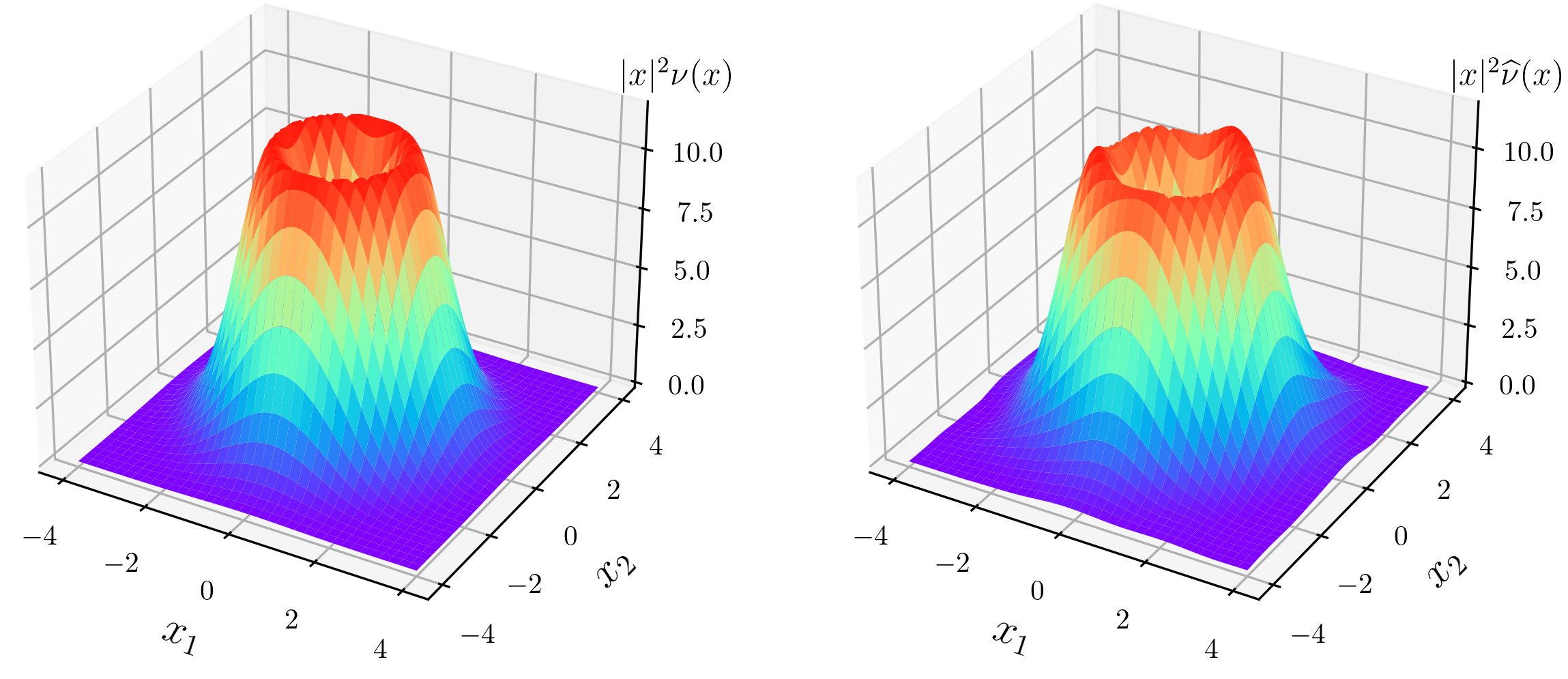
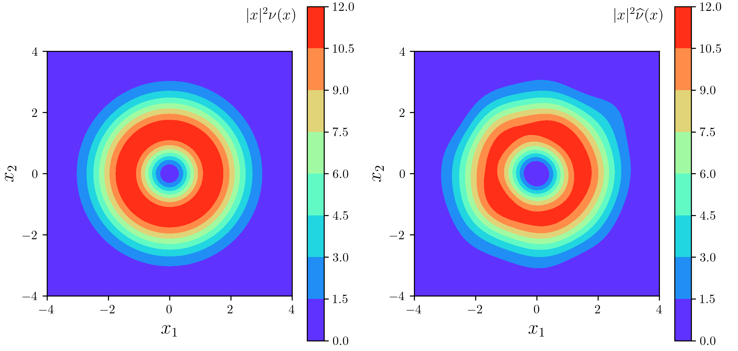
This theorem generalizes Trabs, 2015 to the multivariate case and additionally allows for high-frequency observations. Figs. 1 and 2 illustrate a simulation example of the estimation method.

In the mildly ill-posed case, one can easily attain the same rates without the logarithm when considering the pointwise loss.

We first discuss the low-frequency regime: For d=1d=1, our rates coincide with the proven minimax-optimal rates in the corresponding nonparametric deconvolution problems, see Fan, 1991. In the mildly ill-posed case with d=1d=1, the pointwise variant of our rate has been shown to be minimax-optimal under the assumption that xνx\nu is ss-Sobolev-regular, see Kappus, 2012. In the severely ill-posed case with d=1d=1 and α={1,2}\alpha=\{1,2\}, our rates coincide with the minimax-optimal rates of Neumann & Reiß, 2009, who consider the integrated risk in the estimation of Σδ0(dx)+|x|2(1+|x|2)1ν(dx)\Sigma\delta_{0}(\mathrm{d}x)+|x|^{2}(1+|x|^{2})^{-1}\nu(\mathrm{d}x) against test functions with Sobolev regularity ss. This measure has an atom in 00 and is therefore not smooth. Hence, the regularity in the rate comes purely from the test function. By considering UU bounded away from 00, we can profit from the regularity of the Lévy density outside the origin. We do not even suffer an additional loss for the dimension in the rate, only in the constant. Therefore, the above suggests its optimality.

One sees that the rates improve as the time grid narrows. If this refinement happens at an appropriate order compared to the growth of the sample, the ill-posedness vanishes completely in the mildly ill-posed case and the rate becomes polynomial in the severely ill-posed case. In the mildly ill-posed case with high-frequency observations, the rate corresponds to the minimax-optimal rate in a nonparametric regression.

It is straightforward to see from our proof, that when estimating ||2ν|\cdot|^{2}\nu , we can forgo the exclusion of the origin from UU while achieving the same rates in the mildly-ill-posed case. In the severely ill-posed case, the unknown volatility of the Brownian component of the Lévy process obstructs the observation of the small jumps. Hence, we can benefit from a pilot estimator for Σ\Sigma. As discussed earlier, even a with minimax-optimal estimator for Σ\Sigma, we would suffer a loss in the overall rate. However, in view of Eq. 6, it suffices to estimate the onedimensional parameter tr(Σ)\operatorname*{tr}(\Sigma) which is easier compared to the d×dd\times d-matrix Σ\Sigma. Following the spectral approach again, we propose the estimator

tr(Σ)^tr(Σ)^hWh(u)Δψn^(u)du.\widehat{\operatorname*{tr}(\Sigma)}\coloneqq\widehat{\operatorname*{tr}(\Sigma)}_{h}\coloneqq-\int W_{h}(u)\widehat{\Delta\psi_{n}}(u)\,\mathrm{d}u. (18)

where Wh=hdW(h)W_{h}=h^{d}W(h\cdot) for a bandwidth h>0h>0 (correspoding to the threshold h1h^{-1}) and a weight function W:dW\colon\mathbb{R}^{d}\to\mathbb{R} with

W(u)𝑑u=1andsuppW[1,1]d.\int W(u)\,\mathrm{d}u=1\qquad\text{and}\qquad\operatorname*{supp}W\subseteq[-1,1]^{d}. (19)

This estimator achieves a rate of (logT)(s+d)/α(\log T)^{-(s+d)/\alpha} and is incorporated into the estimator for ||2ν|\cdot|^{2}\nu via

||2ν^h1[Kh(Δψn^+tr(Σ)^h)]\widehat{|\cdot|^{2}\nu}_{h}\coloneqq-\mathcal{F}^{-1}\big[\mathcal{F}K_{h}\big(\widehat{\Delta\psi_{n}}+\widehat{\operatorname*{tr}(\Sigma)}_{h}\big)\big] (20)

leading to the following extension of 1.

test 0.

Let α,r,R,ζ,η>0,1<s,m>4\alpha,r,R,\zeta,\eta>0,1<s\in\mathbb{N},m>4 and let the kernel satisfy Eq. 9 with order psp\geqslant s as well as ||p+dKL1(d)|\cdot|^{p+d}K\in L^{1}(\mathbb{R}^{d}). Assume 1[W(x)/xks]L1<\|\mathcal{F}^{-1}[W(x)/x_{k}^{s}]\|_{L^{1}}<\infty for some kk. Choosing h=(log(T)/(4rδ))1/αh=(\log(T)/(4r\delta))^{-1/\alpha} we have uniformly in (Σ,γ,ν)s(α,m,d,r,R,ζ,η)(\Sigma,\gamma,\nu)\in\mathcal{E}^{s}(\alpha,m,\mathbb{R}^{d},r,R,\zeta,\eta)

supxd|(||2ν^h)(x)|x|2ν(x)|=𝒪((logT4rδ)s/α).\sup_{x^{\ast}\in\mathbb{R}^{d}}\big|\big(\widehat{|\cdot|^{2}\nu}_{h}\big)(x^{\ast})-|x^{\ast}|^{2}\nu(x^{\ast})\big|=\mathcal{O}_{\mathbb{P}}\Big(\Big(\frac{\log T}{4r\delta}\Big)^{-s/\alpha}\Big). (21)
Refer to caption
Figure 1: 3D plot of ||2ν|\cdot|^{2}\nu (left) and its estimate (right) for a twodimensional compound Poisson process with Gaussian jumps.
Refer to caption
Figure 2: Heatmap of ||2ν|\cdot|^{2}\nu (left) and its estimate (right) for a twodimensional compound Poisson process with Gaussian jumps.

2.2 Independent components

Compared to the onedimensional case, we need to take the dependence structure of the components of the process into account. In particular, our previous assumption about ν\nu having a Lebesgue-density on d\mathbb{R}^{d}, rules out Lévy processes where all components are independent, since the corresponding Lévy measure would only have mass on the coordinate cross. Similarly, Lévy processes consisting of multiple mutually independent blocks of components, where the components within the same block depend on each other, are not covered.For the sake of notational simplicity, we focus on the case of two equisized independent blocks: Let dd be even and L=(L(1),L(2))L=(L^{(1)},L^{(2)}), where L(1)L^{(1)} and L(2)L^{(2)} are two independent Lévy processes on d/2\mathbb{R}^{d/2} with characteristic triplets (Σ1,γ1,ν1)(\Sigma_{1},\gamma_{1},\nu_{1}) and (Σ2,γ2,ν2)(\Sigma_{2},\gamma_{2},\nu_{2}), respectively. Denoting by δ0\delta_{0} the Dirac-measure in 0d/20\in\mathbb{R}^{d/2}, it holds that

ν(dx)=ν1(dx(1))δ0(dx(2))+δ0(dx(1))ν2(dx(2))x=(x(1),x(2)),x(1),x(2)d/2.\nu(\mathrm{d}x)=\nu_{1}(\mathrm{d}x^{(1)})\otimes\delta_{0}(\mathrm{d}x^{(2)})+\delta_{0}(\mathrm{d}x^{(1)})\otimes\nu_{2}(\mathrm{d}x^{(2)})\qquad x=(x^{(1)},x^{(2)}),\>x^{(1)},x^{(2)}\in\mathbb{R}^{d/2}.\addcontentsline{lla}{section}{\numberline q:nu_{m}isspec} (22)

We summarize the class of such Lévy processes as

𝒞~(m,R)\displaystyle\widetilde{\mathcal{C}}(m,R) {(Σ,γ,ν)|Σ=(Σ100Σ2),tr(Σ)R,Σ1,Σ2d/2×d/2 positive-semidefinite,γd,\displaystyle\coloneqq\Big\{(\Sigma,\gamma,\nu)\,\Big|\,\Sigma=\Big(\!\!\!\begin{array}[]{cc}\Sigma_{1}&0\\ 0&\Sigma_{2}\end{array}\!\!\!\Big),\operatorname*{tr}(\Sigma)\leqslant R,\Sigma_{1},\Sigma_{2}\in\mathbb{R}^{d/2\times d/2}\text{ positive-semidefinite},\gamma\in\mathbb{R}^{d},
|x|mν(𝑑x)R,ν has the form Eq. 22 and v1,ν2 have Lebesgue-densities}\displaystyle\qquad\qquad\qquad\qquad\int|x|^{m}\,\nu(\mathrm{d}x)\leqslant R,\nu\text{ has the form \lx@cref{creftype\lx@tilde refnum}{eq:nu_misspec} and $v_{1},\nu_{2}$ have Lebesgue-densities$\Big\}$} (25)

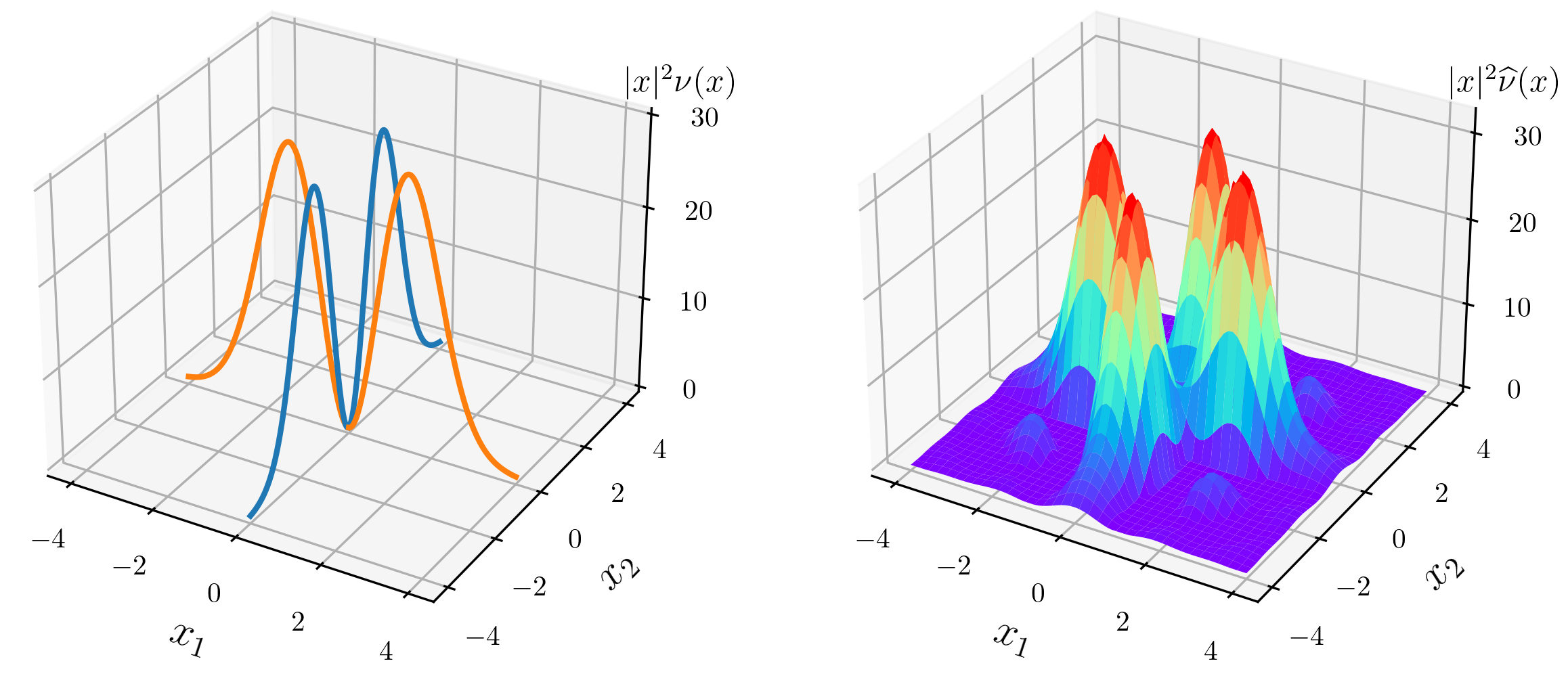
for m,R>0m,R>0. A simple example of such a Lévy measure and its estimate are illustrated in Fig. 3.

As before, we distinguish between the mildly ill-posed case with α>0\alpha>0

𝒟~(α,m,R){(0,γ,ν)𝒞~(m,R)|(1+||)α/φ1R,|xk|νkR,k=1,2}\widetilde{\mathcal{D}}(\alpha,m,R)\coloneqq\big\{(0,\gamma,\nu)\in\widetilde{\mathcal{C}}(m,R)\,\big|\,\|(1+|\cdot|_{\infty})^{-\alpha}/\varphi_{1}\|_{\infty}\leqslant R,\,\||x_{k}|\nu_{k}\|_{\infty}\leqslant R,k=1,2\big\} (26)

and the severely ill-posed case with α,r,η>0\alpha,r,\eta>0

~(α,m,r,R,η){(Σ,γ,ν)𝒞~(m,R)|exp(r||α)/φ1R,|xk|3ηνk(xk)R|xk|1,k=1,2}\widetilde{\mathcal{E}}(\alpha,m,r,R,\eta)\coloneqq\big\{(\Sigma,\gamma,\nu)\in\widetilde{\mathcal{C}}(m,R)\,\big|\,\|\exp(-r|\cdot|_{\infty}^{\alpha})/\varphi_{1}\|_{\infty}\leqslant R,|x_{k}|^{3-\eta}\nu_{k}(x_{k})\leqslant R\;\forall|x_{k}|\leqslant 1,k=1,2\big\} (27)

based on the decay behavior of the characteristic function and the presence of a Gaussian component.

If this dependence structure were known, we could seperate the blocks in the observations, apply our method to each block and obtain an estimator for the overall Lévy measure. Since this is not the case, we are left with applying our initial method. In spite of the unknown dependence structure, we will be able to quantify the estimation error. Due to the structure of the Lévy measure, we cannot hope for a pointwise quantitative bound. Instead, we consider the error in a functional sense. To this end, we introduce the following class of test functions for ϱ>0\varrho>0 and UdU\subseteq\mathbb{R}^{d}

Fϱ(U,R){f:dfCϱ(d),fCϱ(d),fL1(d)R,suppfU}.F_{\varrho}(U,R)\coloneqq\{f\colon\mathbb{R}^{d}\to\mathbb{R}\mid f\in C^{\varrho}(\mathbb{R}^{d}),\|f\|_{C^{\varrho}(\mathbb{R}^{d})},\|f\|_{L^{1}(\mathbb{R}^{d})}\leqslant R,\,\operatorname*{supp}f\subseteq U\}. (28)
Refer to caption
Figure 3: 3D plot of ||2ν|\cdot|^{2}\nu (left) and its estimate (right) for a Lévy-process where both components are independent compound Poisson processes with Gaussian jumps.
test 3.

Let α,r,R>0,ϱ>1,m>4\alpha,r,R>0,\varrho>1,m>4, let the kernel have product structure and satisfy Eq. 9 with order pϱp\geqslant\varrho. Then, we have for 0<δR,n0<\delta\leqslant R,n\to\infty:

  1. (M)

    If UdU\subseteq\mathbb{R}^{d} is bounded and h=(log(T)/T)1/(2ϱ+2δα+3d/2)h=(\log(T)/T)^{1/(2\varrho+2\delta\alpha+3d/2)}, then uniformly in (Σ,γ,ν)𝒟~(α,m,R)(\Sigma,\gamma,\nu)\in\widetilde{\mathcal{D}}(\alpha,m,R)

    supfFϱ(U,R)|Uf(x)|x|2(ν(𝑑x)ν^h(𝑑x))|=𝒪((logTT)ϱ/(2ϱ+2δα+3d/2)).\sup_{f\in F_{\varrho}(U,R)}\Big|\int_{U}f(x)|x|^{2}\big(\nu(\mathrm{d}x)-\widehat{\nu}_{h}(\mathrm{d}x)\big)\Big|=\mathcal{O}_{\mathbb{P}}\Big(\Big(\frac{\log T}{T}\Big)^{\varrho/(2\varrho+2\delta\alpha+3d/2)}\Big). (29)
  2. (S)

    If UdU\subseteq\mathbb{R}^{d} is bounded away from 00, ||p+dKL1(d)|\cdot|^{p+d}K\in L^{1}(\mathbb{R}^{d}), η>0\eta>0 and h=(log(T)/(4rδ))1/αh=(\log(T)/(4r\delta))^{-1/\alpha}, then uniformly in (Σ,γ,ν)~(α,m,r,R,η)(\Sigma,\gamma,\nu)\in\widetilde{\mathcal{E}}(\alpha,m,r,R,\eta)

    supfFϱ(U,R)|Uf(x)|x|2(ν(dx)ν^h(dx))|=𝒪((logT4rδ)ϱ/α).\sup_{f\in F_{\varrho}(U,R)}\Big|\int_{U}f(x)|x|^{2}\big(\nu(\mathrm{d}x)-\widehat{\nu}_{h}(\mathrm{d}x)\big)\Big|=\mathcal{O}_{\mathbb{P}}\Big(\Big(\frac{\log T}{4r\delta}\Big)^{-\varrho/\alpha}\Big). (30)

Note that the regularity parameter ϱ\varrho in the rates comes from the smoothness of the test functions as compared to the smoothness ss of the Lévy measure in 1. In the severely ill-posed case, the result is analogous to the well-specified. In the mildly ill-posed case, we pay for the dependence structure with an d/2d/2 in the rate. Morally, one can interpret this as the model dimension being 3d/23d/2 instead of dd.

Remark 4.

The product kernel is compatible with any dependence structure of blocks, regardless of their size. For instance, if all components of the process are independent, one gets still gets the analogous result in severely ill-posed case. In the mildly ill-posed case, the dimension appearing in the rate is 2d12d-1 instead of 3d/23d/2. Comparing the dependence structures, one finds that the two independent blocks are an in-between case of no independent blocks and fully independent components.

2.3 A uniform risk-bound for the characteristic function and linearization

A key ingredient in the proofs of our preceeding results is the following moment-uniform risk bound for the multivariate characteristic function and its partial derivatives. It generalizes the existing results in the univariate case (see Kappus & Reiß, 2010) and the multivariate non-uniform case (see Belomestny & Trabs, 2018).

test 0.

Let X1,X2,X_{1},X_{2},\dots be d\mathbb{R}^{d}-valued i.i.d. random variables with characteristic function φ\varphi and empirical characteristic function φ^n\widehat{\varphi}_{n} such that 𝔼[|X1|2β|X1|τ]ρ|β|11\mathbb{E}[|X_{1}|^{2\beta}|X_{1}|^{\tau}]\lesssim\rho^{|\beta|_{1}\land 1} and 𝔼[|X1|2β]ρ|β|11\mathbb{E}[|X_{1}|^{2\beta}]\lesssim\rho^{|\beta|_{1}\wedge 1} for some multi-index β0d\beta\in\mathbb{N}_{0}^{d} and τ,ρ>0\tau,\rho>0. For the inverse softplus-type weight function w(u)=log(e+|u|)(1+χ)/2w(u)=\log(\mathrm{e}+|u|)^{-(1+\chi)/2} with χ>0\chi>0, we have

𝔼[w(u)(φ^nφ)(β)(u)]ρ(|β|11)/2n1/2.\mathbb{E}\big[\big\|w(u)(\widehat{\varphi}_{n}-\varphi)^{(\beta)}(u)\big\|_{\infty}\big]\lesssim\rho^{(|\beta|_{1}\land 1)/2}n^{-1/2}. (31)

As a direct consequence of 5, the indicator in the definition Eq. 7 equals one on the support of Kh\mathcal{F}K_{h}, with probability converging to one for the bandwidths we consider.

To prove our rates for ν^h\widehat{\nu}_{h}, Eq. 6 lets us decompose the error

ν^h\displaystyle\widehat{\nu}_{h} (x)ν(x)\displaystyle(x^{\ast})-\nu(x^{\ast})
=|x|2((Kh(||2ν)||2ν)(x)1[Kh(Δψn^Δψ)](x)+tr(Σ)Kh(x))\displaystyle\negthickspace\negthickspace\negthickspace\negthickspace=|x^{\ast}|^{-2}\big(\big(K_{h}\ast(|\cdot|^{2}\nu)-|\cdot|^{2}\nu\big)(x^{\ast})-\mathcal{F}^{-1}\big[\mathcal{F}K_{h}\big(\widehat{\Delta\psi_{n}}-\Delta\psi\big)\big](x^{\ast})+\operatorname*{tr}(\Sigma)K_{h}(x^{\ast})\big)
=|x|2((Kh(||2ν)||2ν)(x)Bν(x)1δ1[KhΔ((φ^δ,nφδ)/φδ)](x)Lδ,nν(x)+Rδ,n+tr(Σ)Kh(x))\displaystyle\negthickspace\negthickspace\negthickspace\negthickspace=|x^{\ast}|^{-2}\big(\underbrace{\big(K_{h}\ast(|\cdot|^{2}\nu)-|\cdot|^{2}\nu\big)(x^{\ast})}_{\eqqcolon B^{\nu}(x^{\ast})}-\underbrace{\frac{1}{\delta}\mathcal{F}^{-1}\big[\mathcal{F}K_{h}\Delta\big((\widehat{\varphi}_{\delta,n}-\varphi_{\delta})/\varphi_{\delta}\big)\big](x^{\ast})}_{\eqqcolon L_{\delta,n}^{\nu}(x^{\ast})}+R_{\delta,n}+\operatorname*{tr}(\Sigma)K_{h}(x^{\ast})\big) (32)

into a bias term BνB^{\nu}, the linearized stochastic error Lδ,nνL_{\delta,n}^{\nu}, the error tr(Σ)Kh\operatorname*{tr}(\Sigma)K_{h} due to the volatility and a remainder term Rδ,nR_{\delta,n}. 5 applied to the increments of the Lévy process leads to the following linearization.

test 0.

Let |x|4+τν(𝑑x)R\int|x|^{4+\tau}\,\nu(\mathrm{d}x)\leqslant R for some τ>0\tau>0. If n1/2(logh1)(1+χ)/2φδ1L(Ih)0n^{-1/2}(\log h^{-1})^{(1+\chi)/2}\|\varphi_{\delta}^{-1}\|_{L^{\infty}(I_{h})}\to 0 as nn\to\infty for h(0,1),χ>0h\in(0,1),\chi>0, it holds

sup|u|h1|Δψn^(u)\displaystyle\sup_{|u|_{\infty}\leqslant h^{-1}}\big|\widehat{\Delta\psi_{n}}(u) Δψ(u)δ1Δ((φ^δ,nφδ)/φδ)(u)|=𝒪(an),where\displaystyle-\Delta\psi(u)-\delta^{-1}\Delta\big((\widehat{\varphi}_{\delta,n}-\varphi_{\delta})/\varphi_{\delta}\big)(u)\big|=\mathcal{O}_{\mathbb{P}}(a_{n}),\qquad\text{where}
an\displaystyle a_{n} n1(logh1)1+χφδ1L(Ih)2δ1/2(δ|ψ|L(Ih)+δ3/2|ψ|L(Ih)2+1).\displaystyle\coloneqq n^{-1}(\log h^{-1})^{1+\chi}\|\varphi_{\delta}^{-1}\|_{L^{\infty}(I_{h})}^{2}\delta^{-1/2}\big(\delta\big\||\nabla\psi|\big\|_{L^{\infty}(I_{h})}+\delta^{3/2}\big\||\nabla\psi|\big\|_{L^{\infty}(I_{h})}^{2}+1\big). (33)

As a direct consequence, the remainder term is of the order

|Rδ,n|=𝒪(hdan).|R_{\delta,n}|=\mathcal{O}_{\mathbb{P}}\big(h^{-d}a_{n}\big).\addcontentsline{lla}{section}{\numberline q:remainderorder} (34)

After treating the four terms in Eq. 32, the asserted rates follow from our bandwidth choices.

3 Simulation examples

We demonstrate the estimation of the Lévy density for d=2d=2 with three examples: a compound Poisson process, a variance gamma process and two independent compound Poisson processes.

A challenge is to find examples of multivariate Lévy processes for which paths can be simulated and the true Lévy measure is accessible (at least numerically). To allow for plotable results, we consider the case d=2d=2 and compensate for the possible singularity of the Lévy density at the origin, i.e. we plot ||2ν|\cdot|^{2}\nu and its estimate. Throughout, we use the flat-top-kernel KK, see McMurry & Politis, 2004, as defined by its Fourier transform

K(u){1,|u|c,exp(bexp(b/(|u|c)2(|u|1)2)c<|u|<1,0,|u|1,\mathcal{F}K(u)\coloneqq\begin{cases}1,&|u|\leqslant c,\\ \exp\Big(-\frac{b\exp(-b/(|u|-c)^{2}}{(|u|-1)^{2}}\Big)&c<|u|<1,\\ 0,&|u|\geqslant 1,\end{cases} (35)

whose decay behaviour is controlled by b>0b>0 and 0<c<10<c<1. In our simulations, b=1,c=1/50b=1,c=1/50 deliver stable results. While a product kernel is convenient for theoretical reasons in Section 2.2, it did not seem necessary in practice. Throughout, we simulate increments of the processes with a time difference of δ=0.001\delta=0.001 and fix the bandwidth at h=4T1/2h=4T^{-1/2}. To conquer this ill-posed problem, we use large samples of n=500,000n=500,000 increments. From the definition Eq. 8 of the estimator, it is not guaranteed that ν^0\widehat{\nu}\geqslant 0 and for numerical reasons even ν^\widehat{\nu}\in\mathbb{C}\setminus\mathbb{R} is possible in practice. Therefore, we consider the estimator Re(ν^)0\operatorname*{Re}(\widehat{\nu})\lor 0 in our simulations.

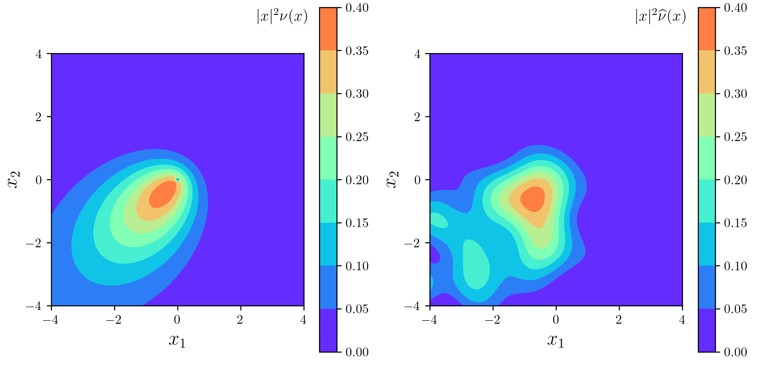
The most straightforward example under consideration is the compound Poisson process with intensity λ=100\lambda=100 and twodimensional standard-Gaussian jumps. In this case, the Lévy density is just the standard normal density, rescaled with the intensity λ\lambda. Fig. 1 illustrates that the method captures the overall shape of the density. The heatmap in Fig. 2 provides a more detailed view especially around the origin. We observe that the decay for |x||x|\to\infty and |x|0|x|\searrow 0 is well-estimated, with slight problems only arising on an annulus around the origin.

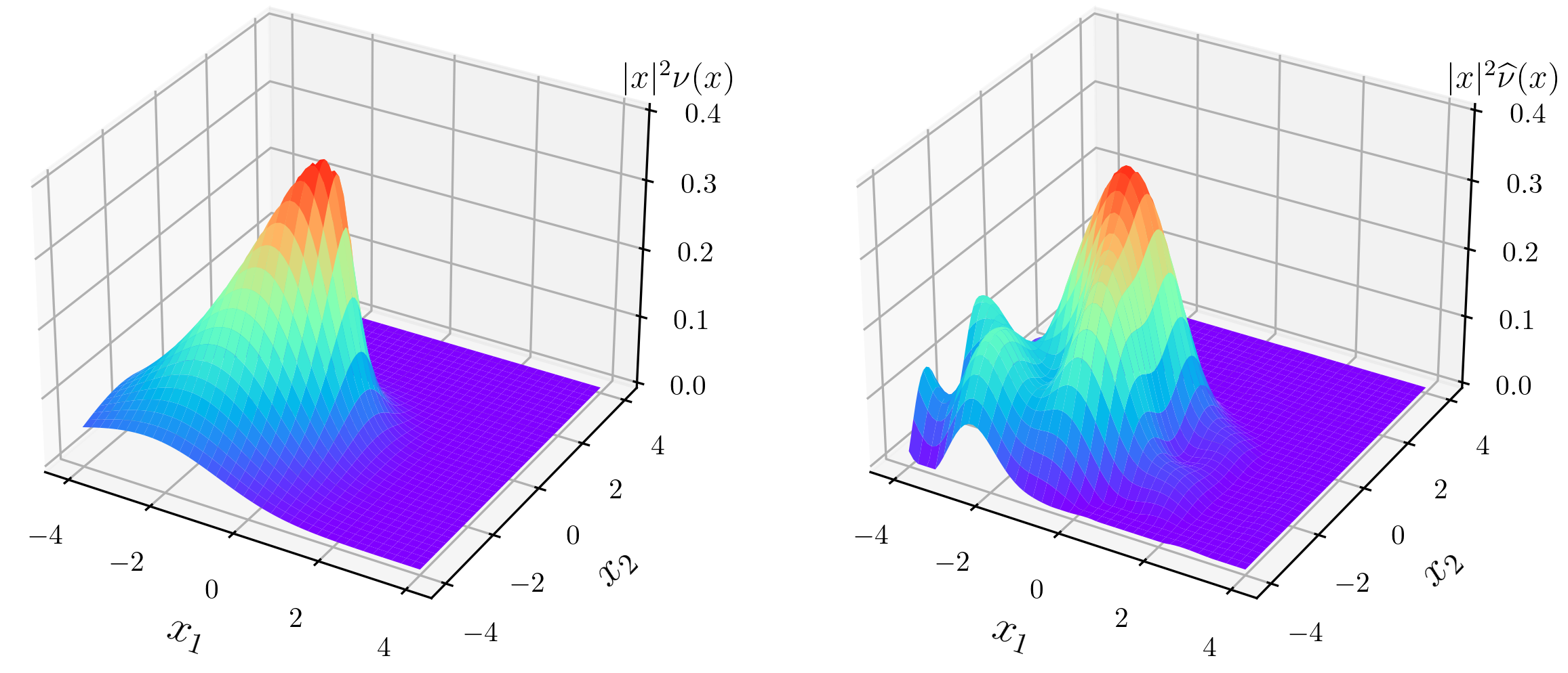
A practical way to construct easy-to-simulate multivariate Lévy processes is to subordinate multivariate Brownian motion. In particular, we use a gamma process with variance κ=1\kappa=1 to subordinate a twodimensional standard Brownian motion. To access the Lévy measure of the resulting variance gamma process, we approximate the theoretical expression from Cont & Tankov, 2004 numerically. The results are again illustrated in a 3D plot (Fig. 4) and as a heatmap ((Fig. 5)). In this example, the estimator suffers from oscillations around the true density which are to be expected from spectral-based methods.

To demonstrate the method under the depencence structure discussed in (Section 2.2), we consider a Lévy process comprised of two independent compound Poisson processes, each with intensity λ=100\lambda=100 and onedimensional standard-Gaussian jumps. In contrast to the twodimensional compound Poisson process at the considered at the beginnung of this section, the jumps in both components are driven by independent Poisson processes. The corresponding Lévy measure takes the form Eq. 22, where ν1\nu_{1} and ν2\nu_{2} are onedimensional standard-Gaussian densities, rescaled with λ\lambda, as illustrated on the left hand side of Fig. 3. It is important to emphasize, that the blue and the orange line represent the Lebesgue-densities of both components on \mathbb{R}, not 2\mathbb{R}^{2}. The right hand side of the aforementioned figure reveals a strong performance of the estimator on the coordinate cross. Around the axes, we observe a smearing effect due to the singularity of the true Lévy measure on the coordinate cross before the estimate drops off as we move away.
Refer to caption
Figure 4: 3D plot of ||2ν|\cdot|^{2}\nu (left) and its estimate (right) for a twodimensional variance gamma process.
Refer to caption
Figure 5: Heatmap of ||2ν|\cdot|^{2}\nu (left) and its estimate (right) for a twodimensional variance gamma process.

4 Proofs

Throughout, set Ih[h1,h1]dI_{h}\coloneqq[-h^{-1},h^{-1}]^{d} for h>0h>0. Note that Σ,ν,Δψ\Sigma,\nu,\Delta\psi and Δψn^\widehat{\Delta\psi_{n}} do not change if we consider increments based on the Lévy process (Lttγ0)t0(L_{t}-t\gamma_{0})_{t\geqslant 0} for some γ0d\gamma_{0}\in\mathbb{R}^{d}. Hence, no generality is lost if we choose γ0\gamma_{0} such that in the mildly ill-posed case

ψ=i[xν]andΔψ=[|x|2ν]\nabla\psi=\mathrm{i}\mathcal{F}[x\nu]\qquad\qquad\text{and}\qquad\qquad\Delta\psi=-\mathcal{F}[|x|^{2}\nu]\addcontentsline{lla}{section}{\numberline q:psigradwlog} (36)

and in the severely ill-posed case γ=0\gamma=0, see Nickl et al., 2016 for a similar argument in the onedimensional case.

Further, due to the infinite divisibility of ν\nu, the decay behavior of φ1\varphi_{1} governs that of φδ\varphi_{\delta}. In particular, we have for 0<δR0<\delta\leqslant R

(1+||)δα/φδ(1R)Randexp(rδ||α)/φδ(1R)R\|(1+|\cdot|_{\infty})^{-\delta\alpha}/\varphi_{\delta}\|_{\infty}\leqslant(1\vee R)^{R}\qquad\text{and}\qquad\|\exp(-r\delta|\cdot|_{\infty}^{\alpha})/\varphi_{\delta}\|_{\infty}\leqslant(1\vee R)^{R} (37)

in the mildly and the severely ill-posed case, respectively.

4.1 Proof of 1

We extend the proof strategy by Trabs, 2015 to accomodate for the multivariate setting. To allow for the application to high-frequency observations, we carefully keep track of δ\delta throughout. Subsequently, we will analyze the four terms in Eq. 32.

4.1.1 Controlling the linearized stochastic error

To control

Lδ,nν1[Khδ1Δ((φ^δ,nφδ)/φδ)]L_{\delta,n}^{\nu}\coloneqq\mathcal{F}^{-1}\big[\mathcal{F}K_{h}\delta^{-1}\Delta\big((\widehat{\varphi}_{\delta,n}-\varphi_{\delta})/\varphi_{\delta}\big)\big] (38)

we need to get a grip on the partial derivatives of φ^δ,nφδ\widehat{\varphi}_{\delta,n}-\varphi_{\delta} in the Laplacian of (φ^δ,nφδ)/φδ(\widehat{\varphi}_{\delta,n}-\varphi_{\delta})/\varphi_{\delta}. In particular, we will show that

supud𝔼[|lukl(φ^δ,nφδ)(u)|]supud𝔼[|lukl(φ^δ,nφδ)(u)|2]1/2!n1/2δ(l1)/2,l=0,1,2.\sup_{u\in\mathbb{R}^{d}}\mathbb{E}\Big[\Big|\frac{\partial^{l}}{\partial u_{k}^{l}}(\widehat{\varphi}_{\delta,n}-\varphi_{\delta})(u)\Big|\Big]\leqslant\sup_{u\in\mathbb{R}^{d}}\mathbb{E}\Big[\Big|\frac{\partial^{l}}{\partial u_{k}^{l}}(\widehat{\varphi}_{\delta,n}-\varphi_{\delta})(u)\Big|^{2}\Big]^{1/2}\stackrel{{\scriptstyle!}}{{\lesssim}}n^{-1/2}\delta^{(l\land 1)/2},\qquad l=0,1,2.\addcontentsline{lla}{section}{\numberline q:moments} (39)

Since

𝔼[|lukl(φ^δ,nφδ)(u)|]n1𝔼[Y1,m2l]=n1|2luk2lφδ(0)|ud,\mathbb{E}\Big[\Big|\frac{\partial^{l}}{\partial u_{k}^{l}}(\widehat{\varphi}_{\delta,n}-\varphi_{\delta})(u)\Big|\Big]\leqslant n^{-1}\mathbb{E}[Y_{1,m}^{2l}]=n^{-1}\Big|\frac{\partial^{2l}}{\partial u_{k}^{2l}}\varphi_{\delta}(0)\Big|\qquad\forall u\in\mathbb{R}^{d}, (40)

where Y1,kY_{1,k} denotes the kk-th entry of Y1Y_{1}, the case l=0l=0 is obvious and for l=1,2l=1,2 it remains to show

|2luk2lφδ(0)|δ.\Big|\frac{\partial^{2l}}{\partial u_{k}^{2l}}\varphi_{\delta}(0)\Big|\lesssim\delta. (41)

In the mildly ill-posed case

|ukψ(0)||xk|ν(𝑑x)|x|ν(𝑑x)1\Big|\frac{\partial}{\partial u_{k}}\psi(0)\Big|\lesssim\int|x_{k}|\,\nu(\mathrm{d}x)\leqslant\int|x|\,\nu(\mathrm{d}x)\lesssim 1 (42)

and in the severely ill-posed case

ukψ(0)=0.\frac{\partial}{\partial u_{k}}\psi(0)=0. (43)

The product rule for higher order derivatives yields

|2φδuk2(0)|\displaystyle\Big|\frac{\partial^{2}\varphi_{\delta}}{\partial u_{k}^{2}}(0)\Big| =|δφδ(u)(δ(ukψ(u))2+2uk2ψ(u))|u=0δ(1+|x|2ν(𝑑x))δand\displaystyle=\Big|\delta\varphi_{\delta}(u)\Big(\delta\Big(\frac{\partial}{\partial u_{k}}\psi(u)\Big)^{2}+\frac{\partial^{2}}{\partial u_{k}^{2}}\psi(u)\Big)\Big|_{u=0}\lesssim\delta\Big(1+\int|x|^{2}\,\nu(\mathrm{d}x)\Big)\lesssim\delta\qquad\text{and} (44)
|4φδuk4(0)|\displaystyle\Big|\frac{\partial^{4}\varphi_{\delta}}{\partial u_{k}^{4}}(0)\Big| =|2uk2(2φδuk2(u))(0)|δj=02(2j)|𝔼[Y1,k2j]|(|jukj(ψuk(u))2|u=0+|j+2ψukj+2(0)|)δ,\displaystyle=\Big|\frac{\partial^{2}}{\partial u_{k}^{2}}\Big(\frac{\partial^{2}\varphi_{\delta}}{\partial u_{k}^{2}}(u)\Big)(0)\Big|\lesssim\delta\sum_{j=0}^{2}\binom{2}{j}|\mathbb{E}[Y_{1,k}^{2-j}]|\Big(\Big|\frac{\partial^{j}}{\partial u_{k}^{j}}\Big(\frac{\partial\psi}{\partial u_{k}}(u)\Big)^{2}\Big|_{u=0}+\Big|\frac{\partial^{j+2}\psi}{\partial u_{k}^{j+2}}(0)\Big|\Big)\lesssim\delta, (45)

where all emerging partial derivatives can again be absolutely and uniformly bounded using our assumptions on ν\nu.

To simplify the notation, set mδ,hKh/φδm_{\delta,h}\coloneqq\mathcal{F}K_{h}/\varphi_{\delta} and recall xyk=1dxkykx\cdot y\coloneqq\sum_{k=1}^{d}x_{k}y_{k} for x,ydx,y\in\mathbb{C}^{d}.

For the severely ill-posed case, we have |Δψ(u)|1|\Delta\psi(u)|\lesssim 1 and that |eiu,x1||x||u||\mathrm{e}^{\mathrm{i}\langle u,x\rangle}-1|\leqslant|x||u| implies |ψ(u)||u||\nabla\psi(u)|\lesssim|u|. Together with Eq. 39, we obtain

𝔼[supxd|Lδ,nν(x)|]\displaystyle\mathbb{E}\Big[\sup_{x^{\ast}\in\mathbb{R}^{d}}|L_{\delta,n}^{\nu}(x^{\ast})|\Big] δ1𝔼[1[mδ,hΔ(φ^δ,nφδ)]]+2𝔼[1[mδ,h(φ^δ,nφδ)ψ]]\displaystyle\leqslant\delta^{-1}\mathbb{E}\big[\big\|\mathcal{F}^{-1}[m_{\delta,h}\Delta(\widehat{\varphi}_{\delta,n}-\varphi_{\delta})]\big\|_{\infty}\big]+2\mathbb{E}\big[\big\|\mathcal{F}^{-1}[m_{\delta,h}\nabla(\widehat{\varphi}_{\delta,n}-\varphi_{\delta})\cdot\nabla\psi]\big\|_{\infty}\big]
+𝔼[1[mδ,h(φ^δ,nφδ)(δ(ψ)2Δψ)]]\displaystyle\qquad\qquad\qquad+\mathbb{E}\big[\big\|\mathcal{F}^{-1}[m_{\delta,h}(\widehat{\varphi}_{\delta,n}-\varphi_{\delta})(\delta(\nabla\psi)^{2}-\Delta\psi)]\big\|_{\infty}\big]
(2π)dIh(δ1𝔼[|Δ(φ^δ,nφδ)(u)|]+𝔼[|(φ^δ,nφδ)(u)ψ(u)|]CLOSE\displaystyle\lesssim(2\pi)^{-d}\int_{I_{h}}\Big(\delta^{-1}\mathbb{E}\big[\big|\Delta(\widehat{\varphi}_{\delta,n}-\varphi_{\delta})(u)\big|\big]+\mathbb{E}\big[\big|\nabla(\widehat{\varphi}_{\delta,n}-\varphi_{\delta})(u)\cdot\nabla\psi(u)\big|\big]
OPEN+𝔼[|(φ^δ,nφδ)(u)|](|Δψ(u)|+δ|ψ(u)|2))exp(rδ|u|α)du\displaystyle\qquad\qquad\qquad+\mathbb{E}\big[\big|(\widehat{\varphi}_{\delta,n}-\varphi_{\delta})(u)\big|\big]\big(|\Delta\psi(u)|+\delta|\nabla\psi(u)|^{2}\big)\Big)\exp(r\delta|u|_{\infty}^{\alpha})\,\mathrm{d}u
πdT1/2Ih(1+δ|u|+δ1/2+δ3/2|u|2)exp(rδ|u|α)du\displaystyle\lesssim\pi^{-d}T^{-1/2}\int_{I_{h}}\big(1+\delta|u|+\delta^{1/2}+\delta^{3/2}|u|^{2}\big)\exp(r\delta|u|_{\infty}^{\alpha})\,\mathrm{d}u
T1/2(hd+δhd1+δ3/2hd2)exp(rδhα),\displaystyle\lesssim T^{-1/2}\big(h^{-d}+\delta h^{-d-1}+\delta^{3/2}h^{-d-2}\big)\exp(r\delta h^{-\alpha}), (46)

which will be dominated by the bias.

In the mildly ill-posed case, the stochastic error needs to be decomposed further into the main stochastic error

Mδ,nν\displaystyle M_{\delta,n}^{\nu} 1Tk=1n1[mδ,h(|Yk|2eiu,Yk𝔼[|Yk|2eiu,Yk])]and\displaystyle\coloneqq-\frac{1}{T}\sum_{k=1}^{n}\mathcal{F}^{-1}\Big[m_{\delta,h}\big(|Y_{k}|^{2}\mathrm{e}^{\mathrm{i}\langle u,Y_{k}\rangle}-\mathbb{E}\big[|Y_{k}|^{2}\mathrm{e}^{\mathrm{i}\langle u,Y_{k}\rangle}\big]\big)\Big]\qquad\text{and}
Mδ,nνLδ,nν\displaystyle M_{\delta,n}^{\nu}-L_{\delta,n}^{\nu} =21[mδ,h(φ^δ,nφδ)ψ]+1[mδ,h(φ^δ,nφδ)(Δψδ(ψ)2)].\displaystyle\hskip 1.99997pt=2\mathcal{F}^{-1}\big[m_{\delta,h}\nabla(\widehat{\varphi}_{\delta,n}-\varphi_{\delta})\cdot\nabla\psi\big]+\mathcal{F}^{-1}\big[m_{\delta,h}(\widehat{\varphi}_{\delta,n}-\varphi_{\delta})\big(\Delta\psi-\delta(\nabla\psi)^{2}\big)\big]. (47)

To control the difference Eq. 47, note that |x|νR\||x|\nu\|_{\infty}\leqslant R and |x|mνL1R\||x|^{m}\nu\|_{L^{1}}\leqslant R imply |x|νL1\||x|\nu\|_{L^{1}}, |x|νL2\||x|\nu\|_{L^{2}}, |x|2νL21\||x|^{2}\nu\|_{L^{2}}\lesssim 1. Further, the support of K\mathcal{F}K and the decay behavior of φδ\varphi_{\delta} ensure

mδ,hL22|K(hu)|2(1+|u|)2δα𝑑u(1+h1)2δαhdh2δαd.\|m_{\delta,h}\|_{L^{2}}^{2}\lesssim\int|\mathcal{F}K(hu)|^{2}(1+|u|)^{2\delta\alpha}\,\mathrm{d}u\lesssim(1+h^{-1})^{2\delta\alpha}h^{-d}\lesssim h^{-2\delta\alpha-d}.\addcontentsline{lla}{section}{\numberline q:m_{o}rder} (48)

Hence, Eq. 39 and the Cauchy-Schwarz inequality together with Eq. 36 and the Plancherel theorem and Eq. 36 lead to

𝔼[supxU|Mδ,nν(x)Lδ,nν(x)|]\displaystyle\mathbb{E}\Big[\sup_{x^{\ast}\in U}\big|M_{\delta,n}^{\nu}(x^{\ast})-L_{\delta,n}^{\nu}(x^{\ast})\big|\Big] (2π)d(2𝔼[mδ,h(φ^δ,nφδ)ψL1]\displaystyle\leqslant(2\pi)^{-d}\big(2\mathbb{E}\big[\big\|m_{\delta,h}\nabla(\widehat{\varphi}_{\delta,n}-\varphi_{\delta})\cdot\nabla\psi\big\|_{L^{1}}\big]
OPEN+𝔼[mδ,h(φ^δ,nφδ)(Δψδ(ψ)2)L1])\displaystyle\qquad\qquad\qquad+\mathbb{E}\big[\big\|m_{\delta,h}(\widehat{\varphi}_{\delta,n}-\varphi_{\delta})\big(\Delta\psi-\delta(\nabla\psi)^{2}\big)\big\|_{L^{1}}\big]\big)
n1/2mδ,hL2(δ1/2|x|νL2+|x|2νL2+δd2|x|νL2|x|νL1)\displaystyle\lesssim n^{-1/2}\|m_{\delta,h}\|_{L^{2}}\big(\delta^{1/2}\||x|\nu\|_{L^{2}}+\||x|^{2}\nu\|_{L^{2}}+\delta d^{2}\||x|\nu\|_{L^{2}}\||x|\nu\|_{L^{1}}\big)
n1/2hδαd/2.\displaystyle\lesssim n^{-1/2}h^{-\delta\alpha-d/2}. (49)

Being the sum of centered i.i.d. random variables, the main stochastic error for fixed xx is controlled by Bernstein’s inequality as summarized in the following lemma.

test 0.

Let α,R,ζ>0,m>4\alpha,R,\zeta>0,m>4 and xdx\in\mathbb{R}^{d} and let the kernel satisfy Eq. 9 for p1p\geqslant 1. If (Σ,γ,ν)𝒟s(α,m,U,R,ζ)(\Sigma,\gamma,\nu)\in\mathcal{D}^{s}(\alpha,m,U,R,\zeta), then there exists some constant c>0c>0 depending only on R,αR,\alpha and dd such that for any κ0>0\kappa_{0}>0 and any n,0<δR,h(0,1)n\in\mathbb{N},0<\delta\leqslant R,h\in(0,1)

(|Mδ,nν(x)|κ0T1/2hδαd/2)2exp(cκ02(1+|x|3)(1+κ0(hdT)1/2)).\mathbb{P}\big(|M_{\delta,n}^{\nu}(x)|\geqslant\kappa_{0}T^{-1/2}h^{-\delta\alpha-d/2}\big)\leqslant 2\exp\Big(-\frac{c\kappa_{0}^{2}}{(1+|x|^{3})\big(1+\kappa_{0}(h^{d}T)^{-1/2}\big)}\Big). (50)

To establish a uniform bound for xUx^{\ast}\in U, a union bound extends this lemma to a discretization of the bounded set UU and Lipschitz continuity of xMδ,nν(x)x\mapsto M_{\delta,n}^{\nu}(x) allows us to control the discretization error. In particular, a standard covering argument yields a discretization x1,,xNndx_{1},\dots,x_{N_{n}}\in\mathbb{R}^{d} of UU such that supxUminl=1,,Nn|xxl|T2\sup_{x^{\ast}\in U}\min_{l=1,\dots,N_{n}}|x^{\ast}-x_{l}|\leqslant T^{-2}, NnT2dN_{n}\lesssim T^{2d} and maxl=1,,Nn|xl|C\max_{l=1,\dots,N_{n}}|x_{l}|\leqslant C with some C>0C>0 indepedent of nn. Since

Mδ,nν\displaystyle M_{\delta,n}^{\nu} =Khgwithgδ11[𝟙Ihφδ1Δ(φ^δ,nφδ)],\displaystyle=K_{h}\ast g\qquad\text{with}\qquad g\coloneqq\delta^{-1}\mathcal{F}^{-1}\big[\mathbbm{1}_{I_{h}}\varphi_{\delta}^{-1}\Delta(\widehat{\varphi}_{\delta,n}-\varphi_{\delta})\big], (51)

the fundamental theorem of calculus together with the order of the kernel ensures the Lipschitz continuity of Mδ,nνM_{\delta,n}^{\nu} via

|Mδ,nν(x)Mδ,nν(y)|=|01(xy)(Khg)(y+τ(xy))𝑑τ|\displaystyle|M_{\delta,n}^{\nu}(x)-M_{\delta,n}^{\nu}(y)|=\Big|\int_{0}^{1}(x-y)\cdot\nabla(K_{h}\ast g)(y+\tau(x-y))\,\mathrm{d}\tau\Big| |xy|𝔼[g]|Kh|1L1\displaystyle\leqslant|x-y|\mathbb{E}[\|g\|_{\infty}]\big\||\nabla K_{h}|_{1}\big\|_{L^{1}} (52)
|xy|h1𝔼[g].\displaystyle\lesssim|x-y|h^{-1}\mathbb{E}[\|g\|_{\infty}]. (53)

Therefore, the discretization error is upper bounded by

𝔼[supxUminl=1,,Nn|Mδ,nν(x)Mδ,nν(xl)|]T5/2h1Ih|φδ1(u)|duT5/2hδαd1.\mathbb{E}\Big[\sup_{x^{\ast}\in U}\min_{l=1,\dots,N_{n}}|M_{\delta,n}^{\nu}(x^{\ast})-M_{\delta,n}^{\nu}(x_{l})|\Big]\lesssim T^{-5/2}h^{-1}\int_{I_{h}}|\varphi_{\delta}^{-1}(u)|\,\mathrm{d}u\lesssim T^{-5/2}h^{-\delta\alpha-d-1}. (54)

Combining the above with Markov’s inequality yields for any κ0\kappa_{0} such that 2d<c6κ02/(1+C3)2d<\frac{c}{6}\kappa_{0}^{2}/(1+C^{3}) with cc from 7 and TT with κ02log(T)/(Thd)1\kappa_{0}^{2}\log(T)/(Th^{d})\leqslant 1

(supxU|Mδ,nν\displaystyle\mathbb{P}\Big(\sup_{x^{\ast}\in U}|M_{\delta,n}^{\nu} OPEN(x)|>κ0(logTT)1/2hδαd/2)\displaystyle(x^{\ast})|>\kappa_{0}\Big(\frac{\log T}{T}\Big)^{1/2}h^{-\delta\alpha-d/2}\Big)
(maxl=1,,Nn|Mδ,nν(xl)|+supxUminl=1,,Nn|Mδ,nν(x)Mδ,nν(xl)|>κ0(logTT)1/2hδαd/2)\displaystyle\leqslant\mathbb{P}\Big(\max_{l=1,\dots,N_{n}}|M_{\delta,n}^{\nu}(x_{l})|+\sup_{x^{\ast}\in U}\min_{l=1,\dots,N_{n}}|M_{\delta,n}^{\nu}(x^{\ast})-M_{\delta,n}^{\nu}(x_{l})|>\kappa_{0}\Big(\frac{\log T}{T}\Big)^{1/2}h^{-\delta\alpha-d/2}\Big)
2κ0(logTT)1/2hδα+d/2𝔼[supxUminl=1,,Nn|Mδ,nν(x)Mδ,nν(xl)|]\displaystyle\leqslant\frac{2}{\kappa_{0}}\Big(\frac{\log T}{T}\Big)^{-1/2}h^{\delta\alpha+d/2}\mathbb{E}\Big[\sup_{x^{\ast}\in U}\min_{l=1,\dots,N_{n}}|M_{\delta,n}^{\nu}(x^{\ast})-M_{\delta,n}^{\nu}(x_{l})|\Big]
+2Nnexp(cκ02logT2(1+C3)(2+κ0(log(T)/(Thd))1/2))\displaystyle\qquad\qquad+2N_{n}\exp\Big(-\frac{c\kappa_{0}^{2}\log T}{2(1+C^{3})\big(2+\kappa_{0}(\log(T)/(Th^{d}))^{1/2}\big)}\Big)
2κ0(logTT)1/2hd/21T5/2+2exp((2dcκ026(1+C3))logT).\displaystyle\lesssim\frac{2}{\kappa_{0}}\Big(\frac{\log T}{T}\Big)^{-1/2}h^{-d/2-1}T^{-5/2}+2\exp\Big(\Big(2d-\frac{c\kappa_{0}^{2}}{6(1+C^{3})}\Big)\log T\Big). (55)

The second term obviously converges to 00 as TT\to\infty. For the first term, 3d/2d/2+13d/2\geqslant d/2+1 implies

2κ0(logTT)1/2hd/21T5/22κ0(logTT)1/2h3d/2T5/2=2κ0(logTThd)3/2T1/2(logT)2\frac{2}{\kappa_{0}}\Big(\frac{\log T}{T}\Big)^{-1/2}h^{-d/2-1}T^{-5/2}\leqslant\frac{2}{\kappa_{0}}\Big(\frac{\log T}{T}\Big)^{-1/2}h^{-3d/2}T^{-5/2}=\frac{2}{\kappa_{0}}\Big(\frac{\log T}{Th^{d}}\Big)^{3/2}T^{-1/2}(\log T)^{-2} (56)

and the right hand side converges to 00 by our choice of bandwidth.

Overall, Eqs. 55 and 49 show

|Lδ,nν|=𝒪((logTT)1/2hδαd/2),|L_{\delta,n}^{\nu}|=\mathcal{O}_{\mathbb{P}}\Big(\Big(\frac{\log T}{T}\Big)^{1/2}h^{-\delta\alpha-d/2}\Big), (57)

which our bandwidths balance with the bias.

4.1.2 Controlling the error owed to the volatility

We now consider the last term in Eq. 32. The mildly ill-posed case is trivial since Σ=0\Sigma=0. Turning to the severely ill-posed case, we first aim to bound |x|p+d|K(x)||x|^{p+d}|K(x)|. To this end, consider

|xk|p+d|K(x)|1(2π)dp+dKukp+dL1(I1)=1(2π)dI1|eiu,zK(z)zkp+d𝑑z|𝑑u1,|x_{k}|^{p+d}|K(x)|\leqslant\frac{1}{(2\pi)^{d}}\Big\|\frac{\partial^{p+d}\mathcal{F}K}{\partial u_{k}^{p+d}}\Big\|_{L^{1}(I_{1})}=\frac{1}{(2\pi)^{d}}\int_{I_{1}}\Big|\int\mathrm{e}^{\mathrm{i}\langle u,z\rangle}K(z)z_{k}^{p+d}\,\mathrm{d}z\Big|\,\mathrm{d}u\lesssim 1, (58)

It follows from the equivalence of norms |x||x|p+d|x|\lesssim|x|_{p+d} that

|x|p+d|K(x)||x|p+dp+d|K(x)|=k=1d|xk|p+d|K(x)|1.|x|^{p+d}|K(x)|\lesssim|x|_{p+d}^{p+d}|K(x)|=\sum_{k=1}^{d}|x_{k}|^{p+d}|K(x)|\lesssim 1.\addcontentsline{lla}{section}{\numberline q:kernelorder} (59)

Thus,

|Kh(x)|hdsup|x||x|/h|K(x)|hdsup|x||x|/h|x|p+d|x/h|p+d|K(x)|hp|x|pd|K_{h}(x^{\ast})|\leqslant h^{-d}\sup_{|x|\geqslant|x^{\ast}|/h}|K(x)|\leqslant h^{-d}\sup_{|x|\geqslant|x^{\ast}|/h}\frac{|x|^{p+d}}{|x^{\ast}/h|^{p+d}}|K(x)|\lesssim h^{p}|x^{\ast}|^{-p-d} (60)

and since UU is bounded away from 00, this gives a uniform bound in xx^{\ast} of the order hsh^{s} as psp\geqslant s.

4.1.3 Controlling the bias

For xUx^{\ast}\in U and h|x|<ζh|x|<\zeta, we use a multivariate Taylor expansion of g||2νCs(Uζ)g\coloneqq|\cdot|^{2}\nu\in C^{s}(U_{\zeta}) around xx^{\ast} to obtain

g(xhx)g(x)=0<|β|1<sg(β)(x)β!(hx)β+|β|1=sg(β)(xτxhxhx)β!(hx)β,g(x^{\ast}-hx)-g(x^{\ast})=\sum_{0<|\beta|_{1}<\lfloor s\rfloor}\frac{g^{(\beta)}(x^{\ast})}{\beta!}(-hx)^{\beta}+\sum_{|\beta|_{1}=\lfloor s\rfloor}\frac{g^{(\beta)}(x^{\ast}-\tau_{x^{\ast}-hx}hx)}{\beta!}(-hx)^{\beta}, (61)

for some τxhx[0,1]\tau_{x^{\ast}-hx}\in[0,1]. The order of the kernel and the Hölder regularity of gg yield

|Bν(x)|\displaystyle|B^{\nu}(x^{\ast})| =|(Kh(||2ν)||2ν)(x)|\displaystyle=\big|\big(K_{h}\ast(|\cdot|^{2}\nu)-|\cdot|^{2}\nu\big)(x^{\ast})\big| (62)
=|(g(xhx)g(x))K(x)𝑑x|\displaystyle=\Big|\int\big(g(x^{\ast}-hx)-g(x^{\ast})\big)K(x)\,\mathrm{d}x\Big| (63)
||x|ζ/h(g(xhx)|β|1sg(β)(x)β!(hx)β)K(x)𝑑x|\displaystyle\leqslant\Big|\int_{|x|\geqslant\zeta/h}\Big(g(x^{\ast}-hx)-\sum_{|\beta|_{1}\leqslant\lfloor s\rfloor}\frac{g^{(\beta)}(x^{\ast})}{\beta!}(-hx)^{\beta}\Big)K(x)\,\mathrm{d}x\Big| (64)
+||x|<ζ/h|β|1=s(hx)ββ!(g(β)(xτxhxhx)g(β)(x))K(x)𝑑x|\displaystyle\qquad\qquad\!\!\!+\Big|\int_{|x|<\zeta/h}\sum_{|\beta|_{1}=\lfloor s\rfloor}\frac{(-hx)^{\beta}}{\beta!}\big(g^{(\beta)}(x^{\ast}-\tau_{x^{\ast}-hx}hx)-g^{(\beta)}(x^{\ast})\big)K(x)\,\mathrm{d}x\Big| (65)
|x|ζ/h|g(xhx)K(x)|𝑑x+|β|1sg(β)L(U)β!hsζs|β|1|x|ζ/h|x|s|K(x)|𝑑x\displaystyle\lesssim\int_{|x|\geqslant\zeta/h}|g(x^{\ast}-hx)K(x)|\,\mathrm{d}x+\sum_{|\beta|_{1}\leqslant\lfloor s\rfloor}\frac{\|g^{(\beta)}\|_{L^{\infty}(U)}}{\beta!}\frac{h^{s}}{\zeta^{s-|\beta|_{1}}}\int_{|x|\geqslant\zeta/h}|x|^{s}|K(x)|\,\mathrm{d}x (66)
+|β|1=s1β!|x|<ζ/h|hx|s|τxhxhx|ss|K(x)|dx.\displaystyle\qquad\qquad\!\!\!+\sum_{|\beta|_{1}=\lfloor s\rfloor}\frac{1}{\beta!}\int_{|x|<\zeta/h}|hx|^{\lfloor s\rfloor}|\tau_{x^{\ast}-hx}hx|^{s-\lfloor s\rfloor}|K(x)|\,\mathrm{d}x. (67)

The second and the third term are clearly of the order hsh^{s}. To establish the same for the first term, we proceed slightly differently for the two cases of ill-posedness.

In the severely ill-posed case, we separate the behavior of the small and the large jumps. On the one hand, Eq. 59 yields

|x|ζ/h,|xhx|>1|g(xhx)K(x)|𝑑x\displaystyle\int_{\begin{subarray}{c}|x|\geqslant\zeta/h,\\ |x^{\ast}-hx|>1\end{subarray}}|g(x^{\ast}-hx)K(x)|\,\mathrm{d}x hp+dζp+d|x|ζ/h,|xhx|>1|xhx|2ν(xhx)|x|p+d|K(x)|𝑑x\displaystyle\leqslant\frac{h^{p+d}}{\zeta^{p+d}}\int_{\begin{subarray}{c}|x|\geqslant\zeta/h,\\ |x^{\ast}-hx|>1\end{subarray}}|x^{\ast}-hx|^{2}\nu(x^{\ast}-hx)|x|^{p+d}|K(x)|\,\mathrm{d}x (68)
hs|x|>1|x|2ν(x)𝑑x.\displaystyle\lesssim h^{s}\int_{|x|>1}|x|^{2}\nu(x)\,\mathrm{d}x. (69)

On the other hand, the assumption |y|3ην(y)R|y|^{3-\eta}\nu(y)\leqslant R for |y|1|y|\leqslant 1 and Eq. 59 gives

|x|ζ/h,|xhx|1|g(xhx)K(x)|𝑑x|x|ζ/h,|xhx|1|x|(p+d)|xhx|1η𝑑x\displaystyle\int_{\begin{subarray}{c}|x|\geqslant\zeta/h,\\ |x^{\ast}-hx|\leqslant 1\end{subarray}}|g(x^{\ast}-hx)K(x)|\,\mathrm{d}x\lesssim\int_{\begin{subarray}{c}|x|\geqslant\zeta/h,\\ |x^{\ast}-hx|\leqslant 1\end{subarray}}\frac{|x|^{-(p+d)}}{|x^{\ast}-hx|^{1-\eta}}\,\mathrm{d}x hp|xx|ζ,|x|1|xx|(p+d)|x|1η𝑑x\displaystyle\lesssim h^{p}\int_{\begin{subarray}{c}|x^{\ast}-x|\geqslant\zeta,\\ |x|\leqslant 1\end{subarray}}\frac{|x^{\ast}-x|^{-(p+d)}}{|x|^{1-\eta}}\,\mathrm{d}x (70)
hsζ(p+d)|x|1|x|η1𝑑x.\displaystyle\lesssim h^{s}\zeta^{-(p+d)}\int_{|x|\leqslant 1}|x|^{\eta-1}\,\mathrm{d}x. (71)

In the mildly ill-posed case, one uses |x|νR\||x|\nu\|_{\infty}\leqslant R and the triangle inequality to find

|x|ζ/h|g(xhx)K(x)|𝑑xR|x|ζ/h|xhx||K(x)|𝑑xhs1+ζζs|x|s|K(x)|𝑑x.\int_{|x|\geqslant\zeta/h}|g(x^{\ast}-hx)K(x)|\,\mathrm{d}x\leqslant R\int_{|x|\geqslant\zeta/h}|x^{\ast}-hx||K(x)|\,\mathrm{d}x\lesssim h^{s}\frac{1+\zeta}{\zeta^{s}}\int|x|^{s}|K(x)|\,\mathrm{d}x. (72)

4.1.4 Controlling the remainder term

To bound Rδ,nR_{\delta,n} in Eq. 32, we first show that with ana_{n} from 6

g1[Kh(Δψn^Δψδ1Δ((φ^δ,nφδ)/φδ))]=𝒪(hdan).g\coloneqq\mathcal{F}^{-1}\big[\mathcal{F}K_{h}\big(\widehat{\Delta\psi_{n}}-\Delta\psi-\delta^{-1}\Delta((\widehat{\varphi}_{\delta,n}-\varphi_{\delta})/\varphi_{\delta})\big)\big]=\mathcal{O}_{\mathbb{P}}\big(h^{-d}a_{n}\big). (73)

Let ε>0\varepsilon>0. Owing to 6 we can choose N,M>0N,M>0 (wlog. M>KL1M>\|K\|_{L^{1}}) such that the probability of the event An{sup|u|h1|g~(u)|>anM}A_{n}\coloneqq\{\sup_{|u|_{\infty}\leqslant h^{-1}}|\widetilde{g}(u)|>a_{n}M\} with g~Δψn^Δψδ1Δ((φ^δ,nφδ)/φδ)\widetilde{g}\coloneqq\widehat{\Delta\psi_{n}}-\Delta\psi-\delta^{-1}\Delta((\widehat{\varphi}_{\delta,n}-\varphi_{\delta})/\varphi_{\delta}) is less than ε\varepsilon for n>Nn>N. Due to the support of K\mathcal{F}K, we have on An𝖼A_{n}^{\mathsf{c}}

|g(x)|=1(2π)d|Iheiu,xK(hu)g~(u)𝑑u|anM(2π)dIh|K(hu)|𝑑uhdanMKL1.|g(x^{\ast})|=\frac{1}{(2\pi)^{d}}\Big|\int_{I_{h}}\mathrm{e}^{-\mathrm{i}\langle u,x^{\ast}\rangle}\mathcal{F}K(hu)\widetilde{g}(u)\,\mathrm{d}u\Big|\leqslant\frac{a_{n}M}{(2\pi)^{d}}\int_{I_{h}}|\mathcal{F}K(hu)|\,\mathrm{d}u\leqslant h^{-d}a_{n}M\|K\|_{L^{1}}. (74)

For MMKL1M^{\prime}\coloneqq M\|K\|_{L^{1}}, we obtain

(supxU|g(x)|>hdanM)ε,\mathbb{P}\Big(\sup_{x^{\ast}\in U}|g(x^{\ast})|>h^{-d}a_{n}M^{\prime}\Big)\leqslant\varepsilon, (75)

whereby the remainder term has the order proposed in Eq. 34.

In the mildly ill-posed case, we have φδ1L(Ih)hδα\|\varphi_{\delta}^{-1}\|_{L^{\infty}(I_{h})}\lesssim h^{-\delta\alpha} and Eq. 36 implies |ψ|L(Ih)1\big\||\nabla\psi|\big\|_{L^{\infty}(I_{h})}\lesssim 1. Thus, we have

|Rδ,n|=𝒪(n1δ1/2(logh1)1+χh2δαd).|R_{\delta,n}|=\mathcal{O}_{\mathbb{P}}\big(n^{-1}\delta^{-1/2}(\log h^{-1})^{1+\chi}h^{-2\delta\alpha-d}\big). (76)

In the severely ill-posed case, φδ1L(Ih)exp(rδhα)\|\varphi_{\delta}^{-1}\|_{L^{\infty}(I_{h})}\lesssim\exp(r\delta h^{-\alpha}) holds and Eq. 5 implies |ψ|L(Ih)h1.\big\||\nabla\psi|\big\|_{L^{\infty}(I_{h})}\lesssim h^{-1}. Hence,

|Rδ,n|=𝒪(n1δ1/2(logh1)1+χ(hd+δhd1+δ3/2hd2)exp(2rδhα)).|R_{\delta,n}|=\mathcal{O}_{\mathbb{P}}\big(n^{-1}\delta^{-1/2}(\log h^{-1})^{1+\chi}\big(h^{-d}+\delta h^{-d-1}+\delta^{3/2}h^{-d-2}\big)\exp(2r\delta h^{-\alpha})\big). (77)

In both cases, the remainder term is dominated by the linearized stochastic error.

This completes the proof of 1. ∎

4.2 Proof of 2

For the modified estimator, we have to replace tr(Σ)Kh\operatorname*{tr}(\Sigma)K_{h} with (tr(Σ)tr(Σ)^)Kh\big(\operatorname*{tr}(\Sigma)-\widehat{\operatorname*{tr}(\Sigma)}\big)K_{h} in the decomposition Eq. 32. All other terms are treated as before. Since we can bound |Kh(x)||K_{h}(x^{\ast})| by hdh^{-d} uniformly in xx^{\ast} and δR\delta\leqslant R is fixed, we only need to prove

|tr(Σ)^tr(Σ)|=𝒪((logn)(s+d)/α).\big|\widehat{\operatorname*{tr}(\Sigma)}-\operatorname*{tr}(\Sigma)\big|=\mathcal{O}_{\mathbb{P}}\big((\log n)^{-(s+d)/\alpha}\big). (78)

Similarly to Eq. 32, the error for estimating the trace of Σ\Sigma can be decomposed into

tr(Σ)tr(Σ)^\displaystyle\operatorname*{tr}(\Sigma)-\widehat{\operatorname*{tr}(\Sigma)} =Wh(u)(Δψn^Δψ)(u)𝑑u+Wh(u)(Δψ(u)+tr(Σ))𝑑u\displaystyle=\int W_{h}(u)\big(\widehat{\Delta\psi_{n}}-\Delta\psi\big)(u)\,\mathrm{d}u+\int W_{h}(u)\big(\Delta\psi(u)+\operatorname*{tr}(\Sigma)\big)\,\mathrm{d}u (79)
=Wh(u)δ1Δ(φ^δ,n(u)φδ(u)φδ(u))(u)duL~δ,nν+R~δ,nWh(u)[|x|2ν](u)duB~hν\displaystyle=\underbrace{\int W_{h}(u)\delta^{-1}\Delta\Big(\frac{\widehat{\varphi}_{\delta,n}(u)-\varphi_{\delta}(u)}{\varphi_{\delta}(u)}\Big)(u)\,\mathrm{d}u}_{\eqqcolon\widetilde{L}_{\delta,n}^{\nu}}+\widetilde{R}_{\delta,n}-\underbrace{\int W_{h}(u)\mathcal{F}[|x|^{2}\nu](u)\,\mathrm{d}u}_{\eqqcolon\widetilde{B}_{h}^{\nu}} (80)

with the linearized stochastic error L~δ,nν\widetilde{L}_{\delta,n}^{\nu}, the bias B~hν\widetilde{B}_{h}^{\nu} and a remainder term R~δ,n\widetilde{R}_{\delta,n}. Using the techniques from Section 4.1.1, it is straightforward to see

𝔼[|L~δ,nν|]\displaystyle\mathbb{E}[|\widetilde{L}_{\delta,n}^{\nu}|] δ1n1/2|Wh(u)||φδ1(u)|(δ1/2+δ3/2|ψ(u)|+δ2|ψ(u)|2+δ)du.\displaystyle\lesssim\delta^{-1}n^{-1/2}\int|W_{h}(u)||\varphi_{\delta}^{-1}(u)|\big(\delta^{1/2}+\delta^{3/2}|\nabla\psi(u)|+\delta^{2}|\nabla\psi(u)|^{2}+\delta\big)\,\mathrm{d}u. (81)
δ1n1/2φδ1L(Ih)(δ1/2+δ3/2h1+δ2h2)|Wh(u)|du\displaystyle\lesssim\delta^{-1}n^{-1/2}\|\varphi_{\delta}^{-1}\|_{L^{\infty}(I_{h})}\big(\delta^{1/2}+\delta^{3/2}h^{-1}+\delta^{2}h^{-2}\big)\int|W_{h}(u)|\,\mathrm{d}u (82)
n1/2exp(rδhα)h2|W(u)|du,\displaystyle\lesssim n^{-1/2}\exp(r\delta h^{-\alpha})h^{-2}\int|W(u)|\,\mathrm{d}u, (83)

which is of the order n1/4(logn)2/αn^{-1/4}(\log n)^{2/\alpha} by our choice of hh and will be dominated by the bias.

Using the Plancherel theorem in a similar fashion to Belomestny & Reiß, 2015, we have for g||2νg\coloneqq|\cdot|^{2}\nu and β0d\beta\in\mathbb{N}_{0}^{d} with βl=s𝟙{l=k}\beta_{l}=s\mathbbm{1}_{\{l=k\}}

|B~hν||1[Wh(x)/xks]1[xksg(x)](u)𝑑u|g(β)1[Wh(x)/xks]L1.|\widetilde{B}_{h}^{\nu}|\lesssim\Big|\int\mathcal{F}^{-1}[W_{h}(x)/x_{k}^{s}]\mathcal{F}^{-1}\big[x_{k}^{s}\mathcal{F}g(x)\big](u)\,\mathrm{d}u\Big|\lesssim\|g^{(\beta)}\|_{\infty}\big\|\mathcal{F}^{-1}[W_{h}(x)/x_{k}^{s}]\|_{L^{1}}. (84)

By substitution

1[Wh(x)/xks](u)=hs(2π)d1[W(x)/xks](u/h)\mathcal{F}^{-1}[W_{h}(x)/x_{k}^{s}](u)=\frac{h^{s}}{(2\pi)^{d}}\mathcal{F}^{-1}\big[W(x)/x_{k}^{s}\big](u/h) (85)

and therefore

|B~hν|hsg(β)1[W(x)/xks](/h)L1h(s+d)g(β)1[W(x)/xks]L1h(s+d).|\widetilde{B}_{h}^{\nu}|\lesssim h^{s}\|g^{(\beta)}\|_{\infty}\big\|\mathcal{F}^{-1}[W(x)/x_{k}^{s}](\cdot/h)\|_{L^{1}}\lesssim h^{(s+d)}\|g^{(\beta)}\|_{\infty}\big\|\mathcal{F}^{-1}[W(x)/x_{k}^{s}]\|_{L^{1}}\lesssim h^{(s+d)}. (86)

Together with 6, we have

|R~δ,n|\displaystyle|\widetilde{R}_{\delta,n}| sup|u|h1|Δψn^(u)Δψ(u)δ1Δ((φ^δ,nφδ)/φδ)(u)||Wh(u)|𝑑u\displaystyle\lesssim\sup_{|u|_{\infty}\leqslant h^{-1}}\big|\widehat{\Delta\psi_{n}}(u)-\Delta\psi(u)-\delta^{-1}\Delta\big((\widehat{\varphi}_{\delta,n}-\varphi_{\delta})/\varphi_{\delta}\big)(u)\big|\int|W_{h}(u)|\,\mathrm{d}u (87)
=𝒪(n1(logh1)1+χφδ1L(Ih)2h2).\displaystyle=\mathcal{O}_{\mathbb{P}}\big(n^{-1}(\log h^{-1})^{1+\chi}\|\varphi_{\delta}^{-1}\|_{L^{\infty}(I_{h})}^{2}h^{-2}\big). (88)

which is dominated by the linearized stochastic error. ∎

4.3 Proof of 3

The distributional analogon to Eq. 32 is

f(x)|x|2ν^h(x)(𝑑x)f(x)|x|2ν(𝑑x)\displaystyle\int f(x)|x|^{2}\widehat{\nu}_{h}(x)(\mathrm{d}x)-\int f(x)|x|^{2}\,\nu(\mathrm{d}x) (89)
=f(x)(Kh(||2ν))(x)dxf(y)|y|2ν(dy)\displaystyle\negthickspace\negthickspace\negthickspace\negthickspace\negthickspace\negthickspace\negthickspace\negthickspace\negthickspace\negthickspace\negthickspace\negthickspace\negthickspace\negthickspace\negthickspace=\int f(x)\big(K_{h}\ast(|\cdot|^{2}\nu)\big)(x)\,\mathrm{d}x-\int f(y)|y|^{2}\nu(\mathrm{d}y) (90)
+f(x)1[Kh(ΔψΔψ^n)](x)dx+f(x)tr(Σ)Kh(x)dx\displaystyle\negthickspace\negthickspace\negthickspace\negthickspace\negthickspace\negthickspace\negthickspace\negthickspace\negthickspace\negthickspace\negthickspace\negthickspace\negthickspace\negthickspace\negthickspace\qquad+\int f(x)\mathcal{F}^{-1}\big[\mathcal{F}K_{h}(\Delta\psi-\widehat{\Delta\psi}_{n})\big](x)\,\mathrm{d}x+\int f(x)\operatorname*{tr}(\Sigma)K_{h}(x)\,\mathrm{d}x (91)
=f(x)(Kh(||2ν))(x)dxf(y)|y|2ν(dy)\displaystyle\negthickspace\negthickspace\negthickspace\negthickspace\negthickspace\negthickspace\negthickspace\negthickspace\negthickspace\negthickspace\negthickspace\negthickspace\negthickspace\negthickspace\negthickspace=\int f(x)\big(K_{h}\ast(|\cdot|^{2}\nu)\big)(x)\,\mathrm{d}x-\int f(y)|y|^{2}\nu(\mathrm{d}y) (92)
+f(x)Lδ,nν(x)dx+f(x)Rδ,ndx+f(x)tr(Σ)Kh(x)dx\displaystyle\negthickspace\negthickspace\negthickspace\negthickspace\negthickspace\negthickspace\negthickspace\negthickspace\negthickspace\negthickspace\negthickspace\negthickspace\negthickspace\negthickspace\negthickspace\qquad+\int f(x)L_{\delta,n}^{\nu}(x)\,\mathrm{d}x+\int f(x)R_{\delta,n}\,\mathrm{d}x+\int f(x)\operatorname*{tr}(\Sigma)K_{h}(x)\,\mathrm{d}x (93)

with the same Lδ,nνL_{\delta,n}^{\nu} and Rδ,nR_{\delta,n}, for which we will derive uniform upper bounds on UU which directly translate into bounds when integrating against test functions due to their regularity. For the integrated bias, we use Fubini’s theorem to obtain

BIν\displaystyle B_{I}^{\nu} =f(x)(Kh(||2ν))(x)dxf(y)|y|2ν(dy)\displaystyle=\int f(x)\big(K_{h}\ast(|\cdot|^{2}\nu)\big)(x)\,\mathrm{d}x-\int f(y)|y|^{2}\nu(\mathrm{d}y) (94)
=f(x)(Kh(xy)|y|2ν(𝑑y))𝑑xf(y)|y|2ν(𝑑y)\displaystyle=\int f(x)\Big(\int K_{h}(x-y)|y|^{2}\,\nu(\mathrm{d}y)\Big)\,\mathrm{d}x-\int f(y)|y|^{2}\,\nu(\mathrm{d}y) (95)
=((fKh())(y)f(y))|y|2ν(dy)\displaystyle=\int\big(\big(f\ast K_{h}(-\cdot)\big)(y)-f(y)\big)|y|^{2}\,\nu(\mathrm{d}y) (96)
=((Kh()f)(y)f(y))|y|2ν(dy).\displaystyle=\int\big(\big(K_{h}(-\cdot)\ast f\big)(y)-f(y)\big)|y|^{2}\,\nu(\mathrm{d}y). (97)

((Kh()f)(y)f(y))\big(\big(K_{h}(-\cdot)\ast f\big)(y)-f(y)\big) is of the order (|y|1)hϱ(|y|\lor 1)h^{\varrho} which follows from the arguments in Eq. 32 with g=fg=f, ϱ\varrho and Kh()K_{h}(-\cdot) instead of ||2ν|\cdot|^{2}\nu, ss and KhK_{h}, respectively. Therefore,

|BIν|hϱ(|y|1)|y|2ν(𝑑y)hϱ|y|3ν(𝑑y)hϱ.|B_{I}^{\nu}|\lesssim h^{\varrho}\int(|y|\lor 1)|y|^{2}\,\nu(\mathrm{d}y)\lesssim h^{\varrho}\int|y|^{3}\,\nu(\mathrm{d}y)\lesssim h^{\varrho}. (98)

A key tool to control linearized stochastic error Lδ,nνL_{\delta,n}^{\nu} in Section 4.1.1 was Eq. 39, which we can still establish here by bounding the first four partial derivatives of ψ\psi at the origin. Indeed, by Eq. 6 we have ψuk(0)=0\frac{\partial\psi}{\partial u_{k}}(0)=0 and similarly

|ψukj(u)|tr(Σ)+|x|jν(dx)=tr(Σ)+l=12|xl|jνl(dxl)1,j=2,3,4,k=1,,d.\Big|\frac{\partial\psi}{\partial u_{k}^{j}}(u)\Big|\leqslant\operatorname*{tr}(\Sigma)+\int|x|^{j}\,\nu(\mathrm{d}x)=\operatorname*{tr}(\Sigma)+\sum_{l=1}^{2}\int|x_{l}|^{j}\,\nu_{l}(\mathrm{d}x_{l})\lesssim 1,\quad j=2,3,4,\,k=1,\dots,d.\addcontentsline{lla}{section}{\numberline q:psimoments} (99)

Hence, Eq. 39 holds. Additionally, Eq. 99 implies |Δψ(u)|1|\Delta\psi(u)|\lesssim 1.

In the severely ill-posed case, we can still bound the gradient of ψ\psi by

|ψ(u)||Σu|+|x||eiu,x1|ν(𝑑x)|u|+|u,x||x|ν(𝑑x)|u|,|\nabla\psi(u)|\lesssim|\Sigma u|+\int|x||\mathrm{e}^{\mathrm{i}\langle u,x\rangle}-1|\,\nu(\mathrm{d}x)\leqslant|u|+\int|\langle u,x\rangle||x|\,\nu(\mathrm{d}x)\lesssim|u|, (100)

and then apply the arguments from Eq. 46. Hence, the linearized stochastic error is of the same order as before.

In the severely ill-posed case, Eq. 99 holds even for j=1j=1 and therefore |ψ(u)|1|\nabla\psi(u)|\lesssim 1. Continuing from Eq. 39 in the mildly ill-posed case requires the most significant changes. Eq. 36 now reads as

ψ(u)=(i[x(1)ν1](u(1)),i[x(2)ν2](u(2))).\nabla\psi(u)=\big(\mathrm{i}\mathcal{F}[x^{(1)}\nu_{1}](u^{(1)}),\mathrm{i}\mathcal{F}[x^{(2)}\nu_{2}](u^{(2)})\big)^{\top}. (101)

and the main crux is that

eiu(k),x(k)|x(k)|jνk(dx(k)),j,k=1,2\int\mathrm{e}^{\mathrm{i}\langle u^{(k)},x^{(k)}\rangle}|x^{(k)}|^{j}\,\nu_{k}(\mathrm{d}x^{(k)}),\qquad j,k=1,2\addcontentsline{lla}{section}{\numberline q:constant_{a}rg} (102)

are constant in half of their arguments. Therefore, they cannot be finitely integrable as functions on d\mathbb{R}^{d}. In Eq. 47, a way out is to consider

mδ,h|ψ|L1k=12mδ,h(u)|[x(k)νk](u(k))|L1.\big\|m_{\delta,h}|\nabla\psi|\big\|_{L^{1}}\leqslant\sum_{k=1}^{2}\big\|m_{\delta,h}(u)|\mathcal{F}[x^{(k)}\nu_{k}](u^{(k)})|\big\|_{L^{1}}.\addcontentsline{lla}{section}{\numberline q:m_{a}ux} (103)

Then, we apply the Cauchy-Schwarz inequality and Plancherel’s theorem only on L2(d/2)L^{2}(\mathbb{R}^{d/2}) to obtain

mδ,h(u)|[x(1)ν1](u(1))|L1\displaystyle\big\|m_{\delta,h}(u)|\mathcal{F}[x^{(1)}\nu_{1}](u^{(1)})|\big\|_{L^{1}}
=|K(hu)φδ(u)|[x(1)ν1](u(1))||du(1)du(2)\displaystyle\negmedspace\negmedspace\negmedspace\negmedspace\negmedspace\negmedspace\negmedspace\negmedspace\negmedspace\negmedspace\negmedspace\negmedspace\negmedspace\negmedspace\negmedspace\negmedspace\negmedspace\negmedspace\negmedspace\negmedspace\negmedspace\negmedspace\negmedspace\negmedspace=\int\int\Big|\frac{\mathcal{F}K(hu)}{\varphi_{\delta}(u)}|\mathcal{F}[x^{(1)}\nu_{1}](u^{(1)})|\Big|\,\mathrm{d}u^{(1)}\,\mathrm{d}u^{(2)} (104)
|[x(1)ν1]|L2(d/2)[h1,h1]d/2([h1,h1]d/2|φδ1(u)|2du(1))1/2du(2)\displaystyle\negmedspace\negmedspace\negmedspace\negmedspace\negmedspace\negmedspace\negmedspace\negmedspace\negmedspace\negmedspace\negmedspace\negmedspace\negmedspace\negmedspace\negmedspace\negmedspace\negmedspace\negmedspace\negmedspace\negmedspace\negmedspace\negmedspace\negmedspace\negmedspace\leqslant\||\mathcal{F}[x^{(1)}\nu_{1}]|\|_{L^{2}(\mathbb{R}^{d/2})}\int_{[-h^{-1},h^{-1}]^{d/2}}\Big(\int_{[-h^{-1},h^{-1}]^{d/2}}\big|\varphi_{\delta}^{-1}(u)\big|^{2}\,\mathrm{d}u^{(1)}\Big)^{1/2}\,\mathrm{d}u^{(2)}
hδα3d/4.\displaystyle\negmedspace\negmedspace\negmedspace\negmedspace\negmedspace\negmedspace\negmedspace\negmedspace\negmedspace\negmedspace\negmedspace\negmedspace\negmedspace\negmedspace\negmedspace\negmedspace\negmedspace\negmedspace\negmedspace\negmedspace\negmedspace\negmedspace\negmedspace\negmedspace\lesssim h^{-\delta\alpha-3d/4}. (105)

Analogously, the second summand in Eq. 103 has the same order. As a direct consequence,

mδ,h|ψ|2L1k=12|x(k)|νkL1mδ,h|ψ|L1hδα3d/4\big\|m_{\delta,h}|\nabla\psi|^{2}\big\|_{L^{1}}\leqslant\sum_{k=1}^{2}\||x^{(k)}|\nu_{k}\|_{L^{1}}\big\|m_{\delta,h}|\nabla\psi|\big\|_{L^{1}}\lesssim h^{-\delta\alpha-3d/4} (106)

and similarly to Eqs. 105 and 103 the same holds for mδ,hΔψL1\|m_{\delta,h}\Delta\psi\|_{L^{1}}. Recalling Eq. 47, we have

𝔼[supxU|Mδ,nν(x)Lδ,nν(x)|]\displaystyle\mathbb{E}\Big[\sup_{x^{\ast}\in U}\big|M_{\delta,n}^{\nu}(x^{\ast})-L_{\delta,n}^{\nu}(x^{\ast})\big|\Big] (2π)d(2𝔼[mδ,h(φ^δ,nφδ)ψL1]\displaystyle\leqslant(2\pi)^{-d}\big(2\mathbb{E}\big[\big\|m_{\delta,h}\nabla(\widehat{\varphi}_{\delta,n}-\varphi_{\delta})\cdot\nabla\psi\big\|_{L^{1}}\big] (107)
OPEN+𝔼[mδ,h(φ^δ,nφδ)(Δψδ(ψ)2)L1])\displaystyle\qquad\qquad\qquad+\mathbb{E}\big[\big\|m_{\delta,h}(\widehat{\varphi}_{\delta,n}-\varphi_{\delta})\big(\Delta\psi-\delta(\nabla\psi)^{2}\big)\big\|_{L^{1}}\big]\big) (108)
n1/2hδα3d/4.\displaystyle\lesssim n^{-1/2}h^{-\delta\alpha-3d/4}. (109)

Note that we pay for the dependence struture with an additional hd/4h^{-d/4} compared to Eq. 49. The same happens when applying Bernstein’s inequality to obtain the following adaptation of 7.

test 0.

Let α,R,ζ>0,m>4,Ud\alpha,R,\zeta>0,m>4,U\subseteq\mathbb{R}^{d} and xdx\in\mathbb{R}^{d}, let the kernel have product structure and satisfy Eq. 9 for p1p\geqslant 1. If (Σ,γ,ν)𝒟~(α,m,R)(\Sigma,\gamma,\nu)\in\widetilde{\mathcal{D}}(\alpha,m,R), then there exists some constant c>0c>0 depending only on R,αR,\alpha and dd such that for any κ0>0\kappa_{0}>0 and any n,0<δR,h(0,1)n\in\mathbb{N},0<\delta\leqslant R,h\in(0,1)

(|Mδ,nν(x)|κ0T1/2hδα3d/4)2exp(cκ02(1+|x|3)(1+κ0(Thd/2)1/2)).\mathbb{P}\big(|M_{\delta,n}^{\nu}(x)|\geqslant\kappa_{0}T^{-1/2}h^{-\delta\alpha-3d/4}\big)\leqslant 2\exp\Big(-\frac{c\kappa_{0}^{2}}{(1+|x|^{3})(1+\kappa_{0}(Th^{d/2})^{-1/2})}\Big). (110)

Carrying out the discretization argument from before, the linearized stochastic error in the mildly ill-posed case is of the order

|Lδ,nν|=𝒪((logTT)1/2hδα3d/4).|L_{\delta,n}^{\nu}|=\mathcal{O}_{\mathbb{P}}\Big(\Big(\frac{\log T}{T}\Big)^{1/2}h^{-\delta\alpha-3d/4}\Big). (111)

The term tr(Σ)Kh\operatorname*{tr}(\Sigma)K_{h} is treated as in Section 4.1.2 just with ϱ\varrho instead of ss. No changes are necessary to treat the remainder term compared to Section 4.1.4. This is because when treating the linearized stochstic error, we already showed that still |ψ(u)|,|Δψ(u)|1|\nabla\psi(u)|,|\Delta\psi(u)|\lesssim 1 in the mildly ill-posed case and |ψ(u)||u|,|Δψ(u)|1|\nabla\psi(u)|\lesssim|u|,|\Delta\psi(u)|\lesssim 1 in the severely ill-posed case. This concludes the proof of 3. ∎

4.4 Remaining proofs

4.4.1 Proof of 5

The proof uses empirical process theory and is a combination of Kappus & Reiß, 2010 and Belomestny & Trabs, 2018.

To simplify the notation, write

Cρ,nβ(u)n1/2ρ(|β|11)/2k=1nβuβ(eiu,Xk𝔼[eiu,Xk])C_{\rho,n}^{\beta}(u)\coloneqq n^{-1/2}\rho^{-(|\beta|_{1}\land 1)/2}\sum_{k=1}^{n}\frac{\partial^{\beta}}{\partial u^{\beta}}\big(\mathrm{e}^{\mathrm{i}\langle u,X_{k}\rangle}-\mathbb{E}[\mathrm{e}^{\mathrm{i}\langle u,X_{k}\rangle}]\big) (112)

so that the assertion reads

supn1,0<ρR𝔼[w(u)Cρ,nβ(u)]<.\sup_{\begin{subarray}{c}n\geqslant 1,\\ 0<\rho\leqslant R\end{subarray}}\mathbb{E}\big[\big\|w(u)C_{\rho,n}^{\beta}(u)\big\|_{\infty}\big]<\infty. (113)

We decompose Cρ,nβC_{\rho,n}^{\beta} into its real and its imaginary part to obtain

𝔼[w(u)Cρ,nβ(u)]𝔼[w(u)Re(Cρ,nβ(u))]+𝔼[w(u)Im(Cρ,nβ(u))].\mathbb{E}\big[\big\|w(u)C_{\rho,n}^{\beta}(u)\big\|_{\infty}\big]\leqslant\mathbb{E}\big[\big\|w(u)\operatorname*{Re}\big(C_{\rho,n}^{\beta}(u)\big)\big\|_{\infty}\big]+\mathbb{E}\big[\big\|w(u)\operatorname*{Im}\big(C_{\rho,n}^{\beta}(u)\big)\big\|_{\infty}\big]. (114)

As both parts can be treated analogously, we focus on the real part. To this end, introduce the class of

𝒢ρ,β{gu:ud}wheregu:d,xw(u)ρ(|β|11)βuβcos(u,x).\mathcal{G}_{\rho,\beta}\coloneqq\{g_{u}:u\in\mathbb{R}^{d}\}\qquad\text{where}\qquad g_{u}\colon\mathbb{R}^{d}\to\mathbb{R},\qquad x\mapsto w(u)\rho^{-(|\beta|_{1}\land 1)}\frac{\partial^{\beta}}{\partial u^{\beta}}\cos(\langle u,x\rangle). (115)

Since G=ρ(|β|11)/2||βG=\rho^{-(|\beta|_{1}\land 1)/2}|\cdot|^{\beta} is an envelope function for 𝒢ρ,β\mathcal{G}_{\rho,\beta}, van der Vaart, 1998 yields

𝔼[w(u)Re(Cρ,nβ(u))]J[](𝔼[G(X1)2]1/2,𝒢ρ,β)0𝔼[G(X1)2]1/2logN[](ε,𝒢ρ,β)dε,\mathbb{E}\big[\big\|w(u)\operatorname*{Re}\big(C_{\rho,n}^{\beta}(u)\big)\big\|_{\infty}\big]\lesssim J_{[]}\big(\mathbb{E}[G(X_{1})^{2}]^{1/2},\mathcal{G}_{\rho,\beta}\big)\coloneqq\int_{0}^{\mathbb{E}[G(X_{1})^{2}]^{1/2}}\sqrt{\log N_{[]}(\varepsilon,\mathcal{G}_{\rho,\beta})}\,\mathrm{d}\varepsilon, (116)

where N[](ε,𝒢ρ,β)N_{[]}(\varepsilon,\mathcal{G}_{\rho,\beta}) is the minimal number of ε\varepsilon-brackets (with respect to the distribution of X1X_{1}) needed to cover 𝒢ρ,β\mathcal{G}_{\rho,\beta}.

Since |gu(x)|w(u)ρ(|β|11)/2|x|β|g_{u}(x)|\leqslant w(u)\rho^{-(|\beta|_{1}\land 1)/2}|x|^{\beta}, the set {gu:|u|>B}\{g_{u}:|u|>B\} is covered by the bracket

[g0,g0+]{g:dg0(x)g(x)g0+(x)xd}for\displaystyle[g_{0}^{-},g_{0}^{+}]\coloneqq\{g\colon\mathbb{R}^{d}\to\mathbb{R}\mid g_{0}^{-}(x)\leqslant g(x)\leqslant g_{0}^{+}(x)\,\forall x\in\mathbb{R}^{d}\}\qquad\text{for}
g0±±ερ(|β|11)/2||βandBB(ε)inf{b>0:sup|u|bw(u)ε}.\displaystyle g_{0}^{\pm}\coloneqq\pm\varepsilon\rho^{-(|\beta|_{1}\land 1)/2}|\cdot|^{\beta}\qquad\text{and}\qquad B\coloneqq B(\varepsilon)\coloneqq\inf\big\{b>0:\sup_{|u|\geqslant b}w(u)\leqslant\varepsilon\big\}.

To cover {gu:|u|B}\{g_{u}:|u|\leqslant B\}, we use for some grid (uρ,j)j1d(u_{\rho,j})_{j\geqslant 1}\subseteq\mathbb{R}^{d} the functions

gρ,j±ρ(|β|11)/2(w(uρ,j)βuρ,jβcos(uρ,j,)±ε||β)𝟙{||M}±ρ(|β|11)/2||β𝟙{||>M}.g_{\rho,j}^{\pm}\coloneqq\rho^{-(|\beta|_{1}\land 1)/2}\big(w(u_{\rho,j})\frac{\partial^{\beta}}{\partial u_{\rho,j}^{\beta}}\cos(\langle u_{\rho,j},\cdot\rangle)\pm\varepsilon|\cdot|^{\beta}\big)\mathbbm{1}_{\{|\cdot|\leqslant M\}}\pm\rho^{-(|\beta|_{1}\land 1)/2}|\cdot|^{\beta}\mathbbm{1}_{\{|\cdot|>M\}}. (117)

where Minf{m:ρ(|β|11)𝔼[|X1|2β𝟙{|X1|>m}]ε2}M\coloneqq\inf\{m:\rho^{-(|\beta|_{1}\land 1)}\mathbb{E}[|X_{1}|^{2\beta}\mathbbm{1}_{\{|X_{1}|>m\}}]\leqslant\varepsilon^{2}\}. Owing to 𝔼[|X1|2β]ρ|β|11\mathbb{E}[|X_{1}|^{2\beta}]\lesssim\rho^{|\beta|_{1}\land 1}, we have

𝔼[|gj+(X1)gj(X1)|2]4ε2(ρ(|β|11)𝔼[|X1|2β]+1)cε2\mathbb{E}\big[|g_{j}^{+}(X_{1})-g_{j}^{-}(X_{1})|^{2}\big]\leqslant 4\varepsilon^{2}\big(\rho^{-(|\beta|_{1}\land 1)}\mathbb{E}[|X_{1}|^{2\beta}]+1\big)\leqslant c\varepsilon^{2} (118)

for some c>0c>0. Denote by CC the Lipschitz constant of ww and use the triangle inequality to see

|w(u)βuβcos(u,x)w(uj)βuρ,jβcos(uρ,j,x)||x|β(C+|x|)|uuρ,j|.\Big|w(u)\frac{\partial^{\beta}}{\partial u^{\beta}}\cos(\langle u,x\rangle)-w(u_{j})\frac{\partial^{\beta}}{\partial u_{\rho,j}^{\beta}}\cos(\langle u_{\rho,j},x\rangle)\Big|\leqslant|x|^{\beta}(C+|x|)|u-u_{\rho,j}|. (119)

Thus, gu[gj,gj+]g_{u}\in[g_{j}^{-},g_{j}^{+}] as soon as (C+M)|uuρ,j|ε(C+M)|u-u_{\rho,j}|\leqslant\varepsilon. It takes at most (B/ε0)d(\lceil B/\varepsilon_{0}\rceil)^{d} 2\ell^{2}-balls of radius d1/2ε0d^{1/2}\varepsilon_{0} to cover the 2\ell^{2}-ball of radius BB around 00. For ε0=εd1/2/(C+M)\varepsilon_{0}=\varepsilon d^{-1/2}/(C+M), denote their centers by (uρ,j)j(u_{\rho,j})_{j}. To translate this into a cover of {gu:|u|B}\{g_{u}:|u|\leqslant B\}, we fix some gug_{u} with |u|B|u|\leqslant B. By construction, we can pick jj such that |uuρ,j|d1/2ε0=ε/(C+M)|u-u_{\rho,j}|\leqslant d^{1/2}\varepsilon_{0}=\varepsilon/(C+M). The previous calculations show that [gj,gj+][g_{j}^{-},g_{j}^{+}] is a c1/2εc^{1/2}\varepsilon-bracket containing gug_{u} and therefore

N[](ε,𝒢ρ,β)(ε1(cd)1/2B(C+M))d+1.N_{[]}(\varepsilon,\mathcal{G}_{\rho,\beta})\leqslant\big(\big\lceil\varepsilon^{-1}(cd)^{1/2}B(C+M)\big\rceil\big)^{d}+1. (120)

It is straightforward to see Bexp(ε2/(1+χ)B\leqslant\exp(\varepsilon^{-2/(1+\chi)}). Further, m=(ε2ρ(|β|11)𝔼[|X1|2β|X1|τ])1/τm=(\varepsilon^{-2}\rho^{-(|\beta|_{1}\land 1)}\mathbb{E}[|X_{1}|^{2\beta}|X_{1}|^{\tau}])^{1/\tau} is sufficient for

ρ(|β|11)𝔼[|X1|2β𝟙{|X1|>m}]mτ𝔼[|X1|2β|X1|τ]ε2\rho^{-(|\beta|_{1}\land 1)}\mathbb{E}[|X_{1}|^{2\beta}\mathbbm{1}_{\{|X_{1}|>m\}}]\leqslant m^{-\tau}\mathbb{E}[|X_{1}|^{2\beta}|X_{1}|^{\tau}]\leqslant\varepsilon^{2} (121)

and thus M(ε2ρ(|β|11)𝔼[|X1|2β|X1|τ])1/τ(ε2dc)1/τM\leqslant(\varepsilon^{-2}\rho^{-(|\beta|_{1}\land 1)}\mathbb{E}[|X_{1}|^{2\beta}|X_{1}|^{\tau}])^{1/\tau}\leqslant(\varepsilon^{-2}dc^{\prime})^{1/\tau} for some c>0c^{\prime}>0. Hence,

logN[](ε,𝒢ρ,β)1+log(ε2/τ1)+ε2/(1+τ)1+ε2/(1+τ)\log N_{[]}(\varepsilon,\mathcal{G}_{\rho,\beta})\lesssim 1+\log(\varepsilon^{-2/\tau-1})+\varepsilon^{-2/(1+\tau)}\lesssim 1+\varepsilon^{-2/(1+\tau)} (122)

implying

J[](𝔼[G(X1)2]1/2,𝒢ρ,β)=0(ρ(|β|11)𝔼[|X1|2β])1/2logN[](ε,𝒢ρ,β)𝑑ε<.J_{[]}\big(\mathbb{E}[G(X_{1})^{2}]^{1/2},\mathcal{G}_{\rho,\beta}\big)=\int_{0}^{(\rho^{-(|\beta|_{1}\land 1)}\mathbb{E}[|X_{1}|^{2\beta}])^{1/2}}\sqrt{\log N_{[]}(\varepsilon,\mathcal{G}_{\rho,\beta})}\,\mathrm{d}\varepsilon<\infty.

4.4.2 Proof of 6

Setting g(y)=log(1+y)g(y)=\log(1+y) (ie. OPENg(y)=(1+y)1,g′′(y)=(1+y)2)g^{\prime}(y)=(1+y)^{-1},g^{\prime\prime}(y)=-(1+y)^{-2}) and ξ=(φ^δ,nφδ)/φδ\xi=(\widehat{\varphi}_{\delta,n}-\varphi_{\delta})/\varphi_{\delta}, we use

(gξ)(u)=g(ξ(u))ξ(u),Δ(gξ)(u)=g′′(ξ(u))(ξ)2(u)+g(ξ(u))Δξ(u)\nabla(g\circ\xi)(u)=g^{\prime}(\xi(u))\nabla\xi(u),\qquad\Delta(g\circ\xi)(u)=g^{\prime\prime}(\xi(u))(\nabla\xi)^{2}(u)+g^{\prime}(\xi(u))\Delta\xi(u) (123)

and |(ξ)2(u)||ξ(u)|2|(\nabla\xi)^{2}(u)|\leqslant|\nabla\xi(u)|^{2} to obtain for |ξ(u)|1/2|\xi(u)|\leqslant 1/2 that

|Δ(gξ)(u)Δξ(u)||g′′(ξ(u))||ξ(u)|2+|g(ξ(u))1||Δξ(u)||ξ(u)|2+|ξ(u)||Δξ(u)|,\big|\Delta(g\circ\xi)(u)-\Delta\xi(u)\big|\leqslant|g^{\prime\prime}(\xi(u))||\nabla\xi(u)|^{2}+|g^{\prime}(\xi(u))-1||\Delta\xi(u)|\lesssim|\nabla\xi(u)|^{2}+|\xi(u)||\Delta\xi(u)|,\addcontentsline{lla}{section}{\numberline q:prelinear} (124)

because

|g(y)1|2|y|and|g′′(y)|4y:|y|1/2.|g^{\prime}(y)-1|\leqslant 2|y|\qquad\text{and}\qquad|g^{\prime\prime}(y)|\leqslant 4\qquad\forall y\in\mathbb{C}:|y|\leqslant 1/2. (125)

The latter statement holds, since 1/2|1+y|1/2\leqslant|1+y|. For the former statement, consider the expansion

g(y)=11+y=k=0(y)ky:|y|1/2g^{\prime}(y)=\frac{1}{1+y}=\sum_{k=0}^{\infty}(-y)^{k}\qquad\forall y\in\mathbb{C}:|y|\leqslant 1/2 (126)

to see

|g(y)1|=|k=1(y)k|=|yk=0(y)k|=|y1+y|2|y|.|g^{\prime}(y)-1|=\Big|\sum_{k=1}^{\infty}(-y)^{k}\Big|=\Big|-y\sum_{k=0}^{\infty}(-y)^{k}\Big|=\Big|\frac{y}{1+y}\Big|\leqslant 2|y|. (127)

Noting Δψn^Δψ=δ1Δlog(φ^δ,n/φδ)\widehat{\Delta\psi_{n}}-\Delta\psi=\delta^{-1}\Delta\log(\widehat{\varphi}_{\delta,n}/\varphi_{\delta}), Eq. 124 implies on the event Ωn{sup|u|h1|ξ(u)|1/2}\Omega_{n}\coloneqq\big\{\sup_{|u|_{\infty}\leqslant h^{-1}}|\xi(u)|\leqslant 1/2\big\}

sup|u|h1|δ(Δψn^Δψ)(u)Δ((φ^δ,nφδ)/φδ)(u)||ξ|L(Ih)2+ξL(Ih)ΔξL(Ih).\sup_{|u|_{\infty}\leqslant h^{-1}}\big|\delta(\widehat{\Delta\psi_{n}}-\Delta\psi)(u)-\Delta((\widehat{\varphi}_{\delta,n}-\varphi_{\delta})/\varphi_{\delta})(u)\big|\lesssim\||\nabla\xi|\|_{L^{\infty}(I_{h})}^{2}+\|\xi\|_{L^{\infty}(I_{h})}\|\Delta\xi\|_{L^{\infty}(I_{h})}. (128)

To control the ξ\xi-terms, we invoke 5 applied to the increments of the Lévy process with ρ=δ\rho=\delta after verifying that the moments are of the appropriate order. Owing to the equivalence of norms, it is sufficient to show that with τ=m4>0\tau=m-4>0

𝔼[|Y1,k|2l+τ]δl1and𝔼[|Y1,k|2l]δl1,k=1,,d,l=0,1,2,\mathbb{E}[|Y_{1,k}|^{2l+\tau}]\lesssim\delta^{l\land 1}\qquad\text{and}\qquad\mathbb{E}[|Y_{1,k}|^{2l}]\lesssim\delta^{l\wedge 1},\qquad k=1,\dots,d,\,l=0,1,2,\addcontentsline{lla}{section}{\numberline q:momentorder} (129)

where Y1,kY_{1,k} is the kk-th entry of Y1Y_{1} and thus an increment with time difference δ\delta based on the Lévy process (Lt,k)t0(L_{t,k})_{t\geqslant 0} with Lévy measure νk\nu_{k}. For l=1,2l=1,2, it follows from Figueroa-López, 2008 that

limδ0δ1𝔼[|Y1,k|2l+τ]=limδ0δ1𝔼[|Lδ,k|2l+τ]=|xk|2l+τνk(dxk)|x|2l+τν(𝑑x)R.\lim_{\delta\searrow 0}\delta^{-1}\mathbb{E}[|Y_{1,k}|^{2l+\tau}]=\lim_{\delta\searrow 0}\delta^{-1}\mathbb{E}[|L_{\delta,k}|^{2l+\tau}]=\int|x_{k}|^{2l+\tau}\,\nu_{k}(\mathrm{d}x_{k})\leqslant\int|x|^{2l+\tau}\,\nu(\mathrm{d}x)\lesssim R. (130)

For l=0l=0, 𝔼[|Y1,k|τ]𝔼[|Y1,k|m]1\mathbb{E}[|Y_{1,k}|^{\tau}]\lesssim\mathbb{E}[|Y_{1,k}|^{m}]\lesssim 1 holds by our moment assumptions. The second condition in Eq. 129 was already checked at the beginning of Section 4.1.1.

Therefore, |Δψ(u)|1|\Delta\psi(u)|\lesssim 1 yields

ξL(Ih)\displaystyle\|\xi\|_{L^{\infty}(I_{h})} =𝒪(n1/2(logh1)(1+χ)/2φδ1L(Ih)),\displaystyle=\mathcal{O}_{\mathbb{P}}\big(n^{-1/2}(\log h^{-1})^{(1+\chi)/2}\|\varphi_{\delta}^{-1}\|_{L^{\infty}(I_{h})}\big), (131)
|ξ|L(Ih)2\displaystyle\||\nabla\xi|\|_{L^{\infty}(I_{h})}^{2} =𝒪(n1(logh1)1+χφδ1L(Ih)2(δ+δ2|ψ|L(Ih)2)),\displaystyle=\mathcal{O}_{\mathbb{P}}\big(n^{-1}(\log h^{-1})^{1+\chi}\|\varphi_{\delta}^{-1}\|_{L^{\infty}(I_{h})}^{2}\big(\delta+\delta^{2}\||\nabla\psi|\|_{L^{\infty}(I_{h})}^{2}\big)\big),
ΔξL(Ih)\displaystyle\|\Delta\xi\|_{L^{\infty}(I_{h})} =𝒪(n1/2(logh1)(1+χ)/2φδ1L(Ih)(δ1/2+δ3/2|ψ|L(Ih)+δ2|ψ|L(Ih)2)).\displaystyle=\mathcal{O}_{\mathbb{P}}\big(n^{-1/2}(\log h^{-1})^{(1+\chi)/2}\|\varphi_{\delta}^{-1}\|_{L^{\infty}(I_{h})}\big(\delta^{1/2}+\delta^{3/2}\big\||\nabla\psi|\big\|_{L^{\infty}(I_{h})}+\delta^{2}\big\||\nabla\psi|\big\|_{L^{\infty}(I_{h})}^{2}\big)\big).

Combining Eq. 131 with n1/2(logh1)(1+χ)/2φδ1L(Ih)0n^{-1/2}(\log h^{-1})^{(1+\chi)/2}\|\varphi_{\delta}^{-1}\|_{L^{\infty}(I_{h})}\to 0 gives (Ωn)1\mathbb{P}(\Omega_{n})\to 1, completing the proof. ∎

4.4.3 Proof of 7

For fixed xdx\in\mathbb{R}^{d}, we want to apply Bernstein’s inequality to

Mδ,nν(x)=l=1n(ξl𝔼[ξl])withξlT11[mδ,h(u)|Yl|2eiu,Yl](x).M_{\delta,n}^{\nu}(x)=-\sum_{l=1}^{n}\big(\xi_{l}-\mathbb{E}[\xi_{l}]\big)\qquad\text{with}\qquad\xi_{l}\coloneqq T^{-1}\mathcal{F}^{-1}\big[m_{\delta,h}(u)|Y_{l}|^{2}\mathrm{e}^{\mathrm{i}\langle u,Y_{l}\rangle}\big](x). (132)

Similar arguments to Eq. 48 reveal mδ,h(u)L1hδαd\big\|m_{\delta,h}(u)\big\|_{L^{1}}\lesssim h^{-\delta\alpha-d}, and with the quotient rule one finds the same order for Δmδ,h(u)L1\big\|\Delta m_{\delta,h}(u)\big\|_{L^{1}} and |mδ,h|L1\big\||\nabla m_{\delta,h}|\big\|_{L^{1}} paving a deterministic bound of ξl\xi_{l} via

|ξl|\displaystyle|\xi_{l}| =T1|Yl|2|1[mδ,h(u)eiu,x](Yl)|\displaystyle=T^{-1}|Y_{l}|^{2}\big|\mathcal{F}^{-1}\big[m_{\delta,h}(u)\mathrm{e}^{-\mathrm{i}\langle u,x\rangle}\big](-Y_{l})\big| (133)
=T1|1[Δ(mδ,h(u)eiu,x)](Yl)|\displaystyle=T^{-1}\big|\mathcal{F}^{-1}\big[\Delta\big(m_{\delta,h}(u)\mathrm{e}^{-\mathrm{i}\langle u,x\rangle}\big)\big](-Y_{l})\big| (134)
T1Δ(mδ,h(u)eiu,x)L1\displaystyle\leqslant T^{-1}\big\|\Delta\big(m_{\delta,h}(u)\mathrm{e}^{-\mathrm{i}\langle u,x\rangle}\big)\big\|_{L^{1}} (135)
T1(Δmδ,h(u)L1+2|x|1|mδ,h|L1+|x|2mδ,hL1)\displaystyle\leqslant T^{-1}\big(\big\|\Delta m_{\delta,h}(u)\big\|_{L^{1}}+2|x|_{1}\big\||\nabla m_{\delta,h}|\big\|_{L^{1}}+|x|^{2}\|m_{\delta,h}\|_{L^{1}}\big) (136)
T1(1+|x|2)hδαd.\displaystyle\lesssim T^{-1}(1+|x|^{2})h^{-\delta\alpha-d}. (137)

To bound the variance of ξl\xi_{l}, note that for the distribution δ\mathbb{P}_{\delta} of Y1Y_{1}, we have

[izkδ]=φδuk=δφδψuk=δ[izkν]φδ=[1[δ[izkν]φδ]]=[(δizkν)δ]\mathcal{F}[\mathrm{i}z_{k}\mathbb{P}_{\delta}]=\frac{\partial\varphi_{\delta}}{\partial u_{k}}=\delta\varphi_{\delta}\frac{\partial\psi}{\partial u_{k}}=\delta\mathcal{F}[\mathrm{i}z_{k}\nu]\varphi_{\delta}=\mathcal{F}[\mathcal{F}^{-1}[\delta\mathcal{F}[\mathrm{i}z_{k}\nu]\varphi_{\delta}]]=\mathcal{F}[(\delta\mathrm{i}z_{k}\nu)\ast\mathbb{P}_{\delta}] (138)

and therefore zkδ=δμδz_{k}\mathbb{P}_{\delta}=\delta\mu\ast\mathbb{P}_{\delta} with μ(dz)=zkν(z)dz\mu(\mathrm{d}z)=z_{k}\nu(z)\mathrm{d}z. It follows that

g(z)|zk|δ(𝑑z)δzkνgL1,gL1(d).\int g(z)|z_{k}|\,\mathbb{P}_{\delta}(\mathrm{d}z)\leqslant\delta\|z_{k}\nu\|_{\infty}\|g\|_{L^{1}},\qquad\forall g\in L^{1}(\mathbb{R}^{d}). (139)

Again, using similar arguments to Eq. 48 and the quotient rule, we also have Δmδ,h(u)L2,|mδ,h|L2hδαd/2\big\|\Delta m_{\delta,h}(u)\big\|_{L^{2}},\big\||\nabla m_{\delta,h}|\big\|_{L^{2}}\lesssim h^{-\delta\alpha-d/2}. Thus, the Cauchy-Schwarz inequality and the Plancherel theorem imply

Var(ξl)𝔼[|ξl|2]\displaystyle\operatorname*{Var}(\xi_{l})\leqslant\mathbb{E}[|\xi_{l}|^{2}] =T2𝔼[|Yl|4|1[mδ,h(u)eiu,x](Yl)|2]\displaystyle=T^{-2}\mathbb{E}\Big[|Y_{l}|^{4}\big|\mathcal{F}^{-1}\big[m_{\delta,h}(u)\mathrm{e}^{-\mathrm{i}\langle u,x\rangle}\big](-Y_{l})\big|^{2}\Big] (140)
T2k=1d|y|3|1[mδ,h(u)eiu,x](y)|2|yk|δ(𝑑y)\displaystyle\lesssim T^{-2}\sum_{k=1}^{d}\int|y|^{3}\big|\mathcal{F}^{-1}\big[m_{\delta,h}(u)\mathrm{e}^{-\mathrm{i}\langle u,x\rangle}\big](-y)\big|^{2}|y_{k}|\,\mathbb{P}_{\delta}(\mathrm{d}y) (141)
n2δ1k=1dzkν|y|3|1[mδ,h(u)eiu,x](y)|2𝑑y\displaystyle\leqslant n^{-2}\delta^{-1}\sum_{k=1}^{d}\|z_{k}\nu\|_{\infty}\int|y|^{3}\big|\mathcal{F}^{-1}\big[m_{\delta,h}(u)\mathrm{e}^{-\mathrm{i}\langle u,x\rangle}\big](y)\big|^{2}\,\mathrm{d}y (142)
n2δ1|y|21[mδ,h(u)eiu,x](y)L2|y|11[mδ,h(u)eiu,x](y)L2\displaystyle\lesssim n^{-2}\delta^{-1}\big\||y|^{2}\mathcal{F}^{-1}\big[m_{\delta,h}(u)\mathrm{e}^{-\mathrm{i}\langle u,x\rangle}\big](y)\big\|_{L^{2}}\big\||y|_{1}\mathcal{F}^{-1}\big[m_{\delta,h}(u)\mathrm{e}^{-\mathrm{i}\langle u,x\rangle}\big](y)\big\|_{L^{2}} (143)
n2δ1(k=1d2uk2(mδ,h(u)eiu,x)L2)(k=1duk(mδ,h(u)eiu,x)L2)\displaystyle\lesssim n^{-2}\delta^{-1}\Big(\sum_{k=1}^{d}\Big\|\frac{\partial^{2}}{\partial u_{k}^{2}}\big(m_{\delta,h}(u)\mathrm{e}^{-\mathrm{i}\langle u,x\rangle}\big)\Big\|_{L^{2}}\Big)\Big(\sum_{k=1}^{d}\Big\|\frac{\partial}{\partial u_{k}}\big(m_{\delta,h}(u)\mathrm{e}^{-\mathrm{i}\langle u,x\rangle}\big)\Big\|_{L^{2}}\Big) (144)
n2δ1h2δαd(1+|x|3).\displaystyle\lesssim n^{-2}\delta^{-1}h^{-2\delta\alpha-d}(1+|x|^{3}). (145)

Now, Bernstein’s inequality, e.g. van der Vaart, 1998 yields for a constant c>0c^{\prime}>0 and any κ>0\kappa>0 that

(|Mδ,nν(x)|κ)2exp(Tcκ2h2δαd(1+|x|3)+κ(1+|x|2)hδαd),\mathbb{P}\big(|M_{\delta,n}^{\nu}(x)|\geqslant\kappa\big)\leqslant 2\exp\Big(-\frac{Tc^{\prime}\kappa^{2}}{h^{-2\delta\alpha-d}(1+|x|^{3})+\kappa(1+|x|^{2})h^{-\delta\alpha-d}}\Big), (146)

which reads as the assertion if we choose κ=κ0T1/2hδαd/2\kappa=\kappa_{0}T^{-1/2}h^{-\delta\alpha-d/2} for any κ0>0\kappa_{0}>0 and set c=c/2c=c^{\prime}/2. ∎

4.4.4 Proof of 8

Fix x=(x(1),x(2))x=(x^{(1)},x^{(2)}) for x(1),x(2)d/2x^{(1)},x^{(2)}\in\mathbb{R}^{d/2} and analogously split YlY_{l} into its first and last d/2d/2 entries Yl(1)Y_{l}^{(1)} and Yl(2)Y_{l}^{(2)} with characteristic functions φδ,1\varphi_{\delta,1} and φδ,2\varphi_{\delta,2}, respectively. Due to the product kernel, we obtain

ξl=T1|Yl|2|1[mδ,h(u)eiu,x](Yl)|=T1(A1B2+A2B1)\xi_{l}=T^{-1}|Y_{l}|^{2}\big|\mathcal{F}^{-1}\big[m_{\delta,h}(u)\mathrm{e}^{-\mathrm{i}\langle u,x\rangle}\big](-Y_{l})\big|=T^{-1}(A_{1}B_{2}+A_{2}B_{1}) (147)

with

Ak|Yl(k)|21[mδ,h(k)(u(k))eiu(k),Yl(k)](x(k)),Bk1[mδ,h(k)(u(k))eiu(k),Yl(k)](x(k)),and\displaystyle A_{k}\coloneqq|Y_{l}^{(k)}|^{2}\mathcal{F}^{-1}[m_{\delta,h}^{(k)}(u^{(k)})\mathrm{e}^{\mathrm{i}\langle u^{(k)},Y_{l}^{(k)}\rangle}](x^{(k)}),\qquad B_{k}\coloneqq\mathcal{F}^{-1}[m_{\delta,h}^{(k)}(u^{(k)})\mathrm{e}^{\mathrm{i}\langle u^{(k)},Y_{l}^{(k)}\rangle}](x^{(k)}),\qquad\text{and}
mδ,h(k)(u(k))φδ,k1(u(k))j=1+(k1)d/2(k+1)d/2Kj(huj(k)),k=1,2.\displaystyle m_{\delta,h}^{(k)}(u^{(k)})\coloneqq\varphi_{\delta,k}^{-1}(u^{(k)})\prod_{j=1+(k-1)d/2}^{(k+1)d/2}\mathcal{F}K^{j}(hu_{j}^{(k)}),\qquad k=1,2.

A1A_{1} and A2A_{2} are the same terms that appeared in the proof of 7 just with half the dimension and therefore

|Ak|\displaystyle|A_{k}| φδ,k1L([h1,h1]d/2])hd/2(1+|x(k)|2),\displaystyle\lesssim\|\varphi_{\delta,k}^{-1}\|_{L^{\infty}([-h^{-1},h^{-1}]^{d/2}])}h^{-d/2}(1+|x^{(k)}|^{2}), (148)
𝔼[|Ak|2]\displaystyle\mathbb{E}[|A_{k}|^{2}] δφδ,k1L([h1,h1]d/2])2hd/2(1+|x(k)|3).\displaystyle\lesssim\delta\|\varphi_{\delta,k}^{-1}\|_{L^{\infty}([-h^{-1},h^{-1}]^{d/2}])}^{2}h^{-d/2}(1+|x^{(k)}|^{3}). (149)

In a similar vain, mδ,h(1)m_{\delta,h}^{(1)} and mδ,h(2)m_{\delta,h}^{(2)} can be treated be treated like mδ,hm_{\delta,h} with half the dimension leading to

|Bk|mδ,h(k)L1(d/2)φδ,k1L([h1,h1]d/2])hd/2.|B_{k}|\lesssim\|m_{\delta,h}^{(k)}\|_{L^{1}(\mathbb{R}^{d/2})}\lesssim\|\varphi_{\delta,k}^{-1}\|_{L^{\infty}([-h^{-1},h^{-1}]^{d/2}])}h^{-d/2}. (150)

Note that

k=12φδ,k1L([h1,h1]d/2])=φδ1L(Ih).\prod_{k=1}^{2}\|\varphi_{\delta,k}^{-1}\|_{L^{\infty}([-h^{-1},h^{-1}]^{d/2}])}=\|\varphi_{\delta}^{-1}\|_{L^{\infty}(I_{h})}. (151)

Together, we have the deterministic bound |ξl|T1hδαd(1+|x|2)|\xi_{l}|\lesssim T^{-1}h^{-\delta\alpha-d}(1+|x|^{2}). Further, since A1A_{1} and B2B_{2} as well as A2A_{2} and B1B_{1} are independent, we obtain

Var(ξl)T2(Var(A1B2)+Var(A2B1))\displaystyle\operatorname*{Var}(\xi_{l})\lesssim T^{-2}(\operatorname*{Var}(A_{1}B_{2})+\operatorname*{Var}(A_{2}B_{1})) T2(𝔼[|A1|2]𝔼[|B2|2]+𝔼[|A2|2]𝔼[|B1|2])\displaystyle\leqslant T^{-2}\big(\mathbb{E}[|A_{1}|^{2}]\mathbb{E}[|B_{2}|^{2}]+\mathbb{E}[|A_{2}|^{2}]\mathbb{E}[|B_{1}|^{2}]\big) (152)
n2δ1h2δα3d/2(1+|x|3).\displaystyle\lesssim n^{-2}\delta^{-1}h^{-2\delta\alpha-3d/2}(1+|x|^{3}). (153)

Overall, Bernstein’s inequality gives for a constant c>0c^{\prime}>0 and any κ>0\kappa>0 that

(|Mδ,nν(x)|κ)2exp(Tcκ2h2δαd(1+|x|3)+κ(1+|x|2)hδαd).\mathbb{P}\big(|M_{\delta,n}^{\nu}(x)|\geqslant\kappa\big)\leqslant 2\exp\Big(-\frac{Tc^{\prime}\kappa^{2}}{h^{-2\delta\alpha-d}(1+|x|^{3})+\kappa(1+|x|^{2})h^{-\delta\alpha-d}}\Big). (154)

The assertion follows by choosing κ=κ0T1/2hδα3d/4\kappa=\kappa_{0}T^{-1/2}h^{-\delta\alpha-3d/4} for any κ0>0\kappa_{0}>0 and setting c=c/2c=c^{\prime}/2. ∎

References

  • Aït-Sahalia & Jacod, (2012) Aït-Sahalia, Y. & Jacod, J. (2012). Analyzing the spectrum of asset returns: Jump and volatility components in high frequency data. Journal of Economic Literature, 50(4), 1007–50.
  • Belomestny, (2010) Belomestny, D. (2010). Spectral estimation of the fractional order of a Lévy process. The Annals of Statistics, 38(1), 317–351.
  • Belomestny, (2011) Belomestny, D. (2011). Statistical inference for time-changed Lévy processes via composite characteristic function estimation. The Annals of Statistics, 39(4), 2205–2242.
  • Belomestny & Reiß, (2006) Belomestny, D. & Reiß, M. (2006). Spectral calibration of exponential Lévy models. Finance and Stochastics, 10(4), 449–474.
  • Belomestny & Reiß, (2015) Belomestny, D. & Reiß, M. (2015). Estimation and calibration of Lévy models via Fourier methods, In: Lévy Matters IV - Estimation for Discretely Observed Lévy Processes. (pp. 1–76).
  • Belomestny & Trabs, (2018) Belomestny, D. & Trabs, M. (2018). Low-rank diffusion matrix estimation for high-dimensional time-changed Lévy processes. Annales de l’Institut Henri Poincaré Probabilités et Statistiques, 54(3), 1583–1621.
  • Belomestny et al., (2019) Belomestny, D., Trabs, M., & Tsybakov, A. B. (2019). Sparse covariance matrix estimation in high-dimensional deconvolution. Bernoulli, 25(3), 1901–1938.
  • Bücher & Vetter, (2013) Bücher, A. & Vetter, M. (2013). Nonparametric inference on Lévy measures and copulas. The Annals of Statistics, 41(3), 1485–1515.
  • Cont & Tankov, (2004) Cont, R. & Tankov, P. (2004). Financial modelling with jump processes. Chapman & Hall/CRC.
  • Duval & Mariucci, (2021) Duval, C. & Mariucci, E. (2021). Spectral-free estimation of Lévy densities in high-frequency regime. Bernoulli, 27(4), 2649–2674.
  • Fan, (1991) Fan, J. (1991). On the optimal rates of convergence for nonparametric deconvolution problems. The Annals of Statistics, 19(3), 1257–1272.
  • Figueroa-López, (2008) Figueroa-López, J. E. (2008). Small-time moment asymptotics for Lévy processes. Statistics & Probability Letters, 78(18), 3355–3365.
  • Gegler & Stadtmüller, (2010) Gegler, A. & Stadtmüller, U. (2010). Estimation of the characteristics of a Lévy process. Journal of Statistical Planning and Inference, 140(6), 1481–1496.
  • Gugushvili, (2012) Gugushvili, S. (2012). Nonparametric inference for discretely sampled Lévy processes. Annales de l’Institut Henri Poincaré Probabilités et Statistiques, 48(1), 282–307.
  • Kappus, (2012) Kappus, J. (2012). Nonparametric adaptive estimation for discretely observed Lévy processes. Dissertation, Humboldt-Universität zu Berlin, Mathematisch-Naturwissenschaftliche Fakultät II.
  • Kappus & Reiß, (2010) Kappus, J. & Reiß, M. (2010). Estimation of the characteristics of a Lévy process observed at arbitrary frequency. Statistica Neerlandica. Journal of the Netherlands Society for Statistics and Operations Research, 64(3), 314–328.
  • McMurry & Politis, (2004) McMurry, T. L. & Politis, D. N. (2004). Nonparametric regression with infinite order flat-top kernels. Journal of Nonparametric Statistics, 16(3-4), 549–562.
  • Mies, (2020) Mies, F. (2020). Rate-optimal estimation of the Blumenthal-Getoor index of a Lévy process. Electronic Journal of Statistics, 14(2), 4165–4206.
  • Neumann & Reiß, (2009) Neumann, M. H. & Reiß, M. (2009). Nonparametric estimation for Lévy processes from low-frequency observations. Bernoulli, 15(1), 223–248.
  • Nickl & Reiß, (2012) Nickl, R. & Reiß, M. (2012). A Donsker theorem for Lévy measures. Journal of Functional Analysis, 263(10), 3306–3332.
  • Nickl et al., (2016) Nickl, R., Reiß, M., Söhl, J., & Trabs, M. (2016). High-frequency Donsker theorems for Lévy measures. Probability Theory and Related Fields, 164(1-2), 61–108.
  • Papagiannouli, (2020) Papagiannouli, K. (2020). Minimax rates for the covariance estimation of multi-dimensional Lévy processes with high-frequency data. Electronic Journal of Statistics, 14(2), 3525–3562.
  • Reiß, (2013) Reiß, M. (2013). Testing the characteristics of a Lévy process. Stochastic Processes and their Applications, 123(7), 2808–2828.
  • Sato, (1999) Sato, K.-I. (1999). Lévy processses and infinitely divisible distributions. Cambridge University Press.
  • Trabs, (2015) Trabs, M. (2015). Quantile estimation for Lévy measures. Stochastic Processes and their Applications, 125(9), 3484–3521.
  • van der Vaart, (1998) van der Vaart, A. W. (1998). Asymptotic statistics, volume 3 of Cambridge Series in Statistical and Probabilistic Mathematics. Cambridge University Press.
  • Woyczyński, (2001) Woyczyński, W. A. (2001). Lévy processes in the physical sciences. Springer.