Hierarchical Adaptive Voxel-guided Sampling
for Real-time Applications in Large-scale Point Clouds

Abstract

While point-based neural architectures have demonstrated their efficacy, the time-consuming sampler currently prevents them from performing real-time reasoning on scene-level point clouds. Existing methods attempt to overcome this issue by using random sampling strategy instead of the commonly-adopted farthest point sampling (FPS), but at the expense of lower performance. So the effectiveness/efficiency trade-off remains under-explored. In this paper, we reveal the key to high-quality sampling is ensuring an even spacing between points in the subset, which can be naturally obtained through a grid. Based on this insight, we propose a hierarchical adaptive voxel-guided point sampler with linear complexity and high parallelization for real-time applications. Extensive experiments on large-scale point cloud detection and segmentation tasks demonstrate that our method achieves competitive performance with the most powerful FPS, at an amazing speed that is more than 100 times faster. This breakthrough in efficiency addresses the bottleneck of the sampling step when handling scene-level point clouds. Furthermore, our sampler can be easily integrated into existing models and achieves a 20$\sim$80% reduction in runtime with minimal effort. The code will be available at https://github.com/OuyangJunyuan/pointcloud-3d-detector-tensorrt

1 Introduction

Point cloud learning has attracted increasing attention since it benefits 3D scene understanding. It can be divided into grid-based methods and point-based methods based on the different representations. This work aims to alleviate the applicability limitations of point-based neural architectures by presenting a lightweight yet powerful point sampler.

Sampling is a critical operation in most existing point-based networks. Existing samplers can be summarized into learning-based methods [49, 23, 18, 46, 9, 7, 20] and learning-free methods [30, 43, 27, 19, 45]. It keeps a subset with fewer surviving points as the network goes deeper and wider to reduce memory and computation. Since a subset of preceding layer is fed to successor layer by layer, sampling has a significant impact on the final task performance. So how to extract a representative subset from raw point clouds while maintaining high efficiency is a key problem, especially for real-time applications of large-scale point clouds.

Figure 1: Statistical results of sampling latency on the KITTI and nuScenes datasets for detection tasks. Blue bars indicate that the sampler dominates most of the runtime. Green bars show that our approach can significantly break this efficiency bottleneck.

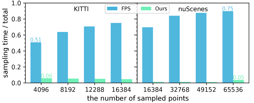
Although remarkable progress has been made in sampling, it is hard to balance the efficiency and effectiveness when it comes to large-scale point clouds, especially for the first downsampling layer. For the sake of higher performance, FPS is the primary method used in many point cloud tasks such as detection [35] and segmentation [30]. However, it takes up to half the inference time when dealing with $10^{5}$ points as shown in Figure 1. And for $10^{6}$ points, the output of a 32-beam LiDAR is infeasible due to its quadratic complexity and iterative algorithm. Therefore, low-latency random point sampling (RPS) is adopted in scenarios where efficiency is critical but suffers from low sampling quality. The learning-based approaches cannot be used in the first downsampling layer due to the lack of sufficient features and the huge sampling probability tensor.

To tackle this problem, we first explore how FPS can benefit the task network to achieve better final performance and then design a more economical algorithm to approximate it. By comparing various algorithms, we discover that the even spacing between points in the subset is the key to the success of FPS, rather than the uniform density of points presented in previous work[30, 31], as inverse density sampling [28] (IDS) also results in poor performance. The uniform distance protects the points in the subset from scattering and clustering with each other, making it less messy (see Section 4.6). This feature allows the geometric information of the original scene to be preserved as much as possible, which is important for downstream detection and segmentation tasks that more focus on shapes. It can be imagined that if we can obtain this property in an efficient way, the performance should be close to FPS. And fortunately, the grid naturally satisfies that because the distance between cells in the grid is constant.

Given the observation mentioned above, we design an adaptive voxel-guided point sampler that hierarchically selects points closest to their grid centers. Our approach has linear time complexity, can be run in parallel, and is both permutation invariant and deterministic. In summary, our main contributions are as follows:

• We revisit several existing sampling techniques and reveal that the key to achieving high-quality sampling is to obtain a uniformly distributed subset.

• Our proposed HAVSampler has a linear time complexity and is parallelizable, making it suitable for real-time applications. Additionally, it is easy to integrate into existing models, making them run up to 5$\times$ faster.

• Our experimental results on various datasets and tasks demonstrate that our method is comparable to or even better than the state-of-the-art method FPS at $10^{2}\sim 10^{4}\times$ faster. This breaks the efficiency bottleneck when using point-based models in large point clouds.

2 Related Work

Point-based Neural Architectures

aim to learn permutation invariant features from unordered point clouds. Serving as feature extractors, point-based models are widely adopted in many downstream tasks, i.e., point cloud detection [5, 35, 47, 49], motion segmentation [38], tracking [52, 40] and registration [1]. The pioneering work PointNet [30] proposes using pointwise MLPs and max pooling to extract robust global features. Succeeding work PointNet++ [31] designs a canonical paradigm that hierarchically samples subsets, groups neighboring points and aggregates contexts to obtain local features. Due to the success of this paradigm, most of the following works keep this process, such as pointwise models [32, 24], graph-based method [43, 16, 50, 41], point convolution [42, 21, 22] and recent transformer-based methods [10, 51]. Obviously, as a first step, sampling has a significant impact on the performance of following feature extraction and task-specific network. This work benefits point cloud applications by presenting an effective and efficient sampling strategy.

Learning-free Point Cloud Samplers

can be used for filtering, pre-processing or as a basic component of point-based networks. RPS [15, 33, 36] is mainly adopted in large-scale point cloud or real-time applications attributed to its high efficiency. IDS [14, 45] tends to probabilistically select the points with lower densities in order to preserve sparse points. Normal space sampling [8] can preserve the edge of point clouds well. Random voxel sampling (RVS) divides points into voxels with a fixed grid and preserves the centroid of the voxels. As one of the most advanced samplers, FPS  [30, 31] is the first choice for many state-of-the-art models. It iteratively selects the point furthest away from the sampled point and updates subset, providing more complete scene coverage. Subsequent works enhance FPS by considering features [47], density [28, 23] and semantic [5].

Although great progress has been made in this area, the trade-off between latency and performance is still a challenge. For object-level point clouds, FPS is the best choice to minimize performance degradation caused by sampling. When confronted with scene-level points, its latency is non-negligible and even dominant, making it unacceptable. Some works [19, 49] attempt to alleviate this computationally inefficient problem by sorting points or dividing scenes into partitions. However, they do not change the mechanics of the sequential FPS and still cannot be executed in parallel. While employing RPS [15] can significantly reduce time consumption, it has a poor performance. Because RPS misses most of the points in the sparse region, it does not capture enough information. IDS [28, 45] can preserve sparse points but conducts time-consuming k-nearest neighbor (KNN) to estimate density. Efficient voxel sampling can smooth uneven density, but the performance is also not ideal. This work solves this difficult balance that hinders the use of point-based networks in many applications.

Learnable Point Cloud Samplers.

Recent research has explored how to adaptively sample the points that are critical for downstream tasks in a learnable way to improve performance. Some works elaborately enhance learning-free sampler with learnable weights [49, 23, 27] or task-oriented loss [6]. Some methods [9, 18] generate subsets directly from MLPs. Others [46, 20] predict a probability matrix with shape of target number $\times$ source number, and make sampling step differentiable by Gumbel-Softmax trick.

However, learnable fashion is not suitable for us. Careful initialisation [20] of these samplers is required, otherwise all points are invisible to subsequent networks at the early training. And the huge probability matrix will occupy all memories when intake large-scale point cloud. More importantly, we want to address the latency/performance trade-off, especially for first-layer sampling in large point clouds. But we lack sufficient features to sample from the source because we sample exactly for extracting finer features.

Figure 2: Illustration of the overall architecture. HAVSampler contains k layers with different voxel sizes, each consisting of an adaptive voxel searching (AVS) module (see Section 3.2) and center-closest selection strategy (see Section 3.3). The leftmost is the original point cloud of a car. The point cloud on the rightmost side is the result of sampling. We show a 2D slice of a car for easier understanding.

3 HAVSampler

We first formulate point sampler and revisit previous work to explore the key for sampling. Next, we describe the overall design of HAVSampler, including the center-closest sampling strategy and adaptive voxel searching module.

3.1 Problem Formulation and Revisiting Study

Point sampling is an essential component of point cloud reasoning, combined with grouping and aggregation to form a basic block. It progressively downsamples source points to build deeper networks and acts as a group center to aggregate local features. For a given set of source points $\mathcal{P}=\{\mathbf{p}_{i}\in\mathbb{R}^{3}\}_{i=1}^{n}$, where each point consists of three coordinates, the point sampler $S$ is expected to extract a subset $\mathcal{P}_{s}=\{\mathbf{p}_{j}\in\mathbb{R}^{3}\}_{j=1}^{m}$ from $\mathcal{P}$. The low-quality sampled result will damage the following feature extractor and block all the other downstream task heads. Therefore, we aim to design an efficient yet powerful sampler for the real-time application of large-scale point clouds.

We revisit the superior FPS and make an in-depth qualitative analysis to find what property makes it stronger. FPS divides the source set $\mathcal{P}$ into two subsets, unselected points $\mathcal{P}_{us}$ and selected points $\mathcal{P}_{s}$. In the beginning, a point is selected at random from the source set to initialize the selected set, and the rest of the source points are considered to be the unselected part. Next step, the point-to-set distance $d_{k}=\min{\left\{\lVert\mathbf{p}_{k}-\mathbf{p}_{j}\rVert\mid\mathbf{p}_{j}\in\mathcal{P}_{s}\right\}}$ is calculated for each unselected point $\mathbf{p}_{k}\in\mathcal{P}_{us}$ to the selected set $\mathcal{P}_{s}$, and the point with the furthest distance is transferred from the unselected set to the selected set. The above procedure is repeated until the selected subset contains enough $m$ points. Let $\mathcal{P}_{us}^{(i)}$ denote the unselected set at i-th iteration, then $\mathcal{P}_{s}$ can be formulated as

$$\mathcal{P}_{s} =\left\{\mathop{\textrm{argmax}}\limits_{\mathbf{p_{k}}}\left\{d_{k}\mid\mathbf{p}_{k}\in\mathcal{P}_{us}^{(i)}\right\}\right\}_{i=1}^{m}.$$ (1)

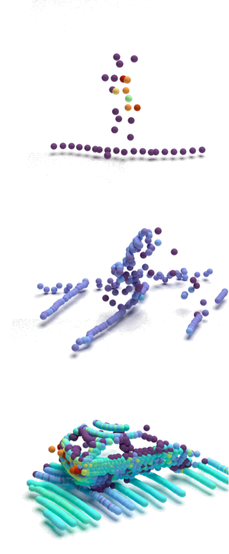
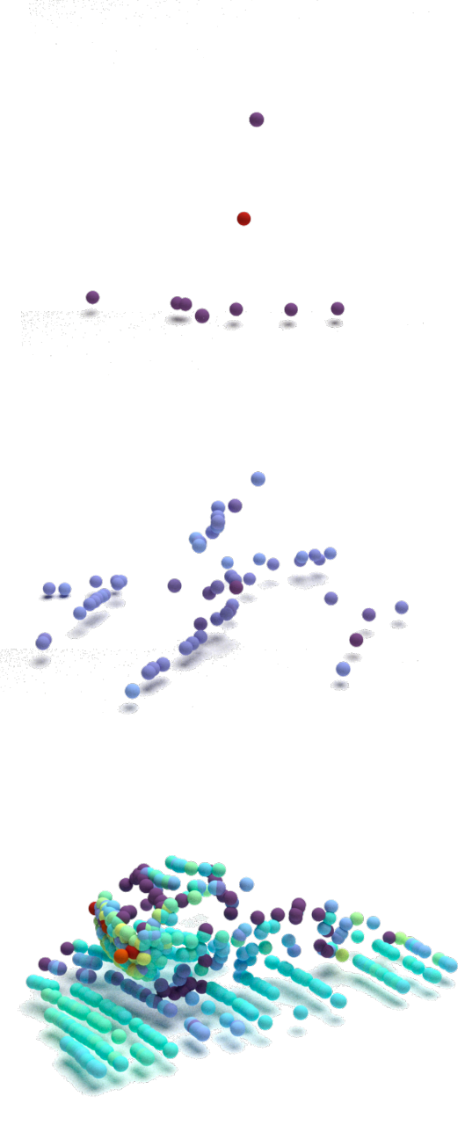
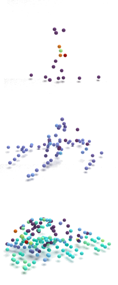
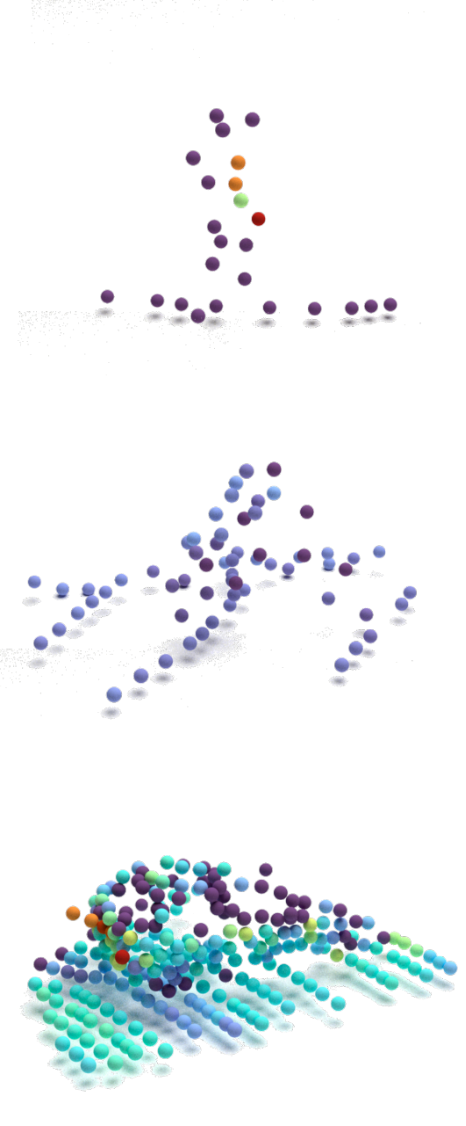
Since we select the furthest points in $\mathcal{P}$ to form $\mathcal{P}_{s}$ by Eq.1, the distances among points in the subset $\mathcal{P}_{s}$ have a lower bound (see supplementary materials for proof), which can be seen in Figure 3. Besides, the point spacing of FPS results has a higher mean value. Larger mean spacing means more scattered sampling results and wider coverage, which maintains a more complete geometry of the raw scene. This complete geometry is critical for the performance of detection and segmentation. And RVS has a similar distribution to FPS, except for a smaller lower bound. In contrast, the spacing distribution of the points in RPS results mostly falls in smaller values, making sampled points cluster together and breaking the raw scene.

Overall, more scattered sampling leads to higher performance. If a similar spacing distribution of points in the subset could be achieved in a more efficient way, we can guess that it would have the same high performance as FPS. Fortunately, the spacing between the grids is naturally constant. As shown in Figure 3, grid-based RVS has a more even spacing than RPS.

Figure 3: The distance distributions of points in different sampled subsets. The red line marks the minimum spacing of FPS results.

3.2 Voxel-guided Sampling

Inspired by the above analysis, we design an efficient voxel-guided sampler with even point spacing and high quality. Since point clouds scanned in 3D space are very sparse  with typically only 0.1% of the voxels containing points [25], we use a sparse approach to voxelize the point cloud to reduce overhead. After that, we select one point from each non-empty voxel to form the final result.

(a) average

(b) random

(c) centre

(d) center-closest

Figure 4: Comparison of different point selections. Deep and light blue grids indicate non-empty and empty voxels, respectively. Black dots is grid center. Orange circles highlights the selections.

Sparse Voxelization via Voxel-Hashing.

Formally, for a given input point cloud $\mathcal{P}$, expected sampling number $m$ and voxel size $\mathbf{v}=\left(v_{x},v_{y},v_{z}\right)$, we compute the voxel coordinate $\mathbf{g}_{i}$ for each $\mathbf{p}_{i}=\left(x_{i},y_{i},z_{i}\right)\in\mathcal{P}$ as shown in

$$\mathbf{g}_{i}=\left(u,v,w\right)=\left(\lfloor\frac{x_{i}}{v_{x}}\rfloor,\lfloor\frac{y_{i}}{v_{y}}\rfloor,\lfloor\frac{z_{i}}{v_{z}}\rfloor\right).$$ (2)

After that, we need to find the all non-empty voxels to perform sampling. Some works [39] filter out the duplicate elements in $\{\mathbf{g}_{i}\}$ by the unique operation that with a computational complexity of at least $\mathcal{O}(n\log{n})$. Instead of unique operation, we use hashtable $\mathcal{T}$ to implement the integer coordinates de-duplication with linear complexity. For each $\mathbf{p}_{i}$, it fills the table at slot $c_{i}=\textrm{hash}\left(\mathbf{g}_{i}\right)$. Finally we obtain the all non-empty voxels by traversing the $\mathcal{T}$. Note that the above steps can be executed in parallel.

Center-closest Point Sampling.

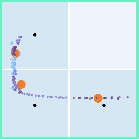
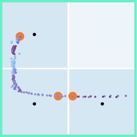
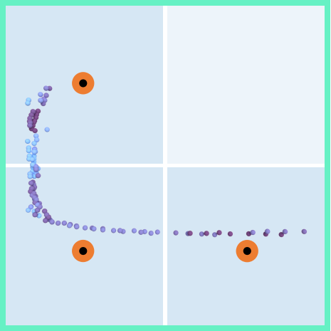
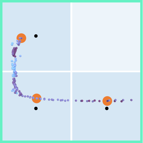
One problem remains to be solved here: which point in a non-empty voxel should we choose to represent that voxel? Previous works mainly select the average, center, or random points of a voxel, as shown in Figure 4. We observe three drawbacks to these: (1) the average value or the center of the voxel is a fake point that does not belong to the original set; (2) random selection or average points will reduce the spacing between points; (3) the use of centers introduces quantization errors.

Taking these three aspects into account, we propose selecting the point closest to the voxel center as the representative. Formally, we extend $\mathcal{T}$ to store pairs of point index and the distance $(i,d_{i})$. For each $\mathbf{p}_{i}\in\mathcal{P}$, its distance to corresponding voxel centre is computed by $d_{i}=\lVert\mathbf{p}_{i}-\mathbf{v}\odot\left(\mathbf{g}_{i}+0.5\right)\rVert$, where $\odot$ is element-wise multiplication. To finger out the closest points, we update $\mathcal{T}(c_{i})$ with $(i,d_{i})$ pair if $d_{i}$ is smaller than the existing distance value at slot $c_{i}$, which means $\mathbf{p}_{i}$ is closer to the center than other points in the same voxel. As illustrated in Figure 4, the points sampled by our strategy are included in the source set and have no quantification errors. Besides, by being closest to the grid center, the spacing between sampled points is scattered as much as possible. Therefore, our strategy can approximate the point distribution of FPS in an efficient manner and achieves high performance.

Figure 5: Statistical results on KITTI dataset. (a) Distribution of optimum voxel size when sampling 4096 points. (b) Red curve shows the distribution of the number of non-empty voxels, i.e., the number of sampled points, when fixing the voxel size to $[0.34,0.34,0.30]$ m, mean of the optimum voxel in (a); The orange curve is the normalized area under the red curve.

3.3 Adaptive Voxel Initialization Strategy

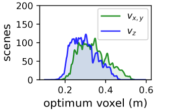
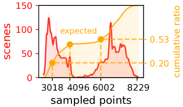
Although we can extract a subset with a scattered point distribution, there is still a hyper-parameter, the voxel size $\mathbf{v}$, that needs to be tuned. Most previous works [44, 17, 48] use a fixed voxel size across different scenes. However, the scale of different point clouds can vary greatly, resulting in too many or too few non-empty voxels and sampled points. As shown in Figure 5, the most suitable voxel size, i.e., the number of non-empty voxels matches the expected sampling number, can widely range between 0.2$\sim$0.5 m for different scenes. Sampling with the mean of the optimal voxel, Figure 5 shows that there will be about 20% scenes with 25% undersampling rate and up to 50% scenes with 50% oversampling rate. Therefore, the sampled points need to be resampled or cut off, resulting in subsets containing redundant points or missing information.

We recognize the need to select the voxel size for each scene adaptively. This strategy helps to retain more of the information present in the raw scene. Typically, the smaller the voxel size, the more non-empty voxels in a scene, so more points are sampled. Thanks to this monotonically decreasing property, we can determine the most suitable voxel size for a given scene by performing a binary search. To this end, we design an adaptive voxel searching (AVS) module to find a suitable voxel size $\mathbf{v}=\textrm{AVS}(\mathcal{P},m)$ for the given point cloud $\mathcal{P}$ and expected sampling number $m$. we compute the number of non-empty voxels $m_{s}$ for a given searched voxel size $\mathbf{v_{s}}$ by implementing a voxel counter $m_{s}=\textrm{Cnt}\left(\mathcal{P},\mathbf{v_{s}}\right)$ in a voxel-hashing manner similar to Section 3.2. During the binary search, the output voxel size will be updated iteratively until the number of non-empty voxels falls into the interval $[m,(1+\sigma)m]$ with tolerance factor $\sigma$, or the iteration times exceeds $t_{max}$.

3.4 Hierarchical Paradigm

So far, we can obtain high-quality sampling results with the above components. However, only sampling with a single granularity lacks the ability to capture various scene structures differently. For example, some simple geometries like floors and walls only require coarse-grained sampling, whereas pedestrians and cyclists require finer grain.

Therefore, we introduce a hierarchical point cloud sampling framework that samples the scene at different scales from coarse to fine. The overall pipeline is illustrated in Figure 2. Our framework has k layers, each consisting of an adaptive voxel searching module AVS and center-closest point sampling S. For layer $\ell$, we obtain $\ell$-th subset by

$$\mathcal{P}^{\prime}_{\ell}=\textrm{S}\left(\mathcal{P}_{\ell},\textrm{AVS}\left(\mathcal{P}_{\ell},m_{\ell}\right)\right),$$ (3)

where $\mathcal{P}_{\ell}$ and $m_{\ell}$ are the input and sampling number of $\ell$ layer, respectively. Then we mask the points in $\mathcal{P}_{\ell}$ as sampled state with $\mathcal{P}^{\prime}_{\ell}$ to form the input of next layer $\mathcal{P}_{\ell+1}$. As for $m_{\ell}$, we set it to be $4m_{\ell-1}$ and satisfy $m=\sum_{\ell=1}^{k}{m_{\ell}}$. Finally, we gather all subsets $\mathcal{P}^{\prime}_{\ell}$ to generate the output $\mathcal{P}^{\prime}$.

4 Experiments

We conduct extensive experiments for the proposed HAVSampler in this section. We first introduce the experimental settings in Section 4.1. Then the comparison of runtime shown in Section 4.2 indicates the efficiency of our method. We further evaluate the proposed method on various tasks, including large-scale detection (Section 4.3) and segmentation (Section 4.4) in both indoor and outdoor scenes, to show the effectiveness. Finally, we conduct an ablation study in Section 4.5 to evaluate each component.

4.1 Experimental Settings

We compare outdoor point cloud object detection based on the OpenPCDet [39] toolbox. For scene segmentation and indoor object detection, we adapt our sampler for the official implementation of each model. All experiments are run on an i7-6700 CPU and a single RTX 2080Ti GPU.

Datasets.

The large-scale KITTI [13] and nuscenes [4] datasets are used for efficiency comparison and outdoor point cloud object detection. And SUN RGB-D [37] dataset is used to compare point cloud object detection in indoor scenes. We conduct outdoor and indoor scene semantic segmentation experiments based on SemanticKITTI [3] dataset and S3DIS [2] dataset, respectively. The splits, setup and pre-processing of each dataset follow previous work.

Implementation Details.

For all experiments except ablation study, we employ a 2-layer structure for the proposed HAVSampler. For AVS, the tolerance $\sigma$ and max iteration times $t_{max}$ are set to $0.05$ and 20, respectively. We implement parallel voxel-hashing on the GPU via cuHash [12].

4.2 Efficiency

In this section, we empirically compare the proposed HAVSampler with RPS, RVS and FPS to get an intuitive feel for the efficiency of our method.

Complexity Analysis

We first analyze the complexity of these methods and summarise them in Table 1. There is no doubt that RPS has the lowest time and space complexity. Conversely, the best FPS has the highest time complexity. For ours, sparse voxelization based on voxel-hashing has $\mathcal{O}\left(N\right)$ complexity. The center-closest sampling strategy accesses and updates non-empty voxels individually for each point with $\mathcal{O}\left(1\right)$ complexity. Similarly, we takes $\mathcal{O}\left(N\right)$ to perform voxel counter $\textrm{Cnt}(\cdot,\cdot)$ for one iteration in AVS. While it takes $\mathcal{O}\left(\log{N}\right)$ iterations to find a certain value by binary search, we only need at most $\lceil\log{\frac{1}{\sigma}}\rceil$ iterations to converge within a given tolerance $\sigma$. Summarily, our method has a time complexity of $\mathcal{O}(N)$.

Method	RPS	RVS	FPS	Ours
Point	$\mathcal{O}\left(N\right)$	$\mathcal{O}\left(N\right)$	$\mathcal{O}\left(N^{2}\right)$	$\mathcal{O}\left(N\right)$
Space	$\mathcal{O}\left(1\right)$	$\mathcal{O}\left(N\right)$	$\mathcal{O}\left(N\right)$	$\mathcal{O}\left(N\right)$

Table 1: The time and space complexity of different methods. We sample from N points with a typical ratio of 4.

Dataset	Detector		Sampler		Performance				Latency (ms)
			train	test	Car AP@R11		Car AP@R40		batch size=1		batch size=8
KITTI val set	PointRCNN [35]	*	FPS	FPS	79.39		82.96		119.9		75.6
			FPS	RPS	76.89	-1.24	77.27	-3.21	94.9	-20.9%	70.0	-7.4%
			FPS	ours	79.21	-0.18	82.96	0.00	95.1	-20.7%	71.8	-5.7%
	PV-RCNN [34]	*	FPS	FPS	79.09		82.68		117.4		68.5
			FPS	RPS	76.89	-2.20	77.28	-5.37	88.0	-25.0%	47.7	-30.4%
			FPS	ours	79.98	-0.11	82.53	-0.12	90.6	-22.8%	48.4	-29.3%
	3DSSD [47]	*	FPS	FPS	84.14		84.54		84.9		35.3
			FPS	RPS	78.08	-6.06	80.03	-4.51	47.8	-36.2%	31.7	-10.2%
			FPS	ours	84.26	+0.12	84.79	+0.25	49.1	-34.5%	31.9	-9.5%
	SASA [5]	*	FPS	FPS	84.20		84.67		63.4		23.0
			FPS	RPS	77.46	-6.73	77.76	-6.90	35.9	-43.4%	19.8	-14.0%
			FPS	ours	84.54	+0.34	85.13	+0.47	39.1	-38.3%	20.2	-12.2%
			ours	ours	84.42	+0.22	84.81	+0.15	39.1	-38.3%	20.2	-12.2%
	IA-SSD [49]	*	FPS	FPS	79.22		83.02		46.4		13.8
			FPS	RPS	77.29	-1.93	77.59	-5.44	19.5	-58.0%	10.7	-22.4%
			FPS	ours	79.36	+0.14	83.21	+0.19	20.1	-56.7%	10.8	-22.0%
			ours	ours	84.27	+5.05	85.04	+2.02	20.1	-56.7%	10.8	-22.0%
					NDS		mAP		batch size=1		batch size=4
nuScenes val set	SASA [5]	*	FPS	FPS	58.55		41.24		500.9		194.2
			FPS	RPS	54.59	-3.96	34.51	-6.73	164.0	-67.3%	109.3	-43.7%
			FPS	ours	58.24	-0.31	40.67	-0.57	165.1	-67.1%	109.2	-43.8%
			ours	ours	58.58	+0.03	41.28	+0.04	165.1	-67.1%	109.2	-43.8%
	IA-SSD [49]	*	FPS	FPS	54.42		37.01		439.0		130.7
			FPS	RPS	50.76	-3.66	31.23	-5.66	85.1	-80.6%	45.6	-65.1%
			FPS	ours	54.00	-0.42	36.22	-0.67	85.0	-80.7%	45.7	-65.0%
			ours	ours	55.04	+0.62	37.01	+0.12	85.0	-80.7%	45.7	-65.0%

Table 2: Performance of outdoor 3D object detection. The effect of samplers is evaluated by replacing the first layer sampler of the original models. We report the 3D AP calculated by both 11 and 40 recall positions for KITTI. For nuScenes, we follow the standard protocol [4] by reporting NDS and mAP. Besides, the latency measured with test with different batch size is also shown. *: the original configuration.

Latency Comparison

Figure 6: We conduct 3 groups of experiments with different scale inputs, (left) small scale with $2^{14}$ points, (mid) medium scale with $2^{16}$ points and (right) $2^{18}$ points for large scale. In each group, the point cloud is downsampled by 3 steps with a ratio of 2 at each step. Green solid line indicates ours.

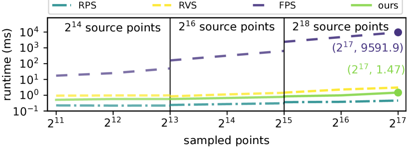
Figure 6 shows the results of our latency comparison. We conduct experiments on 3 different input scales to compare the runtimes in different application scenarios: (1) small-scale scenarios with $2^{14}$ points such as the KITTI dataset; (2) $2^{16}$-point medium-sized scenes like the nuSCenes dataset; (3) large-scale $2^{18}$ points, the same order of magnitude as the output of 64-beam LiDAR. And all the methods run in parallel on the GPU.

Unsurprisingly, RPS is the fastest method, while the heavy FPS has the highest latency due to the quadratic complexity and difficulty of parallelism. FPS takes more than 9 seconds to sample from $2^{18}$ points to $2^{17}$ points. This means that it cannot be used to directly process the original point cloud output from LiDAR. It can be noticed that for all experimental configurations, our method can run within 1.47ms. Moreover, our HAVSampler is even fast than RVS, which is also based on the voxels. Experimental results show that our algorithm has efficiency on the same level as RPS and RVS, and is $10^{2}$ to $10^{4}$ times faster than FPS.

4.3 Point Cloud Object Detection

In this section, We evaluate the impact of the proposed HAVSampler on 3D object detection task. For a fair comparison, we test all detectors on the same platform.

Detector		Sampler		mAP@0.5	bed	tables	sofa	chair	toilet	desk	dresser	nightstand	bookshelf	bathtub
		train	test
VoteNet [29]	*	FPS	FPS	33.32	47.98	19.44	42.35	53.78	63.97	5.29	15.7	35.86	4.54	45.24
		FPS	ours	32.82	46.87	20.25	42.93	53.17	56.84	5.12	14.93	37.18	4.89	46.04
		improve		-0.50	-1.12	+0.81	+0.58	-0.61	-6.12	-0.17	-0.80	+1.32	+0.35	+0.81
3DETR [26]	*	FPS	FPS	30.73	48.13	18.23	40.74	44.65	66.89	7.93	12.33	31.13	4.96	32.32
		FPS	ours	32.01	51.50	20.00	39.17	45.61	64.48	5.90	14.67	34.52	5.66	38.88
		improve		+1.28	+3.37	+1.77	-1.57	+0.96	-2.41	-2.03	+2.34	+3.39	+0.70	+6.56

Table 3: Performance of indoor 3D object detection on SUN RGN-D dataset. We replace the first layer sampler of the original models. The reported mAP is calculated at the more strict IoU threshold of 0.5. *: the original configuration.

Outdoor Scenes

We first evaluate our HAVSampler on KITTI val set and report the results in Table 2. To compare the effect of samplers on detector performance, we replace the first layer of samplers in the original model with different sampling methods. Comparing the first and second rows in Table 2, When we directly replace the FPS with RPS in models and test without retraining, the 3D AP at both R11 and R40 drops significantly for all models. Especially, SASA has a performance degradation with 6.73 AP and 6.90 AP at R11 and R40, respectively. However, we observe that the detection performance is unchanged or even slightly higher than FPS when tested directly test with our HAVSampler. It should be noted that the follow-up networks of samplers are sensitive to the distribution of sampled points after training, so performance will commonly degrade when tested with different samplers. The similar performance between our method and FPS means that the proposed HAVSampler has a distribution close to that of FPS, which verifies our observations in Section 3.1. In addition, our method can greatly reduce detector runtimes by up to 56.7%, meaning that our method is highly efficient. We also retrain two lightweight models, SASA and IA-SSD, with our HAVSampler. Comparing the first and last rows of them, the performance improved after retraining. Most surprisingly, our approach makes the IA-SSD improve by a large margin of 5.05% AP@R11 and can infer at a speed of 50 Hz.

We also experiment on larger scenes dataset, nuScenes, and report the results at the bottom of Table 2. With similar results on KITTI dataset, RPS has the worst performance. Our method yields a slight performance gain after retraining. Notably, the efficiency advantage of our method is even more remarkable when dealing with larger point clouds, saving 80.7% of time consumption.

In summary, our method can be adapted to large-scale outdoor 3D object detection tasks. As well as saving time, HAVSampler has the potential to boost performance.

Indoor Scenes

Instead of LiDAR, indoor data sets are captured by RGB-D cameras. We evaluated our method on the SUN RGB-D dataset to verify its applicability to different sensor data and show results in Table 3. We report the more strict mAP calculated at IoU threshold of 0.5. In VoteNet [29], our sampling strategy has a performance degradation of 0.5 mAP. However, an increase of 1.28 mAP is obtained for transformer-based 3D detector 3DETR [26]. This subsection manifests again that our samplers have a similar performance with FPS on detection tasks.

Recall Analysis

Method	RPS	RVS	FPS	Ours
Point recall	24.99%	19.87%	18.16%	18.56%
Instance recall	98.18%	99.90%	99.94%	99.96%

Table 4: Recall analysis on KITTI dataset.

We downsampled the points to 1/4 of the input and analyzed the recall of different samplers on the KITTI dataset. Point recall is the ratio of points belonging to foreground objects existed in the subset. Instance recall refers to the percentage of instances that contain more than 1 point in the subset. Although RPS retains the most foreground points, it has the lowest instance recall due to the loss of distant points, which can be visualized in Figure 7. Compared to FPS, our method has a higher point recall while still keeping more instances after downsampling, which is important for detection tasks.

4.4 Point Cloud Scene Segmentation

	Dataset	Model		Sampler		mIoU
				train	test
Outdoor	SemanticKITTI [3] sequence 8	RandLA-Net [15]	*	RPS	RPS	50.0
				RPS	ours	51.0	+1.0
				ours	ours	54.1	+4.1
		BAAF-Net [33]	*	FPS	FPS	48.6
				FPS	ours	49.2	+0.6
				ours	ours	51.7	+3.1
		BAF-LAC [36]	*	RPS	RPS	47.8
				RPS	ours	47.6	-0.2
				ours	ours	48.0	+0.2
Indoor	S3DIS [2] 6-fold CV	RandLA-Net [15]	*	RPS	RPS	70.1
				RPS	ours	70.3	+0.3
		BAAF-Net [33]	*	FPS	FPS	72.1
				FPS	ours	72.0	-0.1
		SCF-Net [11]	*	RPS	RPS	71.6
				RPS	ours	71.7	+0.1

Table 5: Performance of both outdoor and indoor point cloud scene segmentation. We report the mean IoU on SemanticKITTI val set. As for S3DIS, we compute the mean IoU by the 6-fold cross validation. *: the original configuration.

The scene segmentation task densely predicts per-point semantics for large-scale point clouds, requiring greater efficiency and sampling quality than detection.

Outdoor Scenes

The results at the top of table 5 show the advantages of our method in scene segmentation. Our sampling strategy outperforms both RPS and FPS by a large margin, improving by 4.1% and 3.1% mIoU after retraining, respectively. For BAF-LAC, however, there is no noticeable change compared to RPS. We guess it is mainly because the backward attention fusing mechanism in BAF-LAC [36] complements the points lost by RPS with skip connections.

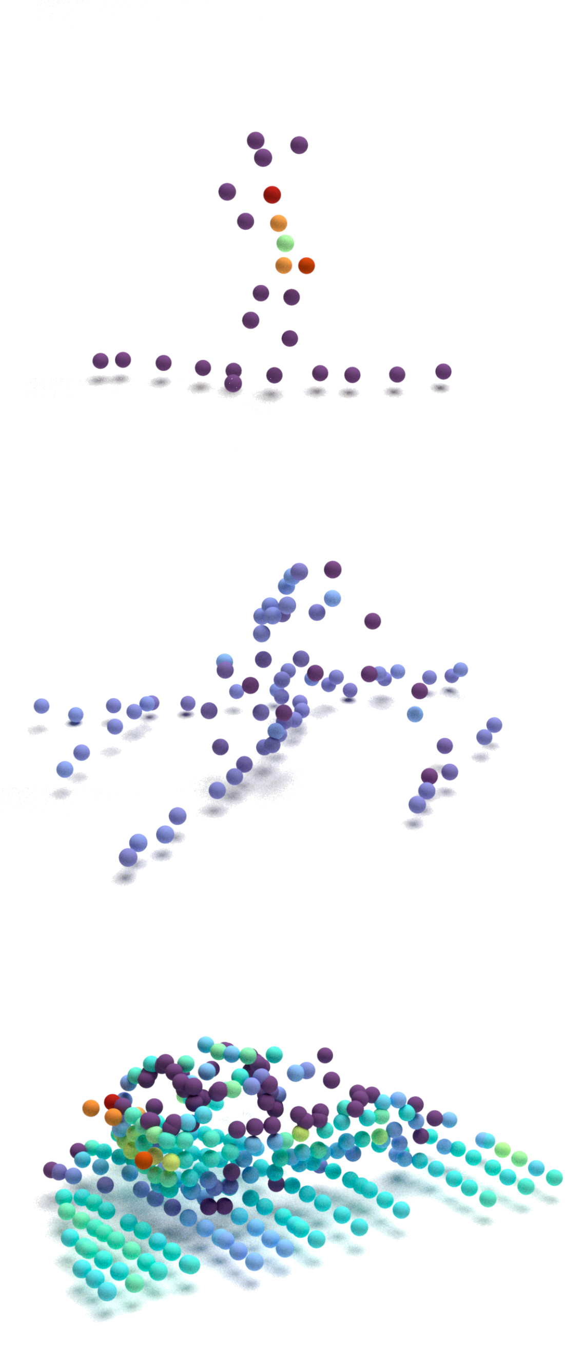
Car        Cyclist      Pedestrian

(a) source

(b) RPS

(c) RVS

(d) FPS

(e) Ours

Figure 7: Examples of different sampling results. From top to bottom: a near car, a medium distance cyclist, a distant pedestrian.

Indoor Scenes

The rest of Table 5 shows the indoor segmentation results. I find that our samplers have less performance improvement indoors. In all models, it brings no more than 0.3% mIoU change. We suspect that the main reason for this is that RGB-D captures denser point clouds indoors than outdoor LiDAR. So there has not been much change in either the replacement of FPS or RPS.

4.5 Ablation Study

#	L	Point section strategy				Voxel		Moderate Car
		ME	RA	CE	CC	Fix	Ada	AP@R11	AP@R40
1	1	$\checkmark$				$\checkmark$		79.29	83.04
	1	$\checkmark$					$\checkmark$	83.81	84.49
2	1		$\checkmark$			$\checkmark$		79.03	82.69
	1		$\checkmark$				$\checkmark$	79.45	83.24
3	1			$\checkmark$		$\checkmark$		79.27	82.99
	1			$\checkmark$			$\checkmark$	83.81	84.49
4	1				$\checkmark$	$\checkmark$		79.24	82.93
	1				$\checkmark$		$\checkmark$	84.08	84.67
5	2				$\checkmark$		$\checkmark$	84.27	85.04
	3				$\checkmark$		$\checkmark$	79.20	83.04

Table 6: Effects of different strategies of layer, point selection and voxel initialisation for HAVSampler. ME: mean. RA: random. CE: centre. CC: center-closest. Fix: Fixed voxel size. Ada: Adaptive voxel size. The red row is baseline RVS. The row in blue is the best configuration for the proposed method.

We use IA-SSD detector and KITTI dataset for quick experiments. The results of car detection are shown in Table 6. From groups 1-4, we can see that the random selection of a representative point in voxels has the worst performance. Besides, when using adaptive voxels, our most center-closest point selection helps the detector to obtain higher APs. For all point selection strategies, adaptive voxels bring major performance improvements. Group 5 investigates how the number of layers in our architecture affects performance. The experimental results indicate that a 2-layer structure can achieve the best performance.

4.6 Qualitative Results and Discussion

Figure 7 shows examples of point clouds subset from different samplers. In line with Table 4, RPS retains most of the points close to the sensor, but loses most points further away. In contrast, RVS can prevent the distant points from being abandoned but has messy sampling results at the near place. From the last two columns, it can be observed that both FPS and our HAVSampler well deal with the point cloud at all distances and preserve the skeleton of source point clouds when downsampling.

5 Limitations

Although the performance of efficient HAVSampler is competitive with or even higher than the state-of-the-art FPS on object detection and scene segmentation. We find that compared to indoor RGB-D point clouds, HAVSampler performs better for outdoor LiDAR point clouds. In addition, our experiments on point cloud classification and partition segmentation show that there is a counter-intuitive drop in performance when replacing the FPS with ours, which can be seen in the supplementary material. But this performance degradation is still much smaller than using RPS. However, the sampler latency in these object-level tasks is ignorable and so is not a concern for us.

6 Conclusion

We present HAVSampler, an highly efficient yet powerful sampler for real-time applications in large-scale point clouds. We reveal that evenly spacing the points in the subset is crucial for optimizing the performance of downstream tasks Based on this conclusion, our design of grid-guided paradigm, adaptive voxelization, and hierarchical architecture results in outstanding performance while reducing inference time by 20-80%. This breakthrough in efficiency addresses the bottleneck of the sampling step in real-time applications. We release our source code and hope that it can serve as a solid component to inspire and encourage the point cloud learning community.

References

- [1] Yasuhiro Aoki, Hunter Goforth, Rangaprasad Arun Srivatsan, and Simon Lucey. Pointnetlk: Robust & efficient point cloud registration using pointnet. In Proceedings of the IEEE/CVF conference on computer vision and pattern recognition, pages 7163–7172, 2019.
- [2] Iro Armeni, Sasha Sax, Amir R Zamir, and Silvio Savarese. Joint 2d-3d-semantic data for indoor scene understanding. arXiv preprint arXiv:1702.01105, 2017.
- [3] Jens Behley, Martin Garbade, Andres Milioto, Jan Quenzel, Sven Behnke, Cyrill Stachniss, and Jurgen Gall. Semantickitti: A dataset for semantic scene understanding of lidar sequences. In Proceedings of the IEEE/CVF international conference on computer vision, pages 9297–9307, 2019.
- [4] Holger Caesar, Varun Bankiti, Alex H Lang, Sourabh Vora, Venice Erin Liong, Qiang Xu, Anush Krishnan, Yu Pan, Giancarlo Baldan, and Oscar Beijbom. nuscenes: A multimodal dataset for autonomous driving. In Proceedings of the IEEE/CVF conference on computer vision and pattern recognition, pages 11621–11631, 2020.
- [5] Chen Chen, Zhe Chen, Jing Zhang, and Dacheng Tao. Sasa: Semantics-augmented set abstraction for point-based 3d object detection. In Proceedings of the AAAI Conference on Artificial Intelligence, volume 36, pages 221–229, 2022.
- [6] Huixian Cheng, XianFeng Han, Hang Jiang, Dehong He, and Guoqiang Xiao. Pcb-randnet: Rethinking random sampling for lidar semantic segmentation in autonomous driving scene. arXiv preprint arXiv:2209.13797, 2022.
- [7] Ta-Ying Cheng, Qingyong Hu, Qian Xie, Niki Trigoni, and Andrew Markham. Meta-sampler: Almost-universal yet task-oriented sampling for point clouds. In Computer Vision–ECCV 2022: 17th European Conference, Tel Aviv, Israel, October 23–27, 2022, Proceedings, Part II, pages 694–710. Springer, 2022.
- [8] Yago Diez, Joan Martí, and Joaquim Salvi. Hierarchical normal space sampling to speed up point cloud coarse matching. Pattern Recognition Letters, 33(16):2127–2133, 2012.
- [9] Oren Dovrat, Itai Lang, and Shai Avidan. Learning to sample. In Proceedings of the IEEE/CVF Conference on Computer Vision and Pattern Recognition, pages 2760–2769, 2019.
- [10] Nico Engel, Vasileios Belagiannis, and Klaus Dietmayer. Point transformer. IEEE Access, 9:134826–134840, 2021.
- [11] Siqi Fan, Qiulei Dong, Fenghua Zhu, Yisheng Lv, Peijun Ye, and Fei-Yue Wang. Scf-net: Learning spatial contextual features for large-scale point cloud segmentation. In Proceedings of the IEEE/CVF Conference on Computer Vision and Pattern Recognition, pages 14504–14513, 2021.
- [12] David Farrell. Simplegpuhashtable. https://github.com/nosferalatu/SimpleGPUHashTable, 2020.
- [13] Andreas Geiger, Philip Lenz, and Raquel Urtasun. Are we ready for autonomous driving? the kitti vision benchmark suite. In 2012 IEEE conference on computer vision and pattern recognition, pages 3354–3361. IEEE, 2012.
- [14] Fabian Groh, Patrick Wieschollek, and Hendrik PA Lensch. Flex-convolution: Million-scale point-cloud learning beyond grid-worlds. In Computer Vision–ACCV 2018: 14th Asian Conference on Computer Vision, Perth, Australia, December 2–6, 2018, Revised Selected Papers, Part I 14, pages 105–122. Springer, 2019.
- [15] Qingyong Hu, Bo Yang, Linhai Xie, Stefano Rosa, Yulan Guo, Zhihua Wang, Niki Trigoni, and Andrew Markham. Randla-net: Efficient semantic segmentation of large-scale point clouds. In Proceedings of the IEEE/CVF conference on computer vision and pattern recognition, pages 11108–11117, 2020.
- [16] Loic Landrieu and Martin Simonovsky. Large-scale point cloud semantic segmentation with superpoint graphs. In Proceedings of the IEEE conference on computer vision and pattern recognition, pages 4558–4567, 2018.
- [17] Alex H Lang, Sourabh Vora, Holger Caesar, Lubing Zhou, Jiong Yang, and Oscar Beijbom. Pointpillars: Fast encoders for object detection from point clouds. In Proceedings of the IEEE/CVF conference on computer vision and pattern recognition, pages 12697–12705, 2019.
- [18] Itai Lang, Asaf Manor, and Shai Avidan. Samplenet: Differentiable point cloud sampling. In Proceedings of the IEEE/CVF Conference on Computer Vision and Pattern Recognition, pages 7578–7588, 2020.
- [19] Jingtao Li, Jian Zhou, Yan Xiong, Xing Chen, and Chaitali Chakrabarti. An adjustable farthest point sampling method for approximately-sorted point cloud data. In 2022 IEEE Workshop on Signal Processing Systems (SiPS), pages 1–6. IEEE, 2022.
- [20] Luyang Li, Ligang He, Jinjin Gao, and Xie Han. Psnet: Fast data structuring for hierarchical deep learning on point cloud. IEEE Transactions on Circuits and Systems for Video Technology, 32(10):6835–6849, 2022.
- [21] Yangyan Li, Rui Bu, Mingchao Sun, Wei Wu, Xinhan Di, and Baoquan Chen. Pointcnn: Convolution on x-transformed points. Advances in neural information processing systems, 31, 2018.
- [22] Yongcheng Liu, Bin Fan, Shiming Xiang, and Chunhong Pan. Relation-shape convolutional neural network for point cloud analysis. In Proceedings of the IEEE/CVF Conference on Computer Vision and Pattern Recognition (CVPR), June 2019.
- [23] Ze Liu, Zheng Zhang, Yue Cao, Han Hu, and Xin Tong. Group-free 3d object detection via transformers. In Proceedings of the IEEE/CVF International Conference on Computer Vision, pages 2949–2958, 2021.
- [24] Xu Ma, Can Qin, Haoxuan You, Haoxi Ran, and Yun Fu. Rethinking network design and local geometry in point cloud: A simple residual mlp framework. arXiv preprint arXiv:2202.07123, 2022.
- [25] Jiageng Mao, Yujing Xue, Minzhe Niu, Haoyue Bai, Jiashi Feng, Xiaodan Liang, Hang Xu, and Chunjing Xu. Voxel transformer for 3d object detection. In Proceedings of the IEEE/CVF International Conference on Computer Vision (ICCV), pages 3164–3173, October 2021.
- [26] Ishan Misra, Rohit Girdhar, and Armand Joulin. An end-to-end transformer model for 3d object detection. In Proceedings of the IEEE/CVF International Conference on Computer Vision, pages 2906–2917, 2021.
- [27] Ehsan Nezhadarya, Ehsan Taghavi, Ryan Razani, Bingbing Liu, and Jun Luo. Adaptive hierarchical down-sampling for point cloud classification. In Proceedings of the IEEE/CVF Conference on Computer Vision and Pattern Recognition, pages 12956–12964, 2020.
- [28] Jingmei Ning, Feipeng Da, and Shaoyan Gai. Density aware 3d object single stage detector. IEEE Sensors Journal, 21(20):23108–23117, 2021.
- [29] Charles R Qi, Or Litany, Kaiming He, and Leonidas J Guibas. Deep hough voting for 3d object detection in point clouds. In proceedings of the IEEE/CVF International Conference on Computer Vision, pages 9277–9286, 2019.
- [30] Charles R Qi, Hao Su, Kaichun Mo, and Leonidas J Guibas. Pointnet: Deep learning on point sets for 3d classification and segmentation. In Proceedings of the IEEE conference on computer vision and pattern recognition, pages 652–660, 2017.
- [31] Charles Ruizhongtai Qi, Li Yi, Hao Su, and Leonidas J Guibas. Pointnet++: Deep hierarchical feature learning on point sets in a metric space. Advances in neural information processing systems, 30, 2017.
- [32] Guocheng Qian, Yuchen Li, Houwen Peng, Jinjie Mai, Hasan Abed Al Kader Hammoud, Mohamed Elhoseiny, and Bernard Ghanem. Pointnext: Revisiting pointnet++ with improved training and scaling strategies. arXiv preprint arXiv:2206.04670, 2022.
- [33] Shi Qiu, Saeed Anwar, and Nick Barnes. Semantic segmentation for real point cloud scenes via bilateral augmentation and adaptive fusion. In Proceedings of the IEEE/CVF Conference on Computer Vision and Pattern Recognition, pages 1757–1767, 2021.
- [34] Shaoshuai Shi, Chaoxu Guo, Li Jiang, Zhe Wang, Jianping Shi, Xiaogang Wang, and Hongsheng Li. Pv-rcnn: Point-voxel feature set abstraction for 3d object detection. In Proceedings of the IEEE/CVF Conference on Computer Vision and Pattern Recognition, pages 10529–10538, 2020.
- [35] Shaoshuai Shi, Xiaogang Wang, and Hongsheng Li. Pointrcnn: 3d object proposal generation and detection from point cloud. In Proceedings of the IEEE/CVF conference on computer vision and pattern recognition, pages 770–779, 2019.
- [36] Hui Shuai, Xiang Xu, and Qingshan Liu. Backward attentive fusing network with local aggregation classifier for 3d point cloud semantic segmentation. IEEE Transactions on Image Processing, 30:4973–4984, 2021.
- [37] Shuran Song, Samuel P Lichtenberg, and Jianxiong Xiao. Sun rgb-d: A rgb-d scene understanding benchmark suite. In Proceedings of the IEEE conference on computer vision and pattern recognition, pages 567–576, 2015.
- [38] Yuxiang Sun, Weixun Zuo, Huaiyang Huang, Peide Cai, and Ming Liu. Pointmoseg: Sparse tensor-based end-to-end moving-obstacle segmentation in 3-d lidar point clouds for autonomous driving. IEEE Robotics and Automation Letters, 6(2):510–517, 2020.
- [39] OpenPCDet Development Team. Openpcdet: An open-source toolbox for 3d object detection from point clouds. https://github.com/open-mmlab/OpenPCDet, 2020.
- [40] Sukai Wang, Yuxiang Sun, Chengju Liu, and Ming Liu. Pointtracknet: An end-to-end network for 3-d object detection and tracking from point clouds. IEEE Robotics and Automation Letters, 5(2):3206–3212, 2020.
- [41] Yue Wang, Yongbin Sun, Ziwei Liu, Sanjay E Sarma, Michael M Bronstein, and Justin M Solomon. Dynamic graph cnn for learning on point clouds. Acm Transactions On Graphics (tog), 38(5):1–12, 2019.
- [42] Wenxuan Wu, Zhongang Qi, and Li Fuxin. Pointconv: Deep convolutional networks on 3d point clouds. In Proceedings of the IEEE/CVF Conference on Computer Vision and Pattern Recognition (CVPR), June 2019.
- [43] Qiangeng Xu, Xudong Sun, Cho-Ying Wu, Panqu Wang, and Ulrich Neumann. Grid-gcn for fast and scalable point cloud learning. In Proceedings of the IEEE/CVF Conference on Computer Vision and Pattern Recognition, pages 5661–5670, 2020.
- [44] Yan Yan, Yuxing Mao, and Bo Li. Second: Sparsely embedded convolutional detection. Sensors, 18(10):3337, 2018.
- [45] Honghui Yang, Zili Liu, Xiaopei Wu, Wenxiao Wang, Wei Qian, Xiaofei He, and Deng Cai. Graph r-cnn: Towards accurate 3d object detection with semantic-decorated local graph. In Computer Vision–ECCV 2022: 17th European Conference, Tel Aviv, Israel, October 23–27, 2022, Proceedings, Part VIII, pages 662–679. Springer, 2022.
- [46] Jiancheng Yang, Qiang Zhang, Bingbing Ni, Linguo Li, Jinxian Liu, Mengdie Zhou, and Qi Tian. Modeling point clouds with self-attention and gumbel subset sampling. In Proceedings of the IEEE/CVF conference on computer vision and pattern recognition, pages 3323–3332, 2019.
- [47] Zetong Yang, Yanan Sun, Shu Liu, and Jiaya Jia. 3dssd: Point-based 3d single stage object detector. In Proceedings of the IEEE/CVF conference on computer vision and pattern recognition, pages 11040–11048, 2020.
- [48] Tianwei Yin, Xingyi Zhou, and Philipp Krahenbuhl. Center-based 3d object detection and tracking. In Proceedings of the IEEE/CVF conference on computer vision and pattern recognition, pages 11784–11793, 2021.
- [49] Yifan Zhang, Qingyong Hu, Guoquan Xu, Yanxin Ma, Jianwei Wan, and Yulan Guo. Not all points are equal: Learning highly efficient point-based detectors for 3d lidar point clouds. In Proceedings of the IEEE/CVF Conference on Computer Vision and Pattern Recognition, pages 18953–18962, 2022.
- [50] Hengshuang Zhao, Li Jiang, Chi-Wing Fu, and Jiaya Jia. Pointweb: Enhancing local neighborhood features for point cloud processing. In Proceedings of the IEEE/CVF Conference on Computer Vision and Pattern Recognition (CVPR), June 2019.
- [51] Hengshuang Zhao, Li Jiang, Jiaya Jia, Philip HS Torr, and Vladlen Koltun. Point transformer. In Proceedings of the IEEE/CVF international conference on computer vision, pages 16259–16268, 2021.
- [52] Chaoda Zheng, Xu Yan, Haiming Zhang, Baoyuan Wang, Shenghui Cheng, Shuguang Cui, and Zhen Li. Beyond 3d siamese tracking: A motion-centric paradigm for 3d single object tracking in point clouds. In Proceedings of the IEEE/CVF Conference on Computer Vision and Pattern Recognition, pages 8111–8120, 2022.