[1]Institute of Physics, École Polytechnique Fédérale de Lausanne (EPFL), CH-1015 Lausanne, Switzerland \affil[2]Center for Quantum Science and Engineering, École Polytechnique Fédérale de Lausanne (EPFL), CH-1015 Lausanne, Switzerland \affil[3]CPHT, CNRS, École polytechnique, Institut Polytechnique de Paris, 91120 Palaiseau, France
Unbiasing time-dependent Variational Monte Carlo by projected quantum evolution
Abstract
We analyze the accuracy and sample complexity of variational Monte Carlo approaches to simulate the dynamics of many-body quantum systems classically. By systematically studying the relevant stochastic estimators, we are able to: (i) prove that the most used scheme, the time-dependent Variational Monte Carlo (tVMC), is affected by a systematic statistical bias or exponential sample complexity when the wave function contains some (possibly approximate) zeros, an important case for fermionic systems and quantum information protocols; (ii) show that a different scheme based on the solution of an optimization problem at each time step is free from such problems; (iii) improve the sample complexity of this latter approach by several orders of magnitude with respect to previous proofs of concept. Finally, we apply our advancements to study the high-entanglement phase in a protocol of non-Clifford unitary dynamics with local random measurements in 2D, first benchmarking on small spin lattices and then extending to large systems.
1 Introduction
The boundaries of current computational paradigms shape the scope of questions that can be investigated in many-body quantum systems. Problems such as the dynamics of high-dimensional interacting systems [1], dissipative phase transitions out of equilibrium [2], the simulation of digital quantum circuits [3], or quantum information protocols [4, 5, 6, 7, 8, 9, 10, 11, 12, 13, 14] on states with volume-law entanglement all suffer from a lack of efficient computational methods. A class of powerful numerical techniques to treat such problems are variational methods, which rely on an efficient parametrization of the quantum state and stochastic optimization of its parameters. Compared to more established Tensor Network (TN) [15, 16] or Quantum Monte Carlo (QMC) [17, 18] algorithms, variational approaches coupled with Monte Carlo sampling can simulate high-dimensional or unstructured systems while not suffering from the sign-problem [19], making them ideal candidates to target molecules [20, 21] and fermionic [22, 23, 24] or frustrated matter [25]. However, the optimization problem arising in variational calculations is generally non-convex, making it hard to give general convergence guarantees. While state-of-the-art results for the calculation of ground states [25, 26, 27] have been obtained with Variational Monte Carlo (VMC) [28], variational simulations of dynamics have yet to improve over existing approaches systematically.
Techniques for the variational time evolution rely on so-called variational principles to recast Schrödinger’s differential equation for the wave function onto non-linear differential equations for the parameters [29]. These latter equations can be integrated with an explicit scheme, the time-dependent Variational Monte Carlo or tVMC [30, 31], or with an implicit method by solving an optimization problem at every time-step [32, 33, 34, 35, 36]. The first approach has been applied to many systems [37, 38, 39], but it struggled to significantly improve upon benchmark methods due to several poorly-understood challenges in the numerical integration. The second method is conceptually more powerful than tVMC, but it has yet to be applied to realistic systems due to an unexpectedly large computational overhead [35].
In this manuscript, we systematically analyze the accuracy and efficiency of stochastic variational methods to tackle dynamical problems. First, we formalize the origin of the numerical challenges affecting tVMC by proving that they arise from the Monte Carlo sampling, which may hide a bias or an exponential cost when the wave function contains zeros, as is the case for many physically-relevant problems. Then, we prove that the high overhead of the implicit integration arises from poor scaling of the Monte Carlo sampling and we derive a new scheme that lowers the computational cost by several orders of magnitude. We call this scheme projected tVMC (p-tVMC). Finally, we apply the p-tVMC to simulate the dynamics of a quantum system undergoing unitary evolution interspersed with random measurements, which is a paradigmatic model for entanglement phase transitions [4, 5, 6, 7, 8, 9, 10, 11, 12, 13, 14]. Established methods can access 1D systems [4, 5, 6, 8, 12, 14] or higher dimensional Clifford dynamics [7, 9, 10, 13], but questions remain on the nature of this transition in the case of non-Clifford 2D dynamics. As a proof of concept, we investigate this regime which is intractable to TNs due to the rapid entanglement growth and the higher dimensionality but also to tVMC due to the projective measurements enforcing a large number of zeros in the wave function.
2 Numerical challenges in time-dependent Variational Monte Carlo
We consider a quantum many-body system whose Hilbert space is spanned by the basis states , where is a set of quantum numbers that is treated as discrete. The state of the system can be efficiently approximated by a variational ansatz whose wave function is completely specified by a set of parameters , thus we have:
| (1) |
We consider computationally tractable ansätze, meaning that is polynomially large in the system size and can be sampled and queried efficiently [40].
Within this framework, variational dynamics can be encoded onto time-dependent parameters such that approximates the physical dynamics. In what follows, we focus on the unitary evolution of a time-independent Hamiltonian , on complex and holomorphic . However, the discussion is general and also applies to non-Hermitian PT-symmetric Hamiltonians [41], imaginary time evolution [18], or open quantum systems obeying the Lindblad Master Equation [42] and can be extended to the non-holomorphic case.
The McLachlan’s variational principle [43] recasts the Schrödinger’s equation at every time onto the optimization problem:
| (2) |
where is the Fubini-Study metric and is a small time-step. By keeping only the leading terms in in Eq. 2, it is possible to derive the following set of explicit equations of motion for :
| (3) |
are the variational forces and is the Quantum Geometric Tensor [44, 45, 46]. These two quantities are defined as:
| (4) | ||||
| (5) |
where we use the notation . The equations of motion Eq. 3 are integrated with numerical schemes like Euler or higher-order Runge-Kutta.
The quantities in Eqs. 4 and 5 are efficiently computed by estimating the expectation values as statistical averages over the Born distribution with Monte Carlo sampling, following the scheme known as time-dependent Variational Monte Carlo (tVMC) [30, 31]. The resulting stochastic expressions are given by:
| (6) | ||||
| (7) |
In the previous relations, the quantity is the local energy and are the log-derivatives of the variational state.
However, we remark that if the wave function and its derivatives have non-identical support, namely there exist configurations for which is zero but is not, the stochastic estimate and may differ from the exact quantities in Eqs. 4 and 5 by bias terms as:
| (8) | ||||
| (9) |
The previous relations show that and are biased if vanishes on some configurations while do not, leading to a mismatch between the tVMC and ideal variational dynamics.
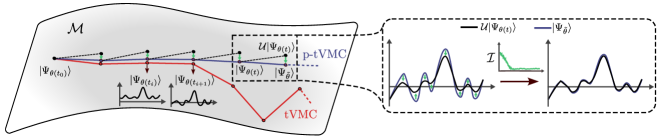
This condition may arise from the variational encoding of several physically relevant states, such as basis states , anti-symmetric wave functions (e.g. Slater, Neural Backflow [48], …) or states generated by digital quantum circuits. Another relevant class of affected states are those that underwent projective measurements, which are commonly found in trajectory unravelings of the Lindblad Master Equation [49, 50, 51] or in quantum information measurement protocols [4, 5, 6, 7, 8, 9, 10, 11, 12, 13, 14]. We remark that for continuous systems (such as a particle in free space), the bias may only emerge from zeros in the bulk, since at infinity the wave function and its derivative must vanish. A pictorial representation of the breakdown of tVMC is shown in Fig. 1.
In realistic calculations, the variational wave function is often arbitrarily close to zero without encoding nodes exactly. In such cases, the biases and are zero. Still, we find that the variances of and grow such that an exponential number of samples is required to resolve those quantities with finite accuracy. This phenomenon can be revealed by the signal-to-noise ratios (SNRs) of and approaching zero. The SNR of a function of random variable with distribution is:
| (10) |
In practical calculations, to ensure an accurate estimation with a finite number of samples we require . This inequality guarantees that the effective signal (mean value) is larger than the statistical fluctuations and thus it can be resolved.
In the following, we first discuss a minimal example where finite biases emerge, and we then consider a more realistic case where there are no biases but for which we show that the SNRs go to zero.
2.1 Paradigmatic examples
We analyze a toy model where the biases are non-zero, and they break the tVMC dynamics. The system is made by spin where the state is parameterized by the ansatz . For , such that , and evolution generated by Hamiltonian , we have that and in Eqs. 8 and 9 are finite and the stochastic estimates differ from the exact values as:
| (11) | ||||||
| (12) |
(see Section B.1 for the full calculation).
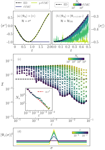
In Fig. 2(a) we show a simulation of an initial state which is rotated by the Hamiltonian . At the state becomes and the tVMC evolution is stuck, as and vanish. Similar considerations hold for more than 1 particle, and in Section B.2 we discuss an example for the GHZ state of spins.
We now analyze a more realistic case where the variational state does not exactly encode zeros. In particular, we consider a system of spins in the state , which is peaked on a single configuration and has a constant small amplitude for all the other basis states (see Fig. 2(d)), namely:
| (13) |
where . We remark that for small this ansatz approximates a Hartree-Fock state, which commonly arises from quantum-chemistry Hamiltonians. For the biases are zero, but for the leading terms of the SNRs for and are respectively (see Appendix C for the full calculation):
| (14) |
Intuitively, this suggests that the more peaked the state is, the more samples will be needed to accurately estimate those quantities, in particular . As normalization of the state imposes , the number of samples necessary to correctly compute the quantum geometric tensor and the variational forces will diverge as , eliminating the advantage of stochastic sampling and rendering tVMC computationally ineffective.
We consolidate this argument with a numerical experiment involving a commonly adopted setup for quantum dynamics. We evolve with tVMC the state for according to the Transverse Field Ising (TFI) Hamiltonian,
| (15) |
where denotes nearest neighbors in a lattice with periodic boundary conditions. In Fig. 2(b) we show some evolutions obtained with an increasing number of Monte Carlo samples for a fixed , demonstrating that the dynamics is correctly reconstructed only at large values of . The scaling of with the system size is studied in Fig. 2(c), where we report the final infidelity111The infidelity between two arbitrary states and is defined as . of the state obtained with tVMC with respect to the exact solution for different and . We remark that the accuracy of the variational simulation improves when or are increased, as the statistical fluctuations in the estimated quantities are suppressed. The inset highlights a power-law relation between the necessary to reconstruct the dynamics accurately and , proving that .
2.2 Overview
In this first section, we have shown that the tVMC method can be either biased or require an exponential number of samples when the wave function is exactly or approximately zero. This highlights the necessity of an efficient alternative method to tVMC for variational time evolution.
We stress that while our considerations on stochastic estimators arose in the context of tVMC, they are also applicable to ground-state calculations using both plain gradient descent or stochastic reconfiguration [52], because they rely on the same stochastic estimators. However, we believe that in such calculations, the additional errors contributed by the biasing or small SNR are mitigated by the iterative optimization scheme, which may avoid the accumulation of errors that instead affects dynamics. We also remark that Monte Carlo variational methods for open quantum systems [53, 54, 55, 56] are also possibly affected by the same issues.
Going forward, in Appendix A we propose a modified estimator for the forces for which the bias and the SNR problems are absent, and therefore it can efficiently estimate the forces when the standard estimator fails (see Appendices B and C). From our knowledge, this alternative estimator has never been discussed in the literature, and preliminary investigations suggest that it already reduces the computational effort needed to reliably find the ground state of some frustrated or fermionic Hamiltonians.
Unfortunately, we could not find a similarly straightforward modification of the estimator for the quantum geometric tensor . For that reason, the following section presents a completely different scheme that avoids using the tensor.
3 Projected time-dependent Variational Monte Carlo
We consider the general problem of finding the parameters of a variational state such that it approximates the state , where are known and is an arbitrary transformation, in terms of a given distance. Considering the distance to be the infidelity , this can be expressed as the following optimization problem:
| (16) |
Other distance choices, such as the L2 metric, have also been discussed in the literature [36]. Eq. 16 is similar to Eq. 2, but it can treat arbitrary unitaries and therefore can be used to simulate non-infinitesimal gates in quantum circuits [32, 33] or to perform state preparation.
The solution of Eq. 16 can be found with iterative gradient-based optimizers such as Stochastic Gradient Descent [57], ADAM [58], Natural Gradient [59, 60, 44] or similar methods. Since this approach consists of projecting the exactly evolved state onto the manifold of the variational ansatz , we name it projected time-dependent Variational Monte Carlo (p-tVMC), and this is pictorially represented in Fig. 1.
The infidelity in Eq. 16 can be estimated through Monte Carlo sampling as . Many choices for the sampling distribution and the local estimator are possible, but assuming that is unitary we can sample
| (17) |
from the joint Born distribution of the two states . For non-unitary it is necessary to sample from instead of [32, 33].
We remark that estimating the infidelity using Eq. 17 is efficient if is -local [61], namely it acts non-trivially on at most degrees of freedom (spins, qubits, particles, …), where is polynomially large in the system size. When this is not the case, it can be factored in several sub-terms where each term is -local, and Eq. 16 must be solved for every sub-unitary . In particular, the unitary propagator of a general Hamiltonian can be decomposed with the Trotter-Suzuki decomposition [62, 63] or with other expansions that are unitary up to leading order, such as the Taylor series [35].
We now analyze the estimator according to the same approach used in the previous section. We find that, in the limit of , the SNR of the estimator scales as
| (18) |
This means that, as the optimization approaches the optimum of , the number of samples needed to resolve the infidelity increases as (see Appendix E for analytical calculation). This is systematically different from what happens when minimizing the energy, where the SNR remains constant when close to the solution, and a constant number of samples can be used to achieve arbitrarily high precision.
To recover this behaviour in the case of the infidelity optimization we propose a new estimator based upon the Control Variates (CV) technique [64]:
| (19) |
where . The quantity can be chosen such that the attains a minimal value. This optimal value of , say , depends on the parameters of the ansatz, so it changes during an infidelity optimization. However, it is possible to show (see Appendix E for analytical proof) that in the limit , is exactly . Therefore, we avoid the high cost of estimating at each iteration of an optimization, and directly use the asymptotically ideal estimator Eq. 19 with .
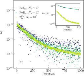
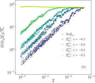
To further support this approach, we show in Fig. 3(a) that the CV estimator features a variance that is orders of magnitude smaller than the one of the bare estimator , in such a way that the number of samples needed for the optimization is reduced by almost three orders of magnitude. Additionally, the scaling of the variance with changes, such that for we have that:
| (20) |
meaning that the SNR remains asymptotically constant (see analytical proof in Appendix E). Indeed, in Fig. 3(b) one can see that the SNR of goes to zero when decreases, while the SNR of the corrected estimator decreases at smaller values of . When , has a rescaled SNR which is constant and larger than over the whole range of considered, suggesting that our strategy is ideal.
Moreover, the reduced variance of the CV estimator implies that the infidelity gradient computed with it results to be more accurate [65]. The lower-variance gradient can improve the accuracy of the solution, since its mean value is affected by smaller statistical fluctuations, and can increase the speed of convergence, as it allows for larger learning rates.
This substantial improvement of the sampling cost using the CV estimator Eq. 19 makes the p-tVMC an efficiently scalable method for simulating large systems, such that it can address system sizes that have not been investigated before within this approach. A detailed analysis on the CV infidelity estimator is present in Appendix E, with further extensions in Appendix F. As shown in Fig. 2(a), in Section B.2 for the GHZ state and in Appendix D for adiabatic evolution, the p-tVMC, since it is not affected by biases or vanishing SNR, can simulate dynamics in cases where tVMC fails or is inefficient.
4 Unitary dynamics with random measurements
In recent years, considerable interest has been devoted to studying entanglement in many-body quantum systems subject to evolution and random local measurements. This is a paradigmatic model of a quantum system coupled to an external environment acting as a measurement apparatus. Therefore, it is intimately related to the physics of open quantum systems. The competition between the unitary evolution’s entangling action and the measurements’ localizing effect gives rise to a phase transition between volume-law and area-law entanglement in the steady state of the dynamics. The order parameter is the measurement rate. This phenomenology has been originally investigated in quantum circuits [4, 5, 7, 9, 10, 11, 13, 14], and more recently for continuous dynamics [6, 8, 12].
To the extent of our knowledge, numerical investigations have focused so far on systems in one-dimension, integrable or evolving via efficiently simulable [66] Clifford gates because of algorithmic limitations. However, several open questions remain on the nature of such transitions in non-integrable 2D systems or non-Clifford circuits, requiring novel computational paradigms.
In this concluding section, we leverage the p-tVMC to simulate the time evolution generated by the (non-Clifford) 2D TFI model subject to random local measurements. This problem cannot be treated efficiently with Tensor Network methods because of the rapid entanglement growth and the exponential cost of exact contractions in 2D. Moreover, as projective measurements insert exponentially many zeros in the wave function amplitudes, the shortcomings of tVMC discussed in this article emerge, resulting in an exponential cost. We consider a 2D spin square lattice with side length , such that the total number of spins is . We evolve the system to time , discretized into time-steps of duration . At each , two operations are performed on the system:
-
•
unitary evolution with , where is the 2D TFI Hamiltonian of Eq. 15;
-
•
a projective measurement of each spin in the basis independently with probability (measurement rate).
The overall evolution is stochastic and non-unitary.
As the unitary propagator is not -local, we decompose it with a second-order Trotter scheme as:
| (21) |
where and .
In the first stages of this work we employed the forward-backward scheme as done in [36, 67], but then we move to the Trotterization as it allowed to use larger and was more practical for our calculations.
We use the p-tVMC to apply each unitary obtained from the decomposition. Still, we remark that as is diagonal in the chosen basis, its p-tVMC optimization problem can be solved analytically, as shown in Appendix G. Instead, the unitary containing is applied using the p-tVMC, factorizing the propagator into a product of terms, each of which acts on a small subset of the spins. In this way, the number of connected elements to compute is not exponentially large with . The unitary dynamics that we simulate is a global quench across the critical point of the 2D , which is in correspondence of the transverse field such that [68, 69, 70, 71, 72]. In particular, the initial state is the paramagnetic ground state in the limit , given by , and this is evolved into the ferromagnetic phase where .
The measurement operators are for . When a spin is measured, one of the two projectors is applied to the state according to the probabilities . Measurements can be exactly realized on a variational state by modifying it into a new ansatz with additional parameters defined as:
| (22) |
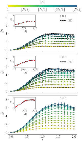
Measuring spin with outcome translates into setting and and vice versa for the other outcome. The measurement probabilities are stochastically computed using Monte Carlo sampling. The protocol of unitary evolution and random measurements is repeated several times and the final result is obtained by averaging over all these trajectories, as in the Monte Carlo wave function method [49]. To study the entanglement growth of , we monitor the Rényi-2 entanglement entropy , where is the reduced density matrix of the state on a subsystem . Indeed, the Rényi-2 entropy is a lower bound for the Von Neumann entanglement entropy and it can be estimated via Monte Carlo sampling [73] as:
| (23) |
where and (complementary of ). See Appendix H for a derivation of Eq. 23.
Fig. 4 shows the evolution of for subsystems of size in lattices with and with measurement rate . To assess the quality of the variational simulations, we compare with ED for and we select a feature density for the RBM ansatz employed (which determines its expressivity) that gives a satisfying level of precision. Given the chosen hyper-parameters, there is an excellent agreement for small subsystem sizes () and a good agreement for the largest partitions. The Rényi-2 entanglement entropy is 0 at , as expected for the initial product state, and it grows linearly over time, plateauing to a value that is proportional to . The Page-like curves [74] in the insets of Fig. 4 suggest that with the steady-states belong to a high-entanglement phase. However, due to possible finite size effects, whether the scaling of with the subsystem size is linear, witnessing a volume-law, or logarithmic as in critical phases is not obvious. In any case, a low-entanglement regime with area-law scaling is excluded since, in that situation, the steady-state would not change for subsystems with the same boundary length (indicated with equal markers in the insets). Instead, what is observed is that increases with independently of the boundary length, at least far from where finite size effects might play a role. The proportionality of the entanglement growth rate in the initial times with the boundaries of the partitions is in accordance with the Lieb-Robinson bound [75] valid for local Hamiltonians.
5 Conclusions
In this manuscript, we proved that the standard approach to Monte Carlo variational dynamics, the tVMC, can be limited by a finite bias or by an exponentially small signal-to-noise ratio when the wave function contains nodes or is only approximately zero. This implies that the tVMC cannot efficiently simulate the time evolution of physically-relevant cases such as completely polarized wave functions, states arising from digital quantum circuits or measurement processes, including the open dynamics with quantum jumps. Subsequently, we have formalized an alternative scheme, which consists in solving an optimization problem at each time step using the infidelity distance, and we have introduced a novel stochastic estimator which makes this approach viable and scalable to large systems. Finally, we showed that our method can solve the lack of efficient algorithms to investigate the high-entanglement phase in a protocol of non-Clifford unitary dynamics with local random measurements in 2D. This enables future investigation into the physics of several classes of systems, including measurement-induced phase transitions in non-trivial models above 1D and the physics of dissipative systems, all of which are currently limited by the available computational methods. In particular, a direct application of the projected method would be the variational simulation of quantum trajectories arising from unraveling the Lindblad Master Equation.
6 Data availability
7 Acknowledgments
F.V. warmly thanks A. Biella for inspirational, insightful discussions and V. Savona for arguments motivating this study. We gratefully acknowledge J. Nys and Z. Denis for fruitful comments and discussions. A.S. is supported by SEFRI under Grant No. MB22.00051 (NEQS - Neural Quantum Simulation). C.G. is supported by the Swiss National Science Foundation under Grant No. 200021_200336.
References
- [1] I. M. Georgescu, S. Ashhab, and F. Nori. “Quantum simulation”. Rev. Mod. Phys. 86, 153–185 (2014). doi: 10.1103/RevModPhys.86.153.
- [2] F. Minganti, I. I. Arkhipov, A. Miranowicz, and F. Nori. “Continuous dissipative phase transitions with or without symmetry breaking”. New Journal of Physics 23, 122001 (2021). doi: 10.1088/1367-2630/ac3db8.
- [3] M. A. Nielsen and I. L. Chuang. “Quantum computation and quantum information: 10th anniversary edition”. Cambridge University Press. (2010). doi: 10.1017/CBO9780511976667.
- [4] B. Skinner, J. Ruhman, and A. Nahum. “Measurement-induced phase transitions in the dynamics of entanglement”. Phys. Rev. X 9, 031009 (2019). doi: 10.1103/PhysRevX.9.031009.
- [5] Y. Li, X. Chen, and M. P. A. Fisher. “Measurement-driven entanglement transition in hybrid quantum circuits”. Phys. Rev. B 100, 134306 (2019). doi: 10.1103/PhysRevB.100.134306.
- [6] Q. Tang and W. Zhu. “Measurement-induced phase transition: A case study in the nonintegrable model by density-matrix renormalization group calculations”. Phys. Rev. Res. 2, 013022 (2020). doi: 10.1103/PhysRevResearch.2.013022.
- [7] X. Turkeshi, R. Fazio, and M. Dalmonte. “Measurement-induced criticality in -dimensional hybrid quantum circuits”. Phys. Rev. B 102, 014315 (2020). doi: 10.1103/PhysRevB.102.014315.
- [8] X. Turkeshi, A. Biella, R. Fazio, M. Dalmonte, and M. Schiró. “Measurement-induced entanglement transitions in the quantum ising chain: From infinite to zero clicks”. Phys. Rev. B 103, 224210 (2021). doi: 10.1103/PhysRevB.103.224210.
- [9] A. Lavasani, Y. Alavirad, and M. Barkeshli. “Topological order and criticality in monitored random quantum circuits”. Phys. Rev. Lett. 127, 235701 (2021). doi: 10.1103/PhysRevLett.127.235701.
- [10] O. Lunt, M. Szyniszewski, and A. Pal. “Measurement-induced criticality and entanglement clusters: A study of one-dimensional and two-dimensional clifford circuits”. Phys. Rev. B 104, 155111 (2021). doi: 10.1103/PhysRevB.104.155111.
- [11] H. Liu, T. Zhou, and X. Chen. “Measurement-induced entanglement transition in a two-dimensional shallow circuit”. Phys. Rev. B 106, 144311 (2022). doi: 10.1103/PhysRevB.106.144311.
- [12] X. Turkeshi, M. Dalmonte, R. Fazio, and M. Schiró. “Entanglement transitions from stochastic resetting of non-hermitian quasiparticles”. Phys. Rev. B 105, L241114 (2022). doi: 10.1103/PhysRevB.105.L241114.
- [13] P. Sierant, M. Schiró, M. Lewenstein, and X. Turkeshi. “Measurement-induced phase transitions in -dimensional stabilizer circuits”. Phys. Rev. B 106, 214316 (2022). doi: 10.1103/PhysRevB.106.214316.
- [14] J. C. Hoke et al. “Quantum information phases in space-time: measurement-induced entanglement and teleportation on a noisy quantum processor” (2023). arXiv:2303.04792.
- [15] S. R. White. “Density matrix formulation for quantum renormalization groups”. Phys. Rev. Lett. 69, 2863–2866 (1992). doi: 10.1103/PhysRevLett.69.2863.
- [16] R. Orús. “A practical introduction to tensor networks: Matrix product states and projected entangled pair states”. Annals of physics 349, 117–158 (2014). doi: 10.1016/j.aop.2014.06.013.
- [17] D. Ceperley and B. Alder. “Quantum monte carlo”. Science 231, 555–560 (1986). doi: 10.1126/science.231.4738.555.
- [18] W. M. C. Foulkes, L. Mitas, R. J. Needs, and G. Rajagopal. “Quantum monte carlo simulations of solids”. Rev. Mod. Phys. 73, 33–83 (2001). doi: 10.1103/RevModPhys.73.33.
- [19] M. Troyer and U.-J. Wiese. “Computational complexity and fundamental limitations to fermionic quantum monte carlo simulations”. Phys. Rev. Lett. 94, 170201 (2005). doi: 10.1103/PhysRevLett.94.170201.
- [20] K. Choo, A. Mezzacapo, and G. Carleo. “Fermionic neural-network states for ab-initio electronic structure”. Nature Communications11 (2020). doi: 10.1038/s41467-020-15724-9.
- [21] D. Pfau, J. S. Spencer, A. G. D. G. Matthews, and W. M. C. Foulkes. “Ab initio solution of the many-electron schrödinger equation with deep neural networks”. Phys. Rev. Research 2, 033429 (2020). doi: 10.1103/PhysRevResearch.2.033429.
- [22] Y. Nomura, A. S. Darmawan, Y. Yamaji, and M. Imada. “Restricted boltzmann machine learning for solving strongly correlated quantum systems”. Phys. Rev. B 96, 205152 (2017). doi: 10.1103/PhysRevB.96.205152.
- [23] J. Stokes, J. R. Moreno, E. A. Pnevmatikakis, and G. Carleo. “Phases of two-dimensional spinless lattice fermions with first-quantized deep neural-network quantum states”. Phys. Rev. B 102, 205122 (2020). doi: 10.1103/PhysRevB.102.205122.
- [24] J. Nys and G. Carleo. “Variational solutions to fermion-to-qubit mappings in two spatial dimensions”. Quantum 6, 833 (2022). doi: 10.22331/q-2022-10-13-833.
- [25] K. Choo, T. Neupert, and G. Carleo. “Two-dimensional frustrated model studied with neural network quantum states”. Phys. Rev. B 100, 125124 (2019). doi: 10.1103/PhysRevB.100.125124.
- [26] O. Sharir, Y. Levine, N. Wies, G. Carleo, and A. Shashua. “Deep autoregressive models for the efficient variational simulation of many-body quantum systems”. Phys. Rev. Lett. 124, 020503 (2020). doi: 10.1103/PhysRevLett.124.020503.
- [27] D. Wu et al. “Variational benchmarks for quantum many-body problems” (2023) arXiv:2302.04919.
- [28] W. L. McMillan. “Ground state of liquid ”. Phys. Rev. 138, A442–A451 (1965). doi: 10.1103/PhysRev.138.A442.
- [29] X. Yuan, S. Endo, Q. Zhao, Y. Li, and S. C. Benjamin. “Theory of variational quantum simulation”. Quantum 3, 191 (2019). doi: 10.22331/q-2019-10-07-191.
- [30] G. Carleo, F. Becca, M. Schiró, and M. Fabrizio. “Localization and glassy dynamics of many-body quantum systems”. Scientific Reports2 (2012). doi: 10.1038/srep00243.
- [31] G. Carleo, L. Cevolani, L. Sanchez-Palencia, and M. Holzmann. “Unitary dynamics of strongly interacting bose gases with the time-dependent variational monte carlo method in continuous space”. Phys. Rev. X 7, 031026 (2017). doi: 10.1103/PhysRevX.7.031026.
- [32] B. Jónsson, B. Bauer, and G. Carleo. “Neural-network states for the classical simulation of quantum computing” (2018). arXiv:1808.05232.
- [33] M. Medvidović and G. Carleo. “Classical variational simulation of the quantum approximate optimization algorithm”. npj Quantum Information 7, 1–7 (2021). doi: 10.1038/s41534-021-00440-z.
- [34] S. Barison, F. Vicentini, and G. Carleo. “An efficient quantum algorithm for the time evolution of parameterized circuits”. Quantum 5, 512 (2021). doi: 10.22331/q-2021-07-28-512.
- [35] K. Donatella, Z. Denis, A. Le Boité, and C. Ciuti. “Dynamics with autoregressive neural quantum states: Application to critical quench dynamics”. Phys. Rev. A 108, 022210 (2023). doi: 10.1103/PhysRevA.108.022210.
- [36] I. L. Gutiérrez and C. B. Mendl. “Real time evolution with neural-network quantum states”. Quantum 6, 627 (2022). doi: 10.22331/q-2022-01-20-627.
- [37] M. Schmitt and M. Heyl. “Quantum many-body dynamics in two dimensions with artificial neural networks”. Phys. Rev. Lett. 125, 100503 (2020). doi: 10.1103/PhysRevLett.125.100503.
- [38] R. Verdel, M. Schmitt, Y.-P. Huang, P. Karpov, and M. Heyl. “Variational classical networks for dynamics in interacting quantum matter”. Phys. Rev. B 103, 165103 (2021). doi: 10.1103/PhysRevB.103.165103.
- [39] M. Schmitt, M. M. Rams, J. Dziarmaga, M. Heyl, and W. H. Zurek. “Quantum phase transition dynamics in the two-dimensional transverse-field ising model”. Science Advances 8, eabl6850 (2022). doi: 10.1126/sciadv.abl6850.
- [40] M. V. den Nest. “Simulating quantum computers with probabilistic methods” (2010). arXiv:0911.1624.
- [41] N. Moiseyev. “Non-hermitian quantum mechanics”. Cambridge University Press. (2011). doi: 10.1017/CBO9780511976186.
- [42] S. Haroche and J.-M. Raimond. “Exploring the Quantum: Atoms, Cavities, and Photons”. Oxford University Press. (2006). doi: 10.1093/acprof:oso/9780198509141.001.0001.
- [43] A. McLachlan. “A variational solution of the time-dependent schrodinger equation”. Molecular Physics 8, 39–44 (1964). doi: 10.1080/00268976400100041.
- [44] J. Stokes, J. Izaac, N. Killoran, and G. Carleo. “Quantum Natural Gradient”. Quantum 4, 269 (2020). doi: 10.22331/q-2020-05-25-269.
- [45] C.-Y. Park and M. J. Kastoryano. “Geometry of learning neural quantum states”. Phys. Rev. Res. 2, 023232 (2020). doi: 10.1103/PhysRevResearch.2.023232.
- [46] L. Hackl, T. Guaita, T. Shi, J. Haegeman, E. Demler, and J. I. Cirac. “Geometry of variational methods: dynamics of closed quantum systems”. SciPost Phys. 9, 048 (2020). doi: 10.21468/SciPostPhys.9.4.048.
- [47] G. Carleo and M. Troyer. “Solving the quantum many-body problem with artificial neural networks”. Science 355, 602–606 (2017). doi: 10.1126/science.aag2302.
- [48] D. Luo and B. K. Clark. “Backflow transformations via neural networks for quantum many-body wave functions”. Phys. Rev. Lett. 122, 226401 (2019). doi: 10.1103/PhysRevLett.122.226401.
- [49] K. Mølmer, Y. Castin, and J. Dalibard. “Monte carlo wave-function method in quantum optics”. J. Opt. Soc. Am. B 10, 524–538 (1993). doi: 10.1364/JOSAB.10.000524.
- [50] H. M. Wiseman and G. J. Milburn. “Quantum measurement and control”. Cambridge University Press. (2009). doi: 10.1017/CBO9780511813948.
- [51] F. Minganti, D. Huybrechts, C. Elouard, F. Nori, and I. I. Arkhipov. “Creating and controlling exceptional points of non-hermitian hamiltonians via homodyne lindbladian invariance”. Phys. Rev. A 106, 042210 (2022). doi: 10.1103/PhysRevA.106.042210.
- [52] S. Sorella, M. Casula, and D. Rocca. “Weak binding between two aromatic rings: Feeling the van der Waals attraction by quantum Monte Carlo methods”. The Journal of Chemical Physics127 (2007). doi: 10.1063/1.2746035.
- [53] F. Vicentini, A. Biella, N. Regnault, and C. Ciuti. “Variational neural-network ansatz for steady states in open quantum systems”. Phys. Rev. Lett. 122, 250503 (2019). doi: 10.1103/PhysRevLett.122.250503.
- [54] M. J. Hartmann and G. Carleo. “Neural-network approach to dissipative quantum many-body dynamics”. Phys. Rev. Lett. 122, 250502 (2019). doi: 10.1103/PhysRevLett.122.250502.
- [55] A. Nagy and V. Savona. “Variational quantum monte carlo method with a neural-network ansatz for open quantum systems”. Phys. Rev. Lett. 122, 250501 (2019). doi: 10.1103/PhysRevLett.122.250501.
- [56] M. Reh, M. Schmitt, and M. Gärttner. “Time-dependent variational principle for open quantum systems with artificial neural networks”. Phys. Rev. Lett. 127, 230501 (2021). doi: 10.1103/PhysRevLett.127.230501.
- [57] I. Sutskever, J. Martens, G. Dahl, and G. Hinton. “On the importance of initialization and momentum in deep learning”. In S. Dasgupta and D. McAllester, editors, Proceedings of the 30th International Conference on Machine Learning. Volume 28 of Proceedings of Machine Learning Research, pages 1139–1147. Atlanta, Georgia, USA (2013). PMLR. url: https://proceedings.mlr.press/v28/sutskever13.html.
- [58] D. P. Kingma and J. Ba. “Adam: A method for stochastic optimization” (2017). arXiv:1412.6980.
- [59] S.-i. Amari. “Natural Gradient Works Efficiently in Learning”. Neural Computation 10, 251–276 (1998). doi: 10.1162/089976698300017746.
- [60] S. Sorella. “Wave function optimization in the variational monte carlo method”. Phys. Rev. B 71, 241103 (2005). doi: 10.1103/PhysRevB.71.241103.
- [61] J. Yan and D. Bacon. “The k-local pauli commuting hamiltonians problem is in p” (2012). arXiv:1203.3906.
- [62] H. F. Trotter. “On the product of semi-groups of operators”. In Proceedings of the American Mathematical Society. Volume 151, pages 545–551. (1959). doi: 10.1090/S0002-9939-1959-0108732-6.
- [63] M. Suzuki. “General theory of fractal path integrals with applications to many‐body theories and statistical physics”. Journal of Mathematical Physics 32, 400–407 (1991). doi: 10.1063/1.529425.
- [64] R. Y. Rubinstein and D. P. Kroese. “Simulation and the monte carlo method”. John Wiley & Sons. (2016). doi: 10.1002/9781118631980.
- [65] S. Mohamed, M. Rosca, M. Figurnov, and A. Mnih. “Monte carlo gradient estimation in machine learning”. The Journal of Machine Learning Research 21, 5183–5244 (2020). url: http://jmlr.org/papers/v21/19-346.html.
- [66] D. Gottesman. “The heisenberg representation of quantum computers” (1998). arXiv:quant-ph/9807006.
- [67] D. Luo, Z. Chen, K. Hu, Z. Zhao, V. M. Hur, and B. K. Clark. “Gauge-invariant and anyonic-symmetric autoregressive neural network for quantum lattice models”. Phys. Rev. Res. 5, 013216 (2023). doi: 10.1103/PhysRevResearch.5.013216.
- [68] R. J. Elliott, P. Pfeuty, and C. Wood. “Ising model with a transverse field”. Phys. Rev. Lett. 25, 443–446 (1970). doi: 10.1103/PhysRevLett.25.443.
- [69] M. S. L. du Croo de Jongh and J. M. J. van Leeuwen. “Critical behavior of the two-dimensional ising model in a transverse field: A density-matrix renormalization calculation”. Phys. Rev. B 57, 8494–8500 (1998). doi: 10.1103/PhysRevB.57.8494.
- [70] H. Rieger and N. Kawashima. “Application of a continuous time cluster algorithm to the two-dimensional random quantum ising ferromagnet”. The European Physical Journal B - Condensed Matter and Complex Systems 9, 233–236 (1999). doi: 10.1007/s100510050761.
- [71] H. W. J. Blöte and Y. Deng. “Cluster monte carlo simulation of the transverse ising model”. Phys. Rev. E 66, 066110 (2002). doi: 10.1103/PhysRevE.66.066110.
- [72] A. F. Albuquerque, F. Alet, C. Sire, and S. Capponi. “Quantum critical scaling of fidelity susceptibility”. Phys. Rev. B 81, 064418 (2010). doi: 10.1103/PhysRevB.81.064418.
- [73] M. B. Hastings, I. González, A. B. Kallin, and R. G. Melko. “Measuring renyi entanglement entropy in quantum monte carlo simulations”. Phys. Rev. Lett. 104, 157201 (2010). doi: 10.1103/PhysRevLett.104.157201.
- [74] D. N. Page. “Average entropy of a subsystem”. Phys. Rev. Lett. 71, 1291–1294 (1993). doi: 10.1103/PhysRevLett.71.1291.
- [75] S. Bravyi, M. B. Hastings, and F. Verstraete. “Lieb-robinson bounds and the generation of correlations and topological quantum order”. Physical review letters 97, 050401 (2006). doi: 10.1103/PhysRevLett.97.050401.
- [76] F. Vicentini et al. “NetKet 3: Machine Learning Toolbox for Many-Body Quantum Systems”. SciPost Phys. CodebasesPage 7 (2022). doi: 10.21468/SciPostPhysCodeb.7.
- [77] G. Carleo et al. “NetKet: A machine learning toolkit for many-body quantum systems”. SoftwareXPage 100311 (2019). doi: 10.1016/j.softx.2019.100311.
- [78] D. Häfner and F. Vicentini. “mpi4jax: Zero-copy MPI communication of JAX arrays”. Journal of Open Source Software6 (2021). doi: 10.21105/joss.03419.
- [79] A. Sinibaldi and F. Vicentini. “netket_fidelity package, v0.0.2”. doi: 10.5281/zenodo.8344170.
- [80] V. Havlicek. “Amplitude Ratios and Neural Network Quantum States”. Quantum 7, 938 (2023). doi: 10.22331/q-2023-03-02-938.
Appendix
Appendix A Unbiased force estimate
An unbiased estimate for the variational forces can be obtained by inserting the completeness relation between and , instead of between and as done for the standard tVMC estimate , yielding:
| (24) | ||||
where, like in the main text, is the local energy and are the log-derivatives of the ansatz. does not have a covariance form like , therefore it has, in general, larger statistical fluctuations when estimated using a finite number of samples. Moreover, since cannot be used to compute the first term in Eq. 24, its computational cost is generally higher than the standard estimator.
Appendix B Examples of biases in tVMC
B.1 One-spin system
We consider a system of spin whose state is represented by the variational ansatz with parameters . The evolution is generated by the Hamiltonian . For the choice and , we have , and . In these conditions:
| (25) |
However, due to the covariance form of the standard tVMC estimates and evaluated on samples including only one value of , we have that :
| (26) |
We verify that, instead, the stochastic estimate with the alternative estimator proposed in the previous section is unbiased, since:
| (27) |
as .
B.2 Two-spin system
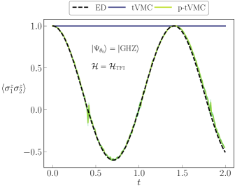
We consider a system of spins whose state is represented by the variational ansatz with parameters . For the ansatz represents the Greenberger–Horne–Zeilinger state . The variational derivatives are , , and . We consider the dynamics generated by the TFI Hamiltonian with coupling and transverse field . In these conditions, and differ from and as:
| (28) |
One can verify that, like for the one spin case, the alternative estimator gives an unbiased estimate for the variational forces. As shown in Eq. 28, has a lower rank than , while is identical to zero meaning that this dynamics starting from cannot be evolved with tVMC. On the contrary, the p-tVMC is not affected by any problem and can perform the evolution, as shown in Fig. 5.
Appendix C Signal to noise ratios in Monte Carlo estimates
We consider a system of spins and normalized variational states whose wave function is parameterized by a single parameter as:
| (29) |
with and for a given . In the following, we prove that the signal-to-noise ratios (SNRs) of and scale as , namely they diminish indefinitely as the wave function becomes more peaked around . In order to ensure normalization of over different system sizes, goes as . Therefore, the two SNRs diminish exponentially as increases, and so the number of samples needed to resolve and with finite precision is exponentially large in the system size. Instead, the SNR of the unbiased estimate of Eq. 24 is in , enabling it to efficiently estimate the forces in the limit , where cannot be used, and independently of the system size.
Proof.
The variational log-derivative of is:
| (30) |
We define for brevity and we observe that when . Both and are of the form , where and for some functions and of random variable with distribution . In we have and , while in we have and . The variance of stochastic estimates of this form is given by:
| (31) |
For the local energy we have:
| (32) | ||||
| (33) |
where the notation for any is used. Therefore, keeping leading order terms in , the variances of the stochastic estimates are:
| (34) |
Since and for , we have that:
| (35) |
The two SNRs go to zero when the state becomes more peaked because when we have that for , so these configurations are rarely sampled, but the estimators of the biases for increase as is reduced. Indeed, for we have that:
| (36) |
It is possible to verify that using the unbiased force estimate of Eq. 24 the SNR remains constant in the limit , making it able to efficiently compute the variational forces when the standard estimate fails. This is because the original sum of the first term in Eq. 24 already runs over the points where the wave function is non-zero, so to obtain the corresponding estimator it is sufficient to divide by without excluding any point. Instead, to obtain the estimator of the first term in the expression of it is necessary to divide by , implicitly excluding from the Monte Carlo expression the points for which the bias can be non-zero. Considering only the contribution of the first term in , since this is the problematic one in the standard estimate and the second term is common to , we obtain that:
| (37) |
Therefore, since for , we have:
| (38) |
∎
Appendix D Example of vanishing SNRs in tVMC
We consider a chain of spins , initially in the ground state of the Hamiltonian , which evolves according to the time-dependent Hamiltonian:
| (39) |
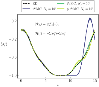
where oscillates between and with a triangular profile of period , namely if and if . It is known that for a sufficiently large , so for an adiabatic evolution, the state at is going to be -close to , so an instance of the peaked states of the previous section for some depending on .
While in this case the biases in the tVMC estimates are zero, in Fig. 6 we show that the dynamics is correctly reconstructed for only when choosing a sufficiently large number of samples (the Hilbert space in this case has size ), hinting at the exponentially small SNRs of and . As before, the p-tVMC can efficiently simulate this dynamics with a fair number of samples, for which instead the tVMC fails.
Appendix E Infidelity estimator with control variates
The stochastic estimate of the infidelity between the states and , where and are variational states and is an arbitrary transformation, is obtained by inserting completeness relations and dividing by wave function amplitudes in its definition as follows:
| (40) |
where is the term in brackets and .
Similarly, the (conjugate) gradient of the infidelity can be computed stochastically as:
| (41) |
where . We remark that the first term in the previous expression is free from the problem present in and when . Indeed, in this limit we have that for where the term vanishes, so the bias as in Eq. 8 disappears. Since we consider continuous time dynamics generated by a succession of infinitesimal s, such that already at the beginning of the optimizations, we can use the gradient Eq. 41 without incurring in the issues discussed for the tVMC.
The variance of can be directly computed from the one of as:
| (42) |
This proves that has a variance bounded above by (because ), as already noted in Ref. [80] of the main text, and that it features a zero variance principle, since when the solution is approached (), as the energy in VMC for ground state search. However, the SNR of is:
| (43) |
which vanishes when . This entails that when approaching the solution the number of samples must diverge as to resolve the infidelity with finite accuracy.
We find that this problem of diverging sampling overhead can be eliminated by applying the Control Variates (CV) technique on . Since is real, can be considered in place of in all the following. CV consists of adding to an estimator an additional random variable that is correlated to the estimator and for which the expectation value is known exactly, such that the fluctuations of this variable cancel out the ones of the original estimator. For the infidelity, we discovered that satisfies the required properties, since it is correlated to and we have . Therefore, we can define the CV infidelity estimator:
| (44) |
where . has the same mean as for any , while its variance depends on . Therefore, can be chosen such that is minimized. This optimal value, say , is:
| (45) |
where is the covariance of functions and of random variable with distribution . The corresponding minimized variance is:
| (46) |
which is smaller than . from Eq. 45 depends on the parameters of the variational ansatz, thus its value varies during the optimization. However, it is possible to prove that when , tends to , such that we can fix when is smaller than a predetermined value and avoid to re-estimate at each iteration. The limit value of can be proven analytically considering that when we have and with same order as . Therefore, computing reduces to solve .
For reasons similar to the ones previously discussed for the first term in Eq. 41, the estimation of the CV factor is not affected by a bias or a vanishing SNR as and when , and it is precisely in this limit where CV acts to keep the SNR constant. Therefore, is a well-defined infidelity estimator.
Appendix F Infidelity estimator with importance sampling
The estimator is unbounded because it contains ratios of wave function amplitudes. Therefore, it may diverge if and or and differ of orders of magnitudes. This is a severe problem when evolving the variational state after local measurements, since it may happen that on some configurations the state is close to zero but is not. Therefore, despite these configurations are rarely sampled, the estimator on them can be very large, significantly skewing the statistics. A way to include these outliers in the sampling is to perform importance sampling (see Ref. [64] of the main text), namely by rewriting:
| (47) |
for a given distribution . This latter can be chosen such that it minimizes the variance of the estimator, leading to the expression:
| (48) |
where . Using in place of , importance sampling can be combined with control variates obtaining the estimator:
| (49) |
The cost of importance sampling is almost times larger than the cost of standard sampling, where is the number of spins on which acts non-trivially.
Appendix G Exact application of a diagonal propagator
The exact solution of the general optimization problem in the p-tVMC must satisfy:
| (50) |
for all configurations and any constant equal for all . For certain and variational states, Eq. 50 can be solved exactly. In particular, if is diagonal in the basis and if it is possible to write with some update , Eq. 50 is reduced to:
| (51) |
where is the eigenvalue of for the eigenstate . In the following, we consider spin systems for simplicity. For the RBM, Eq. 51 admits a solution when consisting in an update of the visible bias only. If , instead, a simple parameter update is not sufficient. The transformation can be exactly implemented by adding a hidden unit (see Refs. [32, 33] of the main text). However, in general, starting with an arbitrary ansatz , it is possible to add two variational terms such that both and can be exactly simulated with a parameter change. Indeed, can be modified into a new ansatz with two additional parameters which is defined as:
| (52) |
The two exponential terms factorize as required to have Eq. 51, such that the application of translates into the updates , and , while for the changes , and are required. Adding many two-site terms in the ansatz, it is possible to simulate the dynamics of the diagonal part of the TFI Hamiltonian exactly.
Appendix H Stochastic estimator for the Rényi-2 entropy
An estimator for the Rényi-2 entanglement entropy can be obtained by explicitly writing the definition of the purity of the reduced density matrix:
| (53) |
where indicates the partial trace over , and . Now, inserting a further completeness relation in and dividing by wave function amplitudes one obtains:
| (54) |
