Effects of exact kinematics and the Sudakov
form factor on the dipole amplitude

Abstract

We investigate effects of exact gluon kinematics on the parameters of the Golec-Biernat–Wüsthoff, and Bartels–Golec-Biernat–Kowalski saturation models. The resulting fits show some differences, particularly, in the normalization of the dipole cross section $\sigma_{0}$. The refitted models are used for the dijet production process in DIS to investigate effects of the Sudakov form factor at Electron Ion Collider energies.

IFJPAN-IV-2023-2

1 Introduction

Figure 1: Kinematic variables of the inclusive DIS.

Factorization of scales plays central role in Quantum Chromodynamics (QCD). In particular, within collinear factorization approach, long-distance effects can be isolated into objects called collinear parton distribution functions (PDFs) [1, 2]. The collinear PDFs are not fully perturbatively calculable but they obey perturbative evolution equations and are process-independent [2]. That is to say that one needs to determine initial condition by fit to data, and the obtained PDFs can be used universally.

One of the main type of processes that is suited particularly well to the studies of proton structure is the deep inelastic scattering (DIS) [1, 2]. The data from HERA has enabled us to answer many questions in that domain and largely improved our picture of interior of a proton. It is therefore very exiting that the next generation of DIS machines, the Election Ion Collider (EIC) [3] is making its way and will soon allow us to uncover more details about hadron structure.

At large center of mass energy and fixed value of the photon virtuality, $Q$, one probes the region of small Bjorken scaling variable, $x$. In that region, which is dominated by gluons [1, 2, 4], the approach of High Energy Factorization, also called $k_{T}$-factorization [5, 6, 7, 8, 9, 10], has proven to be suited particularly well. In this framework, the interaction of the photon with gluons happens through boson-gluon fusion or quark impact factor, as depicted in Fig. 1. An object, which is central to the description of such process is called the dipole gluon density, $\mathcal{F}^{\mathrm{dipole}}(x,k_{T}^{2})$, and it is a type of transverse momentum dependent (TMD) [11, 12, 13, 14] PDF. Due to its clear picture, one often uses a position-space counterpart of the gluon density, called dipole cross section. It appears in the $k_{T}$-factorization formula [6, 12, 13, 14], which we shall discuss in the next section, and plays a role similar to that of the collinear parton distribution function in the collinear factorization.

Much effort has been made to study this object, notably the work of Balitsky, Fadin, Kuraev and Lipatov (BFKL) [15, 16] has predicted sharp rise of cross sections with $1/x$. However, such rise violates unitarity and the Froissart bound [1, 2, 4, 17]. In Ref. [18] it has been recognized that gluon recombination can tame the growth of gluons. The interplay of linear and nonlinear terms leads to a phenomenon called gluon saturation and corresponding evolution equations are known as Balitsky-Kovchegov (BK) [19, 20] equation or JIMWLK[21, 22, 23, 24, 25, 26] equation.

Despite the success of the aforementioned evolution equations, there exist a number of phenomenological models of the dipole cross section, which are popular due to to their simplicity. A notable example is the model proposed by Golec-Biernat and Wus̈thoff (GBW) [27] and its extension by Bartels, Golec-Biernat and Kowalski (BGK) [28]. We will use these two specific models in our study. We note, however, that other saturation models have been discussed in the literature [29, 30, 31, 32].

In the present study, we fit the GBW and BGK models to HERA data [33] in the $k_{T}$-factorization formula for $F_{2}$, instead of the original dipole factorization [34] formula. As discussed below, this allows us to relatively easy investigate the role of the exact gluon kinematics. Since inclusive observables do not reveal the $k_{T}$ dependence well, in order to demonstrate the effects of exact kinematics we consider a less inclusive observable which is more sensitive to the $k_{T}$ dependence of the gluon distribution. The resulting models are used for predictions of dijet production in DIS at Electron Ion Collider (EIC) [35], including effects of the Sudakov form factor, which resums logarithms of the small transverse momentum. This process is known to be sensitive to another type of gluon density, called Weitzsäcker-Williams (WW) [12, 13]. For that process, we study, in particular, the angular correlation of jets, and that of the scattered electron and the jets. For other papers addressing dijet production at the EIC we refer the Reader to [36, 37, 38, 39, 40].

The paper is organized as follows. In the next section, we present theoretical framework which we use and outline differences between the $k_{T}$-factorization and the dipole factorization. In Sec. 3, results of the new fits to HERA data in the $k_{T}$-factorization formula are presented. In Sec. 4, we apply the results from the previous section to compute distributions for dijet production in DIS at the EIC and make comparisons to our earlier study of Ref. [41].

2 The framework

The DIS cross section (structure function) factorises and can be written in a form

$$d\sigma=\sum_{a}\phi_{a/h}\otimes H_{\gamma a\to X},$$ (1)

where the hard function, $H_{\gamma a\to X}$, involving a parton $a$ in the initial state, is calculable perturbatively, and $\phi_{a/h}$ is the parton distribution function of $a$ in a hadron $h$. The symbol $\otimes$ denotes appropriate convolution. All nonperturbative effects are absorbed in $\phi_{a/h}$, while $H_{\gamma a\to X}$ can be computed order by order in $\alpha_{s}$.

We will study factorization in two versions: defined in momentum and position space, respectively. As mentioned earlier, in the fit, we use the GBW and BGK models. The models were originally formulated in the position-space version of the $k_{T}$-factorization formula. In the GBW model, the dipole cross section has the form [27]

$$\sigma_{\mathrm{GBW}}(x,r) =\sigma_{0}\left(1-e^{-r^{2}/R^{2}_{0}}\right) \mathrm{where} R^{-2}_{0} =\frac{Q_{0}^{2}}{4}\left(\frac{x_{0}}{x}\right)^{\lambda}.$$ (2)

The dipole cross section is related to the dipole gluon density by the Fourier transform

$$\alpha_{s}\mathcal{F}^{\mathrm{dipole}}(x,k_{T}^{2})=\frac{N_{c}}{4\pi}\int\frac{d^{2}\mathbf{r}}{(2\pi)^{2}}e^{i\mathbf{k}_{t}\cdot\mathbf{r}}\nabla_{\mathbf{r}}^{2}\sigma_{\mathrm{dipole}}(x,r).$$ (3)

The essence of the GBW model is encoded in the $x$-dependent saturation scale $Q_{s}^{2}(x)=Q^{2}_{0}(x_{0}/x)^{-\lambda}$, which separates the saturation region and the scaling region. An extension of the above model was proposed by Bartels, Golec-Biernat and Kowalski [28] who incorporated the DGLAP evolution in the GBW dipole cross section (2) by modifying the exponent to

$$R_{0}^{-2}=\frac{\pi^{2}\alpha(\mu^{2})xg(x,\mu^{2})}{3\sigma_{0}},$$ (4)

where

$$\mu^{2} =\frac{C}{r^{2}}+\mu_{0}^{2} \mathrm{and} xg(x,Q^{2}_{0}) =A_{g}x^{-\lambda_{g}}(1-x)^{5.6},$$ (5)

thus improving the description of data at higher $Q^{2}$.

While these models enjoyed much success in the phenomenology of DIS, including the diffractive and photo-production processes [27, 42], it is worth mentioning that they both use certain kinematic approximation which is specific to LO dipole factorization and are not there in the $k_{T}$-factorization. This was recognized in [43]. In the following, we will investigate effects of these approximations.

Firstly, let us outline the factorization formulas. With $q^{\prime}\equiv q+xp$, one decomposes $k$ and $\kappa$, defined in Fig. 1, as

$$\kappa =\alpha p-\beta q^{\prime}+\kappa_{t} \mathrm{and} k =ap-bq^{\prime}+k_{T}.$$ (6)

For the contribution depicted in Fig. 1, the structure function $F_{2}$ factorizes with a change of variable ${\boldsymbol{\kappa}^{\prime}}_{t}\equiv{\boldsymbol{\kappa}_{t}}-(1-\beta)\mathbf{k}_{t}$, to the form [44, 45]

$$F_{2}(x,Q^{2})=\sum_{f}e_{f}^{2}\frac{Q^{2}}{2\pi}\int\frac{dk^{2}_{t}}{k_{T}^{2}}\int^{1}_{0}d\beta\int d{\kappa^{\prime}}_{t}\alpha_{s}(\mu^{2})\mathcal{F}^{\mathrm{dipole}}(x/z,k_{T}^{2})\Theta(1-x/z)\\ \left[\left(\beta^{2}+(1-\beta)^{2}\right)\left(\frac{I_{1}}{2\pi}-\frac{I_{2}}{2\pi}\right)+\left(m_{f}^{2}+4Q^{2}\beta^{2}(1-\beta)^{2}\right)\left(\frac{I_{3}}{2\pi}-\frac{I_{4}}{2\pi}\right)\right],$$ (7)

where

$$\frac{1}{z}=1+\frac{{\kappa^{\prime}}^{2}_{t}+m_{f}^{2}}{\beta(1-\beta)Q^{2}}+\frac{k^{2}_{t}}{Q^{2}}\,.$$ (8)

One should note that the gluons are not probed directly, thus the argument of the gluon density is $x/z$ rather than $x$. If one, instead, uses $1/z=1+4m_{f}^{2}/Q^{2}$ and assumes that $\mu$ is independent of $\kappa^{\prime}$ and $k_{T}$, the above formula can be written in the impact parameter space [27, 46] (i.e. as a dipole factorization formula)

$$F_{2}\left(x,Q^{2}\right)=\sum_{f}e_{f}^{2}\frac{Q^{2}}{4\pi^{2}}\int^{1}_{0}d\beta\int\frac{d^{2}\mathbf{r}}{(2\pi)^{2}}\left|\Psi\left(\tilde{x},\beta,Q^{2}\right)\right|^{2}\sigma_{\mathrm{dipole}}\left(\tilde{x},r\right),$$ (9)

where the photon wave function, $\left|\Psi\left(x,\beta,Q^{2}\right)\right|^{2}$, describes splitting of the incoming photon into a $q\overline{q}$ pair with light-cone momenta fractions $\beta$ and $1-\beta$ respectively, and the dipole cross section, $\sigma_{\mathrm{dipole}}\left(\tilde{x},r\right)$, describes the interaction of the colour dipole of size $r$ with the proton. In Ref. [27], $\tilde{x}=x(1+4m_{f}/Q^{2})$ with nonzero value of $m_{f}$ was used even for light flavours, which is necessary to partially substitute $k_{T}$ and ${\kappa^{\prime}}_{T}$ in Eq. (8). In the present study, we use Eq. (7) to fit the models, where the gluon density is obtained by evaluating Eq. (3).

Considering the small-$r$ limit of the GBW model

$$\left.\sigma_{\mathrm{GBW}}\left(x,r\right)\right|_{r\ll Q_{s}}\approx r^{2}Q_{s}^{2}/4\,,$$ (10)

comparison to

$$\left.\sigma_{\mathrm{dipole}}\left(x,r\right)\right|_{r\ll Q_{s}}\approx\frac{r^{2}\pi^{2}\alpha_{s}(\mu^{2})xg(x,\mu^{2})}{3}\,,$$ (11)

from BGK, suggests that the GBW model is an approximation in which $\alpha_{s}(\mu^{2})$ and $xg(x,\mu^{2})$ are independent of $r$ [28]. For this reason, in one version of the model discussed below, we shall account for the running coupling in Eq. (7) by assuming that $\alpha_{s}$ in Eq. (3) is constant for the GBW model, and thus explicitly multiply it by the running coupling

$$\alpha_{s}(\mu^{2})\mathcal{F}^{\mathrm{dipole}}(x,k_{T}^{2})\rightarrow\alpha_{s}(\mu)\frac{\alpha_{s}\mathcal{F}^{\mathrm{dipole}}(x,k_{T}^{2})}{0.2},$$ (12)

where

$$\alpha_{s}(\mu^{2})=\frac{1}{\frac{11C_{A}-2n_{f}}{12\pi}\log\left(\frac{\mu^{2}}{\Lambda_{\mathrm{QCD}}^{2}}\right)},$$ (13)

and $\Lambda_{\mathrm{QCD}}^{2}=0.09\;\mathrm{GeV}^{2}$.

The factor 0.2 is an arbitrary normalization, whose effect is absorbed by $\sigma_{0}$, and hence bears no importance. (For a more detailed analysis of the dipole gluon density from the BGK model see Ref. [47]) While there is some ambiguity on what the argument of $\alpha_{s}(\mu^{2})$ should be, we follow Ref. [45] and use

$$\mu^{2}=k_{T}^{2}+{\kappa^{\prime}}_{t}^{2}+m_{f}^{2}+\mu^{2}_{0},$$ (14)

where we add $\mu^{2}_{0}=4\;\mathrm{GeV}^{2}$ in order to freeze the coupling at low scales.

3 Fits to $F_{2}$ data

We fitted the GBW and BGK models to the $F_{2}$ data from HERA [33]. A numerical program was written with help of CERNLIB (DPSIPG) [49], GSL [50], CUBA [51] and ROOT [52] libraries to evaluate $F_{2}$. The fitting was performed using MnMigrad and MnSimplex of ROOT::Minuit2 [53].

The data were selected to be in the range $0.045\leq Q^{2}\leq 650\;\mathrm{GeV^{2}}$, $x<0.01$. As with the previous fit [54], the $c$ and $b$ flavours were taken into account with the mass $1.3$ and $4.6\;\mathrm{GeV}$, respectively. As discussed earlier, we take the light quarks to be massless.

We studied the following cases

• GBW model with the fixed coupling in $k_{T}$-factorization ($k_{T}$-GBW),

• GBW model with the running coupling in $k_{T}$-factorization (rc-$k_{T}$-GBW),

• BGK model in $k_{T}$-factorization ($k_{T}$-BGK),

and, as a reference, we provide the following results from Ref. [54]

• GBW model with massless light quarks in the dipole factorization ($r$-GBW),

• GBW model with massive light quarks in the dipole factorization ($r$-GBW-massive),

• BGK model in the dipole factorization ($r$-BGK).

-	$\sigma_{0}$ [mb]	$x_{0}\left(10^{-4}\right)$	$\lambda$	$\chi^{2}/\mathrm{dof}$
$r$-GBW	1.907e+01	2.582e+00	3.219e-01	4.438e+00
$r$-GBW-massive	2.384e+01	1.117e+00	3.082e-01	5.274e+00
$k_{t}$-GBW	3.344e+01	1.333e+00	3.258e-01	4.396e+00
rc-$k_{t}$-GBW	1.520e+01	2.648e+00	3.211e-01	2.447e+00

-	$\sigma_{0}$ [mb]	$A_{g}$	$\lambda_{g}$	$C$	$\mu_{0}^{2}\left[\mathrm{GeV^{2}}\right]$	$\chi^{2}/\mathrm{dof}$
$r$-BGK	2.326e+01	1.181e+00	8.317e-02	3.294e-01	1.873e+00	1.556e+00
$k_{t}$-BGK	3.470e+01	1.048e+00	2.205e-01	2.391e-01	9.954e-01	1.527e+00

Table 1: Fit parameters of respective models. The parameters of the dipole factorization cases are from Ref. [54].

The results of the fits are summarized in Tab. 1. The fit quality of $k_{T}$-GBW is almost unchanged w.r.t. $r$-GBW, while rc-$k_{T}$-GBW shows remarkable improvement, almost halving the $\chi^{2}$ value. This is in line with the observation made in Refs. [55, 56, 57] that in the BK evolution, the running coupling corrections have considerable effect.

Another notable point is that, except for the normalization $\sigma_{0}$, the parameters are very similar, particularly those of rc-$k_{T}$-GBW are almost identical to those of $r$-GBW. While the GBW model remains almost unaffected, the BGK model seems to show slightly more change. The difference in $\sigma_{0}$ is similar to that of GBW and other parameters changed moderately.

In Fig. 2, the plots of the dipole cross section, the dipole gluon density and the saturation scale for the GBW and BGK models are shown. The dipole cross section and the gluon density are both normalized by $\sigma_{0}$ in order to show the effects of other parameters better, and the saturation scale is defined as a ridge of the dipole gluon density in the $(x,k_{T}^{2})$ plane.

In the plots on the left hand side, one can see the effects of changes in the parameters of the GBW model. The difference between the rc-$k_{T}$-GBW and $r$-GBW is negligible, while the $k_{T}$-GBW is slightly shifted, compared to others, by the change in $x_{0}$.

On th right hand side of Fig. 2, the same plots are shown for the BGK model. Unlike in the GBW case, the connection between the differences shown in the plots and the differences in the parameters is less clear. Nevertheless, the differences are more prominent in the small-$x$ region.

Comparisons of the results with the $F_{2}$ data are shown in Figs. 3 and 4. In Fig. 3, the differences between $r$-GBW and $k_{T}$-GBW are not visible, while rc-$k_{T}$-GBW shows sizable difference from the others, particularly in the large-$Q^{2}$ region. Recalling that the parameters of rc-$k_{T}$-GBW and $r$-GBW are very similar, the difference in $F_{2}$ is almost entirely due to the coupling constant. The improvement in the fit quality is depicted as a histogram of the $\chi^{2}$-vale per number of points at the bottom of Fig. 3. Here, the improvement in the large-$Q^{2}$ region is very clear. In Fig. 4, the differences between $r$-BGK and $k_{T}$-BGK are hardly visible. In the histogram at the bottom, one can see some differences, but they cancel out mostly, making little improvement overall.

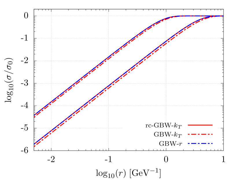
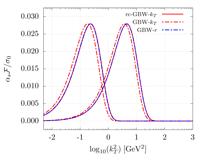
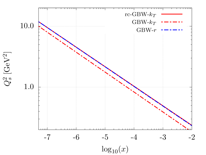
(a) GBW

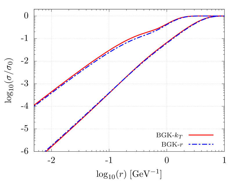
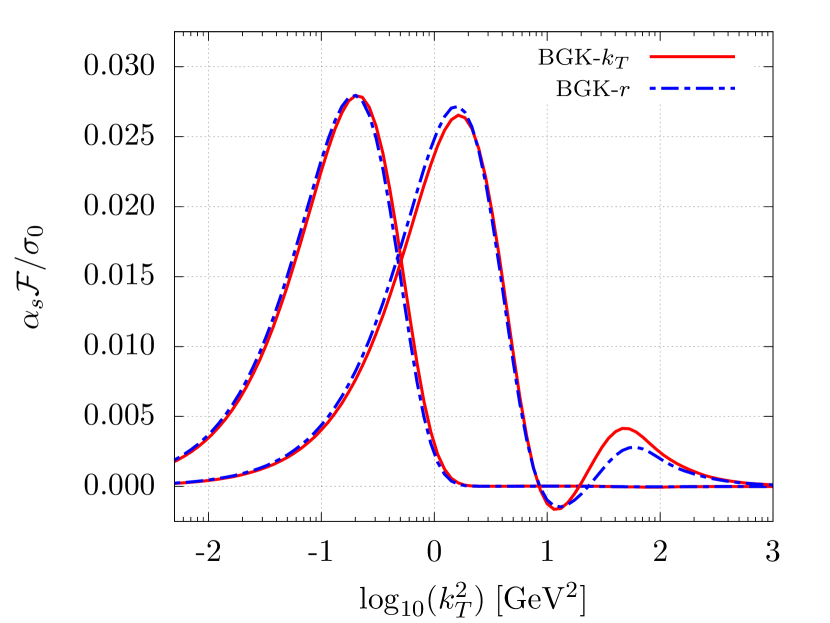
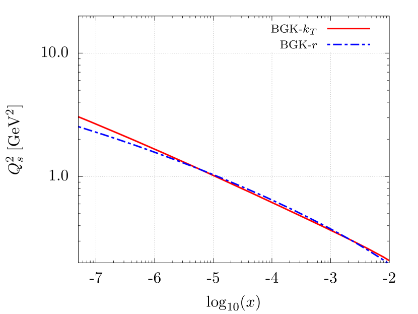
(b) BGK

Figure 2: The dipole cross section, the dipole gluon density at $x=10^{-2},\;10^{-6}$, and the saturation scale for the GBW (left) and the BGK (right) models. Note that the dipole cross section and the gluon density are normalized with $\sigma_{0}^{-1}$.

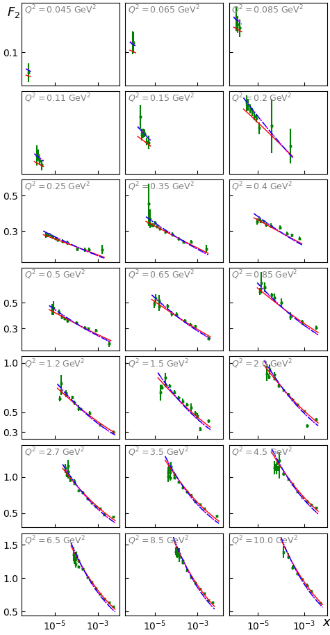
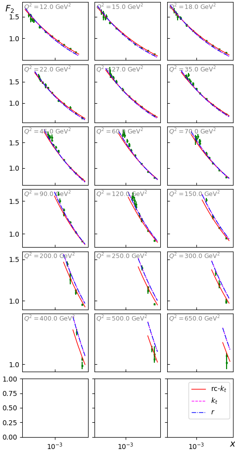
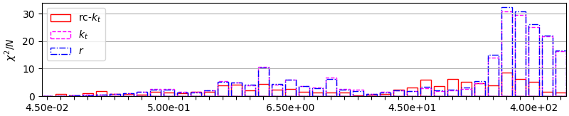
Figure 3: Comparison of $F_{2}$ fro GBW with HERA data. The histogram shows the $\chi^{2}$ value per data point in each frame. Improvement by the running coupling (rc-$k_{T}$) is clearly visible in the high-$Q^{2}$region, while the new fit ($k_{T}$) shows only marginal improvement.

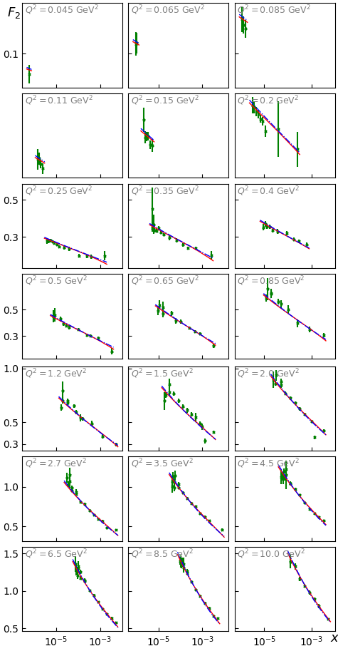
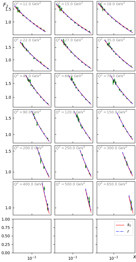
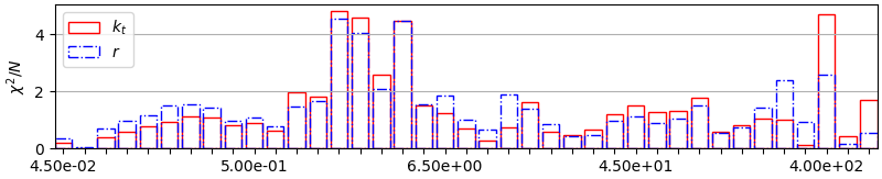
Figure 4: Comparison of $F_{2}$ from BGK with HERA data. The histogram shows the $\chi^{2}$ value per data point in each frame. The overall fit quality remain similar but the quality in each frame changes noticeably. In particularly, the $k_{T}$-formula ($k_{T}$) shows better quality at small $Q^{2}$.

Let us now take a closer look at the parameter $\sigma_{0}$. Recall that the difference between the $k_{T}$-factorization formula and the dipole factorization formula is in $x/z$, and this enters in the GBW formalism as $\tilde{x}$. It is easy to see that, as $x$ grows, the dipole cross section gets suppressed. (Keeping in mind the suppression by the photon wave function in the large-$r$ region.) Such effect was discussed previously in Ref. [58] in the context of the BK equation. In fact, this suppression is the motivation given in Ref. [27] for such modification of $x$, so that, in the small-$Q^{2}$ limit, the total cross section remains finite. Since

$$\left(1+\frac{4m_{f}^{2}}{Q^{2}}\right)\leq\left(1+\frac{k_{T}^{2}}{Q^{2}}+\frac{{\kappa^{\prime}}_{t}^{2}+m_{f}^{2}}{\beta(1-\beta)Q^{2}}\right),$$ (15)

the $k_{T}$-factorization case receives more suppression. Consequently, the normalization factor $\sigma_{0}$ rises to compensate the suppression. Therefore, one can understand the change in $\sigma_{0}$ as a direct consequence of the key difference between the $k_{T}$-factorization and the dipole factorization.

4 Dijet production at EIC

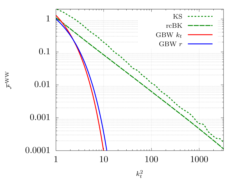
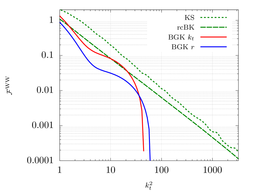
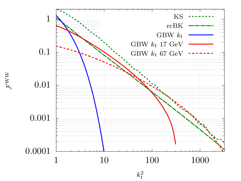
Figure 5: Weizsäcker-Williams gluon density at $x=10^{-3}$. Top row: comparison of the dipole factorization fit and $k_{T}$-factorization fit results. Bottom row: comparison of the respective models with and without the Sudakov factor, at $\mu=17,\;67\ \mathrm{GeV}$.The green dotted line is the KS gluon [41], and the green dashed line is the rcBK gluon [59].

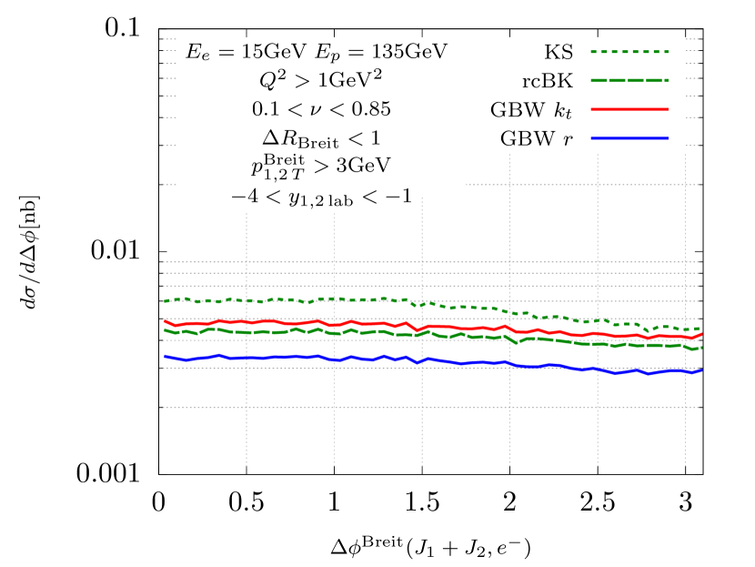
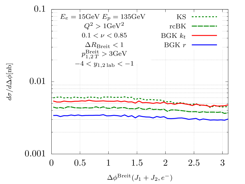
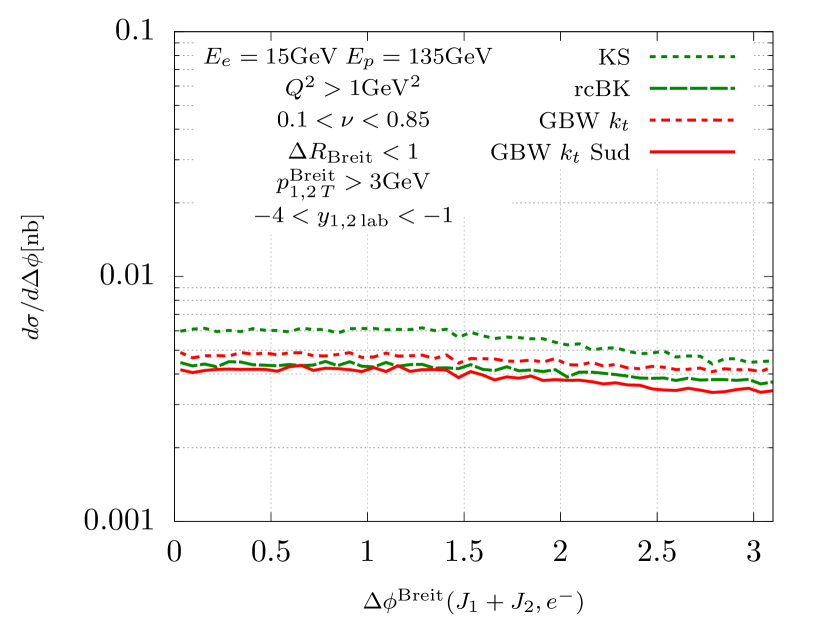
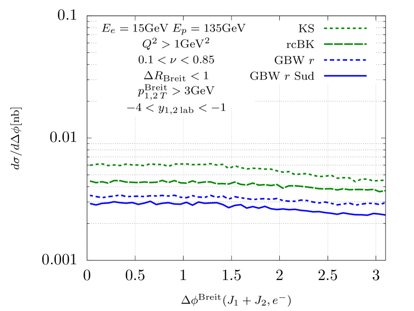
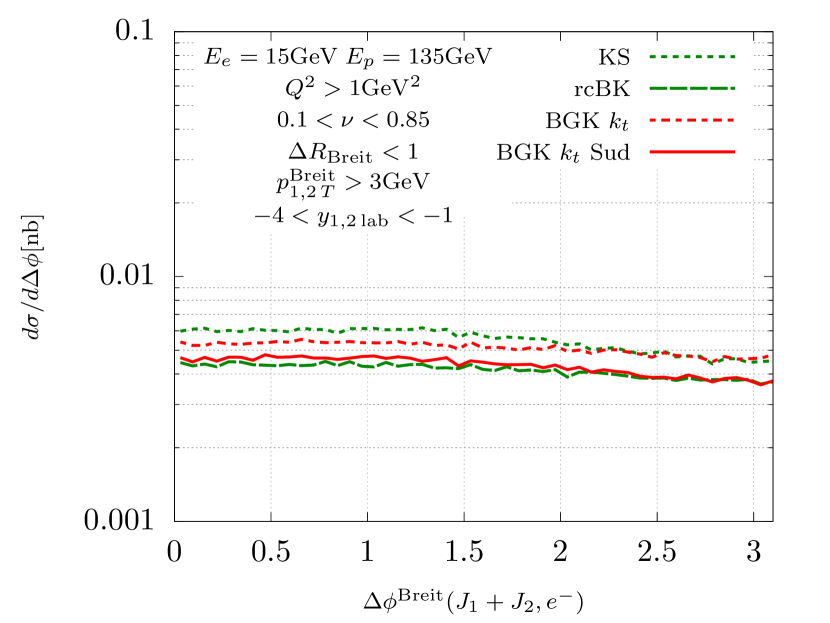
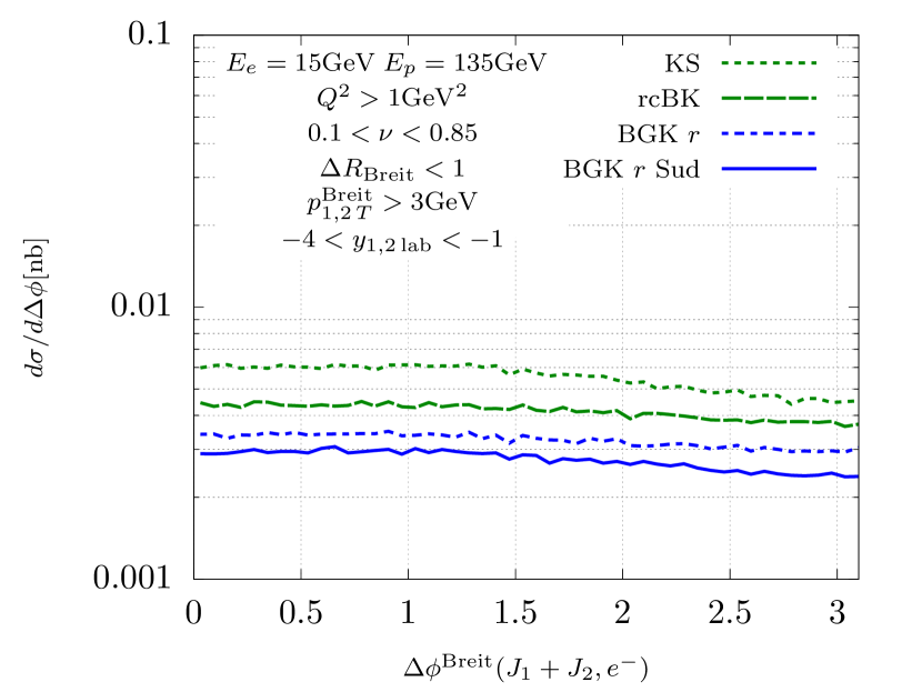
Figure 6: Azimuthal correlation of the jets and the scattered electron in the Breit frame. Top: Comparison of dipole factorization fit and $k_{T}$-factorization fit. Middle & Bottom: Effect of the Sudakov form factor. The green dotted line is the KS gluon [41], and the green dashed line is the rcBK gluon [59].

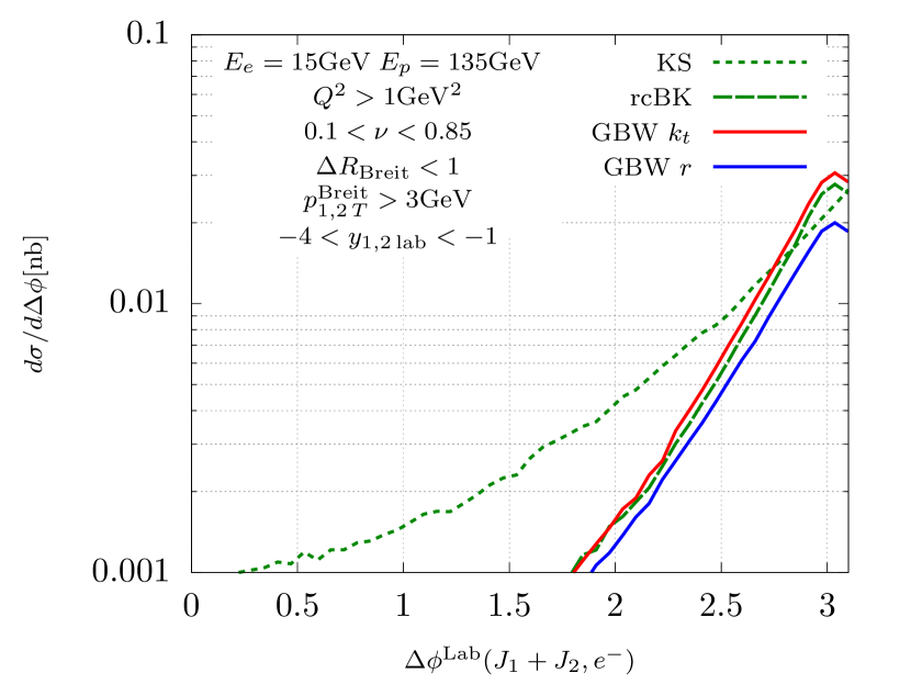
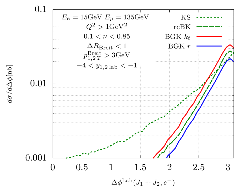
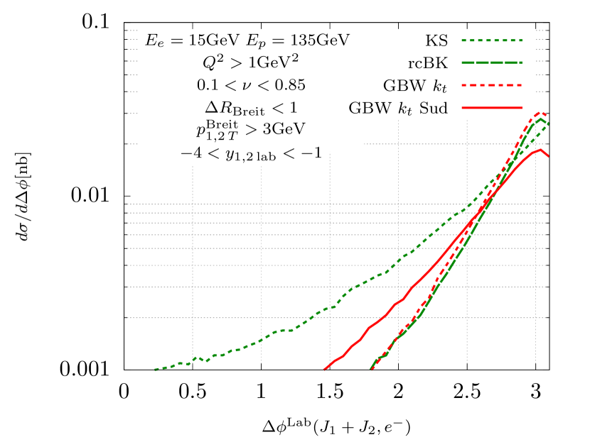
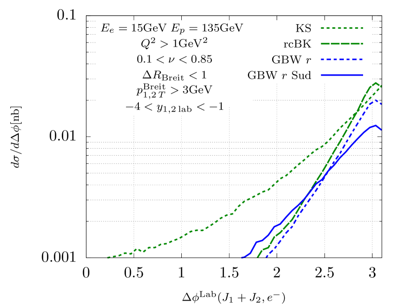
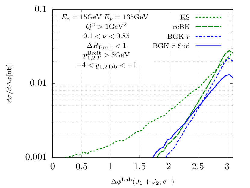
Figure 7: Azimuthal correlation of the jets and the scattered electron in the lab frame. Top: Comparison of dipole factorization fit and $k_{T}$-factorization fit. Middle & Bottom: Effect of the Sudakov form factor. The green dotted line is the KS gluon [41], and the green dashed line is the rcBK gluon [59].

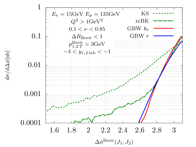
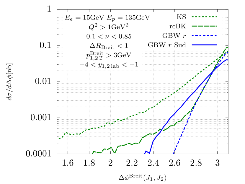
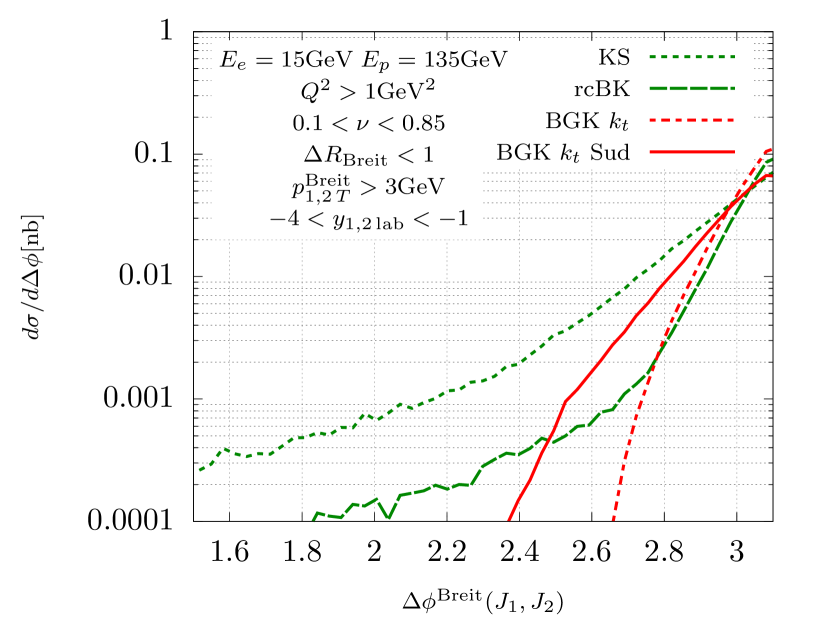
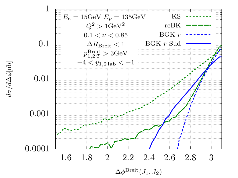
Figure 8: Azimuthal correlation of the jets in the Breit frame. Top: Comparison of dipole factorization fit and $k_{T}$-factorization fit. Middle & Bottom: Effect of the Sudakov form factor. The green dotted line is the KS gluon [41], and the green dashed line is the rcBK gluon [59].

The $F_{2}$ structure function is an inclusive object and it is weakly sensitive to the shape of the gluon density. To probe that shape better, we shall now apply the dipole cross sections obtained in the previous section to the jet correlations at the EIC, following closely the method of Ref. [41].

We consider dijet production in DIS

$$e+p\rightarrow e+J_{1}+J_{2}+X\,.$$ (16)

At the leading order, in the small-$x$ limit, this process is dominated by $q\overline{q}$ jets [13]. It is therefore closely related to the dipole picture we discussed earlier. In the Breit frame, where the photon momentum is given by $q=(0,0,0,Q)$, at the leading order, the jets momentum imbalance $p_{T}\equiv\left|p_{1T}+p_{2T}\right|$ equals the gluon transverse momentum $k_{T}$, where $p_{1T}$ and $p_{2T}$ are transverse momenta of the jets. This makes dijets an interesting process. For the region where $p_{T}\ll P_{T}\sim p_{1T},\,p_{2T}$, one may use power counting to take leading order in $p_{T}/P_{T}$, which leads to the transverse-momentum-dependent (TMD) factorization.

In the large-$N_{c}$ limit of the TMD factorization, there are two types of gluon densities, namely the dipole gluon density and the Weizsäcker-Williams (WW) gluon density [12, 13, 60, 61]. It was shown in Ref. [13], that the dijet process in DIS can directly probe the WW gluon, $\mathcal{F}^{\mathrm{WW}}(x,k^{2})$, where the differential cross section factorizes as

$$\frac{d\sigma^{\gamma^{*}p\rightarrow q\overline{q}X}}{d\mathrm{P.S.}}=\mathcal{F}^{\mathrm{WW}}(x,k_{T}^{2})H_{\gamma^{*}g^{*}\rightarrow q\overline{q}},$$ (17)

with the hard function $H_{\gamma^{*}g^{*}\rightarrow q\overline{q}}$ describing interactions of an off-shell photon with an off-shell gluon producing a $q\overline{q}$ pair. $\mathcal{F}^{\mathrm{WW}}(x,k^{2})$, has an interpretation as a number density of gluons inside a proton, while $\mathcal{F}^{\mathrm{dipole}}(x,k_{T}^{2})$ does not have such an interpretation [12, 13, 61].

We carry out our study in the framework of the Improved Transverse-Momentum-Dependent (ITMD) factorization [62, 60]. This is implemented in the program KaTie [63], which we use to compute the cross sections. The ITMD factorization is a generalization of the TMD factorization, where the momentum imbalance in TMD is restricted to be small [62, 60]. That is to say, ITMD resums $(Q_{s}/k_{T})^{n}$ and $(k_{T}/P_{T})^{n}$ [62, 60], thus extends the region of applicability up to $k_{T}\sim P_{T}$. The difference of Eq. (17) from the regular TMD is that the hard function has an off-shell gluon, $g^{*}$, thus rendering the $k_{T}$ dependence in the hard function as well [62].

Under the Gaussian approximation and assuming $\theta$-like profile of the proton, one can write [60, 61, 12, 13]

$$\mathcal{F}^{\mathrm{WW}}(x,k^{2})=\frac{C_{F}}{2\pi^{3}\alpha_{s}}\int^{\infty}_{0}\frac{dr}{r}J_{0}(rk)\sigma_{\mathrm{dipole\,Adj.}}(x,r),$$ (18)

with the adjoint dipole cross section

$$\sigma_{\mathrm{dipole\,Adj.}}(x,r)=\sigma_{0}\left(1-\left(1-\frac{\sigma_{\mathrm{dipole}}(x,r)}{\sigma_{0}}\right)^{C_{A}/C_{F}}\right).$$ (19)

For the region where the TMD factorization is applicable, $Q_{s}\sim k_{T}\ll P_{T}\sim Q$, one needs to resum the large Sudakov logarithms $\log(k_{T}/Q)$, as well as $\log(1/x)$ [13]. It was shown in Refs. [64, 65, 14] that consistent resummation of such logarithms is possible owing to the separation of corresponding regions (see also Ref. [66]). Resummation of the Sudakov logarithms is achieved by the formula

$$\mathcal{F}^{\mathrm{WW}}(x,k^{2},\mu^{2})=\frac{C_{F}}{2\pi^{3}\alpha_{s}}\int^{\infty}_{0}\frac{dr}{r}J_{0}(rk)e^{-S(r,\mu^{2})}\sigma_{\mathrm{dipole\,Adj.}}(x,r),$$ (20)

where, we use the Sudakov form factor [65, 14],

$$S(r,\mu^{2})=\frac{\alpha_{s}N_{c}}{4\pi}\ln^{2}\left(\frac{\mu^{2}r^{2}}{4e^{-2\gamma_{E}}}\right),$$ (21)

in which $\gamma_{E}$ is the Euler-Mascheroni constant, and we set $\alpha_{s}=0.2$. Following Ref. [41], we study the azimuthal correlations of jets and the final state electron in DIS , where it was argued that this observable is sensitive to the soft emissions and the saturation effects. In this study we focus only on the proton case. The kinematical cuts suggested in Ref. [41] are

$$E_{e} =15\mathrm{GeV} E_{p} =135\mathrm{GeV} Q^{2} >1\mathrm{GeV}^{2}$$

$$0.1< \nu<0.85 \Delta R_{\mathrm{Breit}} <1 p^{\mathrm{Breit}}_{1,2\,T} >3\mathrm{GeV}$$

$$-4< y_{1,2\,\mathrm{lab}}<-1.$$

Grids of the Weizsäcker-Williams gluon density were produced by evaluating Eqs. (19) and (20). The gluon density at $x=10^{-3}$ is plotted in Fig. 5 with the hard-scale-independent Kutak-Sapeta (KS) gluon [67, 41, 68] and the running-coupling BK (rcBK) gluon density [69, 57, 59]. Both of these gluon densities are solutions of evolution equations and treat better perturbative tail at large $k_{T}$. Furthermore, the KS gluon takes into account resummed corrections of higher orders, i.e. kinematical constraint and nonsingular (at low $z$) elements of DGLAP splitting functions [45].

Clearly, as shown in Fig. 5, the GBW and BGK models fall much more quickly than the KS and rcBK gluon densities. In general, expected behaviour in the large-$k_{T}$ region is $\sim k_{T}^{-2}$ [12, 13], while $\sigma_{\mathrm{GBW}}$ behaves like $\sim e^{-k_{T}^{2}}$. As in Ref. [41], the Sudakov factor enhances in the small-$k_{T}$ region and suppresses in the large-$k_{T}$ region. In other words, it broadens the distribution. In comparison to the result of Ref. [41], the effect of broadening by the Sudakov factor is significantly more pronounced in the case of the GBW and BGK models. The hard-scale-dependent GBW and BGK models, as a consequence, become closer to the KS and rcBK gluons, cf. Fig. 2 of Ref. [41].

Figs. 6 and 7 show electron-jets azimuthal correlation in the Breit and in the Lab frame, respectively. In the top row of Fig. 6, we see, for both the GBW and BGK models, better agreements of results with the KS and rcBK for the new $k_{T}$-factorization fits. However the overall normalization of the gluon density depends on the coupling $\alpha_{s}$, which we assumed to be 0.2. Nevertheless, it shows clearly the effect of the parameter $\sigma_{0}$. In the middle and the bottom row, it shows the effects of the Sudakov form factor, which qualitatively agrees with that of Ref. [41], by lowering the cross section.

Fig. 7 shows the electron-jets correlation in the Lab frame. Here, the difference between KS and GBW and BGK is more prominent, while rcBK shows similar pattern to the GBW and BGK models and therefore we can attribute the effects to importance of higher order corrections, as are accounted for in KS gluon. The effects of the Sudakov factor are similar to those in Ref. [41] at relatively high $\Delta\phi$, while at smaller $\Delta\phi$, the effect is reversed (i.e. the cross sections were slightly lowered in Ref. [41], while here, they are significantly increased).

Finally, Fig. 8 shows the jet-jet correlations in the Breit frame. Again, the GBW and BGK models exhibit considerable deviation from the KS gluon. The difference from the previous plot is the disagreement of the GBW/BGK models and the rcBK in the small-$\Delta\phi$ region. Similarly to the previous plots, the Sudakov factor affects the models somewhat differently from the KS gluon in Ref. [41]. The effect enhances the cross section considerably in the small-$\Delta\phi$ region, making it closer to KS gluon result.

The results shown in Figs. 7 and 8 are natural, as back-to-back configuration in the respective observable corresponds to the small-$k_{T}$ region of gluon densities and, as it can be seen clearly in Fig. 5, the GBW and BGK gluons do not fare well in the large-$k_{T}$ region. That is to say that the enhancement in the small-$\Delta\phi$ region is a direct consequence of the broadening by the Sudakov factor.

5 Summary

We have fitted the GBW and BGK saturation models to HERA data [33] using the $k_{T}$-factorization for the structure function $F_{2}$. The main difference between the $k_{T}$- and the dipole factorizations is an argument of the gluon, $x/z$, appearing in the former and being replaced by $x\,(1+4m_{f}^{2}/Q^{2})$ in the latter. In fact, the massive light quarks used in Ref. [27] partially simulate the factor $1/z$, and our fit result indicates such effect, as expected.

We found that the dipole factorization can reproduce the result of the $k_{T}$-factorization formula quite well. The only major difference is in the normalization parameter $\sigma_{0}$, which increases significantly for the $k_{T}$-factorization case. We argued that this change is a direct consequences of the kinematic approximation used in the dipole factorization formula. We have also observed that the explicit inclusion of the running coupling in the GBW model has significant effect on fit quality, particularly in the large-$Q^{2}$ region, where the GBW model performs poorly.

We have applied the new results from our fits for predictions of the dijet process in DIS at EIC. Additionally, effects of the Sudakov form factor were investigated for that process. Results of the electron-jets correlation in the Breit frame agree qualitatively with those of Ref. [41]. Other results, namely the electron-jets in the Lab frame and the jet-jet correlation in the Breit frame, show considerable effects of the Sudakov form factor, which broadens the gluon density.

Appendix A $I_{i}$ in Eq. (7)

The functions $I_{1},\,I_{2},\,I_{3},\,I_{4}$ used in Eq. (7) are defined as [44]

$$\begin{split}\frac{I_{1}}{2\pi}=\frac{N_{1}N_{2}+N_{3}^{2}}{\left(N^{2}_{1}+2N_{1}N_{2}+N_{3}^{2}\right)^{3/2}},&\hskip 28.45274pt\frac{I_{2}}{2\pi}=\frac{N_{3}-(1-2\beta)N_{1}}{(N_{1}+N_{4})\sqrt{N^{2}_{1}+2N_{1}N_{2}+N_{3}^{2}}},\\ \frac{I_{3}}{2\pi}=\frac{N_{1}+N_{2}}{\left(N^{2}_{1}+2N_{1}N_{2}+N_{3}^{2}\right)^{3/2}},&\hskip 28.45274pt\frac{I_{4}}{2\pi}=\frac{2(1-\beta)}{(N_{1}+N_{4})\sqrt{N^{2}_{1}+2N_{1}N_{2}+N_{3}^{2}}},\end{split}$$ (22)

for

$$\begin{split}N_{1}\equiv\beta(1-\beta)Q^{2}+m_{f}^{2},&\hskip 56.9055ptN_{2}\equiv{\kappa^{\prime}}_{t}^{2}+(1-\beta)^{2}k_{T}^{2},\\ N_{3}\equiv{\kappa^{\prime}}_{t}^{2}-(1-\beta)^{2}k_{T}^{2},&\hskip 56.9055ptN_{4}\equiv{\kappa^{\prime}}_{t}^{2}+\beta(1-\beta)k_{T}^{2}.\end{split}$$ (23)

References

- [1] R. G. Roberts. The Structure of the proton: Deep inelastic scattering. Cambridge Monographs on Mathematical Physics. Cambridge University Press, 2 1994.
- [2] John Collins. Foundations of perturbative QCD, volume 32. Cambridge University Press, 11 2013.
- [3] An Assessment of U.S.-Based Electron-Ion Collider Science. The National Academies Press, Washington, DC, 2018.
- [4] Yuri V. Kovchegov and Eugene Levin. Quantum Chromodynamics at High Energy, volume 33. Oxford University Press, 2013.
- [5] S. Catani, M. Ciafaloni, and F. Hautmann. GLUON CONTRIBUTIONS TO SMALL x HEAVY FLAVOR PRODUCTION. Phys. Lett. B, 242:97–102, 1990.
- [6] S. Catani, M. Ciafaloni, and F. Hautmann. High-energy factorization and small x heavy flavor production. Nucl. Phys. B, 366:135–188, 1991.
- [7] John C. Collins and R. Keith Ellis. Heavy quark production in very high-energy hadron collisions. Nucl. Phys. B, 360:3–30, 1991.
- [8] S. Catani, M. Ciafaloni, and F. Hautmann. High-energy factorization in QCD and minimal subtraction scheme. Phys. Lett. B, 307:147–153, 1993.
- [9] S. Catani and F. Hautmann. Quark anomalous dimensions at small x. Phys. Lett. B, 315:157–163, 1993.
- [10] S. Catani and F. Hautmann. High-energy factorization and small x deep inelastic scattering beyond leading order. Nucl. Phys. B, 427:475–524, 1994.
- [11] C. J. Bomhof, P. J. Mulders, and F. Pijlman. The Construction of gauge-links in arbitrary hard processes. Eur. Phys. J. C, 47:147–162, 2006.
- [12] Fabio Dominguez, Bo-Wen Xiao, and Feng Yuan. -factorization for Hard Processes in Nuclei. Phys. Rev. Lett., 106:022301, 2011.
- [13] Fabio Dominguez, Cyrille Marquet, Bo-Wen Xiao, and Feng Yuan. Universality of Unintegrated Gluon Distributions at small x. Phys. Rev. D, 83:105005, 2011.
- [14] Bo-Wen Xiao, Feng Yuan, and Jian Zhou. Transverse Momentum Dependent Parton Distributions at Small-x. Nucl. Phys. B, 921:104–126, 2017.
- [15] I. I. Balitsky and L. N. Lipatov. The Pomeranchuk Singularity in Quantum Chromodynamics. Sov. J. Nucl. Phys., 28:822–829, 1978.
- [16] E. A. Kuraev, L. N. Lipatov, and Victor S. Fadin. The Pomeranchuk Singularity in Nonabelian Gauge Theories. Sov. Phys. JETP, 45:199–204, 1977.
- [17] V. Barone, M. Genovese, Nikolai N. Nikolaev, E. Predazzi, and B. G. Zakharov. Unitarization of structure functions at large 1/x. Phys. Lett. B, 326:161–167, 1994.
- [18] L. V. Gribov, E. M. Levin, and M. G. Ryskin. Semihard Processes in QCD. Phys. Rept., 100:1–150, 1983.
- [19] I. Balitsky. Operator expansion for high-energy scattering. Nucl. Phys. B, 463:99–160, 1996.
- [20] Yuri V. Kovchegov. Small x F(2) structure function of a nucleus including multiple pomeron exchanges. Phys. Rev. D, 60:034008, 1999.
- [21] Alex Kovner and J. Guilherme Milhano. Vector potential versus color charge density in low x evolution. Phys. Rev. D, 61:014012, 2000.
- [22] Alex Kovner, J. Guilherme Milhano, and Heribert Weigert. Relating different approaches to nonlinear QCD evolution at finite gluon density. Phys. Rev. D, 62:114005, 2000.
- [23] Edmond Iancu, Andrei Leonidov, and Larry D. McLerran. Nonlinear gluon evolution in the color glass condensate. 1. Nucl. Phys. A, 692:583–645, 2001.
- [24] Jamal Jalilian-Marian, Alex Kovner, and Heribert Weigert. The Wilson renormalization group for low x physics: Gluon evolution at finite parton density. Phys. Rev. D, 59:014015, 1998.
- [25] Jamal Jalilian-Marian, Alex Kovner, Andrei Leonidov, and Heribert Weigert. The Wilson renormalization group for low x physics: Towards the high density regime. Phys. Rev. D, 59:014014, 1998.
- [26] Jamal Jalilian-Marian, Alex Kovner, Andrei Leonidov, and Heribert Weigert. The BFKL equation from the Wilson renormalization group. Nucl. Phys. B, 504:415–431, 1997.
- [27] Krzysztof J. Golec-Biernat and M. Wusthoff. Saturation effects in deep inelastic scattering at low Q**2 and its implications on diffraction. Phys. Rev. D, 59:014017, 1998.
- [28] J. Bartels, Krzysztof J. Golec-Biernat, and H. Kowalski. A modification of the saturation model: DGLAP evolution. Phys. Rev. D, 66:014001, 2002.
- [29] Henri Kowalski and Derek Teaney. An Impact parameter dipole saturation model. Phys. Rev. D, 68:114005, 2003.
- [30] Larry D. McLerran and Raju Venugopalan. Computing quark and gluon distribution functions for very large nuclei. Phys. Rev. D, 49:2233–2241, 1994.
- [31] Jeffrey R. Forshaw, G. Kerley, and Graham Shaw. Extracting the dipole cross-section from photoproduction and electroproduction total cross-section data. Phys. Rev. D, 60:074012, 1999.
- [32] E. Iancu, K. Itakura, and S. Munier. Saturation and BFKL dynamics in the HERA data at small x. Phys. Lett. B, 590:199–208, 2004.
- [33] I. Abt, A. M. Cooper-Sarkar, B. Foster, V. Myronenko, K. Wichmann, and M. Wing. Investigation into the limits of perturbation theory at low using HERA deep inelastic scattering data. Phys. Rev. D, 96(1):014001, 2017.
- [34] Alfred H. Mueller and Bimal Patel. Single and double BFKL pomeron exchange and a dipole picture of high-energy hard processes. Nucl. Phys. B, 425:471–488, 1994.
- [35] R. Abdul Khalek et al. Science Requirements and Detector Concepts for the Electron-Ion Collider: EIC Yellow Report. Nucl. Phys. A, 1026:122447, 2022.
- [36] Paul Caucal, Farid Salazar, Björn Schenke, Tomasz Stebel, and Raju Venugopalan. Back-to-back inclusive dijets in DIS at small : Gluon Weizsäcker-Williams distribution at NLO. 4 2023.
- [37] Paul Caucal, Farid Salazar, and Raju Venugopalan. Dijet impact factor in DIS at next-to-leading order in the Color Glass Condensate. JHEP, 11:222, 2021.
- [38] Renaud Boussarie, Heikki Mäntysaari, Farid Salazar, and Björn Schenke. The importance of kinematic twists and genuine saturation effects in dijet production at the Electron-Ion Collider. JHEP, 09:178, 2021.
- [39] Pieter Taels, Tolga Altinoluk, Guillaume Beuf, and Cyrille Marquet. Dijet photoproduction at low x at next-to-leading order and its back-to-back limit. JHEP, 10:184, 2022.
- [40] Tolga Altinoluk, Renaud Boussarie, Cyrille Marquet, and Pieter Taels. TMD factorization for dijets + photon production from the dilute-dense CGC framework. JHEP, 07:079, 2019.
- [41] Andreas van Hameren, Piotr Kotko, Krzysztof Kutak, Sebastian Sapeta, and Elżbieta Żarów. Probing gluon number density with electron-dijet correlations at EIC. Eur. Phys. J. C, 81(8):741, 2021.
- [42] Krzysztof J. Golec-Biernat and M. Wusthoff. Saturation in diffractive deep inelastic scattering. Phys. Rev. D, 60:114023, 1999.
- [43] A. Bialas, H. Navelet, and Robert B. Peschanski. QCD dipole model and K(t) factorization. Nucl. Phys. B, 593:438–450, 2001.
- [44] M. Kimber. Unintegrated parton distributions. PhD thesis, Durham U., 2001.
- [45] J. Kwiecinski, Alan D. Martin, and A. M. Stasto. A Unified BFKL and GLAP description of F2 data. Phys. Rev. D, 56:3991–4006, 1997.
- [46] Nikolai N. Nikolaev and B. G. Zakharov. Color transparency and scaling properties of nuclear shadowing in deep inelastic scattering. Z. Phys. C, 49:607–618, 1991.
- [47] Agnieszka Łuszczak, Marta Łuszczak, and Wolfgang Schäfer. Unintegrated gluon distributions from the color dipole cross section in the BGK saturation model. Phys. Lett. B, 835:137582, 2022.
- [48] G. Beuf, H. Hänninen, T. Lappi, and H. Mäntysaari. Color Glass Condensate at next-to-leading order meets HERA data. Phys. Rev. D, 102:074028, 2020.
- [49] K. S. Kolbig. PROGRAMS FOR COMPUTING THE LOGARITHM OF THE GAMMA FUNCTION AND THE DIGAMMA FUNCTION FOR COMPLEX ARGUMENT. 4 1972.
- [50] M. Galassi, J. Davies, J. Theiler, B. Gough, and G. Jungman. GNU Scientific Library - Reference Manual, Third Edition, for GSL Version 1.12 (3. ed.). 2009.
- [51] T. Hahn. CUBA: A Library for multidimensional numerical integration. Comput. Phys. Commun., 168:78–95, 2005.
- [52] R. Brun and F. Rademakers. ROOT: An object oriented data analysis framework. Nucl. Instrum. Meth. A, 389:81–86, 1997.
- [53] Fred James and Matthias Winkler. MINUIT User’s Guide. 6 2004.
- [54] Tomoki Goda, Krzysztof Kutak, and Sebastian Sapeta. Sudakov effects and the dipole amplitude. Nucl. Phys. B, 990:116155, 2023.
- [55] J. L. Albacete, N. Armesto, J. G. Milhano, C. A. Salgado, and U. A. Wiedemann. Numerical analysis of the Balitsky-Kovchegov equation with running coupling: Dependence of the saturation scale on nuclear size and rapidity. Phys. Rev. D, 71:014003, 2005.
- [56] Javier L. Albacete and Yuri V. Kovchegov. Solving high energy evolution equation including running coupling corrections. Phys. Rev. D, 75:125021, 2007.
- [57] Javier L. Albacete, Nestor Armesto, Jose Guilherme Milhano, Paloma Quiroga-Arias, and Carlos A. Salgado. AAMQS: A non-linear QCD analysis of new HERA data at small-x including heavy quarks. Eur. Phys. J. C, 71:1705, 2011.
- [58] K. Kutak and A. M. Stasto. Unintegrated gluon distribution from modified BK equation. Eur. Phys. J. C, 41:343–351, 2005.
- [59] Martin Hentschinski, Krzysztof Kutak, and Robert Straka. Maximally entangled proton and charged hadron multiplicity in Deep Inelastic Scattering. Eur. Phys. J. C, 82(12):1147, 2022.
- [60] A. van Hameren, P. Kotko, K. Kutak, C. Marquet, E. Petreska, and S. Sapeta. Forward di-jet production in p+Pb collisions in the small-x improved TMD factorization framework. JHEP, 12:034, 2016. [Erratum: JHEP 02, 158 (2019)].
- [61] Bo-Wen Xiao. Low- Physics in Collisions and at the EIC. Nucl. Phys. A, 967:257–264, 2017.
- [62] P. Kotko, K. Kutak, C. Marquet, E. Petreska, S. Sapeta, and A. van Hameren. Improved TMD factorization for forward dijet production in dilute-dense hadronic collisions. JHEP, 09:106, 2015.
- [63] A. van Hameren. KaTie : For parton-level event generation with -dependent initial states. Comput. Phys. Commun., 224:371–380, 2018.
- [64] A. H. Mueller, Bo-Wen Xiao, and Feng Yuan. Sudakov Resummation in Small- Saturation Formalism. Phys. Rev. Lett., 110(8):082301, 2013.
- [65] A. H. Mueller, Bo-Wen Xiao, and Feng Yuan. Sudakov double logarithms resummation in hard processes in the small-x saturation formalism. Phys. Rev. D, 88(11):114010, 2013.
- [66] Maxim Nefedov. Sudakov resummation from the BFKL evolution. Phys. Rev. D, 104(5):054039, 2021.
- [67] Krzysztof Kutak and Sebastian Sapeta. Gluon saturation in dijet production in p-Pb collisions at Large Hadron Collider. Phys. Rev. D, 86:094043, 2012.
- [68] N. A. Abdulov et al. TMDlib2 and TMDplotter: a platform for 3D hadron structure studies. Eur. Phys. J. C, 81(8):752, 2021.
- [69] Ian Balitsky. Quark contribution to the small-x evolution of color dipole. Phys. Rev. D, 75:014001, 2007.